跳到论文正文
W Papers独立论文阅读器 arXiv:1805.11710 论文正文 计算阅读时间 · 0%
引用这篇论文根据当前论文元数据生成,正式投稿前建议核对。


License: arXiv.org perpetual non-exclusive license
arXiv:1805.11710v1 [cs.LG] 29 May 2018

Active and Adaptive Sequential learning

Yuheng Bu ††thanks: Equal contribution††thanks: ECE Department and the Coordinated Science Laboratory, University of Illinois at Urbana-Champaign, Urbana, IL, USA. Email: {bu3, vvv}@illinois.edu    Jiaxun Lu 11footnotemark: 1 ††thanks: EE Department, Tsinghua University, Beijing, China. Email: lujx14@mails.tsinghua.edu.cn    Venugopal V. Veeravalli 22footnotemark: 2
Abstract

A framework is introduced for actively and adaptively solving a sequence of machine learning problems, which are changing in bounded manner from one time step to the next. An algorithm is developed that actively queries the labels of the most informative samples from an unlabeled data pool, and that adapts to the change by utilizing the information acquired in the previous steps. Our analysis shows that the proposed active learning algorithm based on stochastic gradient descent achieves a near-optimal excess risk performance for maximum likelihood estimation. Furthermore, an estimator of the change in the learning problems using the active learning samples is constructed, which provides an adaptive sample size selection rule that guarantees the excess risk is bounded for sufficiently large number of time steps. Experiments with synthetic and real data are presented to validate our algorithm and theoretical results.


1 Introduction

Machine learning problems that vary in a bounded manner over time naturally arise in many applications. For example, in personalized recommendation systems [9, 15], the preferences of users might change with fashion trends. Since acquiring new training samples from users can be expensive in practice, a recommendation system needs to update the machine learning model and adapt to this change using as few new samples as possible.

In such problems, we are given a large set of unlabeled samples, and the learning tasks are solved by minimizing the expected value of an appropriate loss function on this unlabeled data pool at each time tt. To capture the idea that the sequence of learning problems is changing in a bounded manner, we assume the following bound holds

‖θt∗−θt−1∗‖2≤ρ,∀t≥2,\|\theta_{t}^{*}-\theta_{t-1}^{*}\|_{2}\leq\rho,\quad\forall t\geq 2, (1)

where θt∗\theta_{t}^{*} is the true minimizer of the loss functions at time tt, and ρ\rho is a finite upper bound on the change of minimizers, which needs to be estimated in practice.

To tackle this sequential learning problem, we propose an active and adaptive algorithm to learn the approximate minimizers θ^t\hat{\theta}_{t} of the loss function. At each time tt, our algorithm actively queries the labels of KtK_{t} samples from the unlabeled data pool, with a well-designed active sampling distribution, which is adaptive to the change in the minimizers by utilizing the information acquired in the previous steps. In particular, we adaptively select KtK_{t} and construct θ^t\hat{\theta}_{t} such that the excess risk [13] is bounded at each time tt.

The challenges of this active and adaptive sequential learning problem arise in three aspects: 1) we need to determine which samples are more informative for solving the task at the current time step based on the information acquired in the previous time steps to conduct active learning; 2) to achieve a desired bounded excess risk with as few new samples as possible, we need to understand the tradeoff between the solution accuracy and the adaptively determined sample complexity KtK_{t}; 3) the change in the minimizers ρ\rho is unknown and we need to estimate it.

Our contributions in this paper can be summarized as follows. We propose an active and adaptive learning framework with theoretical guarantees to solve a sequence of learning problems, which ensures a bounded excess risk for each individual learning task when tt is sufficiently large. We construct a new estimator of the change in the minimizers ρ^t\hat{\rho}_{t} with active learning samples and show that this estimate upper bounds the true parameter ρ\rho almost surely. We test our approaches on a synthetic regression problem, and further apply it to a recommendation system that tracks changes in preferences of customers. Our experiments demonstrate that our algorithm achieves a better performance compared to the other baseline algorithms in these scenarios.

1.1 Related Work

Our active and adaptive learning problem has relations with multi-task learning (MTL) and transfer learning. In multi-task learning, the goal is to learn several tasks simultaneously as in [2, 10, 21] by exploiting the similarities between the tasks. In transfer learning, prior knowledge from one source task is transferred to another target task either with or without additional training data [14]. Multi-task learning could be applied to solve our problem by running a MTL algorithm at each time, while remembering all prior tasks. However, this approach incurs a heavy memory and computational burden. Transfer learning lacks the sequential nature of our problem, and there is no active learning component in both works. For multi-task and transfer learning, there are theoretical guarantees on regret for some algorithms [1], while we provide an excess risk guarantee for each individual task.

In concept drift problem, stream of incoming data that changes over time is observed, and we try to predict some properties of each piece of data as it arrives. After prediction, a loss is revealed as the feedback in [17]. Some approaches for concept drift use iterative algorithms such as stochastic gradient descent, but without specific models on how the data changes, there is no theoretical guarantees for these algorithms.

Our work is of course related to active learning [8, 4], in which a learning algorithm is able to interactively query the labels of samples from an unlabeled data pool to achieve better performance. A standard approach to active learning is to select the unlabeled samples by optimizing specific statistics of these samples [7]. For example, with the goal of minimizing the expected excess risk in maximum likelihood estimation, the authors of [6, 16] propose a two-stage algorithm based on Fisher information ratio to select the most informative samples, and show that it is optimal in terms of the convergence rate. We apply similar algorithms in our problem, but the first stage of estimating the Fisher information using labeled samples to conduct active learning can be skipped by exploiting the bounded nature of the change, and utilizing information obtained in previous time steps.

Our approach is closely related to prior work on adaptive sequential learning [20, 19], where the training samples are drawn passively and the adaptation is only in the selection of the number of training samples KtK_{t} at each time step.

The rest of the paper is organized as follows. In Section 2, we describe the problem setting considered. In Section 3, we present our active and adaptive learning algorithm. In Section 4, we provide the theoretical analysis which motivates the proposed algorithm. In Section 5, we test our algorithm on synthetic and real data. Finally, in Section 6, we provide some concluding remarks.

2 Problem Setting

Throughout this paper, we use lower case letters to denote scalars and vectors, and use upper case letters to denote random variables and matrices. All logarithms are the natural ones. We use II to denote an identity matrix of appropriate size. We use the superscript (⋅)⊤(\cdot)^{\top} to denote the transpose of a vector or a matrix, and use Tr⁡(A)\mathrm{Tr}(A) to denote the trace of a square matrix AA. We denote ‖x‖A=x⊤​A​x\|x\|_{A}=\sqrt{x^{\top}Ax} for a vector xx and a matrix AA of appropriate dimensions.

We consider the active and adaptive sequential learning problem in the maximum likelihood estimation (MLE) setting. At each time tt, we are given a pool 𝒮t={x1,t,⋯,xN,t}\mathcal{S}_{t}=\{x_{1,t},\cdots,x_{N,t}\} of NtN_{t} unlabeled samples drawn from some instance space 𝒳\mathcal{X}. We have the ability to interactively query the labels of KtK_{t} of these samples from a label space 𝒴\mathcal{Y}. In addition, we are given a parameterized family of distribution models ℳ={p⁡(y|x,θt),θt∈Θ}\mathcal{M}=\{p(y|x,\theta_{t}),\theta_{t}\in\Theta\}, where Θ⊆ℝd\Theta\subseteq\mathbb{R}^{d}. We assume that there exists an unknown parameter θt∗∈Θ\theta_{t}^{*}\in\Theta such that the label yty_{t} of xt∈𝒮tx_{t}\in\mathcal{S}_{t} is actually generated from the distribution p⁡(yt|xt,θt∗)p(y_{t}|x_{t},\theta_{t}^{*}).

For any x∈𝒳x\in\mathcal{X}, y∈𝒴y\in\mathcal{Y} and θ∈Θ\theta\in\Theta, we let the loss function be the negative log-likelihood with parameter θ\theta, i.e.,

ℓ⁡(y|x,θ)≜−log⁡p⁡(y|x,θ),p⁡(y|x,θ)∈ℳ.\ell(y|x,\theta)\triangleq-\log p(y|x,\theta),\quad p(y|x,\theta)\in\mathcal{M}. (2)

Then, the expected loss function over the uniform distribution on the data pool 𝒮t\mathcal{S}_{t} can be written as

LUt​(θ)≜𝔼X∼Ut,Y∼p⁡(Y|X,θt∗)​[ℓ⁡(Y|X,θ)],L_{U_{t}}(\theta)\triangleq\mathbb{E}_{X\sim U_{t},Y\sim p(Y|X,\theta_{t}^{*})}[\ell(Y|X,\theta)], (3)

where we use UtU_{t} to denote the uniform distribution over the samples in 𝒮t\mathcal{S}_{t}. It can be seen that the minimizer of LUt​(θ)L_{U_{t}}(\theta) is the true parameter θt∗\theta_{t}^{*}. As mentioned in (1), we assume that θt∗\theta_{t}^{*} is changing at a bounded but unknown rate, i.e., ‖θt∗−θt−1∗‖2≤ρ\|\theta_{t}^{*}-\theta_{t-1}^{*}\|_{2}\leq\rho, for t≥2t\geq 2.

The quality of our approximate minimizers θ^t\hat{\theta}_{t} are evaluated through a mean tracking criterion, which means that the excess risk of θ^t\hat{\theta}_{t} is bounded at each time step tt, i.e.,

𝔼⁡[LUt​(θ^t)−LUt​(θt∗)]≤ε.\mathbb{E}[L_{U_{t}}(\hat{\theta}_{t})-L_{U_{t}}({\theta}_{t}^{*})]\leq\varepsilon. (4)

Thus, our goal is to actively and adaptively select the smallest number of samples KtK_{t} in 𝒮t\mathcal{S}_{t} to query labels, and sequentially construct an estimate of θ^t\hat{\theta}_{t} satisfying the above mean tracking criterion for each time step tt. Note that it is allowed to query the label of the same sample multiple times.

Let Γt\Gamma_{t} be an arbitrary sampling distribution on 𝒮t\mathcal{S}_{t}. Then, the following MLE using Γt\Gamma_{t}

θ^Γt≜argminθ∈Θ1Kt​∑k=1Ktℓ⁡(Yk,t|Xk,t,θ),\hat{\theta}_{\Gamma_{t}}\triangleq\argmin_{\theta\in\Theta}\frac{1}{K_{t}}\sum_{k=1}^{K_{t}}\ell(Y_{k,t}|X_{k,t},\theta), (5)

can be viewed as an empirical risk minimizer (ERM) of (3), where Xk,t∼ΓtX_{k,t}\sim\Gamma_{t}, Yk,t∼p⁡(Y|Xk,t,θt∗)Y_{k,t}\sim p(Y|X_{k,t},\theta_{t}^{*}).

To ensure that our algorithm works correctly, we require the following assumption on the Hessian matrix of ℓ⁡(y|x,θ)\ell(y|x,\theta), which determines the Fisher information matrix.

Assumption 1.

For any x∈𝒳x\in\mathcal{X}, y∈𝒴y\in\mathcal{Y}, θ∈Θ\theta\in\Theta, H⁡(x,θ)≜∂2ℓ⁡(y|x,θ)∂θ2H(x,\theta)\triangleq\frac{\partial^{2}\ell(y|x,\theta)}{\partial\theta^{2}} is a function of only xx and θ\theta and does not depend on yy.

Assumption 1 holds for many practical models, such as generalized linear model, logistic regression and conditional random fields [6]. Moreover, for θ∈Θ\theta\in\Theta, we denote IΓt​(θ)≜𝔼X∼Γt​[H⁡(X,θ)]I_{\Gamma_{t}}(\theta)\triangleq\mathbb{E}_{X\sim\Gamma_{t}}[H(X,\theta)] as the Fisher information matrix under sampling distribution Γt\Gamma_{t}.

3 Algorithm

The main idea of our algorithm is to adaptively choose the number of samples KtK_{t} based on the estimated change in the minimizers ρ^t−1\hat{\rho}_{t-1} such that the mean tracking criterion in (4) is satisfied, then actively query the labels of these KtK_{t} samples with a well-designed sampling distribution Γt\Gamma_{t}, and finally perform MLE in (5) using a stochastic gradient descent (SGD) algorithm over the labeled samples. By executing this algorithm iteratively, we can sequentially learn θ^t\hat{\theta}_{t} over all the considered time steps. The algorithm is formally presented in Algorithm 1.

To ensure a good performance with limited querying samples, it is essential to construct Γt\Gamma_{t} carefully. Motivated by Lemma 1 in Section 4.2, the convergence rate of the excess risk for ERM using KtK_{t} samples from Γt\Gamma_{t} is Tr⁡(IΓt−1​(θt∗)​IUt​(θt∗))/Kt\mathrm{Tr}(I_{\Gamma_{t}}^{-1}(\theta_{t}^{*})I_{U_{t}}(\theta_{t}^{*}))/K_{t}. Thus, the optimal sampling distribution Γt∗\Gamma_{t}^{*} should be the one that minimizes Tr⁡(IΓt−1​(θt∗)​IUt​(θt∗))\mathrm{Tr}(I_{\Gamma_{t}}^{-1}(\theta_{t}^{*})I_{U_{t}}(\theta_{t}^{*})), which relies on the unknown parameter θt∗\theta_{t}^{*}. Based on the bounded nature of the change in (1), we solve this problem by approximating θt∗\theta_{t}^{*} with θ^t−1\hat{\theta}_{t-1} and generate the sampling distribution Γ^t∗\hat{\Gamma}_{t}^{*} by minimizing Tr⁡(IΓt−1​(θ^t−1)​IUt​(θ^t−1))\mathrm{Tr}(I_{\Gamma_{t}}^{-1}(\hat{\theta}_{t-1})I_{U_{t}}(\hat{\theta}_{t-1})) (Step 1).

Algorithm 1 Active and Adaptive Sequential Learning
 Input: Sample pool 𝒮t={x1,t,⋯,xN,t}\mathcal{S}_{t}=\{x_{1,t},\cdots,x_{N,t}\}, the previous estimation θ^t−1\hat{\theta}_{t-1}, ρ^t−1\hat{\rho}_{t-1} and the desired mean tracking accuracy ε\varepsilon.
 1: Solve the following semidefinite programming problem (see Section 4.2)
Γ^t∗=argminΓt∈ℝNtTr​[IΓt−1​(θ^t−1)​IUt​(θ^t−1)]s.t.\displaystyle\hat{\Gamma}_{t}^{*}=\argmin_{\Gamma_{t}\in\mathbb{R}^{N_{t}}}\,\,\,{\mathrm{Tr}}[I_{\Gamma_{t}}^{-1}(\hat{\theta}_{t-1})I_{U_{t}}(\hat{\theta}_{t-1})]\quad\textrm{s.t.}\,\,\, {IΓt​(θ^t−1)=∑i=1NtΓi,t​H​(xi,t,θ^t−1),∑i=1NtΓi,t=1,Γi,t∈[0,1].\displaystyle\begin{cases}I_{\Gamma_{t}}(\hat{\theta}_{t-1})=\sum_{i=1}^{N_{t}}\Gamma_{i,t}H(x_{i,t},\hat{\theta}_{t-1}),\\ \sum_{i=1}^{N_{t}}\Gamma_{i,t}=1,\,\Gamma_{i,t}\in[0,1].\end{cases}
 2: Choose Kt∗K_{t}^{*} based on ρ^t−1\hat{\rho}_{t-1} such that it is the minimum number of samples required to meet the mean tracking criterion (see Section 4.3).
 3: Generate Kt∗K^{*}_{t} samples using the distribution Γ¯t=αt​Γ^t∗+(1−αt)​Ut\bar{\Gamma}_{t}=\alpha_{t}\hat{\Gamma}_{t}^{*}+(1-\alpha_{t})U_{t} on unlabeled data pool 𝒮t\mathcal{S}_{t}, where αt∈(0,1)\alpha_{t}\in(0,1). Query their labels and get the labeled set 𝒮t′={(xk,t,yk,t)}k=1Kt∗\mathcal{S}_{t}^{\prime}=\{(x_{k,t},y_{k,t})\}_{k=1}^{K_{t}^{*}}.
 4: Solve the MLE using labeled set St′S_{t}^{\prime} with a SGD algorithm initialized at θ^t−1\hat{\theta}_{t-1},
θ^t=argminθt∈Θ∑(xk,t,yk,t)∈𝒮t′ℓ(yk,t|xk,t,θt).\hat{\theta}_{t}=\argmin_{\theta_{t}\in\Theta}\sum_{(x_{k,t},y_{k,t})\in\mathcal{S}_{t}^{\prime}}\ell(y_{k,t}|x_{k,t},\theta_{t}).
 5: Update the estimate of ρ^t\hat{\rho}_{t} using estimator defined in Section 4.4 for ∀t≥2\forall t\geq 2.
 Output: θ^t\hat{\theta}_{t}, ρ^t\hat{\rho}_{t}.

Then, as shown in Section 4.3, we use the minimum number of samples Kt∗K_{t}^{*} such that the mean tracking criterion is satisfied, and actively draw samples from Γ¯t\bar{\Gamma}_{t} to estimate θ^t\hat{\theta}_{t} (Steps 2-4). Note that the distribution Γ^t∗\hat{\Gamma}_{t}^{*} is modified slightly to Γ¯t\bar{\Gamma}_{t} in Step 3 to ensure it still has the full support of 𝒮t\mathcal{S}_{t}.

Finally, based on the current and previous estimation θ^t\hat{\theta}_{t} and θ^t−1\hat{\theta}_{t-1}, we update the estimate of the bounded change rate ρ^t\hat{\rho}_{t} by the estimator proposed in Section 4.4.

It is easy to see that the active nature of Algorithm 1 comes from the active sampling distribution, which is constructed by minimizing the Fisher information ratio as in Step 1. But the adaptivity of Algorithm 1 is more complex and results from the following three aspects: 1) The sampling distribution is adaptive to the bounded change through the replacement of θt∗\theta^{*}_{t} with θ^t−1\hat{\theta}_{t-1} in Step 1; 2) The sample size selection rule is adaptive through the selection of the minimum number of samples required in Step 2; 3) The SGD is adaptive through the initialization by θ^t−1\hat{\theta}_{t-1} in Step 4.

4 Theoretical Performance Guarantees

In this section, we present the theoretical analysis of Algorithm 1. We first introduce the assumptions needed. Then, in Section 4.2, we provide the analysis of the active sampling distribution. In Section 4.3, we present theoretical guarantees on the sample size selection rules which meet the mean tracking criterion in (4). In Section 4.4, we describe the proposed estimator ρ^t\hat{\rho}_{t}. The proofs of the theorems and all the supporting lemmas will be presented in the Appendices.

4.1 Assumptions

For the purpose of analysis, the following regularity assumption on the log-likelihood function ℓ\ell is required to establish the standard Local Asymptotic Normality of the MLE [18].

Assumption 2 (Regularity conditions).
  1. 1.

    Regularity conditions for MLE:

    1. (a)

      Compactness: Θ\Theta is compact and θt∗\theta_{t}^{*} is an interior point of Θ\Theta for each tt.

    2. (b)

      Smoothness: ℓ⁡(y|x,θ)\ell(y|x,\theta) is smooth in the following sense: the first, second and third derivatives of θ\theta exist at all interior points of Θ\Theta.

    3. (c)

      Strong Convexity: For each tt and θ∈Θ\theta\in\Theta, IUt​(θ)⪰m​II_{U_{t}}(\theta)\succeq mI with m>0m>0, and hence IUt​(θ)I_{U_{t}}(\theta) is positive definite and invertible.

    4. (d)

      Boundedness: For all θ∈Θ\theta\in\Theta, the largest eigenvalue of IUt​(θ)I_{U_{t}}(\theta) is upper bounded by LbL_{b}.

  2. 2.

    Concentration at θt∗\theta_{t}^{*}: For all tt, and any xt∈𝒮tx_{t}\in\mathcal{S}_{t}, yt∈𝒴y_{t}\in\mathcal{Y},

    ∥∇ℓ(yt|xt,θt∗)∥IUt​(θt∗)−1≤L1and∥IUt(θt∗)−1/2H(x,θt∗)IUt(θt∗)−1/2∥≤L2\displaystyle\Big\|\nabla\ell(y_{t}|x_{t},\theta_{t}^{*})\Big\|_{I_{U_{t}}(\theta_{t}^{*})^{-1}}\leq L_{1}\quad\mbox{and}\quad\Big\|I_{U_{t}}(\theta_{t}^{*})^{-1/2}H(x,\theta_{t}^{*})I_{U_{t}}(\theta_{t}^{*})^{-1/2}\Big\|\leq L_{2} (6)

    holds with probability one.

  3. 3.

    Lipschitz continuity: For all tt, there exists a neighborhood BtB_{t} of θt∗\theta_{t}^{*} and a constant L3L_{3}, such that for all xt∈𝒮tx_{t}\in\mathcal{S}_{t}, H⁡(xt,θ)H(x_{t},\theta) are L3L_{3}-Lipschitz in this neighborhood, namely,

    ∥IUt(θt∗)−1/2(H(xt,θ)−H(xt,θ′))IUt(θt∗)−1/2∥≤L3∥θ−θ′∥IUt​(θt∗)\displaystyle\Big\|I_{U_{t}}(\theta_{t}^{*})^{-1/2}\big(H(x_{t},\theta)-H(x_{t},\theta^{\prime})\big)I_{U_{t}}(\theta_{t}^{*})^{-1/2}\Big\|\leq L_{3}\|\theta-\theta^{\prime}\|_{I_{U_{t}}(\theta_{t}^{*})} (7)

    holds for θ,θ′∈Bt\theta,\theta^{\prime}\in B_{t}.

In addition, we need the following assumption to prove that replacing θt∗\theta_{t}^{*} with θ^t−1\hat{\theta}_{t-1} in Algorithm 1 does not change the performance of the active learning algorithm in terms of the convergence rate. This assumption is satisfied by many classes of models, including the generalized linear model [6].

Assumption 3 (Point-wise self-concordance).

For all tt, there exists a constant L4L_{4}, such that

−L4​‖θt−θt∗‖2​H​(x,θt∗)⪯H⁡(x,θt)−H⁡(x,θt∗)⪯L4​‖θt−θt∗‖2​H​(x,θt∗).\displaystyle-L_{4}\|\theta_{t}-\theta_{t}^{*}\|_{2}H(x,\theta_{t}^{*})\preceq H(x,\theta_{t})-H(x,\theta_{t}^{*})\preceq L_{4}\|\theta_{t}-\theta_{t}^{*}\|_{2}H(x,\theta_{t}^{*}). (8)

4.2 Optimal Active Learning Sampling Distribution

In this subsection, we provide the intuition and analysis of Step 1 in Algorithm 1. The construction of the active sampling distribution Γt\Gamma_{t} is motivated by the following lemma, which characterizes the convergence rate of the ERM solution θ^Γt\hat{\theta}_{\Gamma_{t}} defined in (5) when ρ\rho and θt−1∗\theta_{t-1}^{*} are known.

Lemma 1.

Suppose Assumptions 1 and 2 hold, and let Θt≜{θt|‖θt−θt−1∗‖≤ρ}\Theta_{t}\triangleq\{\theta_{t}|\|\theta_{t}-\theta_{t-1}^{*}\|\leq\rho\}. For any sampling distribution Γt\Gamma_{t} on 𝒮t\mathcal{S}_{t}, suppose that IΓt​(θt∗)⪰C​IUt​(θt∗)I_{\Gamma_{t}}(\theta_{t}^{*})\succeq CI_{U_{t}}(\theta_{t}^{*}) holds for some constant C<1C<1. Then, for sufficiently large KtK_{t}, such that γt≜𝒪⁡(1C2​(L1​L3+L2)​log⁡d​KtKt)<1\gamma_{t}\triangleq\mathcal{O}\big(\frac{1}{C^{2}}(L_{1}L_{3}+\sqrt{L_{2}})\sqrt{\frac{\log dK_{t}}{K_{t}}}\big)<1, the excess risk of θ^Γt\hat{\theta}_{\Gamma_{t}} can be bounded as

(1−γt)​τt2Kt−L12C​Kt2≤𝔼⁡[LUt​(θ^Γt)−LUt​(θt∗)]≤(1+γt)​τt2Kt+2​Lb​ρ2Kt2(1-\gamma_{t})\frac{\tau_{t}^{2}}{K_{t}}-\frac{L_{1}^{2}}{CK_{t}^{2}}\leq\mathbb{E}[L_{U_{t}}(\hat{\theta}_{\Gamma_{t}})-L_{U_{t}}(\theta_{t}^{*})]\leq(1+\gamma_{t})\frac{\tau_{t}^{2}}{K_{t}}+\frac{2L_{b}\rho^{2}}{K_{t}^{2}} (9)

for all tt, where τt2≜12​Tr​(IΓt−1​(θt∗)​IUt​(θt∗))\tau_{t}^{2}\triangleq\frac{1}{2}{\mathrm{Tr}}\big(I_{\Gamma_{t}}^{-1}(\theta_{t}^{*})I_{U_{t}}(\theta_{t}^{*})\big).

In practice, the parameter space Θt={θt|‖θt−θt−1∗‖≤ρ}\Theta_{t}=\{\theta_{t}|\|\theta_{t}-\theta_{t-1}^{*}\|\leq\rho\} is unknown and the ERM solution of (5) cannot be obtained directly due to the computational issue. To solve these problems, we can apply optimization algorithm such as SGD to find approximate minimizers in the original parameter space Θ\Theta with initialization at θ^t−1\hat{\theta}_{t-1}. Thus, we further build Algorithm 1 and our theoretical results with the SGD algorithm (which incidentally achieves the optimal convergence rate for ERM). We need the following assumptions on the optimization algorithm to solve (5):

Assumption 4.

Given an optimization algorithm that generates an approximate loss minimizer θ^t≜𝒜⁡(θ^t−1,{∇θℓ​(yk,t|xk,t,θ)}k=1Kt)\hat{\theta}_{t}\triangleq\mathscr{A}\big(\hat{\theta}_{t-1},\ \{\nabla_{\theta}\ell(y_{k,t}|x_{k,t},\theta)\}_{k=1}^{K_{t}}\big) using KtK_{t} stochastic gradients {∇θℓ​(yi,t|xi,t,θ)}k=1Kt\{\nabla_{\theta}\ell(y_{i,t}|x_{i,t},\theta)\}_{k=1}^{K_{t}} with initialization at θ^t−1\hat{\theta}_{t-1}, if 𝔼​‖θ^t−1−θt∗‖22≤Δt2\mathbb{E}\|\hat{\theta}_{t-1}-\theta_{t}^{*}\|_{2}^{2}\leq\Delta_{t}^{2}, there exists a function b⁡(τt2,Δt,Kt)b(\tau_{t}^{2},\Delta_{t},K_{t}) such that

𝔼⁡[LUt​(θ^t)]−LUt​(θt∗)≤b⁡(τt2,Δt,Kt),\mathbb{E}[L_{U_{t}}(\hat{\theta}_{t})]-L_{U_{t}}(\theta_{t}^{*})\leq b(\tau_{t}^{2},\Delta_{t},K_{t}), (10)

where b⁡(τt2,Δt,Kt)b(\tau_{t}^{2},\Delta_{t},K_{t}) monotonically increases with respect to τt2\tau_{t}^{2}, Δt\Delta_{t} and 1/Kt1/K_{t}.

The bound b⁡(τt2,Δt,Kt)b(\tau_{t}^{2},\Delta_{t},K_{t}) depends on the converge rate τt2\tau_{t}^{2} and the expectation of the difference between the initialization and the true minimizer Δt\Delta_{t}, which correspond to the first and the second term in the upper bound of Lemma 1, respectively. As an example for this type of bound, for the Streaming Stochastic Variance Reduced Gradient (Streaming SVRG) algorithm in [11], it holds that

b⁡(τt2,Δt,Kt)=C1​τt2Kt+C2​(ΔtKt)2b(\tau_{t}^{2},\Delta_{t},K_{t})=C_{1}\frac{\tau_{t}^{2}}{K_{t}}+C_{2}\big(\frac{\Delta_{t}}{K_{t}}\big)^{2} (11)

with constant C1C_{1} and C2C_{2}. In addition, the paper [20] contains several examples of the bound b⁡(τt2,Δt,Kt)b(\tau_{t}^{2},\Delta_{t},K_{t}) with other variations of SGD algorithm.

Then, the following theorem characterizes the convergence rate of the active sampling distribution used in Algorithm 1 in the order sense.

Theorem 1.

Suppose Assumptions 1-4 hold, and let βt≜L4​(ρ+1δ​2​εm)<1\beta_{t}\triangleq L_{4}(\rho+\frac{1}{\delta}\sqrt{\frac{2\varepsilon}{m}})<1. Then, the excess risk of θ^t\hat{\theta}_{t} in Algorithm 1 is upper-bounded by

𝔼⁡[LUt​(θ^t)−LUt​(θt∗)]≤b⁡(τ´t2,Δt,Kt),\mathbb{E}[L_{U_{t}}(\hat{\theta}_{t})-L_{U_{t}}(\theta_{t}^{*})]\leq b(\acute{\tau}_{t}^{2},\Delta_{t},K_{t}), (12)

with probability 1-δ\delta, where

τ´t2=(1+βt1−βt)2​Tr⁡(IΓt∗−1​(θt∗)​IUt​(θt∗))2​αt,Δt=2​εm+ρ,\acute{\tau}_{t}^{2}=\Big(\frac{1+\beta_{t}}{1-\beta_{t}}\Big)^{2}\frac{\mathrm{Tr}\big(I_{\Gamma_{t}^{*}}^{-1}(\theta_{t}^{*})I_{U_{t}}(\theta_{t}^{*})\big)}{2\alpha_{t}},\qquad\Delta_{t}=\sqrt{\frac{2\varepsilon}{m}}+\rho, (13)

δ∈(0,1)\delta\in(0,1) and Γt∗\Gamma_{t}^{*} is the optimal sampling distribution minimizing Tr⁡(IΓt∗−1​(θt∗)​IUt​(θt∗)){\mathrm{Tr}}\big(I_{\Gamma_{t}^{*}}^{-1}(\theta_{t}^{*})I_{U_{t}}(\theta_{t}^{*})\big).

Remark 1.

A comparison between Theorem 1 and Lemma 1 shows that the convergence rate of Algorithm 1 that approximates θt∗\theta_{t}^{*} with θ^t−1\hat{\theta}_{t-1} in Step 1 is the same as the ERM solution with high probability, as long as the change in the minimizers ρ\rho is small enough, i.e., L4​(ρ+1δ​2​ε/m)<1L_{4}(\rho+\frac{1}{\delta}\sqrt{{2\varepsilon}/{m}})<1. In certain cases such as linear regression model, the Hessian matrices are independent of θt∗\theta_{t}^{*}. Thus, no approximation is needed in constructing the sampling distribution, and Algorithm 1 is rate optimal.

4.3 Sample Size Selection Rule

In this subsection, we explain and analyze the sample selection rule of Step 2 in Algorithm 1. The idea starts with the bound b⁡(τt2,Δt,Kt)b(\tau_{t}^{2},\Delta_{t},K_{t}) from Assumption 4. If we can compute τt2\tau_{t}^{2} and Δt\Delta_{t}, the sample size KtK_{t} can be determined by letting b⁡(τt2,Δt,Kt)≤εb(\tau_{t}^{2},\Delta_{t},K_{t})\leq\varepsilon to satisfy the mean tracking criterion.

However, θt∗\theta_{t}^{*} in τt2=12​Tr​(IΓt−1​(θt∗)​IUt​(θt∗))\tau_{t}^{2}=\frac{1}{2}\mathrm{Tr}\big(I_{\Gamma_{t}}^{-1}(\theta_{t}^{*})I_{U_{t}}(\theta_{t}^{*})\big) is unknown in practice. Although we can approximate θt∗\theta_{t}^{*} using θ^t−1\hat{\theta}_{t-1} as we did in Step 1, this upper bound only holds with high probability as shown in Theorem 1, which means the mean tracking criterion will be satisfied with high probability. To avoid this issue, we use the fact that Tr⁡(IΓt∗−1​(θt∗)​IUt​(θt∗))≤Tr⁡(IUt−1​(θt∗)​IUt​(θt∗))=d\mathrm{Tr}\big(I_{\Gamma_{t}^{*}}^{-1}(\theta_{t}^{*})I_{U_{t}}(\theta_{t}^{*})\big)\leq\mathrm{Tr}\big(I_{U_{t}}^{-1}(\theta_{t}^{*})I_{U_{t}}(\theta_{t}^{*})\big)=d (recall dd is the dimension of parameters) to form a conservative bound b⁡(d/2,Δt,Kt)b(d/2,\Delta_{t},K_{t}) to choose KtK_{t}, which works for the uniform sampling distribution UtU_{t}.

To bound the difference between the initialization and the true minimizer Δt\Delta_{t}, we have the inequality 𝔼​‖θ^t−1−θt∗‖22≤(2​ε/m+ρ)2\mathbb{E}\|\hat{\theta}_{t-1}-\theta_{t}^{*}\|_{2}^{2}\leq(\sqrt{{2\varepsilon}/{m}}+\rho)^{2} following from the triangle inequality, Jensen’s inequality and the strong convexity in Assumption 2. This inequality implies that Δt=2​ε/m+ρ\Delta_{t}=\sqrt{{2\varepsilon}/{m}}+\rho.

Therefore, if ρ\rho is known, we can set Kt∗=min⁡{K≥1|b⁡(d/2,2​εm+ρ,K)≤ε}K_{t}^{*}=\min\Big\{K\geq 1\Big|b\Big(d/2,\sqrt{\frac{2\varepsilon}{m}}+\rho,K\Big)\leq\varepsilon\Big\} for t≥2t\geq 2 to ensure that 𝔼⁡[LUt​(θ^t)−LUt​(θt∗)]≤ε\mathbb{E}[L_{U_{t}}(\hat{\theta}_{t})-L_{U_{t}}({\theta}_{t}^{*})]\leq\varepsilon. For t=1t=1, we could always use diameter⁡(Θ)\mathrm{diameter}(\Theta) to bound Δ1\Delta_{1} and select K1K_{1}. In general, if ρ\rho is much smaller than diameter⁡(Θ)\mathrm{diameter}(\Theta), then we require significantly fewer samples KtK_{t} to meet the mean tracking criterion for t≥2t\geq 2.

For the case where the change of the minimizers ρ\rho is unknown, we could replace ρ\rho with an estimate ρ^t−1\hat{\rho}_{t-1} to select the sample size. The following theorem characterizes the convergence guarantee using the sample size selection rule of step 2 in Algorithm 1 and the estimator of ρ^t\hat{\rho}_{t} in Section 4.4.

Theorem 2.

If

Kt≥Kt∗≜min⁡{K≥1|b⁡(d/2,2​εm+ρ^t−1,K)≤ε},K_{t}\geq K_{t}^{*}\triangleq\min\Big\{K\geq 1\Big|b\Big(d/2,\sqrt{\frac{2\varepsilon}{m}}+\hat{\rho}_{t-1},K\Big)\leq\varepsilon\Big\}, (14)

then for all tt large enough we have lim supt→∞(𝔼⁡[LUt​(θ^t)]−LUt​(θt∗))≤ε\limsup_{t\to\infty}\big(\mathbb{E}[L_{U_{t}}(\hat{\theta}_{t})]-L_{U_{t}}({\theta}_{t}^{*})\big)\leq\varepsilon almost surely.

4.4 Estimating the Change in Minimizers

In this subsection, we construct an estimate ρ^t\hat{\rho}_{t} of the change in the minimizers ρ\rho using the active learning samples for step 5 in Algorithm 1.

We first construct an estimate ρ~t\widetilde{\rho}_{t} for the one-step changes ‖θt−1∗−θt∗‖\|\theta_{t-1}^{*}-\theta_{t}^{*}\|. As a consequence of strong convexity, the following lemma holds.

Lemma 2.

Suppose Assumption 2 holds, then

‖θt−1∗−θt∗‖2≤1m​[LUt​(θt−1∗)−LUt​(θt∗)+LUt−1​(θt∗)−LUt−1​(θt−1∗)].\|\theta_{t-1}^{*}-\theta_{t}^{*}\|^{2}\leq\frac{1}{m}\big[L_{U_{t}}(\theta^{*}_{t-1})-L_{U_{t}}(\theta^{*}_{t})+L_{U_{t-1}}(\theta^{*}_{t})-L_{U_{t-1}}(\theta^{*}_{t-1})\big]. (15)

Motivated by Lemma 2, we can construct the following one-step estimation of ρ2\rho^{2}

ρ~t2=1m​[L^Ut​(θ^t−1)−L^Ut​(θ^t)+L^Ut−1​(θ^t)−L^Ut−1​(θ^t−1)],\widetilde{\rho}_{t}^{2}=\frac{1}{m}\big[\hat{L}_{U_{t}}(\hat{\theta}_{t-1})-\hat{L}_{U_{t}}(\hat{\theta}_{t})+\hat{L}_{U_{t-1}}(\hat{\theta}_{t})-\hat{L}_{U_{t-1}}(\hat{\theta}_{t-1})\big], (16)

where we use

L^Ut​(θ^t−1)≜1Kt​∑k=1Ktℓ⁡(Yk,t|Xk,t,θ^t−1)Nt​Γ¯t​(Xk,t)\hat{L}_{U_{t}}(\hat{\theta}_{t-1})\triangleq\frac{1}{K_{t}}\sum_{k=1}^{K_{t}}\frac{\ell(Y_{k,t}|X_{k,t},\hat{\theta}_{t-1})}{N_{t}\bar{\Gamma}_{t}(X_{k,t})} (17)

as the empirical estimation of LUt​(θt−1∗)L_{U_{t}}(\theta_{t-1}^{*}). Note that we are using the samples generated from the active learning distribution, i.e., Xk,t∼Γ¯tX_{k,t}\sim\bar{\Gamma}_{t} and Yk,t∼p⁡(Y|Xk,t,θt∗)Y_{k,t}\sim p(Y|X_{k,t},\theta_{t}^{*}). Thus, based on the idea of importance sampling [5], we need to normalize the estimate with the sampling distribution Γ¯t\bar{\Gamma}_{t}.

Then, we combine the one-step estimates to construct an overall estimate. The simplest way to combine the one-step estimates would be to set ρ´t2=max⁡{ρ~22,⋯,ρ~t2}\acute{\rho}_{t}^{2}=\max\{\widetilde{\rho}_{2}^{2},\cdots,\widetilde{\rho}_{t}^{2}\}. However, if we suppose that each estimate ρ~\widetilde{\rho} is an independent Gaussian random variable, then this estimate goes to infinity as t→∞t\to\infty. To avoid this issue, we use a class of functions hW:ℝW→ℝh_{W}:\mathbb{R}^{W}\to\mathbb{R} that are non-decreasing in their arguments and satisfy 𝔼⁡[hW​(ρj,⋯,ρj−W+1)]≥ρ\mathbb{E}[h_{W}(\rho_{j},\cdots,\rho_{j-W+1})]\geq\rho. For example, hW​(ρj,⋯,ρj−W+1)=W+1W​max⁡{ρj,⋯,ρj−W+1}h_{W}(\rho_{j},\cdots,\rho_{j-W+1})=\frac{W+1}{W}\max\{\rho_{j},\cdots,\rho_{j-W+1}\} satisfies the requirements. The combined estimate of ρ´t2\acute{\rho}_{t}^{2} is computed by applying the function hWh_{W} to a sliding window of one-step estimates of ρ~2\widetilde{\rho}^{2}, i.e.,

ρ´t2=1t−1​∑j=2th{min⁡[W,j−1]}​(ρ~j2,ρ~j−12,⋯,ρ~max⁡[j−W+1,2]2).\acute{\rho}_{t}^{2}=\frac{1}{t-1}\sum_{j=2}^{t}h_{\{\min[W,j-1]\}}(\widetilde{\rho}_{j}^{2},\widetilde{\rho}_{j-1}^{2},\cdots,\widetilde{\rho}_{\max[j-W+1,2]}^{2}). (18)

The following theorem characterizes the performance of proposed estimator in (18).

Theorem 3.

Suppose Assumptions 1 and 2 hold, and there exists a sequence {rt}\{r_{t}\} 11 1 Note that a choice of rtr_{t} that is greater than 1/t−11/\sqrt{t-1} in the order sense works here. satisfying

∑t=1∞exp⁡{−2​m2​(t−1)​rt29​Lb2​Diameter4​(Θ)}<∞\sum_{t=1}^{\infty}\exp\Big\{-\frac{2m^{2}(t-1)r_{t}^{2}}{9L_{b}^{2}\mathrm{Diameter}^{4}(\Theta)}\Big\}<\infty

for all tt large enough, then ρ^t2≜ρ´t2+Dt+rt≥ρ2\hat{\rho}_{t}^{2}\triangleq\acute{\rho}_{t}^{2}+D_{t}+r_{t}\geq\rho^{2} almost surely with a constant DtD_{t}.

5 Experiments

In this section, we present two experiments to validate our algorithm and the related theoretical results: one is to track a synthetic regression model and the other is to track the time-varying user preferences in a recommendation system. More experiments on binary classification are presented in the Appendices. We use three baseline algorithms for comparison: passive adaptive algorithm, active random algorithm and passive random algorithm. Compared with Algorithm 1, Passive means drawing new samples using a uniform distribution UtU_{t} in Step 3 and Random means replacing the estimate of θ^t−1\hat{\theta}_{t-1} with a random point from Θ\Theta in Step 1 and 4. All reported results are averaged over 1000 runs of Monte Carlo trials. The sizes of the sample pools for all the test algorithms are the same with Nt=500N_{t}=500, and the number of considered time steps is 25. We construct the active sampling distribution with the exact solution of the SDP problem in Step 1. Note that approximation algorithms for SDP introduced in [16] can be applied to accelerate this process. We set Kt=Kt∗K_{t}=K_{t}^{*} for all the test algorithms and use the estimator defined in Section 4.4 with window size W=3W=3 to estimate ρ\rho.

5.1 Synthetic Regression

The model of the synthetic regression problem is yt=θtT​xt+wty_{t}=\theta_{t}^{T}x_{t}+w_{t}, where the input variable xt∼𝒩⁡(0,0.1​I)x_{t}\thicksim\mathcal{N}(0,0.1I) is a 5-dimensional Gaussian vector and the noise wt∼𝒩⁡(0,0.5)w_{t}\thicksim\mathcal{N}(0,0.5). We consider learning the parameter θt\theta_{t} by minimizing the following negative log-likelihood function ℓ⁡(yk,t|xk,t,θt)=(yk,t−θtT​xk,t)2\ell(y_{k,t}|x_{k,t},\theta_{t})=(y_{k,t}-\theta_{t}^{T}x_{k,t})^{2}. In the simulations, the change of the true minimizers is ρ=10\rho=10, and the target excess risk is ε=1\varepsilon=1. To highlight the time-varying nature of the problem, we implement the “all samples up front” method by using ∑t=125Kt∗\sum_{t=1}^{25}K_{t}^{*} samples at the first time step and keep this time-invariant regression model for the rest of considered time steps.

Fig. 1 shows that using Kt∗K_{t}^{*} new samples, the passive adaptive algorithm meets the mean tracking criterion and our proposed active and adaptive learning algorithm outperforms all the other algorithms. The “all samples up front” algorithm outperforms the other algorithms initially, but it fails to track the time-varying underlying model after only a few time steps. Moreover, the excess risk of active random algorithm is almost the same as that of active adaptive algorithm, since the Hessian matrices in the regression task are independent of θt\theta_{t}. In this case, no approximation is needed and the change rate ρ\rho in the regression task can be arbitrarily large, as we mentioned in Remark 1. Fig 1 shows that ρ^t\hat{\rho}_{t} converges to a conservative estimate of ρ\rho, which verifies Theorem 3. Moreover, the corresponding number of samples determined by Theorem 2 is depicted in Fig. 1, which shrinks adaptively as ρ^t\hat{\rho}_{t} converges.

Refer to caption
Refer to caption
Refer to caption
Refer to caption
Refer to caption
Refer to caption
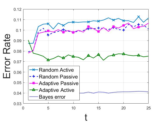
Figure 1: Experiments on synthetic regression: (a) Excess risk. (b) Estimated rate of change of minimizers. (c) Number of samples. Experiments on user preference tracking performance using Yelp data: (d) Excess risk. (e) Estimated rate of change of minimizers. (f) Classification error.

5.2 Tracking User Preferences in Recommendation System

We utilize a subset of Yelp 2017 dataset 22 2 https://www.yelp.com/dataset to perform our experiments. We censor the original dataset such that each user has at least 10 ratings. After censoring procedure, our dataset contains ratings of M=473M=473 users for N=858N=858 businesses. By converting the original 5-scale ratings to a binary label for all businesses with high ratings (4 and 5) as positive (11) and low ratings (3 and below) as negative (−1-1), we form the N×MN\times M binary rating matrix RR, which is very sparse and only 2.6%2.6\% are observed. We complete the sparse matrix RR to make recommendations by using the matrix factorization method [12]. The rating matrix RR can be modeled by the following logistic regression model

p⁡(Ru,b|ϕb,ϕu)=11+exp−Ru,b​ϕu⊤​ϕb,p(R_{u,b}|\phi_{b},\phi_{u})=\frac{1}{1+\exp^{-R_{u,b}\phi_{u}^{\top}\phi_{b}}}, (19)

where ϕu\phi_{u} and ϕb\phi_{b} are the dd-dimensional latent vectors representing the preferences of user uu and properties of business bb, respectively. Then, we train ϕu\phi_{u} and ϕb\phi_{b} with dimension d=5d=5 for each user and business in the dataset using maximum likelihood estimation by SGD. With the learned latent vectors, we can complete the matrix RR and make recommendations to customers in a collaborative filtering fashion [9, 15].

In practice, the preferences of users ϕu,t\phi_{u,t} may vary with time tt, and hence user features need to be retrained. Considering the fact that acquiring new ratings of users can be expensive, we apply our active and adaptive learning algorithm to further reduce the number of new samples while maintaining the mean tracking accuracy.

In the following experiment, we use a random subset of {ϕb}\{\phi_{b}\} with size NtN_{t} as our unlabeled data pool, while the remaining serve as a test set to evaluate the algorithms. To model the bounded time-varying changes of user preferences ϕu,t\phi_{u,t}, we start from a randomly chosen user feature and update it by adding a random Normal drift with norm bounded by 0.1 at each time step. Since we are unable to retrieve the actual answer from a real user, we generate the labels with the probabilistic model given by (19) with true parameter ϕu,t\phi_{u,t} instead. Note that one cannot ask a user the same question twice in a real recommendation system, and therefore we implement without replacement sampling by querying the labels of the samples having the largest Kt∗K_{t}^{*} values in the active sampling distribution Γ¯t\bar{\Gamma}_{t}.

Fig. 1 shows that ρ^t\hat{\rho}_{t} converges to a conservative estimate of ρ\rho, and the corresponding sample size converges to Kt∗=13K_{t}^{*}=13 after two time steps. Fig. 1 and Fig. 1 show that our algorithm achieves a error rate of 6% with these samples and significantly outperforms the other algorithms. This is because the Hessian matrices of logistic regression are functions of θt\theta_{t}, and hence the sampling distribution generated by the active and adaptive algorithm selects more informative samples.

6 Conclusions

In this paper, we propose an active and adaptive learning framework to solve a sequence of learning problems, which ensures a bounded excess risk for each individual learning task when the number of time steps is sufficiently large. We construct an estimator of the change in the minimizers ρ^t\hat{\rho}_{t} using active learning samples and show that this estimate upper bounds the true parameter ρ\rho almost surely. We test our algorithm on a synthetic regression problem, and further apply it to a recommendation system that tracks changes in preferences of customers. Our experiments demonstrate that our algorithm achieves better performance compared to the other baseline algorithms.

References

  • [1] A. Agarwal, A. Rakhlin, and P. Bartlett. Matrix regularization techniques for online multitask learning. Technical Report UCB/EECS-2008-138, EECS Department, University of California, Berkeley, 2008.
  • [2] A. Agarwal, S. Gerber, and H. Daume. Learning multiple tasks using manifold regularization. In Advances in Neural Information Processing Systems 23, pages 46–54, 2010.
  • [3] R G Antonini and Yu V Kozachenko. A note on the asymptotic behavior of sequences of generalized subgaussian random vectors. Random Operators and Stochastic Equations, 13(1):39–52, 2005.
  • [4] M.-F. Balcan, A. Beygelzimer, and J. Langford. Agnostic active learning. In Proceedings of the 23rd international conference on Machine learning, pages 65–72. ACM, 2006.
  • [5] O. Cappé, R. Douc, A. Guillin, J. Marin, and C. P Robert. Adaptive importance sampling in general mixture classes. Statistics and Computing, 18(4):447–459, 2008.
  • [6] K. Chaudhuri, S. M Kakade, P. Netrapalli, and S. Sanghavi. Convergence rates of active learning for maximum likelihood estimation. In Advances in Neural Information Processing Systems 28, pages 1090–1098, 2015.
  • [7] J. A Cornell. Experiments with mixtures: designs, models, and the analysis of mixture data. John Wiley & Sons, 2011.
  • [8] S. Dasgupta. Coarse sample complexity bounds for active learning. In Advances in Neural Information Processing Systems 18, pages 235–242, 2006.
  • [9] M. Elahi, F. Ricci, and N. Rubens. A survey of active learning in collaborative filtering recommender systems. Computer Science Review, 20:29–50, 2016.
  • [10] T. Evgeniou and M. Pontil. Regularized multi–task learning. In Proceedings of the 10th ACM SIGKDD international conference on Knowledge discovery and data mining, pages 109–117, 2004.
  • [11] R. Frostig, R. Ge, S. M Kakade, and A. Sidford. Competing with the empirical risk minimizer in a single pass. In Conference on Learning Theory, pages 728–763, 2015.
  • [12] Y. Koren, R. Bell, and C. Volinsky. Matrix factorization techniques for recommender systems. Computer, 42(8), 2009.
  • [13] M. Mohri, A. Rostamizadeh, and A. Talwalkar. Foundations of machine learning. MIT press, 2012.
  • [14] S. J Pan and Q. Yang. A survey on transfer learning. IEEE Transactions on Knowledge and Data Engineering, 22(10):1345–1359, 2010.
  • [15] N. Rubens, M. Elahi, M. Sugiyama, and D. Kaplan. Active learning in recommender systems. In Recommender Systems Handbook, pages 809–846. Springer, 2015.
  • [16] J. Sourati, M. Akcakaya, T. K Leen, D. Erdogmus, and J. G Dy. Asymptotic analysis of objectives based on fisher information in active learning. Journal of Machine Learning Research, 18(34):1–41, 2017.
  • [17] Zaid J Towfic, Jianshu Chen, and Ali H Sayed. On distributed online classification in the midst of concept drifts. Neurocomputing, 112:138–152, 2013.
  • [18] A. W Van der Vaart. Asymptotic statistics. Cambridge series in statistical and probabilistic mathematics. Cambridge University Press, 2000.
  • [19] C. Wilson and V. V Veeravalli. Adaptive sequential optimization with applications to machine learning. In Proceedings of IEEE International Conference on Acoustics, Speech and Signal Processing, pages 2642–2646, 2016.
  • [20] C. Wilson, V. V Veeravalli, and A. Nedich. Adaptive sequential stochastic optimization. IEEE Transactions on Automatic Control, 2018.
  • [21] Y. Zhang and D. Yeung. A convex formulation for learning task relationships in multi-task learning. arXiv preprint arXiv:1203.3536, 2012.

Appendix A Proof of Lemma 1

To prove Lemma 1, we use the following result from [11]. In particular, the following lemma is a generalization of Theorem 5.1 in [11], and its proof follows from generalizing the derivation of that theorem and is omitted here.

Lemma 3.

Suppose ψ1​(θ),⋯,ψK​(θ):ℝd→ℝ\psi_{1}(\theta),\cdots,\psi_{K}(\theta):\mathbb{R}^{d}\to\mathbb{R} are random functions drawn i.i.d. from a distribution, where θ∈Θ⊆ℝd\theta\in\Theta\subseteq\mathbb{R}^{d}. Denote P⁡(θ)=𝔼⁡[ψ⁡(θ)]P(\theta)=\mathbb{E}[\psi(\theta)] and let Q⁡(θ):ℝd→ℝQ(\theta):\mathbb{R}^{d}\to\mathbb{R} be another function. Let

θ^=argminθ∈Θ∑k=1Kψk(θ),andθ∗=argminθ∈ΘP(θ).\hat{\theta}=\argmin_{\theta\in\Theta}\sum_{k=1}^{K}\psi_{k}(\theta),\quad\mbox{and}\ \theta^{*}=\argmin_{\theta\in\Theta}P(\theta).

Assume:

  1. 1.

    Regularity conditions:

    1. (a)

      Compactness: Θ\Theta is compact, and θ∗\theta^{*} is an interior point of Θ\Theta.

    2. (b)

      Smoothness: ψ⁡(θ)\psi(\theta) is smooth in the following sense: the first, second and third derivatives exist at all interior points of Θ\Theta with probability one.

    3. (c)

      Convexity: ψ⁡(θ)\psi(\theta) is convex with probability one, and ∇2P​(θ∗)\nabla^{2}P(\theta^{*}) is positive definite.

    4. (d)

      ∇P​(θ∗)=0\nabla P(\theta^{*})=0 and ∇Q​(θ∗)=0\nabla Q(\theta^{*})=0.

  2. 2.

    Concentration at θ∗\theta^{*}: Suppose

    ∥∇ψ(θ∗)∥∇2P​(θ∗)−1≤L1′and∥(∇2P(θ∗))−1/2∇2ψ(θ∗)(∇2P(θ∗))−1/2∥2≤L2′\Big\|\nabla\psi(\theta^{*})\Big\|_{\nabla^{2}P(\theta^{*})^{-1}}\leq L_{1}^{\prime}\quad\mbox{and}\quad\Big\|\big(\nabla^{2}P(\theta^{*})\big)^{-1/2}\nabla^{2}\psi(\theta^{*})\big(\nabla^{2}P(\theta^{*})\big)^{-1/2}\Big\|_{2}\leq L_{2}^{\prime}

    hold with probability one.

  3. 3.

    Lipschitz continuity: There exists a neighborhood BB of θ∗\theta^{*} and a constant L3′L_{3}^{\prime}, such that ∇2ψ​(θ)\nabla^{2}\psi(\theta) and ∇2Q​(θ)\nabla^{2}Q(\theta) are L3′L_{3}^{\prime}-Lipschitz in this neighborhood, namely,

    ∥(∇2P(θ∗))−1/2(∇2ψ(θ)−∇2ψ(θ′))(∇2P(θ∗))−1/2∥2≤L3′∥θ−θ′∥∇2P​(θ∗),∥(∇2Q(θ∗))−1/2(∇2Q(θ)−∇2Q(θ′))(∇2Q(θ∗))−1/2∥2≤L3′∥θ−θ′∥∇2P​(θ∗),\begin{split}&\Big\|\big(\nabla^{2}P(\theta^{*})\big)^{-1/2}\big(\nabla^{2}\psi(\theta)-\nabla^{2}\psi(\theta^{\prime})\big)\big(\nabla^{2}P(\theta^{*})\big)^{-1/2}\Big\|_{2}\leq L_{3}^{\prime}\|\theta-\theta^{\prime}\|_{\nabla^{2}P(\theta^{*})},\\ &\Big\|\big(\nabla^{2}Q(\theta^{*})\big)^{-1/2}\big(\nabla^{2}Q(\theta)-\nabla^{2}Q(\theta^{\prime})\big)\big(\nabla^{2}Q(\theta^{*})\big)^{-1/2}\Big\|_{2}\leq L_{3}^{\prime}\|\theta-\theta^{\prime}\|_{\nabla^{2}P(\theta^{*})},\end{split}

    holds with probability one, for θ,θ′∈B\theta,\theta^{\prime}\in B,

Choose p≥2p\geq 2 and define

γ≜c⁡(L1′​L3′+L2′)​p​log⁡d​KK,\gamma\triangleq c(L_{1}^{\prime}L_{3}^{\prime}+\sqrt{L_{2}^{\prime}})\sqrt{{\frac{p\log dK}{K}}},

where cc is an appropriately chosen constant. Let c′c^{\prime} be another appropriately chosen constant. If KK is large enough so that p​log⁡d​KK≤c′​min⁡{1L2′,1L1′​L3′,diameter⁡(B)L1′}\sqrt{\frac{p\log dK}{K}}\leq c^{\prime}\min\left\{\frac{1}{\sqrt{L_{2}^{\prime}}},\frac{1}{L_{1}^{\prime}L_{3}^{\prime}},\frac{\mathrm{diameter}(B)}{L_{1}^{\prime}}\right\}, then:

(1−γ)​τ2K−L1′2Kp/2≤𝔼⁡[Q⁡(θ^)−Q⁡(θ∗)]≤(1+γ)​τ2K+maxθ∈Θ⁡[Q⁡(θ)−Q⁡(θ∗)]Kp,(1-\gamma)\frac{\tau^{2}}{K}-\frac{L_{1}^{\prime 2}}{K^{p/2}}\leq\mathbb{E}\big[Q(\hat{\theta})-Q(\theta^{*})\big]\leq(1+\gamma)\frac{\tau^{2}}{K}+\frac{\max_{\theta\in\Theta}\left[Q(\theta)-Q(\theta^{*})\right]}{K^{p}},

where

τ2≜12​K2Tr(∑i,j𝔼[∇ψi(θ∗)∇ψj(θ∗)⊤](∇2P(θ∗))−1∇2Q(θ∗)(∇2P(θ∗))−1).\tau^{2}\triangleq\frac{1}{2K^{2}}{\mathrm{Tr}}\bigg(\sum_{i,j}\mathbb{E}\big[\nabla\psi_{i}(\theta^{*})\nabla\psi_{j}(\theta^{*})^{\top}\big]\big(\nabla^{2}P(\theta^{*})\big)^{-1}\nabla^{2}Q(\theta^{*})\big(\nabla^{2}P(\theta^{*})\big)^{-1}\bigg).

Then, we proceed to prove Lemma 1.

Proof of Lemma 1.

We first use Lemma 3 to bound the excess risk, which is similar to the idea of Lemma 1 in [6]. We first define

ψk​(θt)=ℓ⁡(Yk,t|Xk,t,θt),\psi_{k}(\theta_{t})=\ell(Y_{k,t}|X_{k,t},\theta_{t}), (20)

where Xk,t∼ΓtX_{k,t}\sim\Gamma_{t} and Yk,t∼p⁡(Yk,t|Xk,t,θt∗)Y_{k,t}\sim p(Y_{k,t}|X_{k,t},\theta_{t}^{*}) for 1≤k≤Kt1\leq k\leq K_{t}. Then,

P⁡(θt)=𝔼⁡(ψk​(θt))=LΓt​(θt),and∇2P​(θt∗)=IΓt​(θt∗).P(\theta_{t})=\mathbb{E}(\psi_{k}(\theta_{t}))=L_{\Gamma_{t}}(\theta_{t}),\quad\mbox{and}\quad\nabla^{2}P(\theta_{t}^{*})=I_{\Gamma_{t}}(\theta_{t}^{*}). (21)

Further, we choose

Q⁡(θt)=LUt​(θt),and∇2Q​(θt∗)=IUt​(θt∗).Q(\theta_{t})=L_{U_{t}}(\theta_{t}),\quad\mbox{and}\quad\nabla^{2}Q(\theta_{t}^{*})=I_{U_{t}}(\theta_{t}^{*}). (22)

As shown in Assumption 2, the assumptions of Lemma 3 are satisfied. Moreover, according to the condition that IΓt​(θ∗)⪰C​IUt​(θ∗)I_{\Gamma_{t}}(\theta^{*})\succeq CI_{U_{t}}(\theta^{*}) holds for some constant C<1C<1 in Lemma 1, we have

∥IΓt(θt∗)−1/2\displaystyle\Big\|I_{\Gamma_{t}}(\theta_{t}^{*})^{-1/2} (H(x,θt)−H(x,θt′))IΓt(θt∗)−1/2∥2\displaystyle\big(H(x,\theta_{t})-H(x,\theta_{t}^{\prime})\big)I_{\Gamma_{t}}(\theta_{t}^{*})^{-1/2}\Big\|_{2}
≤1C∥IUt(θt∗)−1/2(H(x,θt)−H(x,θt′))IUt(θt∗)−1/2∥2\displaystyle\leq\frac{1}{C}\Big\|I_{U_{t}}(\theta_{t}^{*})^{-1/2}\big(H(x,\theta_{t})-H(x,\theta_{t}^{\prime})\big)I_{U_{t}}(\theta_{t}^{*})^{-1/2}\Big\|_{2}
≤L3C​‖θ−θ′‖IUt​(θt∗)≤L3C3/2​‖θ−θ′‖IΓt​(θt∗)\displaystyle\leq\frac{L_{3}}{C}\|\theta-\theta^{\prime}\|_{I_{U_{t}}(\theta_{t}^{*})}\leq\frac{L_{3}}{C^{3/2}}\|\theta-\theta^{\prime}\|_{I_{\Gamma_{t}}(\theta_{t}^{*})} (23)

and

∥IUt(θt∗)−1/2\displaystyle\Big\|I_{U_{t}}(\theta_{t}^{*})^{-1/2} (H(x,θt)−H(x,θt′))IUt(θt∗)−1/2∥2\displaystyle\big(H(x,\theta_{t})-H(x,\theta_{t}^{\prime})\big)I_{U_{t}}(\theta_{t}^{*})^{-1/2}\Big\|_{2}
≤L3​‖θ−θ′‖IUt​(θt∗)≤L3C​‖θ−θ′‖IΓt​(θt∗).\displaystyle\leq L_{3}\|\theta-\theta^{\prime}\|_{I_{U_{t}}(\theta_{t}^{*})}\leq\frac{L_{3}}{\sqrt{C}}\|\theta-\theta^{\prime}\|_{I_{\Gamma_{t}}(\theta_{t}^{*})}. (24)

Hence, L3′=max⁡{L3/C3/2,L3/C}=L3/C3/2L_{3}^{\prime}=\max\{{L_{3}}/{C^{3/2}},{L_{3}}/{\sqrt{C}}\}={L_{3}}/{C^{3/2}}. Similarly, we have L1′=L1/CL_{1}^{\prime}={L_{1}}/{\sqrt{C}} and L2′=L2/CL_{2}^{\prime}={L_{2}}/{C}. In summary, the Assumptions 2 and 3 in Lemma 3 are satisfied with constants

(L1′,L2′,L3′)=(L1/C,L2/C,L3/C3/2).(L_{1}^{\prime},L_{2}^{\prime},L_{3}^{\prime})=(L_{1}/\sqrt{C},L_{2}/C,L_{3}/C^{3/2}). (25)

Applying Lemma 3 with p=2p=2 and considering the fact that 𝔼x∼Γt[∇ℓ(Yi,t|Xi,t,θt∗)∇ℓ(Yi,t|Xi,t,θt∗)⊤]=IΓt(θt∗)\mathbb{E}_{x\sim\Gamma_{t}}\big[\nabla\ell(Y_{i,t}|X_{i,t},\theta_{t}^{*})\nabla\ell(Y_{i,t}|X_{i,t},\theta_{t}^{*})^{\top}\big]=I_{\Gamma_{t}}(\theta_{t}^{*}),

(1−γt)​τt2Kt−L12C​Kt2≤𝔼⁡[LUt​(θ^Γt)−LUt​(θt∗)]≤(1+γt)​τt2Kt+maxθ∈Θt⁡[LUt​(θ)−LUt​(θt∗)]Kt2(1-\gamma_{t})\frac{\tau_{t}^{2}}{K_{t}}-\frac{L_{1}^{2}}{CK_{t}^{2}}\leq\mathbb{E}\big[L_{U_{t}}(\hat{\theta}_{\Gamma_{t}})-L_{U_{t}}(\theta_{t}^{*})\big]\leq(1+\gamma_{t})\frac{\tau_{t}^{2}}{K_{t}}+\frac{\max_{\theta\in\Theta_{t}}\left[L_{U_{t}}(\theta)-L_{U_{t}}(\theta_{t}^{*})\right]}{K_{t}^{2}} (26)

holds, where

γt=𝒪⁡((L1′​L3′+L2′)​log⁡d​KtKt)=𝒪⁡(1C2​(L1​L3+L2)​log⁡d​KtKt),\gamma_{t}=\mathcal{O}\bigg((L_{1}^{\prime}L_{3}^{\prime}+\sqrt{L_{2}^{\prime}})\sqrt{\frac{\log dK_{t}}{K_{t}}}\bigg)=\mathcal{O}\bigg(\frac{1}{C^{2}}(L_{1}L_{3}+\sqrt{L_{2}})\sqrt{\frac{\log dK_{t}}{K_{t}}}\bigg), (27)

and τt2=12​Tr​((IΓt​(θt∗))−1​IUt​(θt∗))\tau_{t}^{2}=\frac{1}{2}{\mathrm{Tr}}\Big(\big(I_{\Gamma_{t}}(\theta_{t}^{*})\big)^{-1}I_{U_{t}}(\theta_{t}^{*})\Big).

Note that if we assume the parameter set Θt≜{θt|‖θt−θt−1∗‖≤ρ}\Theta_{t}\triangleq\{\theta_{t}|\|\theta_{t}-\theta_{t-1}^{*}\|\leq\rho\} is known, then the second term in the right hand side of (26) can be further bounded as

maxθ∈Θt⁡[LUt​(θ)−LUt​(θt∗)]Kt2≤maxθ∈Θt⁡[Lb​‖θ−θt∗‖2]2​Kt2≤Lb​Diameter​(Θt)22​Kt2≤2​Lb​ρ2Kt2,\frac{\max_{\theta\in\Theta_{t}}\left[L_{U_{t}}(\theta)-L_{U_{t}}(\theta_{t}^{*})\right]}{K_{t}^{2}}\leq\frac{\max_{\theta\in\Theta_{t}}\left[L_{b}\|\theta-\theta_{t}^{*}\|^{2}\right]}{2K_{t}^{2}}\leq\frac{L_{b}\mathrm{Diameter}(\Theta_{t})^{2}}{2K_{t}^{2}}\leq\frac{2L_{b}\rho^{2}}{K_{t}^{2}}, (28)

where the inequalities follow from the boundedness condition in Assumption 2. Combining this result with the inequality in (26) completes the proof of Lemma 1. ∎

Appendix B Proof of Theorem 1

Proof of Theorem 1.

The proof starts from the bound b⁡(τ2,Δt,Kt)b(\tau^{2},\Delta_{t},K_{t}) of the SGD algorithm in Assumption 4. To compute the convergence rate τ2\tau^{2}, we need to first study the approximation of θt∗\theta_{t}^{*} using θ^t−1\hat{\theta}_{t-1}. The difference between θ^t−1\hat{\theta}_{t-1} and θt∗\theta_{t}^{*} can be bounded as

‖θ^t−1−θt∗‖2≤‖θt−1∗−θt∗‖2+‖θ^t−1−θt−1∗‖2≤ρ+‖θ^t−1−θt−1∗‖2.\big\|\hat{\theta}_{t-1}-\theta_{t}^{*}\big\|_{2}\leq\big\|\theta_{t-1}^{*}-\theta_{t}^{*}\big\|_{2}+\big\|\hat{\theta}_{t-1}-\theta_{t-1}^{*}\big\|_{2}\leq\rho+\big\|\hat{\theta}_{t-1}-\theta_{t-1}^{*}\big\|_{2}. (29)

To bound the second term, we use the strongly convexity assumption in Assumption 2,

‖θ^t−1−θt−1∗‖22≤2m​(LUt−1​(θ^t−1)−LUt−1​(θt−1∗)).\big\|\hat{\theta}_{t-1}-\theta_{t-1}^{*}\big\|_{2}^{2}\leq\frac{2}{m}(L_{U_{t-1}}\big(\hat{\theta}_{t-1})-L_{U_{t-1}}({\theta}_{t-1}^{*})\big). (30)

Suppose the excess risk bound 𝔼⁡[LUt−1​(θ^t−1)−LUt−1​(θt−1∗)]≤ε\mathbb{E}[L_{U_{t-1}}(\hat{\theta}_{t-1})-L_{U_{t-1}}({\theta}_{t-1}^{*})]\leq\varepsilon holds for t−1t-1. Then, we have

𝔼⁡(‖θ^t−1−θt−1∗‖2)≤𝔼⁡(‖θ^t−1−θt−1∗‖22)≤2​ε/m.\mathbb{E}(\big\|\hat{\theta}_{t-1}-\theta_{t-1}^{*}\big\|_{2})\leq\sqrt{\mathbb{E}(\big\|\hat{\theta}_{t-1}-\theta_{t-1}^{*}\big\|_{2}^{2})}\leq\sqrt{{2\varepsilon}/{m}}. (31)

Then, ‖θ^t−1−θt−1∗‖2≤1δ​2​εm\big\|\hat{\theta}_{t-1}-\theta_{t-1}^{*}\big\|_{2}\leq\frac{1}{\delta}\sqrt{\frac{2\varepsilon}{m}} holds with probability 1−δ1-\delta by Markov’s inequality, for ∀δ∈(0,1)\forall\delta\in(0,1). Thus,

‖θ^t−1−θt∗‖2≤ρ+1δ​2​εm\big\|\hat{\theta}_{t-1}-\theta_{t}^{*}\big\|_{2}\leq\rho+\frac{1}{\delta}\sqrt{\frac{2\varepsilon}{m}} (32)

holds with probability 1−δ1-\delta. By the self-concordance condition in Assumption 3, we have that

(1−βt)​H​(xt,θt∗)⪯H⁡(xt,θ^t−1)⪯(1+βt)​H​(xt,θt∗),xt∈𝒮t,(1-\beta_{t})H(x_{t},\theta_{t}^{*})\preceq H(x_{t},\hat{\theta}_{t-1})\preceq(1+\beta_{t})H(x_{t},\theta_{t}^{*}),\quad x_{t}\in\mathcal{S}_{t}, (33)

holds with probability 1−δ1-\delta, where βt=L4​(ρ+1δ​2​εm)\beta_{t}=L_{4}(\rho+\frac{1}{\delta}\sqrt{\frac{2\varepsilon}{m}}). Then, for distribution Γt∗\Gamma_{t}^{*}, Γ^t∗\hat{\Gamma}_{t}^{*} and UtU_{t}, we have

(1−βt)​IΓt∗​(θt∗)⪯IΓt∗​(θ^t−1)⪯(1+βt)​IΓt∗​(θt∗),(1-\beta_{t})I_{\Gamma_{t}^{*}}(\theta_{t}^{*})\preceq I_{\Gamma_{t}^{*}}(\hat{\theta}_{t-1})\preceq(1+\beta_{t})I_{\Gamma_{t}^{*}}(\theta_{t}^{*}), (34)
(1−βt)​IΓ^t∗​(θt∗)⪯IΓ^t∗​(θ^t−1)⪯(1+βt)​IΓ^t∗​(θt∗),(1-\beta_{t})I_{\hat{\Gamma}_{t}^{*}}(\theta_{t}^{*})\preceq I_{\hat{\Gamma}_{t}^{*}}(\hat{\theta}_{t-1})\preceq(1+\beta_{t})I_{\hat{\Gamma}_{t}^{*}}(\theta_{t}^{*}), (35)
(1−βt)​IUt​(θt∗)⪯IUt​(θ^t−1)⪯(1+βt)​IUt​(θt∗).(1-\beta_{t})I_{U_{t}}(\theta_{t}^{*})\preceq I_{U_{t}}(\hat{\theta}_{t-1})\preceq(1+\beta_{t})I_{U_{t}}(\theta_{t}^{*}). (36)

Recall that Γ¯t=αt​Γ^t∗+(1−αt)​Ut\bar{\Gamma}_{t}=\alpha_{t}\hat{\Gamma}_{t}^{*}+(1-\alpha_{t})U_{t}. Hence, IΓ¯t​(θt∗)⪰αt​IΓ^t∗​(θt∗)I_{\bar{\Gamma}_{t}}(\theta_{t}^{*})\succeq\alpha_{t}I_{\hat{\Gamma}_{t}^{*}}(\theta_{t}^{*}) which implies that IΓ¯t​(θt∗)−1⪯1αt​IΓ^t​(θt∗)−1I_{\bar{\Gamma}_{t}}(\theta_{t}^{*})^{-1}\preceq\frac{1}{\alpha_{t}}I_{\hat{\Gamma}_{t}}(\theta_{t}^{*})^{-1}. Thus,

τt2=12​Tr​(IΓ¯t−1​(θt∗)​IUt​(θt∗))≤12​αt​Tr​(IΓ^t∗−1​(θt∗)​IUt​(θt∗)).\tau_{t}^{2}=\frac{1}{2}\mathrm{Tr}\big(I_{\bar{\Gamma}_{t}}^{-1}(\theta_{t}^{*})I_{U_{t}}(\theta_{t}^{*})\big)\leq\frac{1}{2\alpha_{t}}\mathrm{Tr}\big(I_{\hat{\Gamma}_{t}^{*}}^{-1}(\theta_{t}^{*})I_{U_{t}}(\theta_{t}^{*})\big). (37)

From (35) and (36), (37) can be further upper bounded by

Tr⁡(IΓ^t∗−1​(θt∗)​IUt​(θt∗))\displaystyle\mathrm{Tr}\big(I_{\hat{\Gamma}_{t}^{*}}^{-1}(\theta_{t}^{*})I_{U_{t}}(\theta_{t}^{*})\big) ≤1+βt1−βt​Tr​(IΓ^t∗−1​(θ^t−1)​IUt​(θ^t−1))\displaystyle\leq\frac{1+\beta_{t}}{1-\beta_{t}}{\mathrm{Tr}}\big(I_{\hat{\Gamma}_{t}^{*}}^{-1}(\hat{\theta}_{t-1})I_{U_{t}}(\hat{\theta}_{t-1})\big)
≤(a)​1+βt1−βt​Tr​(IΓt∗−1​(θ^t−1)​IUt​(θ^t−1))\displaystyle\overset{(a)}{\leq}\frac{1+\beta_{t}}{1-\beta_{t}}{\mathrm{Tr}}\big(I_{\Gamma_{t}^{*}}^{-1}(\hat{\theta}_{t-1})I_{U_{t}}(\hat{\theta}_{t-1})\big)
≤(b)​(1+βt1−βt)2​Tr​(IΓt∗−1​(θt∗)​IUt​(θt∗)),\displaystyle\overset{(b)}{\leq}\left(\frac{1+\beta_{t}}{1-\beta_{t}}\right)^{2}{\mathrm{Tr}}\big(I_{\Gamma_{t}^{*}}^{-1}(\theta_{t}^{*})I_{U_{t}}(\theta_{t}^{*})\big), (38)

where (a) is because that Γ^t∗\hat{\Gamma}_{t}^{*} is the minimizer of Tr⁡(IΓt−1​(θ^t−1)​IUt​(θ^t−1)){\mathrm{Tr}}\big(I_{{\Gamma}_{t}}^{-1}(\hat{\theta}_{t-1})I_{U_{t}}(\hat{\theta}_{t-1})\big) and (b) follows from the results in (34) and (36).

To bound the difference between the initialization and the true minimizer, we use triangle inequality and Jensen’s inequality to get

𝔼​‖θ^t−1−θt∗‖22≤𝔼​‖θ^t−1−θt−1∗‖22+‖θt∗−θt−1∗‖≤𝔼​‖θ^t−1−θt−1∗‖22+ρ.\sqrt{\mathbb{E}\|\hat{\theta}_{t-1}-\theta_{t}^{*}\|_{2}^{2}}\leq\sqrt{\mathbb{E}\|\hat{\theta}_{t-1}-\theta_{t-1}^{*}\|_{2}^{2}}+\|\theta_{t}^{*}-\theta_{t-1}^{*}\|\leq\sqrt{\mathbb{E}\|\hat{\theta}_{t-1}-\theta_{t-1}^{*}\|_{2}^{2}}+\rho. (39)

From (31), we have

𝔼​‖θ^t−1−θt−1∗‖22≤2​εm,\mathbb{E}\|\hat{\theta}_{t-1}-\theta_{t-1}^{*}\|_{2}^{2}\leq\frac{2\varepsilon}{m}, (40)

which yields

𝔼​‖θ^t−1−θt∗‖22≤(2​εm+ρ)2=Δt2.\mathbb{E}\|\hat{\theta}_{t-1}-\theta_{t}^{*}\|_{2}^{2}\leq\Big(\sqrt{\frac{2\varepsilon}{m}}+\rho\Big)^{2}=\Delta_{t}^{2}. (41)

Thus, combining the above result with the bound in (38), we can conclude that the following upper bound

𝔼⁡[LUt​(θ^t)−LUt​(θt∗)]≤b⁡(τ´t2,Δt,Kt),\mathbb{E}[L_{U_{t}}(\hat{\theta}_{t})-L_{U_{t}}(\theta_{t}^{*})]\leq b(\acute{\tau}_{t}^{2},\Delta_{t},K_{t}), (42)

holds with probability 1-δ\delta, where

τ´t2=(1+βt1−βt)2​Tr⁡(IΓt∗−1​(θt∗)​IUt​(θt∗))2​αt.\acute{\tau}_{t}^{2}=\Big(\frac{1+\beta_{t}}{1-\beta_{t}}\Big)^{2}\frac{\mathrm{Tr}\big(I_{\Gamma_{t}^{*}}^{-1}(\theta_{t}^{*})I_{U_{t}}(\theta_{t}^{*})\big)}{2\alpha_{t}}. (43)

This completes the proof of Theorem 1.

∎

Appendix C Proof of Lemma 2

Proof of Lemma 2.

The following inequalities hold from the strong convexity assumption and the fact that ∇LUt​(θt∗)=∇LUt−1​(θt−1∗)=0\nabla L_{U_{t}}(\theta^{*}_{t})=\nabla L_{U_{t-1}}(\theta^{*}_{t-1})=0:

LUt​(θt−1∗)\displaystyle L_{U_{t}}(\theta^{*}_{t-1}) ≥LUt​(θt∗)+12​m​‖θt∗−θt−1∗‖22\displaystyle\geq L_{U_{t}}(\theta^{*}_{t})+\frac{1}{2}m\|\theta_{t}^{*}-\theta_{t-1}^{*}\|_{2}^{2} (44)
LUt−1​(θt∗)\displaystyle L_{U_{t-1}}(\theta^{*}_{t}) ≥LUt−1​(θt−1∗)+12​m​‖θt∗−θt−1∗‖22.\displaystyle\geq L_{U_{t-1}}(\theta^{*}_{t-1})+\frac{1}{2}m\|\theta_{t}^{*}-\theta_{t-1}^{*}\|_{2}^{2}. (45)

Then, adding and rearranging these inequalities yields

1m\displaystyle\frac{1}{m} [LUt​(θt−1∗)−LUt​(θt∗)+LUt−1​(θt∗)−LUt−1​(θt−1∗)]≥‖θt∗−θt−1∗‖22.\displaystyle\Big[L_{U_{t}}(\theta^{*}_{t-1})-L_{U_{t}}(\theta^{*}_{t})+L_{U_{t-1}}(\theta^{*}_{t})-L_{U_{t-1}}(\theta^{*}_{t-1})\Big]\geq\|\theta_{t}^{*}-\theta_{t-1}^{*}\|_{2}^{2}. (46)

∎

Moreover, we have the following relation

∥θt∗\displaystyle\|\theta_{t}^{*} −θt−1∗∥22\displaystyle-\theta_{t-1}^{*}\|_{2}^{2}
≤1m​[LUt​(θt−1∗)−LUt​(θt∗)+LUt−1​(θt∗)−LUt−1​(θt−1∗)]\displaystyle\leq\frac{1}{m}\Big[L_{U_{t}}(\theta^{*}_{t-1})-L_{U_{t}}(\theta^{*}_{t})+L_{U_{t-1}}(\theta^{*}_{t})-L_{U_{t-1}}(\theta^{*}_{t-1})\Big]
=1m[𝔼X∼Ut[D(p(Y|X,θt∗)∥p(Y|X,θt−1∗))]+𝔼X∼Ut−1[D(p(Y|X,θt−1∗)∥p(Y|X,θt∗))]],\displaystyle=\frac{1}{m}\Big[\mathbb{E}_{X\sim U_{t}}\big[D\big(p(Y|X,\theta_{t}^{*})\|p(Y|X,\theta_{t-1}^{*})\big)\big]+\mathbb{E}_{X\sim U_{t-1}}\big[D\big(p(Y|X,\theta_{t-1}^{*})\|p(Y|X,\theta_{t}^{*})\big)\big]\Big], (47)

where

D(p∥q)≜∫y∈𝒴p(y)logp⁡(y)q⁡(y)dyD(p\|q)\triangleq\int_{y\in\mathcal{Y}}p(y)\log\frac{p(y)}{q(y)}dy (48)

is the KL divergence between distribution pp and qq.

Thus, an upper bound of ρ\rho can be constructed by estimating the symmetric KL divergence between p⁡(y|x,θt∗)p(y|x,\theta_{t}^{*}) and p⁡(y|x,θt−1∗)p(y|x,\theta_{t-1}^{*}) using the data pool UtU_{t} and Ut−1U_{t-1}, respectively.

Appendix D Proof of Theorem 3

To analyze the performance of the estimator of ρ\rho, we need to introduce a few results for sub-Gaussian random variables including the following key technical lemma from [3]. This lemma controls the concentration of sums of random variables that are sub-Gaussian conditioned on a particular filtration.

Lemma 4.

Suppose we have a collection of random variables {Vi}i=1n\{V_{i}\}_{i=1}^{n} and a filtration {ℱi}i=0n\{\mathscr{F}_{i}\}_{i=0}^{n} such that for each random variable ViV_{i} it holds that

  1. 1.

    𝔼⁡[exp⁡{s⁡(Vi−𝔼⁡[Vi|ℱi−1])}|ℱi−1]≤e12​σi2​s2\mathbb{E}[\exp\{s(V_{i}-\mathbb{E}[V_{i}|\mathscr{F}_{i-1}])\}|\mathscr{F}_{i-1}]\leq e^{\frac{1}{2}\sigma_{i}^{2}s^{2}} with σi2\sigma_{i}^{2} a constant.

  2. 2.

    ViV_{i} is ℱi\mathscr{F}_{i}-measurable.

Then for every 𝒂∈ℝn\text{\boldmath{$a$}}\in\mathbb{R}^{n} it holds that

ℙ{∑i=1naiVi>∑i=1nai𝔼[Vi|ℱi−1]+t}≤exp{t22​ν}\mathbb{P}\left\{\sum_{i=1}^{n}a_{i}V_{i}>\sum_{i=1}^{n}a_{i}\mathbb{E}[V_{i}|\mathscr{F}_{i-1}]+t\right\}\leq\exp\Big\{\frac{t^{2}}{2\nu}\Big\}

with ν=∑i=1nσi2​ai2\nu=\sum_{i=1}^{n}\sigma_{i}^{2}a_{i}^{2}. The other tail is similarly bounded.

If we can upper bound the conditional expectations 𝔼⁡[Vi|ℱi−1]≤ξi\mathbb{E}[V_{i}|\mathscr{F}_{i-1}]\leq\xi_{i} by some constants ξi\xi_{i}, then we have

ℙ{∑i=1naiVi>∑i=1naiξi+t}≤exp{t22​ν}.\mathbb{P}\left\{\sum_{i=1}^{n}a_{i}V_{i}>\sum_{i=1}^{n}a_{i}\xi_{i}+t\right\}\leq\exp\Big\{\frac{t^{2}}{2\nu}\Big\}. (49)

For our analysis, we generally cannot compute 𝔼⁡[Vi|ℱi−1]\mathbb{E}[V_{i}|\mathscr{F}_{i-1}] directly, but we can find the upper bound ξi\xi_{i}. To compute σi2\sigma_{i}^{2} for use in Lemma 4, we employ the following conditional version of Hoeffding’s Lemma.

Lemma 5.

(Conditional Hoeffding’s Lemma): If a random variable VV and a sigma algebra ℱ\mathscr{F} satisfy a≤V≤ba\leq V\leq b and E⁡[V|ℱ]=0E[V|\mathscr{F}]=0, then

𝔼⁡[es​V|ℱ]≤exp⁡{18​(b−a)2​s2}.\mathbb{E}[e^{sV}|\mathscr{F}]\leq\exp\Big\{\frac{1}{8}(b-a)^{2}s^{2}\Big\}.
Proof of Lemma Theorem 3.

To simplify our proof, we look at a special case where ‖θt∗−θt−1∗‖=ρ\|\theta_{t}^{*}-\theta_{t-1}^{*}\|=\rho holds. The proof for the case ‖θt∗−θt−1∗‖≤ρ\|\theta_{t}^{*}-\theta_{t-1}^{*}\|\leq\rho is similar, and more details about the window function hWh_{W} can be found in [20].

For the case ‖θt∗−θt−1∗‖=ρ\|\theta_{t}^{*}-\theta_{t-1}^{*}\|=\rho, we use the following estimator to combine the one-step estimator ρ~t\widetilde{\rho}_{t}

ρ´t2=1t−1​∑i=2tρ~i2=1m⁡(t−1)​∑i=2t(L^Ui​(θ^i−1)−L^Ui​(θ^i)+L^Ui−1​(θ^i)−L^Ui−1​(θ^i−1)).\acute{\rho}_{t}^{2}=\frac{1}{t-1}\sum_{i=2}^{t}\widetilde{\rho}_{i}^{2}=\frac{1}{m(t-1)}\sum_{i=2}^{t}\big(\hat{L}_{U_{i}}(\hat{\theta}_{i-1})-\hat{L}_{U_{i}}(\hat{\theta}_{i})+\hat{L}_{U_{i-1}}(\hat{\theta}_{i})-\hat{L}_{U_{i-1}}(\hat{\theta}_{i-1})\big). (50)

We denote

ρt2≜1m⁡(t−1)​∑i=2t(LUi​(θi−1∗)−LUi​(θi∗)+LUi−1​(θi∗)−LUi−1​(θi−1∗))≥ρ2.\rho_{t}^{2}\triangleq\frac{1}{m(t-1)}\sum_{i=2}^{t}\big(L_{U_{i}}(\theta_{i-1}^{*})-L_{U_{i}}(\theta_{i}^{*})+L_{U_{i-1}}(\theta_{i}^{*})-L_{U_{i-1}}(\theta_{i-1}^{*})\big)\geq\rho^{2}. (51)

where the inequality follows from Lemma 2. We want to construct ρ^t\hat{\rho}_{t}, such that ρ^t2≥ρt2≥ρ2\hat{\rho}_{t}^{2}\geq\rho_{t}^{2}\geq\rho^{2} almost surely. Then, we have

ρt2−ρ´t2=\displaystyle\rho_{t}^{2}-\acute{\rho}_{t}^{2}= 1m⁡(t−1)​(∑i=2tLUi​(θi−1∗)−L^Ui​(θ^i−1)+∑i=2tLUi−1​(θi∗)−L^Ui−1​(θ^i)CLOSE\displaystyle\frac{1}{m(t-1)}\Big(\sum_{i=2}^{t}L_{U_{i}}(\theta_{i-1}^{*})-\hat{L}_{U_{i}}(\hat{\theta}_{i-1})+\sum_{i=2}^{t}L_{U_{i-1}}(\theta_{i}^{*})-\hat{L}_{U_{i-1}}(\hat{\theta}_{i}) (52)
OPEN+L^U1​(θ^1)−LU1​(θ1∗)+2​∑i=2t−1L^Ui​(θ^i)−LUi​(θi∗)+L^Ut​(θ^t)−LUt​(θt∗)).\displaystyle\qquad+\hat{L}_{U_{1}}(\hat{\theta}_{1})-L_{U_{1}}(\theta_{1}^{*})+2\sum_{i=2}^{t-1}\hat{L}_{U_{i}}(\hat{\theta}_{i})-L_{U_{i}}(\theta_{i}^{*})+\hat{L}_{U_{t}}(\hat{\theta}_{t})-L_{U_{t}}(\theta_{t}^{*})\Big). (53)

Define

Ut\displaystyle U_{t} ≜1(t−1)​∑i=2t1m​(LUi​(θi−1∗)−L^Ui​(θ^i−1)),\displaystyle\triangleq\frac{1}{(t-1)}\sum_{i=2}^{t}\frac{1}{m}\big(L_{U_{i}}(\theta_{i-1}^{*})-\hat{L}_{U_{i}}(\hat{\theta}_{i-1})\big), (54)
Vt\displaystyle V_{t} ≜1(t−1)​∑i=2t1m​(LUi−1​(θi∗)−L^Ui−1​(θ^i)),\displaystyle\triangleq\frac{1}{(t-1)}\sum_{i=2}^{t}\frac{1}{m}\big(L_{U_{i-1}}(\theta_{i}^{*})-\hat{L}_{U_{i-1}}(\hat{\theta}_{i})\big), (55)
Wt\displaystyle W_{t} ≜1m⁡(t−1)​(L^U1​(θ^1)−LU1​(θ1∗)+2​∑i=2t−1(L^Ui​(θ^i)−LUi​(θi∗))+L^Ut​(θ^t)−LUt​(θt∗)).\displaystyle\triangleq\frac{1}{m(t-1)}\Big(\hat{L}_{U_{1}}(\hat{\theta}_{1})-L_{U_{1}}(\theta_{1}^{*})+2\sum_{i=2}^{t-1}\big(\hat{L}_{U_{i}}(\hat{\theta}_{i})-L_{U_{i}}(\theta_{i}^{*})\big)+\hat{L}_{U_{t}}(\hat{\theta}_{t})-L_{U_{t}}(\theta_{t}^{*})\Big). (56)

Then it holds that

ρt2−ρ´t2=Ut+Vt+Wt.\rho_{t}^{2}-\acute{\rho}_{t}^{2}=U_{t}+V_{t}+W_{t}. (57)

Now, we look at bounding 𝔼⁡[LUi​(θi−1∗)−L^Ui​(θ^i−1)]\mathbb{E}\big[L_{U_{i}}(\theta_{i-1}^{*})-\hat{L}_{U_{i}}(\hat{\theta}_{i-1})\big], 𝔼⁡[LUi−1​(θi∗)−L^Ui−1​(θ^i)]\mathbb{E}\big[L_{U_{i-1}}(\theta_{i}^{*})-\hat{L}_{U_{i-1}}(\hat{\theta}_{i})\big] and 𝔼⁡[L^Ui​(θ^i)−LUi​(θi∗)]\mathbb{E}\big[\hat{L}_{U_{i}}(\hat{\theta}_{i})-L_{U_{i}}(\theta_{i}^{*})\big] in UtU_{t}, VtV_{t} and WtW_{t}, respectively.

Note that, the samples at time step i−1i-1 are independent with samples at time ii, hence,

𝔼⁡[L^Ui​(θ^i−1)]\displaystyle\mathbb{E}\big[\hat{L}_{U_{i}}(\hat{\theta}_{i-1})\big] =𝔼⁡[𝔼Xk,i∼Γ¯i,Yk,i∼p⁡(Y|Xk,i,θi∗)​[1Ki​∑i=1Kiℓ⁡(Yk,i|Xk,i,θ^i−1)Ni​Γ¯i​(Xk,i)]]\displaystyle=\mathbb{E}\Big[\mathbb{E}_{X_{k,i}\sim\bar{\Gamma}_{i},Y_{k,i}\sim p(Y|X_{k,i},\theta_{i}^{*})}\big[\frac{1}{K_{i}}\sum_{i=1}^{K_{i}}\frac{\ell(Y_{k,i}|X_{k,i},\hat{\theta}_{i-1})}{N_{i}\bar{\Gamma}_{i}(X_{k,i})}\big]\Big]
=𝔼⁡[𝔼Xi∼Ui,Yi∼p⁡(Y|Xi,θi∗)​[ℓ⁡(Yt|Xt,θ^i−1)]]\displaystyle=\mathbb{E}\Big[\mathbb{E}_{X_{i}\sim U_{i},Y_{i}\sim p(Y|X_{i},\theta_{i}^{*})}\big[\ell(Y_{t}|X_{t},\hat{\theta}_{i-1})\big]\Big]
=𝔼⁡[LUi​(θ^i−1)].\displaystyle=\mathbb{E}\big[{L}_{U_{i}}(\hat{\theta}_{i-1})]. (58)

Thus,

𝔼⁡[LUi​(θi−1∗)−L^Ui​(θ^i−1)]\displaystyle\mathbb{E}\big[L_{U_{i}}(\theta_{i-1}^{*})-\hat{L}_{U_{i}}(\hat{\theta}_{i-1})\big] =𝔼⁡[LUi​(θi−1∗)−LUi​(θ^i−1)],\displaystyle=\mathbb{E}\big[L_{U_{i}}(\theta_{i-1}^{*})-{L}_{U_{i}}(\hat{\theta}_{i-1})\big], (59)
𝔼⁡[LUi−1​(θi∗)−L^Ui−1​(θ^i)]\displaystyle\mathbb{E}\big[L_{U_{i-1}}(\theta_{i}^{*})-\hat{L}_{U_{i-1}}(\hat{\theta}_{i})\big] =𝔼⁡[LUi−1​(θi∗)−LUi−1​(θ^i)].\displaystyle=\mathbb{E}\big[L_{U_{i-1}}(\theta_{i}^{*})-{L}_{U_{i-1}}(\hat{\theta}_{i})\big]. (60)

We use Lemma 3 to construct bounds for these two terms. Let

Q⁡(θ)=(LUi​(θi−1∗)−LUi​(θ))2, and ​ψk​(θ)=ℓ⁡(Yk|Xk,θ),1≤k≤Ki−1,Q(\theta)=\big(L_{U_{i}}(\theta_{i-1}^{*})-L_{U_{i}}(\theta)\big)^{2},\mbox{ and }\ \psi_{k}(\theta)=\ell(Y_{k}|X_{k},\theta),\quad 1\leq k\leq K_{i-1}, (61)

where Xk∼Γ¯i−1X_{k}\sim\bar{\Gamma}_{i-1} and Yk∼p⁡(Y|Xk,θi−1∗)Y_{k}\sim p(Y|X_{k},\theta_{i-1}^{*}). It can be verified that

θ^i−1=argminθ∈Θ∑kKi−1ψk(θ),θ∗=argminθ∈ΘP(θ)=argminθ∈Θ𝔼[ψ(θ)]=θi−1∗,\hat{\theta}_{i-1}=\argmin_{\theta\in\Theta}\sum_{k}^{K_{i-1}}\psi_{k}(\theta),\quad\theta^{*}=\argmin_{\theta\in\Theta}P(\theta)=\argmin_{\theta\in\Theta}\mathbb{E}[\psi(\theta)]=\theta_{i-1}^{*}, (62)

and ∇Q​(θi−1∗)=0\nabla Q(\theta_{i-1}^{*})=0. All the conditions in Lemma 3 are satisfied. We have

∇2P​(θ∗)=IΓ¯i−1​(θi−1∗),∇2Q​(θ∗)=2​IUi​(θi−1∗).\nabla^{2}P(\theta^{*})=I_{\bar{\Gamma}_{i-1}}(\theta_{i-1}^{*}),\quad\nabla^{2}Q(\theta^{*})=2I_{U_{i}}(\theta_{i-1}^{*}). (63)

Thus,

(𝔼[LUi\displaystyle\big(\mathbb{E}\big[L_{U_{i}} (θi−1∗)−LUi(θ^i−1)])2\displaystyle(\theta_{i-1}^{*})-{L}_{U_{i}}(\hat{\theta}_{i-1})\big]\big)^{2}
≤𝔼⁡[(LUi​(θi−1∗)−LUi​(θ^i−1))2]\displaystyle\leq\mathbb{E}\big[\big(L_{U_{i}}(\theta_{i-1}^{*})-{L}_{U_{i}}(\hat{\theta}_{i-1})\big)^{2}\big]
≤(1+γi−1)​Tr⁡(IΓ¯i−1​(θi−1∗)−1​IUi​(θi−1∗))Ki−1+maxθ∈Θ⁡[LUi​(θ)−LUi​(θi−1∗)]2Ki−12\displaystyle\leq(1+\gamma_{i-1})\frac{\mathrm{Tr}\big(I_{\bar{\Gamma}_{i-1}}(\theta_{i-1}^{*})^{-1}I_{U_{i}}(\theta_{i-1}^{*})\big)}{K_{i-1}}+\frac{\max_{\theta\in\Theta}\left[L_{U_{i}}(\theta)-L_{U_{i}}(\theta_{i-1}^{*})\right]^{2}}{K_{i-1}^{2}}
≜Ai.\displaystyle\triangleq A_{i}. (64)

Similarly, we have

(𝔼[LUi−1\displaystyle\big(\mathbb{E}[L_{U_{i-1}} (θi∗)−LUi−1(θ^i)])2\displaystyle(\theta_{i}^{*})-{L}_{U_{i-1}}(\hat{\theta}_{i})]\big)^{2}
≤(1+γi)​Tr⁡(IΓ¯i​(θi∗)−1​IUi−1​(θi∗))Ki+maxθ∈Θ⁡[LUi−1​(θ)−LUi−1​(θi∗)]2Ki2\displaystyle\leq(1+\gamma_{i})\frac{\mathrm{Tr}\big(I_{\bar{\Gamma}_{i}}(\theta_{i}^{*})^{-1}I_{U_{i-1}}(\theta_{i}^{*})\big)}{K_{i}}+\frac{\max_{\theta\in\Theta}\left[L_{U_{i-1}}(\theta)-L_{U_{i-1}}(\theta_{i}^{*})\right]^{2}}{K_{i}^{2}}
≜Bi.\displaystyle\triangleq B_{i}. (65)

For the term 𝔼⁡[LUi​(θi∗)−L^Ui​(θ^i)]\mathbb{E}\big[L_{U_{i}}(\theta_{i}^{*})-\hat{L}_{U_{i}}(\hat{\theta}_{i})\big] in WtW_{t}, suppose that the samples used to estimate θ^i\hat{\theta}_{i} and the samples used to compute L^Ui\hat{L}_{U_{i}} are independent. This can be done by splitting the samples at each time step ii. Note that this assumption is just required to proceed with the theoretical analysis; we will use all the samples to estimate θ^i\hat{\theta}_{i} in practice.

Then, similar argument holds as in (58), and we have

𝔼⁡[L^Ui​(θ^i)−LUi​(θi∗)]=𝔼⁡[LUi​(θ^i)−LUi​(θi∗)]≥0.\mathbb{E}\big[\hat{L}_{U_{i}}(\hat{\theta}_{i})-L_{U_{i}}(\theta_{i}^{*})\big]=\mathbb{E}\big[{L}_{U_{i}}(\hat{\theta}_{i})-L_{U_{i}}(\theta_{i}^{*})\big]\geq 0. (66)

where the inequality follows from the fact that θt∗\theta_{t}^{*} is the minimizer of LUt​(θ)L_{U_{t}}(\theta). Applying the upper bound in Lemma 1, this term can be bounded as

0≤𝔼⁡[LUi​(θi∗)−LUi​(θ^i)]\displaystyle 0\leq\mathbb{E}\big[L_{U_{i}}(\theta_{i}^{*})-{L}_{U_{i}}(\hat{\theta}_{i})\big] ≤(1+γi)​Tr⁡(IΓ¯i−1​(θi∗)​IUi​(θi∗)CLOSE2​Ki+maxθ∈Θ⁡[LUi​(θ)−LUi​(θi∗)]Ki2\displaystyle\leq(1+\gamma_{i})\frac{\mathrm{Tr}\big(I_{\bar{\Gamma}_{i}}^{-1}(\theta_{i}^{*})I_{U_{i}}(\theta_{i}^{*})}{2K_{i}}+\frac{\max_{\theta\in\Theta}\left[L_{U_{i}}(\theta)-L_{U_{i}}(\theta_{i}^{*})\right]}{K_{i}^{2}}
≜Ci.\displaystyle\triangleq C_{i}. (67)

The resulting bounds on the expectation of UtU_{t}, VtV_{t}, and WtW_{t} denoted U¯t\bar{U}_{t}, V¯t\bar{V}_{t}, and W¯t\bar{W}_{t} are as follows:

U¯t\displaystyle\bar{U}_{t} =1m⁡(t−1)​∑i=2tAi,\displaystyle=\frac{1}{m(t-1)}\sum_{i=2}^{t}\sqrt{A_{i}}, (68)
V¯t\displaystyle\bar{V}_{t} =1m⁡(t−1)​∑i=2tBi,\displaystyle=\frac{1}{m(t-1)}\sum_{i=2}^{t}\sqrt{B_{i}}, (69)
W¯t\displaystyle\bar{W}_{t} =1m⁡(t−1)​(C1+2​∑i=2t−1Ci+Ct).\displaystyle=\frac{1}{m(t-1)}(C_{1}+2\sum_{i=2}^{t-1}C_{i}+C_{t}). (70)

Now, we find the upper bound ξi\xi_{i} to upper bound the expectation as we mentioned in (49). Then it holds that

ℙ{ρt2−ρ´t2\displaystyle\mathbb{P}\Big\{\rho_{t}^{2}-\acute{\rho}_{t}^{2} >U¯t+V¯t+W¯t+rt}\displaystyle>\bar{U}_{t}+\bar{V}_{t}+\bar{W}_{t}+r_{t}\Big\}
=ℙ{Ut+Vt+Wt>U¯t+V¯t+W¯t+rt}\displaystyle=\mathbb{P}\Big\{U_{t}+V_{t}+W_{t}>\bar{U}_{t}+\bar{V}_{t}+\bar{W}_{t}+r_{t}\Big\}
≤ℙ{Ut>U¯t+13rt}+ℙ{Vt>V¯t+13rt}+ℙ{Wt>W¯t+13rt}.\displaystyle\leq\mathbb{P}\Big\{U_{t}>\bar{U}_{t}+\frac{1}{3}r_{t}\Big\}+\mathbb{P}\Big\{V_{t}>\bar{V}_{t}+\frac{1}{3}r_{t}\Big\}+\mathbb{P}\Big\{W_{t}>\bar{W}_{t}+\frac{1}{3}r_{t}\Big\}. (71)

To bound these probabilities with (49), we first bound the moment generating functions using Lemma 5,

1m​|L^Ui​(θ^i)−LUi​(θi∗)|≤Lb2​m​maxθ∈Θ​‖θ−θi∗‖2≤Lb2​m​Diameter​(Θ)2,\frac{1}{m}|\hat{L}_{U_{i}}(\hat{\theta}_{i})-L_{U_{i}}(\theta_{i}^{*})|\leq\frac{L_{b}}{2m}\max_{\theta\in\Theta}\|\theta-\theta_{i}^{*}\|^{2}\leq\frac{L_{b}}{2m}\mathrm{Diameter}(\Theta)^{2}, (72)

and

1m​|LUi​(θi−1∗)−L^Ui​(θ^i−1)|\displaystyle\frac{1}{m}|L_{U_{i}}(\theta_{i-1}^{*})-\hat{L}_{U_{i}}(\hat{\theta}_{i-1})| ≤1m​|LUi​(θi−1∗)−LUi​(θi∗)|+1m​|LUi​(θi∗)−L^Ui​(θ^i−1)|\displaystyle\leq\frac{1}{m}|L_{U_{i}}(\theta_{i-1}^{*})-L_{U_{i}}(\theta_{i}^{*})|+\frac{1}{m}|L_{U_{i}}(\theta_{i}^{*})-\hat{L}_{U_{i}}(\hat{\theta}_{i-1})|
≤Lbm​Diameter​(Θ)2.\displaystyle\leq\frac{L_{b}}{m}\mathrm{Diameter}(\Theta)^{2}. (73)

Then, we apply Lemma 4 and Lemma 5 with σi2=Lb24​m2​Diameter4​(Θ)\sigma_{i}^{2}=\frac{L_{b}^{2}}{4m^{2}}\mathrm{Diameter}^{4}(\Theta) for the terms in UtU_{t} and VtV_{t}, and apply σi2=Lb216​m2​Diameter4​(Θ)\sigma_{i}^{2}=\frac{L_{b}^{2}}{16m^{2}}\mathrm{Diameter}^{4}(\Theta) for the terms in WtW_{t}, respectively. We have

νU=νV\displaystyle\nu_{U}=\nu_{V} =Lb24​m2​Diameter​(Θ)4​∑i=2t1(t−1)2=Lb24​(t−1)​m2​Diameter​(Θ)4,\displaystyle=\frac{L_{b}^{2}}{4m^{2}}\mathrm{Diameter}(\Theta)^{4}\sum_{i=2}^{t}\frac{1}{(t-1)^{2}}=\frac{L_{b}^{2}}{4(t-1)m^{2}}\mathrm{Diameter}(\Theta)^{4}, (74)
νW\displaystyle\nu_{W} ≤Lb216​m2​Diameter​(Θ)4​∑i=2t(2t−1)2=Lb24​(t−1)​m2​Diameter​(Θ)4.\displaystyle\leq\frac{L_{b}^{2}}{16m^{2}}\mathrm{Diameter}(\Theta)^{4}\sum_{i=2}^{t}\big(\frac{2}{t-1}\big)^{2}=\frac{L_{b}^{2}}{4(t-1)m^{2}}\mathrm{Diameter}(\Theta)^{4}. (75)

Let Dt≜U¯t+V¯t+W¯tD_{t}\triangleq\bar{U}_{t}+\bar{V}_{t}+\bar{W}_{t}. Then we obtain

ℙ{ρt2>ρ´t2+Dt+rt}\displaystyle\mathbb{P}\Big\{\rho_{t}^{2}>\acute{\rho}_{t}^{2}+D_{t}+r_{t}\Big\} ≤3​exp⁡{−2​m2​(t−1)​rt29​Lb2​Diameter4​(Θ)}.\displaystyle\leq 3\exp\Big\{-\frac{2m^{2}(t-1)r_{t}^{2}}{9L_{b}^{2}\mathrm{Diameter}^{4}(\Theta)}\Big\}. (76)

Then it follows the assumption in Theorem 3 that

∑t=2∞ℙ{ρ´t2+Dt+rt<ρt2}≤∑t=2∞3exp{−2​m2​(t−1)​rt29​Lb2​Diameter4​(Θ)}<∞.\sum_{t=2}^{\infty}\mathbb{P}\Big\{\acute{\rho}_{t}^{2}+D_{t}+r_{t}<\rho_{t}^{2}\Big\}\leq\sum_{t=2}^{\infty}3\exp\Big\{-\frac{2m^{2}(t-1)r_{t}^{2}}{9L_{b}^{2}\mathrm{Diameter}^{4}(\Theta)}\Big\}<\infty. (77)

Therefore, by the Borel-Cantelli Lemma, for all tt large enough it holds that

ρ^t2=ρ´t2+Dt+rt≥ρt2\hat{\rho}_{t}^{2}=\acute{\rho}_{t}^{2}+D_{t}+r_{t}\geq\rho_{t}^{2} (78)

almost surely. Finally, it holds that ρt2≥ρ2\rho_{t}^{2}\geq\rho^{2} from Lemma 2, which proves the result. ∎

Appendix E Proof of Theorem 2

To prove Theorem 2, we use the following result from Theorem 3 in [20].

Lemma 6.

If ρ^t≥ρ\hat{\rho}_{t}\geq\rho almost surely for tt sufficiently large, then with

Kt≥Kt∗≜min⁡{K≥1|b⁡(d/2,(2​εm+ρ^t−1)2,K)≤ε}K_{t}\geq K_{t}^{*}\triangleq\min\Big\{K\geq 1\Big|b\Big(d/2,\big(\sqrt{\frac{2\varepsilon}{m}}+\hat{\rho}_{t-1}\big)^{2},K\Big)\leq\varepsilon\Big\} (79)

samples, we have lim supt→∞(𝔼⁡[LUt​(θ^t)]−LUt​(θt∗))≤ε\limsup_{t\to\infty}(\mathbb{E}[L_{U_{t}}(\hat{\theta}_{t})]-L_{U_{t}}({\theta}_{t}^{*}))\leq\varepsilon almost surely.

Proof of Theorem 2.

From Theorem 3, we know that the proposed estimate ρ^t2≥ρ2\hat{\rho}_{t}^{2}\geq\rho^{2} almost surely, which implies ρ^t≥ρ\hat{\rho}_{t}\geq\rho almost surely. Directly applying the above lemma completes the proof. ∎

Appendix F Estimation of mm and LbL_{b}

Refer to caption
Refer to caption
Figure 2: Estimated parameter on the regression task over synthetic data. (a) Estimated strongly convex parameter. (b) Estimated largest eigenvalue.

We construct the estimator of mm and LbL_{b} with the samples drawn from distribution Γ¯t\bar{\Gamma}_{t}. By the assumption of strongly convexity, we have

LUt​(θ)≥LUt​(θ′)+⟨∇LUt​(θ′),θ−θ′⟩+m2​‖θ−θ′‖2,∀θ,θ′∈Θ,L_{U_{t}}(\theta)\geq L_{U_{t}}(\theta^{\prime})+\langle\nabla L_{U_{t}}(\theta^{\prime}),\theta-\theta^{\prime}\rangle+\frac{m}{2}\|\theta-\theta^{\prime}\|^{2},~\forall\theta,\theta^{\prime}\in\Theta, (80)

which implies that

m≤LUt​(θ)−LUt​(θ′)−⟨∇LUt​(θ′),θ−θ′⟩12​‖θ−θ′‖2m\leq\frac{L_{U_{t}}(\theta)-L_{U_{t}}(\theta^{\prime})-\langle\nabla L_{U_{t}}(\theta^{\prime}),\theta-\theta^{\prime}\rangle}{\frac{1}{2}\|\theta-\theta^{\prime}\|^{2}} (81)

holds for any θ,θ′∈Θ\theta,\theta^{\prime}\in\Theta.

Since mm is the smallest value satisfying (81) for any θ,θ′∈Θ\theta,\theta^{\prime}\in\Theta, we consider following estimator

m~t≜minθ,θ′∈Θt⁡2Kt​∑k=1Ktℓ⁡(Yk,t|Xk,t,θ)−ℓ⁡(Yk,t|Xk,t,θ′)−⟨∇ℓ​(Yk,t|Xk,t,θ′),θ−θ′⟩Nt​Γ¯t​(Xk,t)​‖θ−θ′‖2.\widetilde{m}_{t}\triangleq\min_{\theta,\theta^{\prime}\in\Theta_{t}}\frac{2}{K_{t}}\sum_{k=1}^{K_{t}}\frac{\ell(Y_{k,t}|X_{k,t},\theta)-\ell(Y_{k,t}|X_{k,t},\theta^{\prime})-\langle\nabla\ell(Y_{k,t}|X_{k,t},\theta^{\prime}),\theta-\theta^{\prime}\rangle}{N_{t}\bar{\Gamma}_{t}(X_{k,t})\|\theta-\theta^{\prime}\|^{2}}. (82)

Following (82), we have

𝔼⁡(m~t)=𝔼Xk,t∼Γt​{minθ,θ′∈Θt⁡2Kt​∑k=1Ktℓ⁡(Yk,t|Xk,t,θ)−ℓ⁡(Yk,t|Xk,t,θ′)−⟨∇ℓ​(Yk,t|Xk,t,θ′),θ−θ′⟩Nt​Γt​(Xk,t)​‖θ−θ′‖2}≤minθ,θ′∈Θt⁡𝔼Xk,t∼Γt​{2Kt​∑k=1Ktℓ⁡(Yk,t|Xk,t,θ)−ℓ⁡(Yk,t|Xk,t,θ′)−⟨∇ℓ​(Yk,t|Xk,t,θ′),θ−θ′⟩Nt​Γt​(Xk,t)​‖θ−θ′‖2}=minθ,θ′∈Θt⁡𝔼Xk,t∼Ut​{2Kt​∑k=1Ktℓ⁡(Yk,t|Xk,t,θ)−ℓ⁡(Yk,t|Xk,t,θ′)−⟨∇ℓ​(Yk,t|Xk,t,θ′),θ−θ′⟩‖θ−θ′‖2}=minθ,θ′∈Θt⁡LUt​(θ)−LUt​(θ′)−⟨∇LUt​(θ′),θ−θ′⟩12​‖θ−θ′‖2=m,\begin{split}\mathbb{E}(\widetilde{m}_{t})&=\mathbb{E}_{X_{k,t}\sim\Gamma_{t}}\left\{\min_{\theta,\theta^{\prime}\in\Theta_{t}}\frac{2}{K_{t}}\sum_{k=1}^{K_{t}}\frac{\ell(Y_{k,t}|X_{k,t},\theta)-\ell(Y_{k,t}|X_{k,t},\theta^{\prime})-\langle\nabla\ell(Y_{k,t}|X_{k,t},\theta^{\prime}),\theta-\theta^{\prime}\rangle}{N_{t}\Gamma_{t}(X_{k,t})\|\theta-\theta^{\prime}\|^{2}}\right\}\\ &\leq\min_{\theta,\theta^{\prime}\in\Theta_{t}}\mathbb{E}_{X_{k,t}\sim\Gamma_{t}}\left\{\frac{2}{K_{t}}\sum_{k=1}^{K_{t}}\frac{\ell(Y_{k,t}|X_{k,t},\theta)-\ell(Y_{k,t}|X_{k,t},\theta^{\prime})-\langle\nabla\ell(Y_{k,t}|X_{k,t},\theta^{\prime}),\theta-\theta^{\prime}\rangle}{N_{t}\Gamma_{t}(X_{k,t})\|\theta-\theta^{\prime}\|^{2}}\right\}\\ &=\min_{\theta,\theta^{\prime}\in\Theta_{t}}\mathbb{E}_{X_{k,t}\sim U_{t}}\left\{\frac{2}{K_{t}}\sum_{k=1}^{K_{t}}\frac{\ell(Y_{k,t}|X_{k,t},\theta)-\ell(Y_{k,t}|X_{k,t},\theta^{\prime})-\langle\nabla\ell(Y_{k,t}|X_{k,t},\theta^{\prime}),\theta-\theta^{\prime}\rangle}{\|\theta-\theta^{\prime}\|^{2}}\right\}\\ &=\min_{\theta,\theta^{\prime}\in\Theta_{t}}\frac{L_{U_{t}}(\theta)-L_{U_{t}}(\theta^{\prime})-\langle\nabla L_{U_{t}}(\theta^{\prime}),\theta-\theta^{\prime}\rangle}{\frac{1}{2}\|\theta-\theta^{\prime}\|^{2}}\\ &=m,\end{split} (83)

which implies that m~t\widetilde{m}_{t} is a conservative estimate of mm. In practice, the strongly convex parameter mm may also vary with time tt. Thus, we use the following estimator to combine the one-step estimator m~t\widetilde{m}_{t},

m^t=min⁡{m~t−1,m~t},\hat{m}_{t}=\min\{\widetilde{m}_{t-1},\widetilde{m}_{t}\}, (84)

for t≥2t\geq 2.

Moreover, following the boundedness assumption in Assumption 2, we have

maxθ∈Θ⁡λmax​[IUt​(θ)]≤Lb,\max_{\theta\in\Theta}~\lambda_{\max}~\left[I_{U_{t}}(\theta)\right]\leq L_{{b}}, (85)

where λmax​(⋅)\lambda_{\max}(\cdot) denotes the maximal eigenvalue of a square matrix. In this case, we consider following estimator

L^b,t≜maxθt∈Θt⁡λmax​[1Kt​∑k=1Kt1Nt​1Γt​(Xk,t)​H​(Xk,t,θt)].\hat{L}_{b,t}\triangleq\max_{\theta_{t}\in\Theta_{t}}~\lambda_{\max}~\left[\frac{1}{K_{t}}\sum_{k=1}^{K_{t}}\frac{1}{N_{t}}\frac{1}{\Gamma_{t}(X_{k,t})}H(X_{k,t},\theta_{t})\right]. (86)

Similarly, L^b\hat{L}_{b} is also a conservative estimate of LbL_{\mathrm{b}}. That is,

𝔼⁡(L^b,t)=𝔼Xk,t∼Γt​{maxθt∈Θt⁡λmax​(1Kt​∑k=1Kt1Nt​1Γt​(Xk,t)​H​(Xk,t,θt))}≥maxθt∈Θt⁡𝔼Xk,t∼Γt​{λmax​[1Kt​∑k=1Kt1Nt​1Γt​(Xk,t)​H​(Xk,t,θt)]}≥maxθt∈Θt⁡λmax​[IUt​(θt)]=Lb.\begin{split}\mathbb{E}(\hat{L}_{b,t})&=\mathbb{E}_{X_{k,t}\sim\Gamma_{t}}\left\{\max_{\theta_{t}\in\Theta_{t}}~\lambda_{\max}~\left(\frac{1}{K_{t}}\sum_{k=1}^{K_{t}}\frac{1}{N_{t}}\frac{1}{\Gamma_{t}(X_{k,t})}H(X_{k,t},\theta_{t})\right)\right\}\\ &\geq\max_{\theta_{t}\in\Theta_{t}}~\mathbb{E}_{X_{k,t}\sim\Gamma_{t}}\left\{\lambda_{\max}~\left[\frac{1}{K_{t}}\sum_{k=1}^{K_{t}}\frac{1}{N_{t}}\frac{1}{\Gamma_{t}(X_{k,t})}H(X_{k,t},\theta_{t})\right]\right\}\\ &\geq\max_{\theta_{t}\in\Theta_{t}}~\lambda_{\max}~\left[I_{U_{t}}(\theta_{t})\right]\\ &=L_{b}.\end{split} (87)

Fig. 2 and Fig. 2 demonstrate our estimation of m^t\hat{m}_{t} and L^b,t\hat{L}_{b,t} in the synthetic regression problem described in Section 5, respectively.

Appendix G Experiments on Synthetic Classification

We consider solving a sequence of binary classification problems by using logistic regression. At time tt, the features of two classes are drawn from Gaussian distribution with different means μ1,t\mu_{1,t} and −μ1,t-\mu_{1,t}. More specifically, the features are 2-dimensional Gaussian vectors with ‖μ1,t‖2=2\|\mu_{1,t}\|_{2}=2 and variance 0.25​I0.25I. The parameter θt\theta_{t} is learned by minimizing the following log-likelihood function

ℓ⁡(yk,t|xk,t,θt)=log⁡(1+exp−yk,t​θt⊤​xk,t).\ell(y_{k,t}|x_{k,t},\theta_{t})=\log(1+\exp^{-y_{k,t}\theta_{t}^{\top}x_{k,t}}). (88)

To ensure the change of minimizers is bounded, we set that μ1,t\mu_{1,t} is drifting with a constant rate along a 22-dimensional sphere. We further set ρ=0.1\rho=0.1 and ϵ=0.5\epsilon=0.5.

Refer to caption
Refer to caption
Refer to caption
Figure 3: Experiments on synthetic classification: (a) Excess risk. (b) Estimated rate of change of minimizers. (c) Classification error.

Fig. 3 shows that active adaptive learning outperforms other baseline algorithms in the synthetic classification problem.