跳到论文正文
W Papers独立论文阅读器 arXiv:1805.11570 论文正文 计算阅读时间 · 0%
引用这篇论文根据当前论文元数据生成,正式投稿前建议核对。


License: arXiv.org perpetual non-exclusive license
arXiv:1805.11570v2 [quant-ph] 15 Jan 2019

Decomposability of Linear Maps under Tensor Powers

Alexander Müller-Hermes ††thanks: muellerh@posteo.net, muellerh@math.ku.dk Affiliation: QMATH, Department of Mathematical Sciences, University of Copenhagen, Universitetsparken 5, 2100 Copenhagen, Denmark
Abstract

Both completely positive and completely copositive maps stay decomposable under tensor powers, i.e under tensoring the linear map with itself. But are there other examples of maps with this property? We show that this is not the case: Any decomposable map, that is neither completely positive nor completely copositive, will lose decomposability eventually after taking enough tensor powers. Moreover, we establish explicit bounds to quantify when this happens. To prove these results we use a symmetrization technique from the theory of entanglement distillation, and analyze when certain symmetric maps become non-decomposable after taking tensor powers. Finally, we apply our results to construct new examples of non-decomposable positive maps, and establish a connection to the PPT squared conjecture.

August 24, 2026

1 Introduction and main results

Let ℳd\mathcal{M}_{d} denote the set of complex d×dd\times d matrices, and ℳd+\mathcal{M}^{+}_{d} the cone of positive semidefinite matrices (in the following simply called “positive matrices”). A linear map P:ℳdA→ℳdBP:\mathcal{M}_{d_{A}}\rightarrow\mathcal{M}_{d_{B}} for dimensions dA,dB∈ℕd_{A},d_{B}\in\mathbbm{N} is called positive iff P⁡(ℳdA+)⊆ℳdB+P(\mathcal{M}^{+}_{d_{A}})\subseteq\mathcal{M}^{+}_{d_{B}}. As in [1] we will call a linear map PP n-tensor-stable positive for n∈ℕn\in\mathbbm{N} iff P⊗nP^{\otimes n} is positive, and tensor-stable positive iff P⊗nP^{\otimes n} is positive for any n∈ℕn\in\mathbbm{N}. Examples of tensor-stable positive maps P:ℳdA→ℳdBP:\mathcal{M}_{d_{A}}\rightarrow\mathcal{M}_{d_{B}} are the completely positive maps, i.e. where (idk⊗P)≥0(\textnormal{id}_{k}\otimes P)\geq 0 for any k∈ℕk\in\mathbbm{N}, and the completely copositive maps, i.e. where (ϑk⊗P)≥0(\vartheta_{k}\otimes P)\geq 0. Here, ϑk:ℳk→ℳk\vartheta_{k}:\mathcal{M}_{k}\rightarrow\mathcal{M}_{k} denotes the matrix transposition with respect to some fixed basis. The central question of [1] is whether these are the only classes of tensor-stable positive maps. This problem is still unsolved.

A linear map P:ℳdA→ℳdBP:\mathcal{M}_{d_{A}}\rightarrow\mathcal{M}_{d_{B}} is called decomposable iff it is of the form P=T1+ϑd2∘T2P=T_{1}+\vartheta_{d_{2}}\circ T_{2} for completely positive maps T1,T2:ℳdA→ℳdBT_{1},T_{2}:\mathcal{M}_{d_{A}}\rightarrow\mathcal{M}_{d_{B}}. Decomposable maps are clearly positive, and there are many examples of such maps that are neither completely positive nor completely copositive. It is therefore a natural question, how decomposability behaves under tensor products. We make the following definition:

Definition 1.1 (Tensor-stable decomposability).

A linear map P:ℳdA→ℳdBP:\mathcal{M}_{d_{A}}\rightarrow\mathcal{M}_{d_{B}} is called

  • •

    n-tensor-stable decomposable for n∈ℕn\in\mathbbm{N} iff P⊗nP^{\otimes n} is decomposable.

  • •

    tensor-stable decomposable iff P⊗nP^{\otimes n} is decomposable for any n∈ℕn\in\mathbbm{N}.

The notion of 22-tensor-stable decomposability has been first considered in [2], where some explicit examples for dA=dB=2d_{A}=d_{B}=2 have been studied. Our main result is

Theorem 1.1.

If P:ℳdA→ℳdBP:\mathcal{M}_{d_{A}}\rightarrow\mathcal{M}_{d_{B}} is tensor-stable decomposable, then PP is completely positive or completely copositive.

We will give two different proofs for this result: One qualitative proof based on ideas from entanglement distillation, and a quantitative proof giving explicit bounds on n∈ℕn\in\mathbbm{N} such that a given decomposable map is nn-tensor-stable decomposable. These bounds will be formulated in terms of the following quantity.

Definition 1.2.

Given a non-zero positive map P:ℳdA→ℳdBP:\mathcal{M}_{d_{A}}\rightarrow\mathcal{M}_{d_{B}} we define

μ(P):=inf{Tr​[CP​CT]Tr​[(T∗∘P)​(𝟙dA)]|T:ℳdA→ℳdBcompletely positive,(T∗∘P)(𝟙dA)≠0}\mu\left(P\right):=\inf\Big\{\frac{\text{Tr}\left[C_{P}C_{T}\right]}{\text{Tr}\left[(T^{*}\circ P)(\mathds{1}_{d_{A}})\right]}~\Big|~T:\mathcal{M}_{d_{A}}\rightarrow\mathcal{M}_{d_{B}}\text{completely positive},(T^{*}\circ P)(\mathds{1}_{d_{A}})\neq 0\Big\}

where CPC_{P} and CTC_{T} denote the Choi matrices of PP and TT respectively, see (1), and T∗T^{*} denotes the adjoint of TT with respect to the Hilbert-Schmidt inner product11 1 ⟨A,B⟩:=Tr​[A†​B]\left\langle A,B\right\rangle:=\text{Tr}\left[A^{\dagger}B\right] for matrices A,B∈ℳdA,B\in\mathcal{M}_{d}.

We will see in Section 3 that μ⁡(P)\mu\left(P\right) is defined for any non-zero positive map P:ℳdA→ℳdBP:\mathcal{M}_{d_{A}}\rightarrow\mathcal{M}_{d_{B}}, and that μ⁡(P)∈[−1,1/dA]\mu\left(P\right)\in\left[-1,1/{d_{A}}\right] , with μ⁡(P)≥0\mu\left(P\right)\geq 0 iff PP is completely positive. We will show

Theorem 1.2 (Quantitative bound).

Let P:ℳdA→ℳdBP:\mathcal{M}_{d_{A}}\rightarrow\mathcal{M}_{d_{B}} be a non-zero positive map, and set d:=min⁡(dA,dB)d:=\min(d_{A},d_{B}). If PP is nn-tensor-stable decomposable, then

max⁡(μ⁡(P),μ⁡(ϑdB∘P))≥(21+1+2​dd+1⌊n2⌋−1),\max\left(\mu\left(P\right),\mu\left(\vartheta_{d_{B}}\circ P\right)\right)\geq\left(\frac{2}{1+\sqrt[\left\lfloor\frac{n}{2}\right\rfloor~]{1+\sqrt{\frac{2d}{d+1}}}}-1\right),

where ⌊x⌋\lfloor x\rfloor denotes the largest integer less than xx.

In the limit n→∞n\rightarrow\infty the previous theorem shows that any tensor-stable decomposable map PP satisfies max⁡(μ⁡(P),μ⁡(ϑdB∘P))≥0\max\left(\mu\left(P\right),\mu\left(\vartheta_{d_{B}}\circ P\right)\right)\geq 0 implying that PP is completely positive or completely copositive. This proves Theorem 1.1.

To prove Theorem 1.2 we will use a symmetrization technique from [1] to reduce the problem to mixed tensor products of Werner maps (see Section 3). Using the symmetries of these maps we characterize the parameter regions where they are decomposable via a linear program (see Section 4 and in particular Section 4.2). In simple cases (see Section 4.3) this linear program can be solved exactly. In general (see Section 4.4) we can find a specific feasible point giving an analytical bound, and leading to proofs for Theorem 1.2 and Theorem 1.1 (see Section 5). Finally, in Section 6 we apply our results to construct new examples of non-decomposable positive maps, and to establish an implication of tensor-stable positive maps to the so called PPT squared conjecture [3].

2 Notation and preliminaries

We will denote by 𝟙d∈ℳd\mathds{1}_{d}\in\mathcal{M}_{d} the d×dd\times d unit matrix, by ωd∈(ℳd⊗ℳd)+\omega_{d}\in(\mathcal{M}_{d}\otimes\mathcal{M}_{d})^{+} the (unnormalized) maximally entangled state, i.e. ωd=|Ωd⟩​⟨Ωd|\omega_{d}=|\Omega_{d}\rangle\!\langle\Omega_{d}| for |Ωd⟩=∑i=1d|i⟩⊗|i⟩∈ℂd⊗ℂd|\Omega_{d}\rangle=\sum^{d}_{i=1}|i\rangle\otimes|i\rangle\in\mathbbm{C}^{d}\otimes\mathbbm{C}^{d}, and by 𝔽d∈ℳd⊗ℳd\mathbbm{F}_{d}\in\mathcal{M}_{d}\otimes\mathcal{M}_{d} the flip operator defined by 𝔽d​(|i⟩⊗|j⟩)=|j⟩⊗|i⟩\mathbbm{F}_{d}(|i\rangle\otimes|j\rangle)=|j\rangle\otimes|i\rangle. Here {|i⟩}i=1d⊂ℂd\{|i\rangle\}^{d}_{i=1}\subset\mathbbm{C}^{d} denotes the computational basis, i.e. the vector |i⟩|i\rangle has a single 11 in the iith position and zeros in the remaining entries. For n,m∈ℕn,m\in\mathbbm{N} we will denote by ℳn,m\mathcal{M}_{n,m} the set of complex rectangular n×mn\times m-matrices, and by ℳn,m​(ℝ)\mathcal{M}_{n,m}\left(\mathbbm{R}\right) the subset of n×mn\times m-matrices with real entries.

We denote by idd:ℳd→ℳd\textnormal{id}_{d}:\mathcal{M}_{d}\rightarrow\mathcal{M}_{d} the identity map idd​(X)=X\textnormal{id}_{d}(X)=X and by ϑd:ℳd→ℳd\vartheta_{d}:\mathcal{M}_{d}\rightarrow\mathcal{M}_{d} the matrix transposition ϑd​(X)=XT\vartheta_{d}(X)=X^{T} in the computational basis (our results will not depend on this choice of basis). Given an operator Y:ℂdA→ℂdBY:\mathbbm{C}^{d_{A}}\rightarrow\mathbbm{C}^{d_{B}} we denote by AdY:ℳdA→ℳdB\text{Ad}_{Y}:\mathcal{M}_{d_{A}}\rightarrow\mathcal{M}_{d_{B}} the completely positive map AdY​(X)=Y​X​Y†\text{Ad}_{Y}(X)=YXY^{\dagger}. The partial transposition (iddA⊗ϑdB):ℳdA⊗ℳdB→ℳdA⊗ℳdB(\textnormal{id}_{d_{A}}\otimes\vartheta_{d_{B}}):\mathcal{M}_{d_{A}}\otimes\mathcal{M}_{d_{B}}\rightarrow\mathcal{M}_{d_{A}}\otimes\mathcal{M}_{d_{B}} will play an important role in the following. To simplify formulas we will sometimes write XΓ:=(iddA⊗ϑdB)​(X)X^{\Gamma}:=(\textnormal{id}_{d_{A}}\otimes\vartheta_{d_{B}})(X) to abbreviate the partial transposition (on the second tensor factor) of a bipartite matrix X∈ℳdA⊗ℳdBX\in\mathcal{M}_{d_{A}}\otimes\mathcal{M}_{d_{B}}. Here the dimensions will be clear from context.

2.1 Choi-Jamiolkowski isomorphism and mapping cones

The Choi-Jamiolkowski isomorphism [4, 5] relates each linear map L:ℳdA→ℳdBL:\mathcal{M}_{d_{A}}\rightarrow\mathcal{M}_{d_{B}} to its Choi matrix

CL=(iddA⊗L)​(ωdA)∈ℳdA⊗ℳdB.C_{L}=(\textnormal{id}_{d_{A}}\otimes L)(\omega_{d_{A}})\in\mathcal{M}_{d_{A}}\otimes\mathcal{M}_{d_{B}}. (1)

Under the Choi-Jamiolkowski isomorphism, positive maps P:ℳdA→ℳdBP:\mathcal{M}_{d_{A}}\rightarrow\mathcal{M}_{d_{B}} correspond to block positive matrices CP∈ℳdA⊗ℳdBC_{P}\in\mathcal{M}_{d_{A}}\otimes\mathcal{M}_{d_{B}}, i.e. such that (⟨x|⊗⟨y|)​CP​(|x⟩⊗|y⟩)≥0(\langle x|\otimes\langle y|)C_{P}(|x\rangle\otimes|y\rangle)\geq 0 holds for any |x⟩∈ℂdA|x\rangle\in\mathbbm{C}^{d_{A}} and any |y⟩∈ℂdB|y\rangle\in\mathbbm{C}^{d_{B}}. Similarly, completely positive maps T:ℳdA→ℳdBT:\mathcal{M}_{d_{A}}\rightarrow\mathcal{M}_{d_{B}} correspond to positive matrices CT∈(ℳdA⊗ℳdB)+C_{T}\in(\mathcal{M}_{d_{A}}\otimes\mathcal{M}_{d_{B}})^{+}.

Let 𝒫⁡(n,m)\mathcal{P}\left(n,m\right) denote the cone of positive maps P:ℳn→ℳmP:\mathcal{M}_{n}\rightarrow\mathcal{M}_{m}. The notion of mapping cones was introduced by E. Størmer in [6] (see also [7] for more details). The following is a slight modification of the original definition:

Definition 2.1 (Mapping cones).

We call a system 𝒞={𝒞n,m}n,m∈ℕ\mathcal{C}=\{\mathcal{C}_{n,m}\}_{n,m\in\mathbbm{N}} of subcones 𝒞n,m⊂𝒫⁡(n,m)\mathcal{C}_{n,m}\subset\mathcal{P}\left(n,m\right) a mapping cone if the following conditions are satisfied:

  1. 1.

    For any n,m∈ℕn,m\in\mathbbm{N} the subcone 𝒞n,m\mathcal{C}_{n,m} is closed.

  2. 2.

    For any n,m,n′,m′∈ℕn,m,n^{\prime},m^{\prime}\in\mathbbm{N}, P∈𝒞n,mP\in\mathcal{C}_{n,m} and completely positive maps T:ℳn′→ℳnT:\mathcal{M}_{n^{\prime}}\rightarrow\mathcal{M}_{n} and S:ℳm→ℳm′S:\mathcal{M}_{m}\rightarrow\mathcal{M}_{m^{\prime}} we have that S∘P∘T∈𝒞n′,m′S\circ P\circ T\in\mathcal{C}_{n^{\prime},m^{\prime}}.

For P:ℳn→ℳmP:\mathcal{M}_{n}\rightarrow\mathcal{M}_{m} we will simply write P∈𝒞P\in\mathcal{C} instead of P∈𝒞n,mP\in\mathcal{C}_{n,m}.

In the following we will focus mostly on the cones of positive maps and of decomposable maps, and we refer to [7] for more examples of mapping cones. It is sometimes convenient to characterize mapping cones via their dual cones. The following two paragraphs implicitly contain examples of this, but we will not go into further details here.

A positive matrix X∈(ℳdA⊗ℳdB)+X\in(\mathcal{M}_{d_{A}}\otimes\mathcal{M}_{d_{B}})^{+} is called separable iff there exists a k∈ℕk\in\mathbbm{N} such that

X=∑i=1kYi⊗Zi,X=\sum^{k}_{i=1}Y_{i}\otimes Z_{i},

with Yi∈(ℳdA)+Y_{i}\in(\mathcal{M}_{d_{A}})^{+} and Zi∈(ℳdB)+Z_{i}\in(\mathcal{M}_{d_{B}})^{+} for any i∈{1,…,k}i\in\{1,\ldots,k\}. Via the Choi-Jamiolkowski isomorphism separable matrices correspond to so called entanglement breaking maps (see [8]), i.e. completely positive maps T:ℳdA→ℳdBT:\mathcal{M}_{d_{A}}\rightarrow\mathcal{M}_{d_{B}} such that (iddA⊗T)​(X)(\textnormal{id}_{d_{A}}\otimes T)(X) is separable for any positive matrix X∈(ℳdA⊗ℳdA)+X\in(\mathcal{M}_{d_{A}}\otimes\mathcal{M}_{d_{A}})^{+}. The mapping cone of entanglement breaking maps is dual to the mapping cone of positive maps (see [7] for details), which equivalently means that a positive matrix X∈(ℳdA⊗ℳdB)+X\in(\mathcal{M}_{d_{A}}\otimes\mathcal{M}_{d_{B}})^{+} is separable iff (iddA⊗P)​(X)≥0(\textnormal{id}_{d_{A}}\otimes P)\left(X\right)\geq 0 for any positive map P:ℳdB→ℳdAP:\mathcal{M}_{d_{B}}\rightarrow\mathcal{M}_{d_{A}}. Conversely, a linear map L:ℳdA→ℳdBL:\mathcal{M}_{d_{A}}\rightarrow\mathcal{M}_{d_{B}} is positive iff (iddB⊗L)​(X)≥0(\textnormal{id}_{d_{B}}\otimes L)\left(X\right)\geq 0 for any separable matrix X∈(ℳdB⊗ℳdA)+X\in(\mathcal{M}_{d_{B}}\otimes\mathcal{M}_{d_{A}})^{+}.

In the cases dA​dB≤6d_{A}d_{B}\leq 6 any positive linear map P:ℳdA→ℳdBP:\mathcal{M}_{d_{A}}\rightarrow\mathcal{M}_{d_{B}} is decomposable (see [9]). For higher dimensions this is no longer true, and the structure of positive maps seems to be very complicated. Contrary to this, the set of decomposable maps behaves more nicely. The mapping cone dual to the mapping cone of decomposable maps is given by the linear maps that are both completely positive and completely copositive. Via the Choi-Jamiolkowski isomorphism these correspond to positive matrices with positive partial transpose. This duality can be expressed as follows:

Theorem 2.1 (Testing decomposability [10]).

For any linear map L:ℳdA→ℳdBL:\mathcal{M}_{d_{A}}\rightarrow\mathcal{M}_{d_{B}} the following are equivalent:

  1. 1.

    LL is decomposable.

  2. 2.

    (iddA⊗L)​(X)≥0(\textnormal{id}_{d_{A}}\otimes L)(X)\geq 0 for any X∈(ℳdA⊗ℳdB)+X\in(\mathcal{M}_{d_{A}}\otimes\mathcal{M}_{d_{B}})^{+} with XΓ≥0X^{\Gamma}\geq 0.

  3. 3.

    Tr​(X​CL)≥0\text{Tr}\left(XC_{L}\right)\geq 0 for any X∈(ℳdA⊗ℳdB)+X\in(\mathcal{M}_{d_{A}}\otimes\mathcal{M}_{d_{B}})^{+} with XΓ≥0X^{\Gamma}\geq 0.

Note that the last condition in Theorem 2.1 can be checked efficiently via semidefinite programming [11].

2.2 Twirling, Werner states, and Werner maps

The projectors onto the symmetric and antisymmetric subspaces of ℂd⊗ℂd\mathbbm{C}^{d}\otimes\mathbbm{C}^{d} are given by

Psym=12​(𝟙d⊗𝟙d+𝔽d),Pasym=12​(𝟙d⊗𝟙d−𝔽d).P_{\text{sym}}=\frac{1}{2}(\mathds{1}_{d}\otimes\mathds{1}_{d}+\mathbbm{F}_{d}),\hskip 28.45274ptP_{\text{asym}}=\frac{1}{2}(\mathds{1}_{d}\otimes\mathds{1}_{d}-\mathbbm{F}_{d}).

Let 𝒰d⊂ℳd\mathcal{U}_{d}\subset\mathcal{M}_{d} denote the set of d×dd\times d unitary matrices. The U​UUU-twirl denoted by

TU​U:ℳd⊗ℳd→ℳd⊗ℳdT_{UU}:\mathcal{M}_{d}\otimes\mathcal{M}_{d}\rightarrow\mathcal{M}_{d}\otimes\mathcal{M}_{d}

is defined as

TU​U​(X)=∫U∈𝒰d(U⊗U)​X​(U⊗U)†​d​U=Tr​[X​Psym]​Psymdsym+Tr​[X​Pasym]​PasymdasymT_{UU}(X)=\int_{U\in\mathcal{U}_{d}}(U\otimes U)X(U\otimes U)^{\dagger}\text{d}U=\text{Tr}\left[XP_{\text{sym}}\right]\frac{P_{\text{sym}}}{d_{\text{sym}}}+\text{Tr}\left[XP_{\text{asym}}\right]\frac{P_{\text{asym}}}{d_{\text{asym}}} (2)

for any X∈ℳd⊗ℳdX\in\mathcal{M}_{d}\otimes\mathcal{M}_{d}, where dsym:=Tr​[Psym]=d⁡(d+1)/2d_{\text{sym}}:=\text{Tr}\left[P_{\text{sym}}\right]=d(d+1)/2 and dasym:=Tr​[Pasym]=d⁡(d−1)/2d_{\text{asym}}:=\text{Tr}\left[P_{\text{asym}}\right]=d(d-1)/2. Here the integration is with respect to the Haar measure on the unitary group 𝒰d\mathcal{U}_{d}, and the second equality follows from the Schur-Weyl duality (see [12] for details).

Under the U​UUU-twirl every quantum state, i.e. a positive matrix with unit trace, gets mapped to the family of Werner states (see [12]) given by

ρW​(p)=p​Psymdsym+(1−p)​Pasymdasym∈(ℳd⊗ℳd)+\rho_{W}(p)=p\frac{P_{\text{sym}}}{d_{\text{sym}}}+(1-p)\frac{P_{\text{asym}}}{d_{\text{asym}}}\in(\mathcal{M}_{d}\otimes\mathcal{M}_{d})^{+} (3)

with the parameter p∈[0,1]p\in\left[0,1\right]. It is well-known that the Werner state ρW​(p)\rho_{W}(p) is separable iff it has positive partial transpose, which holds iff p≥1/2p\geq 1/2.

Via the Choi-Jamiolkowski isomorphism we can relate the Werner states ρW​(p)∈(ℳd⊗ℳd)+\rho_{W}(p)\in(\mathcal{M}_{d}\otimes\mathcal{M}_{d})^{+} to the family of Werner maps denoted by Wp:ℳd→ℳdW_{p}:\mathcal{M}_{d}\rightarrow\mathcal{M}_{d} via CWp=ρW​(p)C_{W_{p}}=\rho_{W}(p). The maps in this family are sometimes called depolarized Werner-Holevo maps after their most prominent example, the Werner-Holevo channel d​W0dW_{0}, studied in [13]. However, since they are equivalent to the Werner states, and we are not using the Werner-Holevo channel in particular, we decided for the aforementioned name.

In the following we will often consider mixed tensor powers of Werner maps given by

Wp1⊗n⊗(ϑd∘Wp2)⊗m:ℳd⊗(n+m)→ℳd⊗(n+m)W^{\otimes n}_{p_{1}}\otimes(\vartheta_{d}\circ W_{p_{2}})^{\otimes m}:\mathcal{M}^{\otimes(n+m)}_{d}\rightarrow\mathcal{M}^{\otimes(n+m)}_{d}

for p1,p2∈[0,1]p_{1},p_{2}\in\left[0,1\right].

3 Symmetrizing positive maps

The symmetrization techniques introduced in this section originate from the theory of entanglement distillation (see for example [14]) and have been adapted to the study of positive maps in [1]. We present these techniques here in a slightly more general form mostly to make this article self-contained, but also to make them more applicable for further studies.

Via the Choi-Jamiolkowski isomorphism we can identify positive maps P:ℳdA→ℳdBP:\mathcal{M}_{d_{A}}\rightarrow\mathcal{M}_{d_{B}} with block positive matrices CP∈ℳdA⊗ℳdBC_{P}\in\mathcal{M}_{d_{A}}\otimes\mathcal{M}_{d_{B}} and vice-versa. The following lemma is probably well-known.

Lemma 3.1 (Operator inequality for block positive matrices).

Any positive map P:ℳdA→ℳdBP:\mathcal{M}_{d_{A}}\rightarrow\mathcal{M}_{d_{B}} satisfies

−𝟙dA⊗P(𝟙dA)≤CP≤dA𝟙dA⊗P(𝟙dA).-\mathds{1}_{d_{A}}\otimes P(\mathds{1}_{d_{A}})\leq C_{P}\leq d_{A}\mathds{1}_{d_{A}}\otimes P(\mathds{1}_{d_{A}}).
Proof.

For the first inequality note that 2​PsymΓ=𝟙dA⊗𝟙dA+ωdA2P^{\Gamma}_{\text{sym}}=\mathds{1}_{d_{A}}\otimes\mathds{1}_{d_{A}}+\omega_{d_{A}} is separable. Then, by positivity of PP we have

𝟙dA⊗P⁡(𝟙dA)+CP=(iddA⊗P)​(2​PsymΓ)≥0.\mathds{1}_{d_{A}}\otimes P(\mathds{1}_{d_{A}})+C_{P}=(\textnormal{id}_{d_{A}}\otimes P)(2P^{\Gamma}_{\text{sym}})\geq 0.

Similarly, since X=𝟙dA⊗𝟙dA−ωdA/dAX=\mathds{1}_{d_{A}}\otimes\mathds{1}_{d_{A}}-\omega_{d_{A}}/d_{A} is separable (note that (dA2−1)​X=ρW​(1/2)Γ(d_{A}^{2}-1)X=\rho_{W}\left(1/2\right)^{\Gamma}) we have that

𝟙dA⊗P⁡(𝟙dA)−CP/dA=(iddA⊗P)​(X)≥0.\mathds{1}_{d_{A}}\otimes P(\mathds{1}_{d_{A}})-C_{P}/d_{A}=(\textnormal{id}_{d_{A}}\otimes P)(X)\geq 0.

∎

Recall the quantity μ⁡(P)\mu(P) from Definition 1 that was associated with a non-zero positive map P:ℳdA→ℳdBP:\mathcal{M}_{d_{A}}\rightarrow\mathcal{M}_{d_{B}}. Note that if PP is unital, then μ⁡(P)\mu(P) coincides with the minimal eigenvalue of the Choi matrix CPC_{P}. For general PP a similar interpretation is possible in terms of the positive map P′=AdX∘PP^{\prime}=\text{Ad}_{X}\circ P for X=P(𝟙d)−1/2X=P(\mathds{1}_{d})^{-1/2} with a pseudoinverse (see e.g. [15]) in case P⁡(𝟙d)P(\mathds{1}_{d}) is not full rank, and possibly restricting the image to make P′P^{\prime} unital. However, since this alternative form of μ⁡(P)\mu(P) does not seem to give more insights, we will not go into details of this, and just stick to Definition 1.

The previous lemma leads to upper and lower bounds on this quantity:

Lemma 3.2.

For any non-zero positive map P:ℳdA→ℳdBP:\mathcal{M}_{d_{A}}\rightarrow\mathcal{M}_{d_{B}} we have μ⁡(P)∈[−1,1dA]\mu\left(P\right)\in\left[-1,\frac{1}{d_{A}}\right]. Moreover, PP is completely positive iff μ⁡(CP)≥0\mu\left(C_{P}\right)\geq 0.

Proof.

For any positive map P:ℳdA→ℳdBP:\mathcal{M}_{d_{A}}\rightarrow\mathcal{M}_{d_{B}} we can consider the completely positive map T:ℳdA→ℳdBT:\mathcal{M}_{d_{A}}\rightarrow\mathcal{M}_{d_{B}} given by T⁡(X)=Tr​[X]​P​(𝟙dA)T(X)=\text{Tr}\left[X\right]P(\mathds{1}_{d_{A}}). This map satisfies (T∗∘P)​(𝟙dA)≠0(T^{*}\circ P)(\mathds{1}_{d_{A}})\neq 0 and is therefore contained in the set used to define μ\mu in Definition 1. Evaluating this example shows that μ⁡(P)≤1/dA\mu\left(P\right)\leq 1/d_{A}. The lower bound −1≤μ⁡(P)-1\leq\mu\left(P\right) follows immediately from the first inequality in Lemma 3.1 using that the Choi matrix of a completely positive map is positive.

Clearly, for completely positive PP we have CP≥0C_{P}\geq 0 and thus μ⁡(P)≥0\mu\left(P\right)\geq 0. If CP≱0C_{P}\ngeq 0, then by the Choi-Jamiolkowski isomorphism there exists a completely positive map T:ℳdA→ℳdBT:\mathcal{M}_{d_{A}}\rightarrow\mathcal{M}_{d_{B}} such that Tr​[CP​CT]<0\text{Tr}\left[C_{P}C_{T}\right]<0. By Lemma 3.1 we find that

−Tr​[(T∗∘P)​(𝟙dA)]=−Tr​[P⁡(𝟙dA)​T​(𝟙dA)]=−Tr​[(𝟙dA⊗P⁡(𝟙dA))​CT]≤Tr​[CP​CT]<0,-\text{Tr}\left[(T^{*}\circ P)(\mathds{1}_{d_{A}})\right]=-\text{Tr}\left[P(\mathds{1}_{d_{A}})T(\mathds{1}_{d_{A}})\right]=-\text{Tr}\left[(\mathds{1}_{d_{A}}\otimes P(\mathds{1}_{d_{A}}))C_{T}\right]\leq\text{Tr}\left[C_{P}C_{T}\right]<0,

and thereby (T∗∘P)​(𝟙dA)≠0(T^{*}\circ P)(\mathds{1}_{d_{A}})\neq 0 showing that TT is contained in the set used to define μ\mu in Definition 1. ∎

We can now state our symmetrization theorem:

Theorem 3.1 (Symmetrization of positive maps).

Let P:ℳdA→ℳdBP:\mathcal{M}_{d_{A}}\rightarrow\mathcal{M}_{d_{B}} be positive, but not completely positive. Then, for any pp satisfying

0≤12​(1+μ⁡(P))<p<12,0\leq\frac{1}{2}\left(1+\mu\left(P\right)\right)<p<\frac{1}{2}, (4)

there exists a completely positive map S:ℳdB→ℳdAS:\mathcal{M}_{d_{B}}\rightarrow\mathcal{M}_{d_{A}} such that

∫𝒰dAdU∘ϑdA∘S∘P∘AdUT​d​U=Wp,\int_{\mathcal{U}_{d}}\text{Ad}_{U}\circ\vartheta_{d_{A}}\circ S\circ P\circ\text{Ad}_{U^{T}}\text{d}U=W_{p},

for the Werner map Wp:ℳdA→ℳdAW_{p}:\mathcal{M}_{d_{A}}\rightarrow\mathcal{M}_{d_{A}}.

Proof.

Consider pp such that (4) holds (this interval is not empty by Lemma 3.2). From Definition 1 it is easy to see that there exists a completely positive map T:ℳdB→ℳdAT:\mathcal{M}_{d_{B}}\rightarrow\mathcal{M}_{d_{A}} such that

p=12​(1+Tr​[CP​CT∗]Tr​[(T∘P)​(𝟙dA)])<12,p=\frac{1}{2}\left(1+\frac{\text{Tr}\left[C_{P}C_{T^{*}}\right]}{\text{Tr}\left[(T\circ P)(\mathds{1}_{d_{A}})\right]}\right)<\frac{1}{2},

with T∗T^{*} denoting the adjoint of TT with respect to the Hilbert-Schmidt inner product. Now, an elementary computation using ωdAΓ=𝔽dA\omega^{\Gamma}_{d_{A}}=\mathbbm{F}_{d_{A}} and ϑdA∘ϑdA=iddA\vartheta_{d_{A}}\circ\vartheta_{d_{A}}=\textnormal{id}_{d_{A}} shows that

Tr​[CP​CT∗]=Tr​[CT∘P​ωdA]=Tr​[CϑdA∘T∘P​𝔽dA].\text{Tr}\left[C_{P}C_{T^{*}}\right]=\text{Tr}\left[C_{T\circ P}\omega_{d_{A}}\right]=\text{Tr}\left[C_{\vartheta_{d_{A}}\circ T\circ P}\mathbbm{F}_{d_{A}}\right].

Furthermore, note that by positivity of T∘P≠0T\circ P\neq 0 we have

0<Tr​[(T∘P)​(𝟙dA)]=Tr​[(ϑdA∘T∘P)​(𝟙dA)]=Tr​[CϑdA∘T∘P].0<\text{Tr}\left[(T\circ P)(\mathds{1}_{d_{A}})\right]=\text{Tr}\left[(\vartheta_{d_{A}}\circ T\circ P)(\mathds{1}_{d_{A}})\right]=\text{Tr}\left[C_{\vartheta_{d_{A}}\circ T\circ P}\right].

Combining the previous equalities shows that

p=Tr​[CϑdA∘T∘PTr​[CϑdA∘T∘P]​Psym].p=\text{Tr}\left[\frac{C_{\vartheta_{d_{A}}\circ T\circ P}}{\text{Tr}\left[C_{\vartheta_{d_{A}}\circ T\circ P}\right]}P_{\text{sym}}\right].

Since 0≤p<1/20\leq p<1/2 and Psym+Pasym=𝟙dA⊗𝟙dAP_{\text{sym}}+P_{\text{asym}}=\mathds{1}_{d_{A}}\otimes\mathds{1}_{d_{A}} we also have that

0≤Tr​[CϑdA∘T∘PTr​[CϑdA∘T∘P]​Pasym]≤1.0\leq\text{Tr}\left[\frac{C_{\vartheta_{d_{A}}\circ T\circ P}}{\text{Tr}\left[C_{\vartheta_{d_{A}}\circ T\circ P}\right]}P_{\text{asym}}\right]\leq 1.

Now, we can apply the U​UUU-twirl from (2) and obtain

∫U∈𝒰dA(U⊗U)​CϑdA∘T∘PTr​[CϑdA∘T∘P]​(U⊗U)†​d​U=ρW​(p).\int_{U\in\mathcal{U}_{d_{A}}}(U\otimes U)\frac{C_{\vartheta_{d_{A}}\circ T\circ P}}{\text{Tr}\left[C_{\vartheta_{d_{A}}\circ T\circ P}\right]}(U\otimes U)^{\dagger}\text{d}U=\rho_{W}(p).

Finally, note that for each U∈𝒰dAU\in\mathcal{U}_{d_{A}}

(U⊗U)​CϑdA∘T∘P​(U⊗U)†=CAdU∘ϑdA∘T∘P∘AdUT.(U\otimes U)C_{\vartheta_{d_{A}}\circ T\circ P}(U\otimes U)^{\dagger}=C_{\text{Ad}_{U}\circ\vartheta_{d_{A}}\circ T\circ P\circ\text{Ad}_{U^{T}}}.

Using the Choi-Jamiolkowski isomorphism to express the previous equations in form of linear maps and setting S=T/Tr​[CϑdA∘T∘P]S=T/\text{Tr}\left[C_{\vartheta_{d_{A}}\circ T\circ P}\right] finishes the proof.

∎

Note that by applying the previous theorem for the dual map P∗:ℳdB→ℳdAP^{*}:\mathcal{M}_{d_{B}}\rightarrow\mathcal{M}_{d_{A}} and taking the dual afterwards leads to a similar statement with a Werner map Wp:ℳdB→ℳdBW_{p}:\mathcal{M}_{d_{B}}\rightarrow\mathcal{M}_{d_{B}} for pp with 12​(1+μ⁡(P∗))<p<12\frac{1}{2}\left(1+\mu\left(P^{*}\right)\right)<p<\frac{1}{2}.

Now we can proof the following symmetrization theorem.

Theorem 3.2.

Let 𝒞\mathcal{C} denote a mapping cone according to Definition 2.1, and P:ℳdA→ℳdBP:\mathcal{M}_{d_{A}}\rightarrow\mathcal{M}_{d_{B}} be a positive map that is neither completely positive nor completely copositive. If for some N∈ℕN\in\mathbbm{N} we have P⊗N∈𝒞P^{\otimes N}\in\mathcal{C}, then for any n,m∈ℕn,m\in\mathbbm{N} with n+m≤Nn+m\leq N, and any p1,p2p_{1},p_{2} with

12​(1+μ⁡(ϑdB∘P))<p1<12 and 12​(1+μ⁡(P))<p2<12,\frac{1}{2}\left(1+\mu\left(\vartheta_{d_{B}}\circ P\right)\right)<p_{1}<\frac{1}{2}\hskip 14.22636pt\text{ and }\hskip 14.22636pt\frac{1}{2}\left(1+\mu\left(P\right)\right)<p_{2}<\frac{1}{2}, (5)

the Werner maps Wp1,Wp2:ℳdA→ℳdAW_{p_{1}},W_{p_{2}}:\mathcal{M}_{d_{A}}\rightarrow\mathcal{M}_{d_{A}} satisfy

Wp1⊗n⊗(ϑdA∘Wp2)⊗m∈𝒞.W^{\otimes n}_{p_{1}}\otimes(\vartheta_{d_{A}}\circ W_{p_{2}})^{\otimes m}\in\mathcal{C}.
Proof.

Note that for any N,M∈ℕN,M\in\mathbbm{N} with M≤NM\leq N the maps T:ℳdA⊗M→ℳdA⊗NT:\mathcal{M}^{\otimes M}_{d_{A}}\rightarrow\mathcal{M}^{\otimes N}_{d_{A}} given by T⁡(X)=X⊗𝟙dA⊗N−MT(X)=X\otimes\mathds{1}^{\otimes N-M}_{d_{A}} and the partial trace S:ℳdB⊗N→ℳdB⊗MS:\mathcal{M}^{\otimes N}_{d_{B}}\rightarrow\mathcal{M}^{\otimes M}_{d_{B}} given by S=iddB⊗M⊗Tr⊗N−MS=\textnormal{id}^{\otimes M}_{d_{B}}\otimes\text{Tr}^{\otimes N-M} are completely positive. Whenever P⊗N∈𝒞P^{\otimes N}\in\mathcal{C} is non-zero, and using the properties of mapping cones from Definition 2.1 we have

P⊗M=1x​S∘P⊗N∘T∈𝒞P^{\otimes M}=\frac{1}{x}S\circ P^{\otimes N}\circ T\in\mathcal{C}

where x=(Tr​(P⁡(𝟙dA)))N−M>0x=(\text{Tr}\left(P(\mathds{1}_{d_{A}})\right))^{N-M}>0. Therefore, we can assume without loss of generality that N=n+mN=n+m, and will do so in the following.

By assumption PP and ϑdB∘P\vartheta_{d_{B}}\circ P are not completely positive. Therefore, we can apply Theorem 3.1 for both p1,p2p_{1},p_{2} satisfying (5) to find completely positive maps S1,S2:ℳdB→ℳdAS_{1},S_{2}:\mathcal{M}_{d_{B}}\rightarrow\mathcal{M}_{d_{A}} such that

∫𝒰dAAdU∘ϑdA∘S1∘ϑdB∘P∘AdUT​d​U=Wp1,\int_{\mathcal{U}_{d_{A}}}\text{Ad}_{U}\circ\vartheta_{d_{A}}\circ S_{1}\circ\vartheta_{d_{B}}\circ P\circ\text{Ad}_{U^{T}}\text{d}U=W_{p_{1}}, (6)

and

∫𝒰dAAdU¯∘S2∘P∘AdUT​d​U=ϑdA∘Wp2,\int_{\mathcal{U}_{d_{A}}}\text{Ad}_{\overline{U}}\circ S_{2}\circ P\circ\text{Ad}_{U^{T}}\text{d}U=\vartheta_{d_{A}}\circ W_{p_{2}}, (7)

where we used the identity AdU∘ϑdA=ϑdA∘AdU¯\text{Ad}_{U}\circ\vartheta_{d_{A}}=\vartheta_{d_{A}}\circ\text{Ad}_{\overline{U}} for any U∈𝒰dAU\in\mathcal{U}_{d_{A}}. In the following we set S~1=ϑdA∘S1∘ϑdB\tilde{S}_{1}=\vartheta_{d_{A}}\circ S_{1}\circ\vartheta_{d_{B}} and note that this map is completely positive.

Assume now that P⊗N:ℳdA⊗N→ℳdB⊗NP^{\otimes N}:\mathcal{M}^{\otimes N}_{d_{A}}\rightarrow\mathcal{M}^{\otimes N}_{d_{B}} satisfies P⊗N∈𝒞P^{\otimes N}\in\mathcal{C}. Then, using (6) and (7) we obtain

Wp1⊗n⊗(ϑd2∘Wp2)⊗m\displaystyle W^{\otimes n}_{p_{1}}\otimes(\vartheta_{d_{2}}\circ W_{p_{2}})^{\otimes m}
=∫U1,…,Un∈𝒰dAV1,…,Vm∈𝒰dA⨂i=1n(AdUi∘S~1∘P∘AdUiT)⊗⨂j=1m(AdVj¯∘S2∘P∘AdVjT)dU1⋯dUndV1⋯dVm\displaystyle=\int_{\begin{subarray}{c}U_{1},\ldots,U_{n}\in\mathcal{U}_{d_{A}}\\ V_{1},\ldots,V_{m}\in\mathcal{U}_{d_{A}}\end{subarray}}\bigotimes^{n}_{i=1}\left(\text{Ad}_{U_{i}}\circ\tilde{S}_{1}\circ P\circ\text{Ad}_{U^{T}_{i}}\right)\otimes\bigotimes^{m}_{j=1}\left(\text{Ad}_{\overline{V_{j}}}\circ S_{2}\circ P\circ\text{Ad}_{V^{T}_{j}}\right)\text{d}U_{1}\cdots\text{d}U_{n}\text{d}V_{1}\cdots\text{d}V_{m}
=∫U1,…,Un∈𝒰dAV1,…,Vm∈𝒰dAKU1,…,UnV1,…,Vm∘P⊗N∘LU1,…,UnV1,…,VmdU1⋯dUndV1⋯dVm∈𝒞.\displaystyle=\int_{\begin{subarray}{c}U_{1},\ldots,U_{n}\in\mathcal{U}_{d_{A}}\\ V_{1},\ldots,V_{m}\in\mathcal{U}_{d_{A}}\end{subarray}}K^{U_{1},\ldots,U_{n}}_{V_{1},\ldots,V_{m}}\circ P^{\otimes N}\circ L^{U_{1},\ldots,U_{n}}_{V_{1},\ldots,V_{m}}\text{d}U_{1}\cdots\text{d}U_{n}\text{d}V_{1}\cdots\text{d}V_{m}\in\mathcal{C}.

Here we introduced completely positive maps

KV1,…,VmU1,…,Un=⨂i=1n(AdUi∘S~1)⊗⨂j=1m(AdVj¯∘S2),K^{U_{1},\ldots,U_{n}}_{V_{1},\ldots,V_{m}}=\bigotimes^{n}_{i=1}\left(\text{Ad}_{U_{i}}\circ\tilde{S}_{1}\right)\otimes\bigotimes^{m}_{j=1}\left(\text{Ad}_{\overline{V_{j}}}\circ S_{2}\right),

and

LV1,…,VmU1,…,Un=⨂i=1n(AdUiT)⊗⨂j=1m(AdVjT),L^{U_{1},\ldots,U_{n}}_{V_{1},\ldots,V_{m}}=\bigotimes^{n}_{i=1}\left(\text{Ad}_{U^{T}_{i}}\right)\otimes\bigotimes^{m}_{j=1}\left(\text{Ad}_{V^{T}_{j}}\right),

and used convexity of 𝒞dAN,dAN\mathcal{C}_{d^{N}_{A},d^{N}_{A}} and the second property of Definition 2.1 of 𝒞\mathcal{C}. This finishes the proof. ∎

Note that the family 𝒟={𝒟dA,dB}dA,dB∈ℕ\mathcal{D}=\{\mathcal{D}_{d_{A},d_{B}}\}_{d_{A},d_{B}\in\mathbbm{N}} where 𝒟dA,dB\mathcal{D}_{d_{A},d_{B}} denotes the set of decomposable maps P:ℳdA→ℳdBP:\mathcal{M}_{d_{A}}\rightarrow\mathcal{M}_{d_{B}} is a mapping cone according to Definition 2.1. Therefore, we have the following corollary:

Corollary 3.1.

Consider a positive map P:ℳdA→ℳdBP:\mathcal{M}_{d_{A}}\rightarrow\mathcal{M}_{d_{B}} that is neither completely positive nor completely copositive. If for some N∈ℕN\in\mathbbm{N} the tensor power P⊗NP^{\otimes N} is decomposable, then for any n,m∈ℕn,m\in\mathbbm{N} with n+m≤Nn+m\leq N, and any p1,p2p_{1},p_{2} with

12​(1+μ⁡(ϑdB∘P))<p1<12 and 12​(1+μ⁡(P))<p2<12\frac{1}{2}\left(1+\mu\left(\vartheta_{d_{B}}\circ P\right)\right)<p_{1}<\frac{1}{2}\hskip 14.22636pt\text{ and }\hskip 14.22636pt\frac{1}{2}\left(1+\mu\left(P\right)\right)<p_{2}<\frac{1}{2} (8)

the map

Wp1⊗n⊗(ϑdA∘Wp2)⊗m:ℳdA⊗N→ℳdA⊗NW^{\otimes n}_{p_{1}}\otimes(\vartheta_{d_{A}}\circ W_{p_{2}})^{\otimes m}:\mathcal{M}^{\otimes N}_{d_{A}}\rightarrow\mathcal{M}^{\otimes N}_{d_{A}}

is decomposable.

In the next section we will completely characterize the decomposability of the linear maps Wp1⊗n⊗(ϑd∘Wp2)⊗mW^{\otimes n}_{p_{1}}\otimes(\vartheta_{d}\circ W_{p_{2}})^{\otimes m} for n,m∈ℕn,m\in\mathbbm{N} via a linear program. With Corollary 3.1 this yields criteria for when general positive maps have decomposable tensor powers.

4 Mixed tensor powers of Werner-maps

To study when the mixed tensor powers Wp1⊗n⊗(ϑd∘Wp2)⊗mW^{\otimes n}_{p_{1}}\otimes(\vartheta_{d}\circ W_{p_{2}})^{\otimes m} are decomposable we will first introduce a family of symmetric quantum states with positive partial transpose. In the case n=m=1n=m=1 this family has been studied and characterized already in [16]. Using this family we can find witnesses for non-decomposability (in the sense of Theorem 2.1), that can be found using a linear program. For general n,m∈ℕn,m\in\mathbbm{N} we will consider a specific example from our family of symmetric quantum states that will yield analytic bounds on the decomposability of the mixed tensor powers of Werner maps. To our knowledge the results obtained here for (n,m)≠(1,1)(n,m)\neq(1,1) are new, but it should be noted that similar families of symmetric quantum states have been studied before in different context (see for example [17, 18, 19]).

4.1 Symmetric states with positive partial transpose

Throughout this section the dimensions dA,dB∈ℕd_{A},d_{B}\in\mathbbm{N} will denote the same number d=dA=dBd=d_{A}=d_{B}, and the labels A′′{}^{\prime}A^{\prime} and B′′{}^{\prime}B^{\prime} indicate a particular bipartition of a multipartite state.

For n,m∈ℕ0n,m\in\mathbbm{N}_{0} and a real rectangular matrix Q∈ℳn+1,m+1​(ℝ)Q\in\mathcal{M}_{n+1,m+1}(\mathbbm{R}) consider the matrix

HQ∈(ℳdA⊗ℳdB)⊗n⊗(ℳdA⊗ℳdB)⊗mH_{Q}\in(\mathcal{M}_{d_{A}}\otimes\mathcal{M}_{d_{B}})^{\otimes n}\otimes(\mathcal{M}_{d_{A}}\otimes\mathcal{M}_{d_{B}})^{\otimes m} (9)

given by

HQ=∑k=1n+1∑l=1m+1Qk​l​F​(k,l)H_{Q}=\sum^{n+1}_{k=1}\sum^{m+1}_{l=1}Q_{kl}F(k,l) (10)

with

F(k,l)=1n!​m!∑i1,…,in∈{0,1}i1+⋯+in=k−1∑j1,…,jm∈{0,1}j1+⋯+jm=l−1Pi1⊗⋯⊗Pin⊗Pj1Γ⊗⋯⊗PjmΓ,F(k,l)=\frac{1}{n!m!}\sum_{\begin{subarray}{c}i_{1},\ldots,i_{n}\in\{0,1\}\\ i_{1}+\cdots+i_{n}=k-1\end{subarray}}~\sum_{\begin{subarray}{c}j_{1},\ldots,j_{m}\in\{0,1\}\\ j_{1}+\cdots+j_{m}=l-1\end{subarray}}P_{i_{1}}\otimes\cdots\otimes P_{i_{n}}\otimes P^{\Gamma}_{j_{1}}\otimes\cdots\otimes P^{\Gamma}_{j_{m}}, (11)

where P0=PsymdsymP_{0}=\frac{P_{\text{sym}}}{d_{\text{sym}}} and P1=PasymdasymP_{1}=\frac{P_{\text{asym}}}{d_{\text{asym}}}. In the following we will always consider the matrix HQH_{Q} as a bipartite matrix with respect to the bipartition into AA and BB systems (see the labeling of dimensions in (9)).

We will now characterize the set of parameters Q∈ℳn+1,m+1​(ℝ)Q\in\mathcal{M}_{n+1,m+1}(\mathbbm{R}) for which the matrix HQH_{Q} is positive:

Theorem 4.1 (Positivity of HQH_{Q}).

For m,d∈ℕm,d\in\mathbbm{N} let Vdm∈ℳm+1V^{m}_{d}\in\mathcal{M}_{m+1} be the matrix with the entries

(Vdm)a​b=(−1)a−1​∑t=max⁡(0,a+b−m−2)min⁡(a−1,b−1)(a−1t)​(m−a+1b−t−1)​(−d+1d−1)t,(V^{m}_{d})_{ab}=(-1)^{a-1}\sum^{\min(a-1,b-1)}_{t=\max(0,a+b-m-2)}\binom{a-1}{t}\binom{m-a+1}{b-t-1}\left(-\frac{d+1}{d-1}\right)^{t}, (12)

for a,b∈{1,…,m+1}a,b\in\{1,\ldots,m+1\}. The matrix HQ∈(ℳdA⊗ℳdB)⊗n⊗(ℳdA⊗ℳdB)⊗mH_{Q}\in(\mathcal{M}_{d_{A}}\otimes\mathcal{M}_{d_{B}})^{\otimes n}\otimes(\mathcal{M}_{d_{A}}\otimes\mathcal{M}_{d_{B}})^{\otimes m} with d=dA=dBd=d_{A}=d_{B} as defined in (10) with Q∈ℳn+1,m+1​(ℝ)Q\in\mathcal{M}_{n+1,m+1}(\mathbbm{R}) is positive iff the product Q​VdmQV^{m}_{d} is entrywise positive.

Proof.

To prove the theorem we will first diagonalize the Hermitian matrix HQ∈(ℳdA⊗ℳdB)⊗n⊗(ℳdA⊗ℳdB)⊗mH_{Q}\in(\mathcal{M}_{d_{A}}\otimes\mathcal{M}_{d_{B}})^{\otimes n}\otimes(\mathcal{M}_{d_{A}}\otimes\mathcal{M}_{d_{B}})^{\otimes m} for Q∈ℳn+1,m+1​(ℝ)Q\in\mathcal{M}_{n+1,m+1}(\mathbbm{R}). Therefore, consider the vectors

|Ψx1,…,xn,y1,…,ym⟩=⨂i=1n|ψxi⟩⊗⨂j=1m|ϕyj⟩|\Psi_{x_{1},\ldots,x_{n},y_{1},\ldots,y_{m}}\rangle=\bigotimes^{n}_{i=1}|\psi_{x_{i}}\rangle\otimes\bigotimes^{m}_{j=1}|\phi_{y_{j}}\rangle (13)

where each xi,yj∈{1,…,d2}x_{i},y_{j}\in\{1,\ldots,d^{2}\} for i∈{1,…,n}i\in\{1,\ldots,n\} and j∈{1,…,m}j\in\{1,\ldots,m\}. Here (|ψx⟩)x=1d2(|\psi_{x}\rangle)^{d^{2}}_{x=1} forms an orthonormal basis of ℂd⊗ℂd\mathbbm{C}^{d}\otimes\mathbbm{C}^{d} made from symmetric and antisymmetric vectors (say x∈S={1,…,12​d​(d−1)}x\in S=\{1,\ldots,\frac{1}{2}d(d-1)\} corresponding to symmetric and x∈A={12​d​(d−1)+1,…,d2}x\in A=\{\frac{1}{2}d(d-1)+1,\ldots,d^{2}\} corresponding to antisymmetric vectors), and (|ϕy⟩)y=1d2(|\phi_{y}\rangle)^{d^{2}}_{y=1} forms an orthonormal basis of ℂd⊗ℂd\mathbbm{C}^{d}\otimes\mathbbm{C}^{d} made from the maximally entangled state 1d​|Ω⟩\frac{1}{\sqrt{d}}|\Omega\rangle and vectors orthogonal to this state (say y=1y=1 corresponding to the maximally entangled state). Note that these basis vectors satisfy

P0​|ψx⟩={1dsym​|ψx⟩, if x∈S0, otherwise,P1​|ψx⟩={1dasym​|ψx⟩, if x∈A0, otherwise,P_{0}|\psi_{x}\rangle=\begin{cases}\frac{1}{d_{\text{sym}}}|\psi_{x}\rangle&,\text{ if }x\in S\\ 0&,\text{ otherwise,}\end{cases}\hskip 22.76228ptP_{1}|\psi_{x}\rangle=\begin{cases}\frac{1}{d_{\text{asym}}}|\psi_{x}\rangle&,\text{ if }x\in A\\ 0&,\text{ otherwise,}\end{cases}

and

P0Γ​|ϕy⟩={1d​|ϕy⟩, if y=112​dsym​|ϕy⟩, otherwise,P1Γ​|ϕy⟩={−1d​|ϕy⟩, if y=112​dasym​|ϕy⟩, otherwise,P^{\Gamma}_{0}|\phi_{y}\rangle=\begin{cases}\frac{1}{d}|\phi_{y}\rangle&,\text{ if }y=1\\ \frac{1}{2d_{\text{sym}}}|\phi_{y}\rangle&,\text{ otherwise,}\end{cases}\hskip 28.45274ptP^{\Gamma}_{1}|\phi_{y}\rangle=\begin{cases}-\frac{1}{d}|\phi_{y}\rangle&,\text{ if }y=1\\ \frac{1}{2d_{\text{asym}}}|\phi_{y}\rangle&,\text{ otherwise,}\end{cases}

for P0=Psym/dsymP_{0}=P_{\text{sym}}/d_{\text{sym}} and P1=Pasym/dasymP_{1}=P_{\text{asym}}/d_{\text{asym}}. Therefore, it is easy to see that for any x1,…,xn∈{1,…,d2}x_{1},\ldots,x_{n}\in\{1,\ldots,d^{2}\} and y1,…,yn∈{1,…,d2}y_{1},\ldots,y_{n}\in\{1,\ldots,d^{2}\} the vector |Ψx1,…,xn,y1,…,ym⟩|\Psi_{x_{1},\ldots,x_{n},y_{1},\ldots,y_{m}}\rangle defined in (13) is an eigenvector of HQH_{Q} as defined in (10) for Q∈ℳn+1,m+1​(ℝ)Q\in\mathcal{M}_{n+1,m+1}(\mathbbm{R}).

To obtain a criterion for the positivity of HQH_{Q} we first compute the eigenvalues of F⁡(k,l)F(k,l) as defined in (11). Fix k∈{1,…,n+1}k\in\{1,\ldots,n+1\} and l∈{1,…,m+1}l\in\{1,\ldots,m+1\}, and x1,…,xn,y1,…,ym∈{1,…,d2}x_{1},\ldots,x_{n},y_{1},\ldots,y_{m}\in\{1,\ldots,d^{2}\}. Then, we have

⟨Ψx1,…,xn,y1,…,ym|F⁡(k,l)|Ψx1,…,xn,y1,…,ym⟩\displaystyle\langle\Psi_{x_{1},\ldots,x_{n},y_{1},\ldots,y_{m}}|F(k,l)|\Psi_{x_{1},\ldots,x_{n},y_{1},\ldots,y_{m}}\rangle
={1(nk−1)​m!​dsymn−k+1​dasymk−1​∑j1,…,jm∈{0,1}j1+⋯+jm=l−1∏i=1m⟨ϕyi|PjiΓ|ϕyi⟩, if k=|{i:xi∈A}|+1,0,otherwise.\displaystyle\hskip 14.22636pt=\begin{cases}\displaystyle\frac{1}{\binom{n}{k-1}m!d^{n-k+1}_{\text{sym}}d^{k-1}_{\text{asym}}}\sum_{\begin{subarray}{c}j_{1},\ldots,j_{m}\in\{0,1\}\\ j_{1}+\cdots+j_{m}=l-1\end{subarray}}\,\prod^{m}_{i=1}\langle\phi_{y_{i}}|P^{\Gamma}_{j_{i}}|\phi_{y_{i}}\rangle&,\text{ if }k=|\{i~:~x_{i}\in A\}|+1,\\ 0&,\text{otherwise.}\end{cases}

Let w=|{i:yi≠1}|w=|\{i~:~y_{i}\neq 1\}| and for fixed j1,…,jm∈{0,1}j_{1},\ldots,j_{m}\in\{0,1\} satisfying l=j1+⋯jm+1l=j_{1}+\cdots j_{m}+1 denote t=|{i:ji=1​ and ​yi≠1}|t=|\{i~:~j_{i}=1\text{ and }y_{i}\neq 1\}|. Now note that by the above

∏i=1m⟨ϕyi|PjiΓ|ϕyi⟩\displaystyle\prod^{m}_{i=1}\langle\phi_{y_{i}}|P^{\Gamma}_{j_{i}}|\phi_{y_{i}}\rangle =(−1d)l−t−1​(12​dasym)t​(1d)m−l−w+t+1​(12​dsym)w−t\displaystyle=\left(-\frac{1}{d}\right)^{l-t-1}\left(\frac{1}{2d_{\text{asym}}}\right)^{t}\left(\frac{1}{d}\right)^{m-l-w+t+1}\left(\frac{1}{2d_{\text{sym}}}\right)^{w-t}
=(−1)l−t−1dm​(d+1)w​(d+1d−1)t.\displaystyle=\frac{(-1)^{l-t-1}}{d^{m}(d+1)^{w}}\left(\frac{d+1}{d-1}\right)^{t}.

Since for fixed parameters w,l,dw,l,d and mm the value of the product in the previous equation only depends t∈{max⁡(0,l+w−m−1),…,min⁡(l−1,w)}t\in\{\max(0,l+w-m-1),\ldots,\min(l-1,w)\} we find that

∑j1,…,jm∈{0,1}j1+⋯+jm=l−1\displaystyle\sum_{\begin{subarray}{c}j_{1},\ldots,j_{m}\in\{0,1\}\\ j_{1}+\cdots+j_{m}=l-1\end{subarray}}\, ∏i=1m⟨ϕyi|PjiΓ|ϕyi⟩\displaystyle\prod^{m}_{i=1}\langle\phi_{y_{i}}|P^{\Gamma}_{j_{i}}|\phi_{y_{i}}\rangle
=w!​(m−w)!dm​(d+1)w​(−1)l−1​∑t=max⁡(0,l+w−m−1)min⁡(l−1,w)(l−1t)​(m−l+1w−t)​(−d+1d−1)t.\displaystyle=\frac{w!(m-w)!}{d^{m}(d+1)^{w}}(-1)^{l-1}\sum^{\min(l-1,w)}_{t=\max(0,l+w-m-1)}\binom{l-1}{t}\binom{m-l+1}{w-t}\left(-\frac{d+1}{d-1}\right)^{t}.

Here we have used that there are (l−1t)​(m−l+1w−t)​w!​(m−w)!\binom{l-1}{t}\binom{m-l+1}{w-t}w!(m-w)! many possibilities to select tt of the P1ΓP^{\Gamma}_{1} and w−tw-t of the P0ΓP^{\Gamma}_{0} to be paired with |ϕyi⟩|\phi_{y_{i}}\rangle for yi≠1y_{i}\neq 1 (thereby fixing which of the P1ΓP^{\Gamma}_{1} and P0ΓP^{\Gamma}_{0} are paired with |ϕyi⟩|\phi_{y_{i}}\rangle for yi=1y_{i}=1) and counting all possible permutations corresponding to the same tt separately.

Now it is easy to see that the eigenvalues of HQH_{Q} for Q∈ℳn+1,m+1​(ℝ)Q\in\mathcal{M}_{n+1,m+1}(\mathbbm{R}) are given by

⟨Ψx1,…,xn,y1,…,ym|HQ|Ψx1,…,xn,y1,…,ym⟩=1(nk−1)​(mw)​dsymn−k+1​dasymk−1​dm​(d+1)w​(Q​Vdm)k⁡(w+1)\langle\Psi_{x_{1},\ldots,x_{n},y_{1},\ldots,y_{m}}|H_{Q}|\Psi_{x_{1},\ldots,x_{n},y_{1},\ldots,y_{m}}\rangle=\frac{1}{\binom{n}{k-1}\binom{m}{w}d^{n-k+1}_{\text{sym}}d^{k-1}_{\text{asym}}d^{m}(d+1)^{w}}(QV^{m}_{d})_{k(w+1)}

for k−1=|{i:xi∈A}|∈{0,…,n}k-1=|\{i~:~x_{i}\in A\}|\in\{0,\ldots,n\} and w=|{i:yi≠1}|∈{0,…,m}w=|\{i~:~y_{i}\neq 1\}|\in\{0,\ldots,m\}. These numbers are all positive iff the product Q​VdmQV^{m}_{d} is entrywise positive.

∎

Note that for Q∈ℳn+1,m+1​(ℝ)Q\in\mathcal{M}_{n+1,m+1}(\mathbbm{R}) the matrices HQΓH^{\Gamma}_{Q} and HQTH_{Q^{T}} are unitarily equivalent by exchanging the first nn pairs of ℂd\mathbbm{C}^{d} with the final mm pairs of ℂd\mathbbm{C}^{d}. Therefore, we immediately get the following corollary.

Corollary 4.1 (Positive partial transpose of HQH_{Q}).

For n,d∈ℕn,d\in\mathbbm{N} let Vdn∈ℳn+1V^{n}_{d}\in\mathcal{M}_{n+1} be defined as in (12). The matrix HQ∈(ℳdA⊗ℳdB)⊗n⊗(ℳdA⊗ℳdB)⊗mH_{Q}\in(\mathcal{M}_{d_{A}}\otimes\mathcal{M}_{d_{B}})^{\otimes n}\otimes(\mathcal{M}_{d_{A}}\otimes\mathcal{M}_{d_{B}})^{\otimes m} with d=dA=dBd=d_{A}=d_{B} as defined in (10) with Q∈ℳn+1,m+1​(ℝ)Q\in\mathcal{M}_{n+1,m+1}(\mathbbm{R}) has positive partial transpose (with respect to the bipartition into A′′{}^{\prime}A^{\prime} and B′′{}^{\prime}B^{\prime} systems) iff the product QT​VdnQ^{T}V^{n}_{d} is entrywise positive.

4.2 Linear program for decomposability

Before we can state our main result, we will have to introduce some notation. For n∈ℕn\in\mathbbm{N} and p∈[0,1]p\in\left[0,1\right] let |vpn⟩∈ℝn+1|v^{n}_{p}\rangle\in\mathbbm{R}^{n+1} denote the vector with entries

(|vpn⟩)k=(d+1d−1)k−1​(1−p)k−1​pn−k+1(|v^{n}_{p}\rangle)_{k}=\left(\frac{d+1}{d-1}\right)^{k-1}(1-p)^{k-1}p^{n-k+1} (14)

for k∈{1,…,n+1}k\in\{1,\ldots,n+1\}. The following theorem characterizes the decomposability of mixed tensor powers of Werner maps in terms of a linear program.

Theorem 4.2 (Linear program for decomposability).

For d,n,m∈ℕd,n,m\in\mathbbm{N} let Wp1,Wp2:ℳd→ℳdW_{p_{1}},W_{p_{2}}:\mathcal{M}_{d}\rightarrow\mathcal{M}_{d} denote Werner maps with parameters p1,p2∈[0,1]p_{1},p_{2}\in\left[0,1\right] (see Section 2.2). Then, the mixed tensor power Wp1⊗n⊗(ϑd∘Wp2)⊗mW^{\otimes n}_{p_{1}}\otimes(\vartheta_{d}\circ W_{p_{2}})^{\otimes m} is decomposable iff the value of the linear program

minimize   ⟨vp1n|Q|vp2m⟩\displaystyle\langle v^{n}_{p_{1}}|Q|v^{m}_{p_{2}}\rangle
subject to   Q∈ℳn+1,m+1​(ℝ)\displaystyle Q\in\mathcal{M}_{n+1,m+1}(\mathbbm{R})
⟨i|Q​Vdm|j⟩≥0,\displaystyle\langle i|QV^{m}_{d}|j\rangle\geq 0,
⟨j|QT​Vdn|i⟩≥0, for all ​i∈{1,…,n+1}​ and ​j∈{1,…,m+1}\displaystyle\langle j|Q^{T}V^{n}_{d}|i\rangle\geq 0,\text{ for all }i\in\{1,\ldots,n+1\}\text{ and }j\in\{1,\ldots,m+1\}
∑k=1n+1∑l=1m+1Qk​l=1\displaystyle\sum^{n+1}_{k=1}\sum^{m+1}_{l=1}Q_{kl}=1

is positive. Here VdnV^{n}_{d} denotes the matrix introduced in (12) and |vpn⟩|v^{n}_{p}\rangle the vector from (14).

Proof.

Let d,n,m∈ℕd,n,m\in\mathbbm{N} be fixed, and note that the Choi matrix of the map Wp1⊗n⊗(ϑd∘Wp2)⊗mW^{\otimes n}_{p_{1}}\otimes(\vartheta_{d}\circ W_{p_{2}})^{\otimes m} is unitarily equivalent to ρW​(p1)⊗n⊗(ρW​(p2)Γ)⊗m\rho_{W}(p_{1})^{\otimes n}\otimes(\rho_{W}(p_{2})^{\Gamma})^{\otimes m} with ρW​(p)∈(ℳd⊗ℳd)+\rho_{W}(p)\in(\mathcal{M}_{d}\otimes\mathcal{M}_{d})^{+} denoting the Werner states (see (3)). By Theorem 2.1 the map Wp1⊗n⊗(ϑd∘Wp2)⊗mW^{\otimes n}_{p_{1}}\otimes(\vartheta_{d}\circ W_{p_{2}})^{\otimes m} is decomposable iff

minH⁡Tr​[(ρW​(p1)⊗n⊗(ρW​(p2)Γ)⊗m)​H]≥0,\min_{H}\text{Tr}\left[\left(\rho_{W}(p_{1})^{\otimes n}\otimes(\rho_{W}(p_{2})^{\Gamma})^{\otimes m}\right)H\right]\geq 0, (15)

where the minimization is over H∈(ℳd⊗ℳd)⊗n+mH\in(\mathcal{M}_{d}\otimes\mathcal{M}_{d})^{\otimes n+m} with positive partial transpose and trace equal to 11.

We will now impose symmetries on the minimization problem (15) to obtain the final linear program in the theorem. Note first, that the twirl map TU​U:ℳd⊗ℳd→ℳd⊗ℳdT_{UU}:\mathcal{M}_{d}\otimes\mathcal{M}_{d}\rightarrow\mathcal{M}_{d}\otimes\mathcal{M}_{d} defined in (2) is selfadjoint (with respect to the Hilbert-Schmidt inner product) and leaves ρW​(p)\rho_{W}(p) invariant. Therefore, we have for any H∈(ℳd⊗ℳd)⊗n+mH\in(\mathcal{M}_{d}\otimes\mathcal{M}_{d})^{\otimes n+m} that

Tr [(ρW​(p1)⊗n⊗(ρW​(p2)Γ)⊗m)​H]\displaystyle\left[\left(\rho_{W}(p_{1})^{\otimes n}\otimes(\rho_{W}(p_{2})^{\Gamma})^{\otimes m}\right)H\right]
=Tr​[(TU​U​(ρW​(p1))⊗n⊗(TU​U​(ρW​(p2))Γ)⊗m)​H]\displaystyle=\text{Tr}\left[\left(T_{UU}\left(\rho_{W}(p_{1})\right)^{\otimes n}\otimes(T_{UU}\left(\rho_{W}(p_{2})\right)^{\Gamma})^{\otimes m}\right)H\right]
=Tr​[(ρW​(p1)⊗n⊗(ρW​(p2)Γ)⊗m)​(TU​U⊗n⊗((idd⊗ϑd)∘TU​U∘(idd⊗ϑd))⊗m)​(H)].\displaystyle=\text{Tr}\left[\left(\rho_{W}(p_{1})^{\otimes n}\otimes\left(\rho_{W}(p_{2})^{\Gamma}\right)^{\otimes m}\right)\left(T^{\otimes n}_{UU}\otimes\left((\textnormal{id}_{d}\otimes\vartheta_{d})\circ T_{UU}\circ(\textnormal{id}_{d}\otimes\vartheta_{d})\right)^{\otimes m}\right)(H)\right]. (16)

By (2) and using that the transposition is selfadjoint (with respect to the Hilbert-Schmidt inner product) we have

((idd⊗ϑd)∘TU​U∘(idd⊗ϑd))​(X)=Tr​[X​PsymΓ]​PsymΓdsym+Tr​[X​PasymΓ]​PasymΓdasym.\left((\textnormal{id}_{d}\otimes\vartheta_{d})\circ T_{UU}\circ(\textnormal{id}_{d}\otimes\vartheta_{d})\right)(X)=\text{Tr}\left[XP^{\Gamma}_{\text{sym}}\right]\frac{P^{\Gamma}_{\text{sym}}}{d_{\text{sym}}}+\text{Tr}\left[XP^{\Gamma}_{\text{asym}}\right]\frac{P^{\Gamma}_{\text{asym}}}{d_{\text{asym}}}.

Using (2) again we obtain

(TU​U⊗nCLOSE\displaystyle(T^{\otimes n}_{UU} ⊗((idd⊗ϑd)∘TU​U∘(idd⊗ϑd))⊗m)(H)\displaystyle\otimes\left((\textnormal{id}_{d}\otimes\vartheta_{d})\circ T_{UU}\circ(\textnormal{id}_{d}\otimes\vartheta_{d})\right)^{\otimes m})(H)
=∑i1,…,in∈{0,1}∑j1,…,jm∈{0,1}qi1​…​inj1​…​jmPi1⊗⋯⊗Pin⊗PΓj1⊗⋯⊗PΓjm\displaystyle=\sum_{i_{1},\ldots,i_{n}\in\{0,1\}}\sum_{j_{1},\ldots,j_{m}\in\{0,1\}}q^{i_{1}\ldots i_{n}}_{j_{1}\ldots j_{m}}P_{i_{1}}\otimes\cdots\otimes P_{i_{n}}\otimes P^{\Gamma}_{j_{1}}\otimes\cdots\otimes P^{\Gamma}_{j_{m}} (17)

with P0=PsymdsymP_{0}=\frac{P_{\text{sym}}}{d_{\text{sym}}} and P1=PasymdasymP_{1}=\frac{P_{\text{asym}}}{d_{\text{asym}}} and

qj1​…​jmi1​…​in=dsymn+m−i−jdasymi+jTr[(Pi1⊗⋯⊗Pin⊗Pj1Γ⊗⋯⊗PjmΓ)H]q^{i_{1}\ldots i_{n}}_{j_{1}\ldots j_{m}}=d^{n+m-i-j}_{\text{sym}}d^{i+j}_{\text{asym}}\text{Tr}\left[\left(P_{i_{1}}\otimes\cdots\otimes P_{i_{n}}\otimes P^{\Gamma}_{j_{1}}\otimes\cdots\otimes P^{\Gamma}_{j_{m}}\right)H\right]

with i=∑k=1niki=\sum^{n}_{k=1}i_{k} and j=∑l=1mjlj=\sum^{m}_{l=1}j_{l}. Note that since P1ΓP^{\Gamma}_{1} is not positive some of the coefficients qj1​…​jmi1​…​inq^{i_{1}\ldots i_{n}}_{j_{1}\ldots j_{m}} can take negative values. By (16) we can simplify the minimization in (15) by restricting to positive HH with positive partial transpose of the form (17) and with trace equal to 11.

For any permutation σ∈Sn\sigma\in S_{n} we denote by Uσ(n):(ℂd⊗ℂd)⊗nU^{(n)}_{\sigma}:(\mathbbm{C}^{d}\otimes\mathbbm{C}^{d})^{\otimes n} the unitary acting as

Uσ(n)(|v1⟩⊗⋯⊗|vn⟩)=|vσ⁡(1)⟩⊗⋯⊗|vσ⁡(n)⟩U^{(n)}_{\sigma}(|v_{1}\rangle\otimes\cdots\otimes|v_{n}\rangle)=|v_{\sigma(1)}\rangle\otimes\cdots\otimes|v_{\sigma(n)}\rangle

for any |v1⟩,…,|vn⟩∈(ℂd⊗ℂd)|v_{1}\rangle,\ldots,|v_{n}\rangle\in(\mathbbm{C}^{d}\otimes\mathbbm{C}^{d}). Then, we can define the symmetrization map 𝒮n:(ℳd⊗ℳd)⊗n→(ℳd⊗ℳd)⊗n\mathcal{S}_{n}:(\mathcal{M}_{d}\otimes\mathcal{M}_{d})^{\otimes n}\rightarrow(\mathcal{M}_{d}\otimes\mathcal{M}_{d})^{\otimes n} by

𝒮n​(X)=1n!​∑σ∈SnUσ(n)​X​(Uσ(n))†,\mathcal{S}_{n}(X)=\frac{1}{n!}\sum_{\sigma\in S_{n}}U^{(n)}_{\sigma}X(U^{(n)}_{\sigma})^{\dagger},

for any X∈(ℳd⊗ℳd)⊗nX\in(\mathcal{M}_{d}\otimes\mathcal{M}_{d})^{\otimes n}. With this map we have

Tr​[(ρW​(p1)⊗n⊗(ρW​(p2)Γ)⊗m)​H]\displaystyle\text{Tr}\left[\left(\rho_{W}(p_{1})^{\otimes n}\otimes(\rho_{W}(p_{2})^{\Gamma})^{\otimes m}\right)H\right] =Tr​[(𝒮n​(ρW​(p1)⊗n)⊗𝒮m​((ρW​(p2)Γ)⊗m))​H]\displaystyle=\text{Tr}\left[\left(\mathcal{S}_{n}\left(\rho_{W}(p_{1})^{\otimes n}\right)\otimes\mathcal{S}_{m}\left((\rho_{W}(p_{2})^{\Gamma})^{\otimes m}\right)\right)H\right]
=Tr​[(ρW​(p1)⊗n⊗(ρW​(p2)Γ)⊗m)​(𝒮n⊗𝒮m)​(H)],\displaystyle=\text{Tr}\left[\left(\rho_{W}(p_{1})^{\otimes n}\otimes(\rho_{W}(p_{2})^{\Gamma})^{\otimes m}\right)\left(\mathcal{S}_{n}\otimes\mathcal{S}_{m}\right)\left(H\right)\right], (18)

for any H∈(ℳd⊗ℳd)⊗n+mH\in(\mathcal{M}_{d}\otimes\mathcal{M}_{d})^{\otimes n+m}. Now note that for HH of the form (17) with coefficients qj1​…​jmi1​…​in∈ℝq^{i_{1}\ldots i_{n}}_{j_{1}\ldots j_{m}}\in\mathbbm{R} we obtain

(𝒮n⊗𝒮m)​(H)=∑k=1n+1∑l=1m+1Qk​l​F​(k,l)\left(\mathcal{S}_{n}\otimes\mathcal{S}_{m}\right)\left(H\right)=\sum^{n+1}_{k=1}\sum^{m+1}_{l=1}Q_{kl}F(k,l)

with

F(k,l)=1n!​m!∑i1,…,in∈{0,1}i1+⋯+in=k−1∑j1,…,jm∈{0,1}j1+⋯+jm=l−1Pi1⊗⋯⊗Pin⊗Pj1Γ⊗⋯⊗PjmΓ,F(k,l)=\frac{1}{n!m!}\sum_{\begin{subarray}{c}i_{1},\ldots,i_{n}\in\{0,1\}\\ i_{1}+\cdots+i_{n}=k-1\end{subarray}}\sum_{\begin{subarray}{c}j_{1},\ldots,j_{m}\in\{0,1\}\\ j_{1}+\cdots+j_{m}=l-1\end{subarray}}P_{i_{1}}\otimes\cdots\otimes P_{i_{n}}\otimes P^{\Gamma}_{j_{1}}\otimes\cdots\otimes P^{\Gamma}_{j_{m}},

and

Qk​l=∑i1,…,in∈{0,1}i1+⋯+in=k−1∑j1,…,jm∈{0,1}j1+⋯+jm=l−1qj1​…​jmi1​…​in.Q_{kl}=\sum_{\begin{subarray}{c}i_{1},\ldots,i_{n}\in\{0,1\}\\ i_{1}+\cdots+i_{n}=k-1\end{subarray}}\sum_{\begin{subarray}{c}j_{1},\ldots,j_{m}\in\{0,1\}\\ j_{1}+\cdots+j_{m}=l-1\end{subarray}}q^{i_{1}\ldots i_{n}}_{j_{1}\ldots j_{m}}.

We can therefore simplify the minimization problem (15) further, by restricting HH to the family of states HQH_{Q} with positive partial transpose as in (10) parametrized by a real matrix Q∈ℳn+1,m+1​(ℝ)Q\in\mathcal{M}_{n+1,m+1}(\mathbbm{R}).

Given Q∈ℳn+1,m+1​(ℝ)Q\in\mathcal{M}_{n+1,m+1}(\mathbbm{R}) we can use the definition (3) of the Werner states to compute

Tr [(ρW​(p1)⊗n⊗(ρW​(p2)Γ)⊗m)​HQ]\displaystyle\left[\left(\rho_{W}(p_{1})^{\otimes n}\otimes(\rho_{W}(p_{2})^{\Gamma})^{\otimes m}\right)H_{Q}\right]
=∑k=1n−1∑l=1m−1Qk​l​Tr​[(ρW​(p1)⊗n⊗(ρW​(p2)Γ)⊗m)​F​(k,l)]\displaystyle=\sum^{n-1}_{k=1}\sum^{m-1}_{l=1}Q_{kl}\text{Tr}\left[\left(\rho_{W}(p_{1})^{\otimes n}\otimes(\rho_{W}(p_{2})^{\Gamma})^{\otimes m}\right)F(k,l)\right]
=∑k=1n−1∑l=1m−1Qk​l​1ds​y​mn+m−k−l+2​da​s​y​mk+l−2​(1−p1)k−1​(1−p2)l−1​p1n−k+1​p2m−l+1\displaystyle=\sum^{n-1}_{k=1}\sum^{m-1}_{l=1}Q_{kl}\frac{1}{d_{sym}^{n+m-k-l+2}d_{asym}^{k+l-2}}(1-p_{1})^{k-1}(1-p_{2})^{l-1}p_{1}^{n-k+1}p_{2}^{m-l+1}
=2n+mdn+m​(d+1)n+m​⟨vp1n|Q|vp2m⟩,\displaystyle=\frac{2^{n+m}}{d^{n+m}(d+1)^{n+m}}\langle v^{n}_{p_{1}}|Q|v^{m}_{p_{2}}\rangle,

with |vpn⟩|v^{n}_{p}\rangle as defined in (14). Now the minimization (15) to

minH⁡Tr​[(ρW​(p1)⊗n⊗(ρW​(p2)Γ)⊗m)​H]=2n+mdn+m​(d+1)n+m​minQ​⟨vp1n|Q|vp2m⟩,\min_{H}\text{Tr}\left[\left(\rho_{W}(p_{1})^{\otimes n}\otimes(\rho_{W}(p_{2})^{\Gamma})^{\otimes m}\right)H\right]=\frac{2^{n+m}}{d^{n+m}(d+1)^{n+m}}\min_{Q}\langle v^{n}_{p_{1}}|Q|v^{m}_{p_{2}}\rangle, (19)

where the final minimization is over all matrices Q∈ℳn+1,m+1​(ℝ)Q\in\mathcal{M}_{n+1,m+1}(\mathbbm{R}) corresponding to positive matrices HQH_{Q} via (10) with positive partial transpose and satisfying ∑k=1n∑l=1mQk​l=1\sum^{n}_{k=1}\sum^{m}_{l=1}Q_{kl}=1. Using Theorem 4.1 and Corollary 4.1 these are the matrices Q∈ℳn+1,m+1​(ℝ)Q\in\mathcal{M}_{n+1,m+1}(\mathbbm{R}) for which Q​VdmQV^{m}_{d} and QT​VdnQ^{T}V^{n}_{d} are entrywise positive, with VdnV^{n}_{d} (and VdmV^{m}_{d}) as defined in (12). With these conditions and omitting the positive factor in (19) (since we are only interested in positivity of the minimization problem) we obtain the linear program stated in the theorem.

∎

It should be noted, that the linear program from the previous theorem should be seen mainly as a theoretical result. When n,m∈ℕn,m\in\mathbbm{N} are small enough it can be used to numerically determine the parameter regions where the maps Wp1⊗n⊗(ϑd∘Wp2)⊗mW^{\otimes n}_{p_{1}}\otimes(\vartheta_{d}\circ W_{p_{2}})^{\otimes m} are decomposable. However, for large n,m∈ℕn,m\in\mathbbm{N} one has to be careful since some entries of VdnV^{n}_{d} (see (12)) get very large in magnitude, and the alternating signs in VdnV^{n}_{d} can cause numerical instabilities.

4.3 Special case: n=m=1n=m=1

For n=m=1n=m=1 the linear program from Theorem 4.2 has a simple form, and the set of feasible points has been characterized already in [16]. Using this we can derive an analytic condition for decomposability of the map Wp1⊗(ϑd∘Wp2)W_{p_{1}}\otimes(\vartheta_{d}\circ W_{p_{2}}). Specifically, we will show

Theorem 4.3.

For d∈ℕd\in\mathbbm{N} and p1,p2∈[0,1]p_{1},p_{2}\in\left[0,1\right] consider the Werner maps Wp1,Wp2:ℳd→ℳdW_{p_{1}},W_{p_{2}}:\mathcal{M}_{d}\rightarrow\mathcal{M}_{d} as defined in Section 2.2. Then, the map Wp1⊗(ϑd∘Wp2)W_{p_{1}}\otimes(\vartheta_{d}\circ W_{p_{2}}) is decomposable iff

d−1d+1​p1​p2+(1−p1)​p2+p1​(1−p2)−(1−p1)​(1−p2)≥0.\frac{d-1}{d+1}p_{1}p_{2}+(1-p_{1})p_{2}+p_{1}(1-p_{2})-(1-p_{1})(1-p_{2})\geq 0. (20)

For p1=p2p_{1}=p_{2} the bound (20) can be further simplified:

Corollary 4.2.

For d∈ℕd\in\mathbbm{N} and p∈[0,1]p\in\left[0,1\right] consider the Werner map Wp:ℳd→ℳdW_{p}:\mathcal{M}_{d}\rightarrow\mathcal{M}_{d} as defined in Section 2.2. Then, the map Wp⊗(ϑd∘Wp)W_{p}\otimes(\vartheta_{d}\circ W_{p}) is decomposable iff

p≥12+2​dd+1.p\geq\frac{1}{2+\sqrt{\frac{2d}{d+1}}}. (21)

To prove Theorem 20 we will analyze the convex set

𝒞d:={Q∈ℳ2,2​(ℝ):Q​Vd1​ and ​QT​Vd1​ entrywise positive and ​∑i,j=12Qi​j=1}\mathcal{C}_{d}:=\left\{Q\in\mathcal{M}_{2,2}(\mathbbm{R})~:~QV^{1}_{d}\text{ and }Q^{T}V^{1}_{d}\text{ entrywise positive and }\sum^{2}_{i,j=1}Q_{ij}=1\right\} (22)

of feasible points for the linear program from Theorem 20 for some d∈ℕd\in\mathbbm{N} in the case n=m=1n=m=1. Here, by (12) we have

Vd1=(11−1αd)V^{1}_{d}=\begin{pmatrix}1&1\\ -1&\alpha_{d}\end{pmatrix} (23)

for αd=(d+1)/(d−1)\alpha_{d}=(d+1)/(d-1). We will need the following lemma originally shown in [16] using a different parametrization:

Lemma 4.1 (Extreme points[16]).

For d∈ℕd\in\mathbbm{N} the extreme points of 𝒞d\mathcal{C}_{d} are given by

Q1\displaystyle Q_{1} =12​(d+2)​(d+1d+1d+1−(d−1)),\displaystyle=\frac{1}{2(d+2)}\begin{pmatrix}d+1&d+1\\ d+1&-(d-1)\end{pmatrix},
Q2\displaystyle Q_{2} =(1000),\displaystyle=\begin{pmatrix}1&0\\ 0&0\end{pmatrix},
Q3\displaystyle Q_{3} =14​(1111),\displaystyle=\frac{1}{4}\begin{pmatrix}1&1\\ 1&1\end{pmatrix},
Q4\displaystyle Q_{4} =12​(1010),\displaystyle=\frac{1}{2}\begin{pmatrix}1&0\\ 1&0\end{pmatrix},
Q5\displaystyle Q_{5} =12​(1100).\displaystyle=\frac{1}{2}\begin{pmatrix}1&1\\ 0&0\end{pmatrix}.
Proof.

For completeness we present a proof of this result in Appendix A. ∎

Now it is easy to prove Theorem 20.

Proof of Theorem 20.

For d∈ℕd\in\mathbbm{N} and p1,p2∈[0,1]p_{1},p_{2}\in\left[0,1\right] consider the Werner maps Wp1,Wp2:ℳd→ℳdW_{p_{1}},W_{p_{2}}:\mathcal{M}_{d}\rightarrow\mathcal{M}_{d} as defined in Section 2.2. By Theorem 4.2 the map Wp1⊗(ϑd∘Wp2)W_{p_{1}}\otimes(\vartheta_{d}\circ W_{p_{2}}) is decomposable iff the value of

minQ∈𝒞d⁡⟨vp11|Q|vp21⟩≥0,\min_{Q\in\mathcal{C}_{d}}\langle v^{1}_{p_{1}}|Q|v^{1}_{p_{2}}\rangle\geq 0, (24)

with

|vp1⟩=(pαd​(1−p))|v^{1}_{p}\rangle=\begin{pmatrix}p\\ \alpha_{d}(1-p)\end{pmatrix}

as in (14) and 𝒞d\mathcal{C}_{d} as in (22). By Lemma 4.1 the minimum in (24) is attained in one of the points Q1,…,Q5Q_{1},\ldots,Q_{5}. Now, observe that for any p1,p2∈[0,1]p_{1},p_{2}\in\left[0,1\right] and d∈ℕd\in\mathbbm{N} we have ⟨vp11|Qi|vp21⟩≥0\langle v^{1}_{p_{1}}|Q_{i}|v^{1}_{p_{2}}\rangle\geq 0 for i∈{2,3,4,5}i\in\{2,3,4,5\}. Thus, the map Wp1⊗(ϑd∘Wp2)W_{p_{1}}\otimes(\vartheta_{d}\circ W_{p_{2}}) is decomposable iff

⟨vp11|Q1|vp21⟩=(d+1)22​(d+2)​(d−1)​(d−1d+1​p1​p2+(1−p1)​p2+p1​(1−p2)−(1−p1)​(1−p2))≥0.\langle v^{1}_{p_{1}}|Q_{1}|v^{1}_{p_{2}}\rangle=\frac{(d+1)^{2}}{2(d+2)(d-1)}\left(\frac{d-1}{d+1}p_{1}p_{2}+(1-p_{1})p_{2}+p_{1}(1-p_{2})-(1-p_{1})(1-p_{2})\right)\geq 0.

This finishes the proof. ∎

4.4 Analytical bounds on decomposability

As in Section 4.1 the dimensions dA,dB∈ℕd_{A},d_{B}\in\mathbbm{N} will denote the same number d=dA=dBd=d_{A}=d_{B}, and the labels A′′{}^{\prime}A^{\prime} and B′′{}^{\prime}B^{\prime} indicate a particular bipartition of a multipartite state.

To obtain an analytic bound in the case of general n=mn=m we can generalize the extreme point Q1Q_{1} from the previous section. Consider the matrix Q∈ℳn+1,n+1​(ℝ)Q\in\mathcal{M}_{n+1,n+1}(\mathbbm{R}) with entries

Qk​l={(d−1)​(d+1)2​n, if k=l=1(d−1)n​(d+1)n+1, if (k,l)=(n+1,1) or (k,l)=(1,n+1)−(d−1)2​n​(d+1), if k=l=n+1.Q_{kl}=\begin{cases}(d-1)(d+1)^{2n}&,\text{ if }k=l=1\\ (d-1)^{n}(d+1)^{n+1}&,\text{ if }(k,l)=(n+1,1)\text{ or }(k,l)=(1,n+1)\\ -(d-1)^{2n}(d+1)&,\text{ if }k=l=n+1.\end{cases} (25)

Via (10) this corresponds to the matrix HQ∈(ℳdA⊗ℳdB)⊗n⊗(ℳdA⊗ℳdB)⊗nH_{Q}\in(\mathcal{M}_{d_{A}}\otimes\mathcal{M}_{d_{B}})^{\otimes n}\otimes(\mathcal{M}_{d_{A}}\otimes\mathcal{M}_{d_{B}})^{\otimes n} given by

HQ=22​n​(d+1)d2​n​(n!)2[d−1d+1P⊗nsym⊗(PΓsym)⊗n+⋯⋯+P⊗nsym⊗(PΓasym)⊗n+P⊗nasym⊗(PΓsym)⊗n−P⊗nasym⊗(PΓasym)⊗n].\displaystyle\begin{split}H_{Q}=\frac{2^{2n}(d+1)}{d^{2n}(n!)^{2}}&\bigg[\frac{d-1}{d+1}P^{\otimes n}_{\text{sym}}\otimes(P^{\Gamma}_{\text{sym}})^{\otimes n}+\cdots\\ &\cdots+P^{\otimes n}_{\text{sym}}\otimes(P^{\Gamma}_{\text{asym}})^{\otimes n}+P^{\otimes n}_{\text{asym}}\otimes(P^{\Gamma}_{\text{sym}})^{\otimes n}-P^{\otimes n}_{\text{asym}}\otimes(P^{\Gamma}_{\text{asym}})^{\otimes n}\bigg].\end{split} (26)

We start with the following lemma.

Lemma 4.2.

For dA=dB=dd_{A}=d_{B}=d the matrix HQ∈(ℳdA⊗ℳdB)⊗n⊗(ℳdA⊗ℳdB)⊗nH_{Q}\in(\mathcal{M}_{d_{A}}\otimes\mathcal{M}_{d_{B}})^{\otimes n}\otimes(\mathcal{M}_{d_{A}}\otimes\mathcal{M}_{d_{B}})^{\otimes n} given by (26) is positive and has positive partial transpose (with respect to the bipartition indicated by the labels A′′{}^{\prime}A^{\prime} and B′′{}^{\prime}B^{\prime}).

Proof.

By symmetry the matrix HQH_{Q} from (26) is positive iff it has positive partial transpose. Using Theorem 4.1 the matrix HQH_{Q} is positive iff the product Q​VdnQV^{n}_{d} is entrywise positive, with VdnV^{n}_{d} as defined in (12). Note that

(Vdn)1​l=(nl) and (Vdn)n​l=(−1)n−l+1​(nl−1)​(d+1d−1)l−1(V^{n}_{d})_{1l}=\binom{n}{l}\hskip 14.22636pt\text{ and }\hskip 14.22636pt(V^{n}_{d})_{nl}=(-1)^{n-l+1}\binom{n}{l-1}\left(\frac{d+1}{d-1}\right)^{l-1} (27)

for any l∈{1,…,n+1}l\in\{1,\ldots,n+1\}. Now we compute

(Q​Vdn)k​l={(nl−1)​(d+1)n+l−1​[(d−1)​(d+1)n−l+1+(1−d)n−l+1​(d+1)], if k=1(nl−1)​(d+1)l​(d−1)n​[(d+1)n−l+1+(1−d)n−l+1], if k=n+10, otherwise.(QV^{n}_{d})_{kl}=\begin{cases}\binom{n}{l-1}(d+1)^{n+l-1}\left[(d-1)(d+1)^{n-l+1}+(1-d)^{n-l+1}(d+1)\right]&,\text{ if }k=1\\ \binom{n}{l-1}(d+1)^{l}(d-1)^{n}\left[(d+1)^{n-l+1}+(1-d)^{n-l+1}\right]&,\text{ if }k=n+1\\ 0&,\text{ otherwise.}\end{cases}

These entries are positive for all k,l∈{1,…,n+1}k,l\in\{1,\ldots,n+1\}.

∎

We can now prove an analytical bound on the decomposability of Wp1⊗n⊗(ϑd∘Wp2)⊗nW^{\otimes n}_{p_{1}}\otimes(\vartheta_{d}\circ W_{p_{2}})^{\otimes n}.

Theorem 4.4.

For d∈ℕd\in\mathbbm{N} and p1,p2∈[0,1]p_{1},p_{2}\in\left[0,1\right] consider the Werner maps Wp1,Wp2:ℳd→ℳdW_{p_{1}},W_{p_{2}}:\mathcal{M}_{d}\rightarrow\mathcal{M}_{d} as defined in Section 2.2. Then, given n∈ℕn\in\mathbbm{N} whenever

d−1d+1​p1n​p2n+(1−p1)n​p2n+p1n​(1−p2)n−(1−p1)n​(1−p2)n<0,\frac{d-1}{d+1}p_{1}^{n}p_{2}^{n}+(1-p_{1})^{n}p_{2}^{n}+p_{1}^{n}(1-p_{2})^{n}-(1-p_{1})^{n}(1-p_{2})^{n}<0, (28)

the map Wp1⊗n⊗(ϑd∘Wp2)⊗nW^{\otimes n}_{p_{1}}\otimes(\vartheta_{d}\circ W_{p_{2}})^{\otimes n} is not decomposable.

Proof.

By Lemma 4.2 the matrix Q∈ℳn+1,n+1​(ℝ)Q\in\mathcal{M}_{n+1,n+1}(\mathbbm{R}) from (25) is a feasible point of the linear program stated in Theorem 4.2. With |vp1n⟩,|vp2n⟩∈ℝn+1|v^{n}_{p_{1}}\rangle,|v^{n}_{p_{2}}\rangle\in\mathbbm{R}^{n+1} as defined in (14) we find that

⟨vp1n|Q|vp2n⟩\displaystyle\langle v^{n}_{p_{1}}|Q|v^{n}_{p_{2}}\rangle =∑k=1n+1∑l=1n+1Qk​l​(1−p1)k−1​(1−p2)l−1​p1(n+1)−k​p2(n+1)−l​(d+1d−1)k+l−2\displaystyle=\sum^{n+1}_{k=1}\sum^{n+1}_{l=1}Q_{kl}(1-p_{1})^{k-1}(1-p_{2})^{l-1}p_{1}^{(n+1)-k}p_{2}^{(n+1)-l}\left(\frac{d+1}{d-1}\right)^{k+l-2}
=(d+1)2​n+1​[d−1d+1​p1n​p2n+(1−p1)n​p2n+p1n​(1−p2)n−(1−p1)n​(1−p2)n].\displaystyle=(d+1)^{2n+1}\left[\frac{d-1}{d+1}p_{1}^{n}p_{2}^{n}+(1-p_{1})^{n}p_{2}^{n}+p_{1}^{n}(1-p_{2})^{n}-(1-p_{1})^{n}(1-p_{2})^{n}\right].

Thus, if p1,p2∈[0,1]p_{1},p_{2}\in\left[0,1\right] satisfy (28), then the minimization problem from Theorem 4.2 has a negative solution, and the linear map Wp1⊗n⊗(ϑd∘Wp2)⊗nW^{\otimes n}_{p_{1}}\otimes(\vartheta_{d}\circ W_{p_{2}})^{\otimes n} is not decomposable.

∎

In the special case p1=p2p_{1}=p_{2} we can simplify (28) to obtain:

Theorem 4.5.

For d∈ℕd\in\mathbbm{N} consider the Werner map Wp:ℳd→ℳdW_{p}:\mathcal{M}_{d}\rightarrow\mathcal{M}_{d} as defined in Section 2.2. Then, given n∈ℕn\in\mathbbm{N} for any

p<11+1+2​dd+1n<12p<\frac{1}{1+\sqrt[n]{1+\sqrt{\frac{2d}{d+1}}}}<\frac{1}{2} (29)

the map Wp⊗n⊗(ϑd∘Wp)⊗nW^{\otimes n}_{p}\otimes(\vartheta_{d}\circ W_{p})^{\otimes n} is not decomposable.

It should be noted that the bound from (29) is monotonically decreasing in the dimension dd. Therefore, we can take the limit d→∞d\rightarrow\infty to obtain the bound

p<11+1+2np<\frac{1}{1+\sqrt[n]{1+\sqrt{2}}}

for which the map Wp⊗n⊗(ϑd∘Wp)⊗nW^{\otimes n}_{p}\otimes(\vartheta_{d}\circ W_{p})^{\otimes n} is not decomposable for any d∈ℕd\in\mathbbm{N}.

For n∈ℕn\in\mathbbm{N} small enough (to avoid numerical instabilities) we can use the linear program from Theorem 4.2 to approximate the maximal pd∗​(n)∈[0,1]p_{d}^{*}(n)\in\left[0,1\right] such that Wp⊗n⊗(ϑd∘Wp)⊗nW^{\otimes n}_{p}\otimes(\vartheta_{d}\circ W_{p})^{\otimes n} (with local dimension dd) is not decomposable for any p<pd∗​(n)p<p_{d}^{*}(n). In Table 1 we compare these values with our analytic bound (29). Note that for n=1n=1 our bound gives the exact value pd∗​(1)p_{d}^{*}(1) as shown in Section 4.3.

 nn  width 1.3pt  1  2  3  4  5  6  7  8
d=2d=2 Numerical  width 1.3pt 0.3169 0.4054 0.4367 0.4524 0.4619 0.4682 0.4728 0.4762
Analytic bound  width 1.3pt 0.3169 0.4052 0.4363 0.4521 0.4616 0.4680 0.4726 0.4760
d=3d=3 Numerical  width 1.3pt 0.3101 0.4017 0.4340 0.4505 0.4603 0.4669 0.4716 0.4752
Analytic bound  width 1.3pt 0.3101 0.4013 0.4337 0.4501 0.4601 0.4667 0.4714 0.4750
d=5d=5 Numerical  width 1.3pt 0.3038 0.3981 0.4316 0.4486 0.4588 0.4656 0.4705 0.4742
Analytic bound  width 1.3pt 0.3038 0.3978 0.4313 0.4483 0.4586 0.4655 0.4704 0.4741
d=10d=10 Numerical  width 1.3pt 0.2986 0.3950 0.4294 0.4469 0.4575 0.4645 0.4696 0.4734
Analytic bound  width 1.3pt 0.2986 0.3948 0.4293 0.4468 0.4574 0.4644 0.4695 0.4733
Table 1: Comparison between the analytic bound from Theorem 4.5 and approximations obtained via the linear program from Theorem 4.2 of the largest pd∗​(n)∈[0,1]p_{d}^{*}(n)\in\left[0,1\right] such that Wp⊗n⊗(ϑd∘Wp)⊗nW^{\otimes n}_{p}\otimes(\vartheta_{d}\circ W_{p})^{\otimes n} (with local dimension dd) is not decomposable for any p<pd∗​(n)p<p_{d}^{*}(n). All values were truncated (not rounded) to 44 digits.

5 Proofs of main results

Proof of Theorem 1.2.

Let P:ℳdA→ℳdBP:\mathcal{M}_{d_{A}}\rightarrow\mathcal{M}_{d_{B}} be a non-zero nn-tensor-stable decomposable map. Since PP is decomposable iff the adjoint map P∗:ℳdB→ℳdAP^{*}:\mathcal{M}_{d_{B}}\rightarrow\mathcal{M}_{d_{A}} is decomposable, and (P⊗n)∗=(P∗)⊗n(P^{\otimes n})^{*}=(P^{*})^{\otimes n}, we can assume without loss of generality that d=dB≤dAd=d_{B}\leq d_{A}. By Lemma 3.2 the theorem holds trivially when PP is either completely positive or completely copositive. We can therefore assume that PP does not belong to either of these classes.

Let μ=max⁡(μ⁡(P),μ⁡(ϑd∘P))<0\mu=\max\left(\mu\left(P\right),\mu\left(\vartheta_{d}\circ P\right)\right)<0 and consider 1/2>p>(1+μ)/21/2>p>(1+\mu)/2. By Corollary 3.1 we conclude that

Wp⊗⌊n2⌋⊗(ϑd∘W)p⊗⌊n2⌋:ℳd⊗N→ℳd⊗N,W^{\otimes\left\lfloor\frac{n}{2}\right\rfloor}_{p}\otimes(\vartheta_{d}\circ W)^{\otimes\left\lfloor\frac{n}{2}\right\rfloor}_{p}:\mathcal{M}^{\otimes N}_{d}\rightarrow\mathcal{M}^{\otimes N}_{d},

for N=2​⌊n2⌋N=2\lfloor\frac{n}{2}\rfloor is decomposable. Finally, using Theorem 4.5 finishes the proof.

∎

Proof of Theorem 1.1.

Let P:ℳdA→ℳdBP:\mathcal{M}_{d_{A}}\rightarrow\mathcal{M}_{d_{B}} be a non-zero tensor-stable decomposable map. By Theorem 1.2 we have

max⁡(μ⁡(P),μ⁡(ϑdB∘P))≥(21+1+2​dd+1⌊n2⌋−1),\max\left(\mu\left(P\right),\mu\left(\vartheta_{d_{B}}\circ P\right)\right)\geq\left(\frac{2}{1+\sqrt[\left\lfloor\frac{n}{2}\right\rfloor~]{1+\sqrt{\frac{2d}{d+1}}}}-1\right),

for any n∈ℕn\in\mathbbm{N}. Since the right hand side of the previous inequality converges to 00, we can conclude that

max⁡(μ⁡(P),μ⁡(ϑdB∘P))≥0.\max\left(\mu\left(P\right),\mu\left(\vartheta_{d_{B}}\circ P\right)\right)\geq 0.

By Lemma 3.2 we have that PP is either completely positive or completely copositive. This finishes the proof. ∎

Applying some results from the theory of entanglement distillation an alternative proof of Theorem 1.1 can be obtained. Before presenting this proof we will need some basic definitions:

Given dimensions dA,dB,dA′,dB′∈ℕd_{A},d_{B},d^{\prime}_{A},d^{\prime}_{B}\in\mathbbm{N} we call a completely positive map L:ℳdA⊗ℳdB→ℳdA′⊗ℳdB′L:\mathcal{M}_{d_{A}}\otimes\mathcal{M}_{d_{B}}\rightarrow\mathcal{M}_{d^{\prime}_{A}}\otimes\mathcal{M}_{d^{\prime}_{B}} a separable operation if there exists an l∈ℕl\in\mathbbm{N} and rectangular matrices {Ai}i=1l⊂ℳdA′,dA\{A_{i}\}^{l}_{i=1}\subset\mathcal{M}_{d^{\prime}_{A},d_{A}} and {Bi}i=1l⊂ℳdB′,dB\{B_{i}\}^{l}_{i=1}\subset\mathcal{M}_{d^{\prime}_{B},d_{B}} such that

L⁡(X)=∑i=1l(Ai⊗Bi)​X​(Ai⊗Bi)†.L(X)=\sum^{l}_{i=1}(A_{i}\otimes B_{i})X(A_{i}\otimes B_{i})^{\dagger}.

Similarly, we call a completely positive map L:ℳdA⊗ℳdB→ℳdA′⊗ℳdB′L:\mathcal{M}_{d_{A}}\otimes\mathcal{M}_{d_{B}}\rightarrow\mathcal{M}_{d^{\prime}_{A}}\otimes\mathcal{M}_{d^{\prime}_{B}} PPT preserving (with PPT abbreviating “positive partial transpose”) if L​(XΓ)Γ≥0L(X^{\Gamma})^{\Gamma}\geq 0 for any X∈(ℳdA⊗ℳdB)+X\in(\mathcal{M}_{d_{A}}\otimes\mathcal{M}_{d_{B}})^{+}.

The following theorem has been shown in [20, 16]:

Theorem 5.1 (Distillation via PPT-preserving completely positive maps [20, 16]).

For any quantum state ρ∈(ℳdA⊗ℳdB)+\rho\in(\mathcal{M}_{d_{A}}\otimes\mathcal{M}_{d_{B}})^{+} satisfying ρΓ≱0\rho^{\Gamma}\ngeq 0 there exists a sequence Ln:ℳdAn⊗ℳdBn→ℳ2⊗ℳ2L_{n}:\mathcal{M}_{d^{n}_{A}}\otimes\mathcal{M}_{d^{n}_{B}}\rightarrow\mathcal{M}_{2}\otimes\mathcal{M}_{2} of PPT-preserving completely positive maps such that limn→∞‖ω2/2−Ln​(ρ⊗n)‖1=0\lim_{n\rightarrow\infty}\|\omega_{2}/2-L_{n}\left(\rho^{\otimes n}\right)\|_{1}=0. Moreover, the maps LnL_{n} can be chosen of the form

Ln​(X)=Sn​(X⊗σ⊗n)L_{n}(X)=S_{n}(X\otimes\sigma^{\otimes n}) (30)

for a state σ∈(ℳdA⊗ℳdA)+\sigma\in(\mathcal{M}_{d_{A}}\otimes\mathcal{M}_{d_{A}})^{+} with positive partial transpose σΓ≥0\sigma^{\Gamma}\geq 0, and

Sn:ℳdA2​n⊗ℳdBn​dAn→ℳ2⊗ℳ2S_{n}:\mathcal{M}_{d^{2n}_{A}}\otimes\mathcal{M}_{d^{n}_{B}d^{n}_{A}}\rightarrow\mathcal{M}_{2}\otimes\mathcal{M}_{2}

a sequence of separable operations.

We will need another lemma before presenting the alternative proof of Theorem 1.1:

Lemma 5.1 (PPT-preserving operation preserve decomposability).

Given a decomposable map P:ℳdA→ℳdBP:\mathcal{M}_{d_{A}}\rightarrow\mathcal{M}_{d_{B}} and a PPT-preserving map L:ℳdA⊗ℳdB→ℳdA′⊗ℳdB′L:\mathcal{M}_{d_{A}}\otimes\mathcal{M}_{d_{B}}\rightarrow\mathcal{M}_{d^{\prime}_{A}}\otimes\mathcal{M}_{d^{\prime}_{B}}, the map Q:ℳdA′→ℳdB′Q:\mathcal{M}_{d^{\prime}_{A}}\rightarrow\mathcal{M}_{d^{\prime}_{B}} defined via the Choi matrix CQ=L⁡(CP)C_{Q}=L\left(C_{P}\right) is decomposable as well.

Proof.

Since P:ℳdA→ℳdBP:\mathcal{M}_{d_{A}}\rightarrow\mathcal{M}_{d_{B}} is decomposable its Choi matrix can be written as

CP=X+YΓC_{P}=X+Y^{\Gamma}

for positive matrices X,Y∈(ℳdA⊗ℳdB)+X,Y\in(\mathcal{M}_{d_{A}}\otimes\mathcal{M}_{d_{B}})^{+}. Now any PPT-preserving map L:ℳdA⊗ℳdB→ℳdA′⊗ℳdB′L:\mathcal{M}_{d_{A}}\otimes\mathcal{M}_{d_{B}}\rightarrow\mathcal{M}_{d^{\prime}_{A}}\otimes\mathcal{M}_{d^{\prime}_{B}} satisfies L⁡(X)∈(ℳdA⊗ℳdB)+L(X)\in(\mathcal{M}_{d_{A}}\otimes\mathcal{M}_{d_{B}})^{+} and L​(YΓ)Γ∈(ℳdA⊗ℳdB)+L(Y^{\Gamma})^{\Gamma}\in(\mathcal{M}_{d_{A}}\otimes\mathcal{M}_{d_{B}})^{+}. Therefore, we have

CQ=L⁡(CP)=L⁡(X)+(L​(YΓ)Γ)Γ,C_{Q}=L\left(C_{P}\right)=L(X)+\left(L(Y^{\Gamma})^{\Gamma}\right)^{\Gamma},

and the linear map Q:ℳdA′→ℳdB′Q:\mathcal{M}_{d^{\prime}_{A}}\rightarrow\mathcal{M}_{d^{\prime}_{B}} defined by this expression is decomposable (using the Choi-Jamiolkowski isomorphism [4]). ∎

Finally, we can present the alternative proof of our qualitative result:

Alternative proof of Theorem 1.1.

Assume that P:ℳdA→ℳdBP:\mathcal{M}_{d_{A}}\rightarrow\mathcal{M}_{d_{B}} is a non-zero tensor-stable decomposable map, that is neither completely positive nor completely copositive. Then, by Corollary 3.1 for any p1p_{1} and p2p_{2} with

12​(1+μ⁡(ϑdB∘P))<p1<12 and 12​(1+μ⁡(P))<p2<12\frac{1}{2}\left(1+\mu\left(\vartheta_{d_{B}}\circ P\right)\right)<p_{1}<\frac{1}{2}\hskip 14.22636pt\text{ and }\hskip 14.22636pt\frac{1}{2}\left(1+\mu\left(P\right)\right)<p_{2}<\frac{1}{2} (31)

and any n∈ℕn\in\mathbbm{N} the mixed tensor power of Werner maps

Wp1⊗n⊗(ϑdA∘Wp2)⊗n:ℳdA⊗2​n→ℳdA⊗2​n,W^{\otimes n}_{p_{1}}\otimes(\vartheta_{d_{A}}\circ W_{p_{2}})^{\otimes n}:\mathcal{M}^{\otimes 2n}_{d_{A}}\rightarrow\mathcal{M}^{\otimes 2n}_{d_{A}},

is decomposable. Now note that the Choi matrix of this map is given by

Hn:=ρW​(p1)⊗n⊗(ρW​(p2)Γ)⊗n.H_{n}:=\rho_{W}(p_{1})^{\otimes n}\otimes(\rho_{W}(p_{2})^{\Gamma})^{\otimes n}.

Since p1,p2<1/2p_{1},p_{2}<1/2 the states ρW​(p1)\rho_{W}(p_{1}) and ρW​(p2)\rho_{W}(p_{2}) satisfy ρW​(p1)Γ≱0\rho_{W}(p_{1})^{\Gamma}\ngeq 0 and ρW​(p2)Γ≱0\rho_{W}(p_{2})^{\Gamma}\ngeq 0 we can apply Theorem 5.1 to obtain PPT-preserving operations Ln,Ln′:ℳdAn⊗ℳdBn→ℳ2⊗ℳ2L_{n},L^{\prime}_{n}:\mathcal{M}_{d^{n}_{A}}\otimes\mathcal{M}_{d^{n}_{B}}\rightarrow\mathcal{M}_{2}\otimes\mathcal{M}_{2} of the form (30) such that

limn→∞Ln​(ρW​(p1)⊗n)=limn→∞Ln′​(ρW​(p2)⊗n)=ω2/2.\lim_{n\rightarrow\infty}L_{n}\left(\rho_{W}(p_{1})^{\otimes n}\right)=\lim_{n\rightarrow\infty}L^{\prime}_{n}\left(\rho_{W}(p_{2})^{\otimes n}\right)=\omega_{2}/2.

This shows that for the sequence L~n=(id2⊗ϑ2)∘Ln′∘(iddA⊗ϑdA)\tilde{L}_{n}=(\textnormal{id}_{2}\otimes\vartheta_{2})\circ L^{\prime}_{n}\circ(\textnormal{id}_{d_{A}}\otimes\vartheta_{d_{A}}) we have

limn→∞(Ln⊗L~n)​(Hn)=ω2/2⊗𝔽2/2=CQ/4.\lim_{n\rightarrow\infty}(L_{n}\otimes\tilde{L}_{n})(H_{n})=\omega_{2}/2\otimes\mathbbm{F}_{2}/2=C_{Q}/4.

Using the form (30) of the maps LnL_{n} and Ln′L^{\prime}_{n} it is straightforward to check that for every n∈ℕn\in\mathbbm{N} the map (Ln⊗L~n)(L_{n}\otimes\tilde{L}_{n}) is PPT-preserving. Applying Lemma 5.1 and since the set of decomposable maps is closed, we conclude that Q:ℳ4→ℳ4Q:\mathcal{M}_{4}\rightarrow\mathcal{M}_{4} must be decomposable. However, using the Choi-Jamiolkowski isomorphism it is easy to see that Q=id2⊗ϑ2Q=\textnormal{id}_{2}\otimes\vartheta_{2}, which is not even a positive map. This is a contradiction and finishes the proof. ∎

Note that the previous proof is not quantitative and it does not give an explicit bound as in Theorem 1.2 on the number of tensor powers that a given decomposable map can stay decomposable for. Such a bound could probably be obtained from a more careful analysis of Theorem 5.1, but we did not try this.

6 Applications

6.1 Non-decomposable positive maps from tensor powers

To construct non-decomposable positive maps using Theorem 4.2 (or Theorem 4.5) we need to determine when a map of the form Wp1⊗n⊗(ϑd∘Wp2)⊗mW^{\otimes n}_{p_{1}}\otimes(\vartheta_{d}\circ W_{p_{2}})^{\otimes m} is positive. In general, this is not an easy task. In [21] it has been shown that Wp1⊗(ϑd∘Wp2)W_{p_{1}}\otimes(\vartheta_{d}\circ W_{p_{2}}) is positive iff the completely positive map Wp1⊗Wp2W_{p_{1}}\otimes W_{p_{2}} is entanglement annihilating, i.e. (Wp1⊗Wp2)​(X)(W_{p_{1}}\otimes W_{p_{2}})\left(X\right) is separable for any X∈(ℳd⊗ℳd)+X\in(\mathcal{M}_{d}\otimes\mathcal{M}_{d})^{+}. Moreover, the authors determined the region of parameters p1,p2∈[0,1]p_{1},p_{2}\in\left[0,1\right] for which this is true.

To state these results, it is convenient to first consider a different parametrization of the Werner maps WpW_{p}. For a parameter t∈[−1,1]t\in\left[-1,1\right] consider the map Zt:ℳd→ℳdZ_{t}:\mathcal{M}_{d}\rightarrow\mathcal{M}_{d} given by

Zt​(X)=Tr​(X)​𝟙d−t​XTZ_{t}(X)=\text{Tr}(X)\mathds{1}_{d}-tX^{T}

for X∈ℳdX\in\mathcal{M}_{d}. Now note that

Wp=d+1−2​pd⁡(d2−1)​ZtpW_{p}=\frac{d+1-2p}{d(d^{2}-1)}Z_{t_{p}} (32)

with

tp:=d+1−2​p​dd+1−2​p.t_{p}:=\frac{d+1-2pd}{d+1-2p}. (33)

Using [21, Theorem 7] we find that the map Zt1⊗Zt2Z_{t_{1}}\otimes Z_{t_{2}} is entanglement annihilating (and equivalently Zt1⊗(ϑd∘Zt2)Z_{t_{1}}\otimes(\vartheta_{d}\circ Z_{t_{2}}) is positive) iff

0≤−t1​t2−(t1+t2)+2.0\leq-t_{1}t_{2}-(t_{1}+t_{2})+2. (34)

Changing parametrization, this leads to a condition for positivity of the map Wp1⊗(ϑd∘Wp2)W_{p_{1}}\otimes(\vartheta_{d}\circ W_{p_{2}}).

Starting with the special case t=t1=t2t=t_{1}=t_{2}, we find that (34) is equivalent to t≤3−1t\leq\sqrt{3}-1. Now, using (33) shows that Wp⊗(ϑd∘Wp)W_{p}\otimes(\vartheta_{d}\circ W_{p}) positive iff

p≥(2−3)​(d+1)2​(d+1−3).p\geq\frac{(2-\sqrt{3})(d+1)}{2(d+1-\sqrt{3})}.

Using Corollary 21 we obtain:

Theorem 6.1 (Non-decomposable positive maps from tensor products I).

For d>2d>2 consider the Werner map Wp:ℳd→ℳdW_{p}:\mathcal{M}_{d}\rightarrow\mathcal{M}_{d} as defined in Section 2.2. The map Wp⊗(ϑd∘Wp)W_{p}\otimes(\vartheta_{d}\circ W_{p}) is positive and non-decomposable iff

(2−3)​(d+1)2​(d+1−3)≤p<12+2​dd+1.\frac{(2-\sqrt{3})(d+1)}{2(d+1-\sqrt{3})}\leq p<\frac{1}{2+\sqrt{\frac{2d}{d+1}}}. (35)

Note that the interval in (35) is empty when d=2d=2. This can be seen as further evidence for the conjecture of [2] that for any positive map P:ℳ2→ℳ2P:\mathcal{M}_{2}\rightarrow\mathcal{M}_{2} the tensor power P⊗PP\otimes P is either non-positive or decomposable.

For general p1,p2∈[0,1]p_{1},p_{2}\in\left[0,1\right] we can simply insert (33) into (34). Together with Theorem 20 we obtain:

Theorem 6.2 (Non-decomposable positive maps from tensor products II).

For d>2d>2 and p1,p2∈[0,1]p_{1},p_{2}\in\left[0,1\right] consider the Werner maps Wp1,Wp2:ℳd→ℳdW_{p_{1}},W_{p_{2}}:\mathcal{M}_{d}\rightarrow\mathcal{M}_{d} as defined in Section 2.2. The map Wp1⊗(ϑd∘Wp2)W_{p_{1}}\otimes(\vartheta_{d}\circ W_{p_{2}}) is positive and non-decomposable iff

0≤−(d+1−2​p1​d)​(d+1−2​p2​d)(d+1−2​p1)​(d+1−2​p2)−(d+1−2​p1​dd+1−2​p1+d+1−2​p2​dd+1−2​p2)+2,0\leq-\frac{(d+1-2p_{1}d)(d+1-2p_{2}d)}{(d+1-2p_{1})(d+1-2p_{2})}-\left(\frac{d+1-2p_{1}d}{d+1-2p_{1}}+\frac{d+1-2p_{2}d}{d+1-2p_{2}}\right)+2,

and

d−1d+1​p1​p2+p1​(1−p2)+(1−p1)​p2−(1−p1)​(1−p2)<0.\frac{d-1}{d+1}p_{1}p_{2}+p_{1}(1-p_{2})+(1-p_{1})p_{2}-(1-p_{1})(1-p_{2})<0.
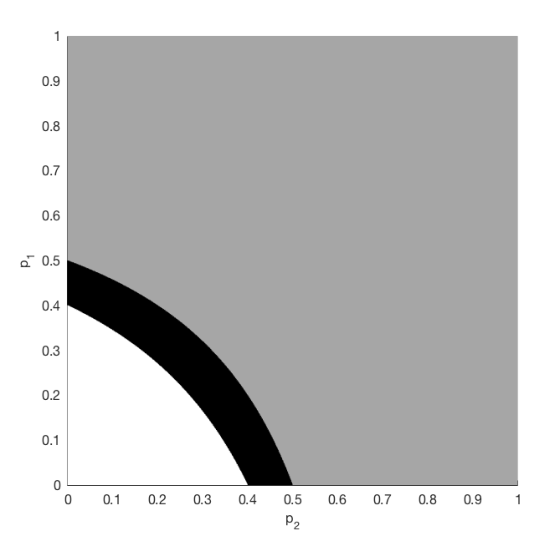
Refer to caption
(a) d=3d=3
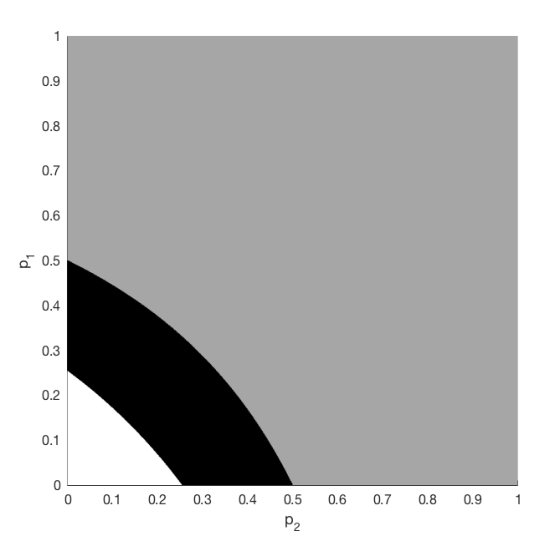
Refer to caption
(b) d=100d=100
Figure 1: The parameters (p1,p2)(p_{1},p_{2}) where Wp1⊗(ϑd∘Wp2)W_{p_{1}}\otimes(\vartheta_{d}\circ W_{p_{2}}) is positive and non-decomposable are in the interior of the black region. The gray region contains the remaining parameters where the map is positive.

In Fig. 1 we plot the parameter region where the linear map Wp1⊗(ϑd∘Wp2)W_{p_{1}}\otimes(\vartheta_{d}\circ W_{p_{2}}) is positive and non-decomposable in the cases d=3d=3 and d=100d=100.

6.2 Implications for the PPT squared conjecture

The PPT squared conjecture [3] asks for two completely positive and completely copositive maps T1,T2:ℳd→ℳdT_{1},T_{2}:\mathcal{M}_{d}\rightarrow\mathcal{M}_{d} whether their composition T2∘T1T_{2}\circ T_{1} is entanglement breaking. Here, PPT is short for “positive partial transposition” and linear maps that are both completely positive and completely copositive are often called PPT binding maps in the context of quantum information theory. It has been shown in [22] that this conjecture is equivalent to

Conjecture 6.1 (Equivalent formulation of PPT squared).

For any completely positive and completely copositive map T:ℳd1→ℳd2T:\mathcal{M}_{d_{1}}\rightarrow\mathcal{M}_{d_{2}} and any positive map P:ℳd2→ℳd3P:\mathcal{M}_{d_{2}}\rightarrow\mathcal{M}_{d_{3}} the composition P∘TP\circ T is decomposable.

Here we will prove:

Theorem 6.3.

If there exists a non-trivial tensor-stable positive map, then Conjecture 6.1 is false.

Proof.

Let P:ℳd1→ℳd2P:\mathcal{M}_{d_{1}}\rightarrow\mathcal{M}_{d_{2}} be a non-trivial tensor-stable positive map. We can assume without loss of generality that PP is not decomposable. Otherwise, Theorem 1.1 implies that for some n∈ℕn\in\mathbbm{N} the map P⊗nP^{\otimes n} is not decomposable, but tensor-stable positive, and we could consider it instead of PP.

Since PP is not decomposable, there exists a completely positive and completely copositive map T:ℳd2→ℳd1T:\mathcal{M}_{d_{2}}\rightarrow\mathcal{M}_{d_{1}} such that P∘TP\circ T is not completely positive. Let D:ℳ2→ℳ2D:\mathcal{M}_{2}\rightarrow\mathcal{M}_{2} be given by

D⁡(X)=⟨0​|X⁡|0⟩​|0⟩​⟨0|+⟨1|​X|1⟩|​1⟩​⟨1|,D(X)=\langle 0|X|0\rangle|0\rangle\!\langle 0|+\langle 1|X|1\rangle|1\rangle\!\langle 1|,

for any X∈ℳ2X\in\mathcal{M}_{2}, and note that this map is entanglement breaking [8]. Now consider the modified maps P~:ℳd1⊗ℳ2→ℳd2⊗ℳ2\tilde{P}:\mathcal{M}_{d_{1}}\otimes\mathcal{M}_{2}\rightarrow\mathcal{M}_{d_{2}}\otimes\mathcal{M}_{2} given by P~=P⊗D\tilde{P}=P\otimes D and T~:ℳd2→ℳd1⊗ℳ2\tilde{T}:\mathcal{M}_{d_{2}}\rightarrow\mathcal{M}_{d_{1}}\otimes\mathcal{M}_{2} given by

T~=T⊗|0⟩​⟨0|+T∘ϑd1⊗|1⟩​⟨1|.\displaystyle\tilde{T}=T\otimes|0\rangle\!\langle 0|+T\circ\vartheta_{d_{1}}\otimes|1\rangle\!\langle 1|.

Note that T~\tilde{T} is still completely positive and completely copositive. The map P~\tilde{P} is still tensor-stable positive, since by permuting subsystems we have P~⊗n≃P⊗n⊗D⊗n\tilde{P}^{\otimes n}\simeq P^{\otimes n}\otimes D^{\otimes n} which is positive since P⊗nP^{\otimes n} is positive and D⊗nD^{\otimes n} is entanglement breaking. Furthermore, observe that

P~∘T~=P∘T⊗|0⟩​⟨0|+P∘T∘ϑd1⊗|1⟩​⟨1|\tilde{P}\circ\tilde{T}=P\circ T\otimes|0\rangle\!\langle 0|+P\circ T\circ\vartheta_{d_{1}}\otimes|1\rangle\!\langle 1|

is neither completely positive nor completely co-positive, since P∘TP\circ T is not completely positive. Therefore, we can use Theorem 1.1 to find an n∈ℕn\in\mathbbm{N} such that (P~∘T~)⊗n=P~⊗n∘T~⊗n(\tilde{P}\circ\tilde{T})^{\otimes n}=\tilde{P}^{\otimes n}\circ\tilde{T}^{\otimes n} is not decomposable. But then T~⊗n\tilde{T}^{\otimes n} and P~⊗n\tilde{P}^{\otimes n} provide a counterexample for Conjecture 6.1. ∎

7 Conclusion and open problems

We have shown that a tensor-stable decomposable map has to be either completely positive or completely copositive. Moreover, we have derived bounds on the number of tensor powers a given linear map can stay decomposable for, if it does not belong to these two classes. Finally, we applied our results to construct non-decomposable positive maps, and to find a link between the existence problem of tensor-stable positive maps and the PPT squared conjecture in quantum information theory.

It would be interesting for future research to improve the quantitative bound from Theorem 1.2 and possibly to find optimal bounds on the decomposability of tensor powers of positive maps. For the mixed tensor powers of Werner maps, studied throughout our article, this could be possible by studying the set of quantum states with positive partial transpose introduced in Section 4.1.

Finally, it should also be noted that the results from Section 3 can be applied to similar questions for other mapping cones (as in Definition 2.1): Given a mapping cone 𝒞\mathcal{C} which elements P∈𝒞P\in\mathcal{C} satisfy P⊗n∈𝒞P^{\otimes n}\in\mathcal{C} for all n∈ℕn\in\mathbbm{N}? A mapping cone might contain the trivial examples of completely positive or completely copositive maps, but finding any example not belonging to these classes would also be an example of a non-trivial tensor-stable positive map (since mapping cones are always subcones of positive maps). Following the lines of the second proof of our Theorem 1.1 from Section 5 one could try to show that there are no such maps (except possibly the trivial ones) in a given mapping cone. To do this one would need to understand the properties of the linear maps leaving invariant the Choi matrices of the mapping cone in question. We will study this further in future works.

Acknowledgments

We would like to thank Chris Perry for proofreading this manuscript. We acknowledge financial support from the European Research Council (ERC Grant Agreement no 337603), the Danish Council for Independent Research (Sapere Aude) and VILLUM FONDEN via the QMATH Centre of Excellence (Grant No. 10059).

Appendix A Proof of Lemma 4.1

Lemma 4.1 has been shown originally in [16]. We include here a proof of this result to make the presentation selfcontained. Let 𝒞d\mathcal{C}_{d} denote the set from (22). Using the condition ∑i,j=12Qi​j=1\sum^{2}_{i,j=1}Q_{ij}=1 we can write each Q∈𝒞dQ\in\mathcal{C}_{d} as

Q=(xy1−x−y−zz).Q=\begin{pmatrix}x&y\\ 1-x-y-z&z\end{pmatrix}.

with parameters x,y,z∈ℝx,y,z\in\mathbbm{R}. With these parameters, the conditions that Q​Vd1QV^{1}_{d} and QT​Vd1Q^{T}V^{1}_{d} are entrywise positive, are equivalent to the set of inequalities

x−y\displaystyle x-y ≥0,\displaystyle\geq 0, (36)
x+αd​y\displaystyle x+\alpha_{d}y ≥0,\displaystyle\geq 0, (37)
y−z\displaystyle y-z ≥0,\displaystyle\geq 0, (38)
y+αd​z\displaystyle y+\alpha_{d}z ≥0,\displaystyle\geq 0, (39)
1−x−y−2​z\displaystyle 1-x-y-2z ≥0,\displaystyle\geq 0, (40)
1−x−y+(αd−1)​z\displaystyle 1-x-y+(\alpha_{d}-1)z ≥0,\displaystyle\geq 0, (41)
2​x+y+z\displaystyle 2x+y+z ≥1,\displaystyle\geq 1, (42)
−(αd−1)​x−αd​(y+z)\displaystyle-(\alpha_{d}-1)x-\alpha_{d}(y+z) ≥−αd.\displaystyle\geq-\alpha_{d}. (43)

Here, αd=d+1d−1\alpha_{d}=\frac{d+1}{d-1} and in particular we have αd>1\alpha_{d}>1 for any d∈ℕd\in\mathbbm{N}. Let 𝒞d′\mathcal{C}^{\prime}_{d} denote the set of all (x,y,z)∈ℝ3(x,y,z)\in\mathbbm{R}^{3} satisfying the above set of inequalities. Clearly, to prove Lemma 4.1 it is enough to show that the extreme points of 𝒞d′\mathcal{C}^{\prime}_{d} are given by

Q1′\displaystyle Q^{\prime}_{1} =12​(d+2)​(d+1,d+1,−(d−1)),\displaystyle=\frac{1}{2(d+2)}(d+1,d+1,-(d-1)),
Q2′\displaystyle Q^{\prime}_{2} =(1,0,0),\displaystyle=(1,0,0),
Q3′\displaystyle Q^{\prime}_{3} =14​(1,1,1),\displaystyle=\frac{1}{4}(1,1,1),
Q4′\displaystyle Q^{\prime}_{4} =12​(1,0,0),\displaystyle=\frac{1}{2}(1,0,0),
Q5′\displaystyle Q^{\prime}_{5} =12​(1,1,0).\displaystyle=\frac{1}{2}(1,1,0).

We will show this in the following two lemmas:

Lemma A.1.

The points Q1′,Q2′,Q3′,Q4′Q^{\prime}_{1},Q^{\prime}_{2},Q^{\prime}_{3},Q^{\prime}_{4}, and Q5′Q^{\prime}_{5} defined above are extreme points of 𝒞d′\mathcal{C}^{\prime}_{d}.

Proof.

Consider first (x,y,z)∈𝒞d′(x,y,z)\in\mathcal{C}^{\prime}_{d} satisfying x=yx=y. Using (41) and (39) we find that

1+(3​αd−1)​z=(1−2​x+(αd−1)​z)+2​(x+αd​z)≥01+(3\alpha_{d}-1)z=(1-2x+(\alpha_{d}-1)z)+2(x+\alpha_{d}z)\geq 0

showing that

z≥−13​αd−1=−d−12​(d+2).z\geq-\frac{1}{3\alpha_{d}-1}=-\frac{d-1}{2(d+2)}. (44)

From (38) and (42) we have that

x≥14.x\geq\frac{1}{4}. (45)

Finally, assuming z≥0z\geq 0 and using (40) or assuming z<0z<0 and using (41) implies that

x≤12.x\leq\frac{1}{2}. (46)

Now we can show that the points Q1,…,Q5Q_{1},\ldots,Q_{5} are indeed extreme points of the set 𝒞d′\mathcal{C}^{\prime}_{d}.

  • •

    Assume that there are (x1,y1,z1),(x2,y2,z2)∈𝒞d′(x_{1},y_{1},z_{1}),(x_{2},y_{2},z_{2})\in\mathcal{C}^{\prime}_{d} such that

    Q1′=p⁡(x1,y1,z1)+(1−p)​(x2,y2,z2)Q^{\prime}_{1}=p(x_{1},y_{1},z_{1})+(1-p)(x_{2},y_{2},z_{2})

    for some p∈(0,1)p\in\left(0,1\right). Since the first two entries of Q1′Q^{\prime}_{1} are equal we find

    p⁡(x1−y1)+(1−p)​(x2−y2)=0,p(x_{1}-y_{1})+(1-p)(x_{2}-y_{2})=0,

    which using (36) implies that x1=y1x_{1}=y_{1} and x2=y2x_{2}=y_{2}. Clearly, (44) implies that z1=z2=−d−12​(d+2)z_{1}=z_{2}=-\frac{d-1}{2(d+2)}. Inserting these in (42) and using that x1=y1x_{1}=y_{1} and x2=y2x_{2}=y_{2} shows that x1=y1=x2=y2=d+12​(d+2)x_{1}=y_{1}=x_{2}=y_{2}=\frac{d+1}{2(d+2)}, and thus Q1′Q^{\prime}_{1} is an extreme point of 𝒞d′\mathcal{C}^{\prime}_{d}.

  • •

    If for (x1,y1,z1),(x2,y2,z2)∈𝒞d′(x_{1},y_{1},z_{1}),(x_{2},y_{2},z_{2})\in\mathcal{C}^{\prime}_{d} we have

    Q3′=p⁡(x1,y1,z1)+(1−p)​(x2,y2,z2)Q^{\prime}_{3}=p(x_{1},y_{1},z_{1})+(1-p)(x_{2},y_{2},z_{2})

    for some p∈(0,1)p\in\left(0,1\right), then we can argue as for Q1′Q^{\prime}_{1} to conclude that x1=y1x_{1}=y_{1} and x2=y2x_{2}=y_{2}. Now, (45) implies that x1=x2=y1=y2=14x_{1}=x_{2}=y_{1}=y_{2}=\frac{1}{4}. Then, by (40) we find that x3=y3=14x_{3}=y_{3}=\frac{1}{4} as well, and Q3′Q^{\prime}_{3} is indeed an extreme point of 𝒞d′\mathcal{C}^{\prime}_{d}.

  • •

    If for (x1,y1,z1),(x2,y2,z2)∈𝒞d′(x_{1},y_{1},z_{1}),(x_{2},y_{2},z_{2})\in\mathcal{C}^{\prime}_{d} we have

    Q5′=p⁡(x1,y1,z1)+(1−p)​(x2,y2,z2)Q^{\prime}_{5}=p(x_{1},y_{1},z_{1})+(1-p)(x_{2},y_{2},z_{2})

    for some p∈(0,1)p\in\left(0,1\right), then we can argue as for Q1′Q^{\prime}_{1} to conclude that x1=y1x_{1}=y_{1} and x2=y2x_{2}=y_{2}. Now, (46) implies that x1=x2=y1=y2=12x_{1}=x_{2}=y_{1}=y_{2}=\frac{1}{2}, and using (40) and (41) we find that z1=z2=0z_{1}=z_{2}=0. Therefore, Q5′Q^{\prime}_{5} is also an extreme point of 𝒞d′\mathcal{C}^{\prime}_{d}.

  • •

    Let (x1,y1,z1),(x2,y2,z2)∈𝒞d′(x_{1},y_{1},z_{1}),(x_{2},y_{2},z_{2})\in\mathcal{C}^{\prime}_{d} be such that

    Q4′=p⁡(x1,y1,z1)+(1−p)​(x2,y2,z2)Q^{\prime}_{4}=p(x_{1},y_{1},z_{1})+(1-p)(x_{2},y_{2},z_{2})

    for some p∈(0,1)p\in\left(0,1\right). Since the last two entries of Q4′Q^{\prime}_{4} are equal we find

    p⁡(y1−z1)+(1−p)​(y2−z2)=0,p(y_{1}-z_{1})+(1-p)(y_{2}-z_{2})=0,

    which using (38) implies that y1=z1y_{1}=z_{1} and y2=z2y_{2}=z_{2}. By (39) and since the last two entries of Q4′Q^{\prime}_{4} vanish we need to have y1=z1=y2=z2=0y_{1}=z_{1}=y_{2}=z_{2}=0. Using (42) we find that x1=x2=12x_{1}=x_{2}=\frac{1}{2}, which shows that Q4′Q^{\prime}_{4} is an extreme point of 𝒞d′\mathcal{C}^{\prime}_{d}.

  • •

    To prove extremality of Q2′Q^{\prime}_{2} one more observations. First, note that if for (x,y,z)∈𝒞d′(x,y,z)\in\mathcal{C}^{\prime}_{d} we would have x>1x>1, then by (40) and (38) we have z<0z<0. Then, (39) implies that y>0y>0, which leads to a contradiction in (41). Therefore, we have

    x≤1.x\leq 1. (47)

    Finally, let (x1,y1,z1),(x2,y2,z2)∈𝒞d′(x_{1},y_{1},z_{1}),(x_{2},y_{2},z_{2})\in\mathcal{C}^{\prime}_{d} such that

    Q2′=p⁡(x1,y1,z1)+(1−p)​(x2,y2,z2)Q^{\prime}_{2}=p(x_{1},y_{1},z_{1})+(1-p)(x_{2},y_{2},z_{2})

    for some p∈(0,1)p\in\left(0,1\right). Then, by (47) we have x1=x2=1x_{1}=x_{2}=1. Arguing as for Q4′Q^{\prime}_{4} (using that the final two entries of Q2′Q^{\prime}_{2} coincide) we also have y1=z1y_{1}=z_{1} and y2=z2y_{2}=z_{2}. Now, (39) and (40) show that y1=z1=y2=z2=0y_{1}=z_{1}=y_{2}=z_{2}=0 proving that Q2′Q^{\prime}_{2} is an extreme point of 𝒞d′\mathcal{C}^{\prime}_{d}.

∎

We still need to show the following:

Lemma A.2.

The points Q1′,Q2′,Q3′,Q4′,Q5′Q^{\prime}_{1},Q^{\prime}_{2},Q^{\prime}_{3},Q^{\prime}_{4},Q^{\prime}_{5} are all the extreme points of 𝒞d′\mathcal{C}^{\prime}_{d}.

Proof.

For this consider the plane

𝒮:={(x,y,z)∈ℝ3:y=12​(1−x−z)}.\mathcal{S}:=\{(x,y,z)\in\mathbbm{R}^{3}~:~y=\frac{1}{2}(1-x-z)\}. (48)

Inserting y=12​(1−x−z)y=\frac{1}{2}(1-x-z) into the inequalities (36),(37),…,(43) leads to the set of inequalities

3​x+z\displaystyle 3x+z ≥1,\displaystyle\geq 1, (49)
x+3​z\displaystyle x+3z ≤1,\displaystyle\leq 1, (50)
(2−αd)​x−αd​z\displaystyle(2-\alpha_{d})x-\alpha_{d}z ≥−αd.\displaystyle\geq-\alpha_{d}. (51)
−x+(2​αd−1)​z\displaystyle-x+(2\alpha_{d}-1)z ≥−1.\displaystyle\geq-1. (52)

characterizing the x,z∈ℝx,z\in\mathbbm{R} such that (x,12​(1−x−z),z)∈𝒮∩𝒞d′(x,\frac{1}{2}(1-x-z),z)\in\mathcal{S}\cap\mathcal{C}_{d}^{\prime}. By computing the intersection points of the lines given by the equality cases of the inequalities (49),(50) and (52) it is easy to see that the extreme points 𝒮∩𝒞d′\mathcal{S}\cap\mathcal{C}_{d}^{\prime} are Q1′,Q2′Q^{\prime}_{1},Q^{\prime}_{2} and Q3′Q^{\prime}_{3}. Note, that (51) turns out to be redundant for the definition of this convex set. See Fig. 2 for a picture of how 𝒮\mathcal{S} intersects the set 𝒞d′\mathcal{C}_{d}^{\prime}.

Refer to caption
Figure 2: The set 𝒞5′\mathcal{C}^{\prime}_{5} together with the intersecting plane 𝒮\mathcal{S}.

Let (x,y,z)∈𝒞d′∖({Q5′,Q4′}∪𝒮)(x,y,z)\in\mathcal{C}^{\prime}_{d}\setminus(\{Q^{\prime}_{5},Q^{\prime}_{4}\}\cup\mathcal{S}) and assume first that y>12​(1−x−z)y>\frac{1}{2}(1-x-z). Now, consider

λ:=4​(y−12​(1−x−z))>0.\lambda:=4\left(y-\frac{1}{2}\left(1-x-z\right)\right)>0.

We will show that λ<1\lambda<1 and that

(x′,y′,z′)=11−λ​((x,y,z)−λ​Q5′)∈𝒮∩𝒞d′,(x^{\prime},y^{\prime},z^{\prime})=\frac{1}{1-\lambda}\left((x,y,z)-\lambda Q^{\prime}_{5}\right)\in\mathcal{S}\cap\mathcal{C}^{\prime}_{d}, (53)

showing that (x,y,z)(x,y,z) is not an extreme point of 𝒞d′\mathcal{C}^{\prime}_{d}. Note that by (40),(41), and (36) we have that

x+2​y+z=d+22​d​(x+y+2​z)+d−1d​(x+y−(αd−1)​z)+12​(y−x)≤32.x+2y+z=\frac{d+2}{2d}\left(x+y+2z\right)+\frac{d-1}{d}\left(x+y-(\alpha_{d}-1)z\right)+\frac{1}{2}\left(y-x\right)\leq\frac{3}{2}. (54)

We have equality in (54) iff we have equality in (40),(41), and (36). This is equivalent to (x,y,z)=Q5′(x,y,z)=Q^{\prime}_{5}, which we excluded previously. Therefore, our point (x,y,z)(x,y,z) satisfies (54) strictly, which is easily seen to be equivalent to λ<1\lambda<1. Finally, it is easy to verify that (x′,y′,z′)(x^{\prime},y^{\prime},z^{\prime}) defined in (53) satisfies the inequalities (49),(50),(51), and (52) showing that (x′,y′,z′)∈𝒮∩𝒞d′(x^{\prime},y^{\prime},z^{\prime})\in\mathcal{S}\cap\mathcal{C}^{\prime}_{d}.

Now, let (x,y,z)∈𝒞d′∖({Q5′,Q4′}∪𝒮)(x,y,z)\in\mathcal{C}^{\prime}_{d}\setminus(\{Q^{\prime}_{5},Q^{\prime}_{4}\}\cup\mathcal{S}) with y<12​(1−x−z)y<\frac{1}{2}(1-x-z). Similarly to the previous argument we consider

λ:=−4​(y−12​(1−x−z))>0.\lambda:=-4\left(y-\frac{1}{2}\left(1-x-z\right)\right)>0.

Again, we will show that λ<1\lambda<1 and that

(x′,y′,z′)=11−λ​((x,y,z)−λ​Q2′)∈𝒮∩𝒞d′,(x^{\prime},y^{\prime},z^{\prime})=\frac{1}{1-\lambda}\left((x,y,z)-\lambda Q^{\prime}_{2}\right)\in\mathcal{S}\cap\mathcal{C}^{\prime}_{d}, (55)

showing that (x,y,z)(x,y,z) is not an extreme point of 𝒞d′\mathcal{C}^{\prime}_{d}. By (42),(37), and (38) we have that

x+2​y+z=12​(2​x+y+z)+2​(d−1)d​(y+αd​z)+d+2d​(y−z)≥12.x+2y+z=\frac{1}{2}\left(2x+y+z\right)+\frac{2(d-1)}{d}\left(y+\alpha_{d}z\right)+\frac{d+2}{d}\left(y-z\right)\geq\frac{1}{2}. (56)

We have equality in (56) iff we have equality in (42),(37), and (38). This is equivalent to (x,y,z)=Q4′(x,y,z)=Q^{\prime}_{4}, which we excluded previously. Therefore, our point (x,y,z)(x,y,z) satisfies (56) strictly, which is easily seen to be equivalent to λ<1\lambda<1. Finally, it is easy to verify that (x′,y′,z′)(x^{\prime},y^{\prime},z^{\prime}) defined in (55) satisfies the inequalities (49),(50),(51), and (52) showing that (x′,y′,z′)∈𝒮∩𝒞d′(x^{\prime},y^{\prime},z^{\prime})\in\mathcal{S}\cap\mathcal{C}^{\prime}_{d}.

The above argument shows that there are no further extreme points (x,y,z)∈𝒞d′∖({Q5′,Q4′}∪𝒮)(x,y,z)\in\mathcal{C}^{\prime}_{d}\setminus(\{Q^{\prime}_{5},Q^{\prime}_{4}\}\cup\mathcal{S}) of the set 𝒞d′\mathcal{C}^{\prime}_{d}. Indeed, Q1′,…,Q5′Q^{\prime}_{1},\ldots,Q^{\prime}_{5} are all the extreme points of 𝒞d′\mathcal{C}^{\prime}_{d} finishing the proof. ∎

References

  • [1] A. Müller-Hermes, D. Reeb, and M. M. Wolf, “Positivity of linear maps under tensor powers,” Journal of Mathematical Physics, vol. 57, no. 1, p. 015202, 2016.
  • [2] S. N. Filippov and K. Y. Magadov, “Positive tensor products of maps and n-tensor-stable positive qubit maps,” Journal of Physics A: Mathematical and Theoretical, vol. 50, no. 5, p. 055301, 2017.
  • [3] M. Christandl, “PPT square conjecture,” Banff International Research Station workshop: Operator structures in Quantum Information Theory, 2012.
  • [4] M.-D. Choi, “Completely positive linear maps on complex matrices,” Linear algebra and its applications, vol. 10, no. 3, pp. 285–290, 1975.
  • [5] A. Jamiołkowski, “Linear transformations which preserve trace and positive semidefiniteness of operators,” Reports on Mathematical Physics, vol. 3, no. 4, pp. 275–278, 1972.
  • [6] E. Størmer, “Extension of positive maps into B⁡(H)B(H),” Journal of Functional Analysis, vol. 66, no. 2, pp. 235–254, 1986.
  • [7] Ł. Skowronek, E. Størmer, and K. Życzkowski, “Cones of positive maps and their duality relations,” Journal of Mathematical Physics, vol. 50, no. 6, p. 062106, 2009.
  • [8] M. Horodecki, P. W. Shor, and M. B. Ruskai, “Entanglement breaking channels,” Reviews in Mathematical Physics, vol. 15, no. 06, pp. 629–641, 2003.
  • [9] S. L. Woronowicz, “Positive maps of low dimensional matrix algebras,” Reports on Mathematical Physics, vol. 10, no. 2, pp. 165–183, 1976.
  • [10] E. Størmer, “Decomposable positive maps on C⋆C^{\star}-algebras,” Proceedings of the American Mathematical Society, vol. 86, no. 3, pp. 402–404, 1982.
  • [11] S. Boyd and L. Vandenberghe, Convex optimization. Cambridge university press, 2004.
  • [12] R. F. Werner, “Quantum states with Einstein-Podolsky-Rosen correlations admitting a hidden-variable model,” Physical Review A, vol. 40, no. 8, p. 4277, 1989.
  • [13] R. F. Werner and A. S. Holevo, “Counterexample to an additivity conjecture for output purity of quantum channels,” Journal of Mathematical Physics, vol. 43, no. 9, pp. 4353–4357, 2002.
  • [14] M. Horodecki and P. Horodecki, “Reduction criterion of separability and limits for a class of distillation protocols,” Physical Review A, vol. 59, no. 6, p. 4206, 1999.
  • [15] R. Penrose, “A generalized inverse for matrices,” in Mathematical proceedings of the Cambridge philosophical society, vol. 51, no. 3. Cambridge University Press, 1955, pp. 406–413.
  • [16] K. G. H. Vollbrecht and M. M. Wolf, “Activating distillation with an infinitesimal amount of bound entanglement,” Physical review letters, vol. 88, no. 24, p. 247901, 2002.
  • [17] D. Chruściński and A. Kossakowski, “Multipartite invariant states. I. Unitary symmetry,” Physical Review A, vol. 73, no. 6, p. 062314, 2006.
  • [18] ——, “Quantum entanglement and symmetry,” in Journal of Physics: Conference Series, vol. 87, no. 1. IOP Publishing, 2007, p. 012008.
  • [19] K. Audenaert, J. Eisert, E. Jané, M. Plenio, S. Virmani, and B. De Moor, “Asymptotic relative entropy of entanglement,” Physical review letters, vol. 87, no. 21, p. 217902, 2001.
  • [20] T. Eggeling, K. G. H. Vollbrecht, R. F. Werner, and M. M. Wolf, “Distillability via protocols respecting the positivity of partial transpose,” Physical review letters, vol. 87, no. 25, p. 257902, 2001.
  • [21] L. Lami and M. Huber, “Bipartite depolarizing maps,” Journal of Mathematical Physics, vol. 57, no. 9, p. 092201, 2016.
  • [22] M. Christandl, A. Müller-Hermes, and M. M. Wolf, “When do composed maps become entanglement breaking?” arXiv preprint arXiv:1807.01266, 2018.