跳到论文正文
W Papers独立论文阅读器 arXiv:1805.11484 论文正文 计算阅读时间 · 0%
引用这篇论文根据当前论文元数据生成,正式投稿前建议核对。


License: arXiv.org perpetual non-exclusive license
arXiv:1805.11484v1 [math.NA] 29 May 2018

A Bloch transform based numerical method for the rough surface scattering problems

Ruming Zhang ††thanks: Center for Industrial Mathematics, University of Bremen; rzhang@uni-bremen.de
Abstract

In this paper, we will study the Bloch transformed rough surface scattering problems, and propose a numerical method based on the Bloch transformed problems. Based on the mathematical theory of the scattering problems from locally perturbed periodic surfaces, the same techniques will be applied to the rough surface scattering problems, and an equivalent coupled family of quasi-periodic scattering problems in one periodic cell will be established. The most important result obtained in this paper is on the finite Fourier series approximation of the Bloch transformed field with respect to the quasi-periodicity parameter. It will be proved that the finite series is exactly the Bloch transformed solution corresponds to truncated rough surfaces. Thus the truncation provides a reasonable approximation, and could be applied to the numerical solutions. Based on the approximation, a numerical method is proposed for the rough surface scattering problems. The convergence of the numerical method is proved and illustrated by the numerical experiments. The method provides a completely new perspective for the rough surface scattering problems. There is possibility that some high order method will be developed based on this new method.

1 Introduction

The scattering problems from rough structures are always interesting but challenging topics. Mathematicians have been working on both the theoretical analysis and numerical implementation of this topic for decades. Based on integral equations, the well-posedness of the problems has been investigated, see [CWR96, CWZ98, CWRZ99, ZCW03]. A Nyström method for the integral equation on the real line has been developed for the rough surface scattering problems, see [MACK00, AHC02]. In 2005, Chandler-Wilde and Monk proposed a variational method (see [CM05]) for the investigation of the well-posedness of the scattering problems from rough surfaces in both 2D and 3D spaces. Based on the variational method, the unique solvability of the scattering from rough surfaces has been proved in weighted Sobolev spaces in [CE10], in which more generalized cases (e.g. plane waves in 2D spaces) are included. Similar results in weighted Sobolev spaces has been shown for more generalized boundary conditions in [HLQZ15]. Based on the variational formulation in weighted spaces, a so-called ”finite section method” has been proposed for numerical approximations in [CE10].

Recently, a Floquet-Bloch transform based method has been proposed to treat scattering problems from a special kind of rough surfaces, i.e., the locally perturbed periodic surfaces. To the author’s knowledge, this method was first introduced in the paper [Coa12], for scattering problems from locally perturbed periodic mediums. For the non-periodic incident fields (e.g., the Herglotz wave functions or the point sources) scattered by locally perturbed periodic surfaces, the scattering problems are transformed into an equivalent coupled family of quasi-periodic scattering problems by the Bloch transform (see [LN15, Lec17]). Based on the theoretical analysis for the Bloch-transformed scattering problems, convergent numerical methods have been developed for the scattering problems, for periodic surfaces see [LZ17a], and for locally perturbed periodic surfaces see [LZ17b]. Discussions are also made for 3D acoustic and electromagnetic problems, and the first numerical experiment has been carried out for the 3D Helmholtz equations, see [LZ17c]. For the scattering problems from locally perturbed periodic layers, similar method has been adopted in [HN15]. The Bloch transform was also applied to the scattering problems in locally perturbed periodic waveguides, see [FJ15].

In this paper, the Floquet-Bloch transform will be applied to the rough surface scattering problems. With the technique introduced in [Lec17], the problem is transformed into one defined in an infinite rectangle. With the help of the Bloch transform, the new problem is decomposed into a coupled family of quasi-periodic scattering problems, and the equivalence between the original problem and the coupled family of quasi-periodic problems will be proved. The main difficulty comes from the term involves the perturbation, which is no longer compactly supported, as that for locally perturbed cases. An interesting result shows that, the approximated finite Fourier series of the Bloch transformed field with respect to the quasi-periodicity parameter is exactly the Bloch transformed solution of the scattering problem with truncated rough surface. It could be a good choice of approximation for the scattering problems in unbounded domains, for the numerical method of the locally perturbed problems have been well studied in [LZ17b], and a high order method was developed in [Zha18]. Based on this result, a finite element method will be developed for the numerical solution. Although there are convergent numerical methods for the simulation of the scattering problems, e.g., the one based on the integral equations (see [AHC02, MACK00]) or variational formulations (see [CE10]), the new method may provide very different perspective for the rough surface scattering problems. It is also expected that the Bloch transform based numerical method will be improved and a high order method will be developed following [Zha18] in the future.

The rest of the paper is organized as follows. In Section 2, we will recall the mathematical model of the rough surface scattering problems and its unique solvability. In Section 3, we will formulate the weak formulation of the Bloch transformed scattering problems, and study the equivalence and unique solvability of the newly established variational problem. In Section 4, the finite Fourier series approximation of the Bloch transformed fields will be studied. Based on the approximation, a finite element method will be proposed in Section 5, and details of the numerical implementation will be explained in Section 6. In the last section, we will give several numerical experiments to illustrate the convergence result obtained in Section 5

2 Scattering from rough surfaces

In this section, we recall the mathematical modal and well-posedness of the scattering problems from rough surfaces in two dimensional spaces. For details we refer to the papers [CM05, CE10].

Let ζ\zeta be a bounded function defined in ℝ\mathbb{R}. In this paper, we have to require that the following assumption holds for the functions ζ\zeta.

Assumption 1.

ζ\zeta is a Lipschitz continuous function defined on ℝ\mathbb{R}. Suppose there is a positive C>0C>0 such that

‖ζ‖1,∞≤C.\left\|\zeta\right\|_{1,\infty}\leq C.

Without loss of generality, assume that ζ⁡(t)≥c>0\zeta(t)\geq c>0 for any t∈ℝt\in\mathbb{R}.

Refer to caption
Figure 1: A global rough surface.

Define the rough surface by

Γ:={(x1,ζ⁡(x1)):x1∈ℝ}.\Gamma:=\left\{(x_{1},\zeta(x_{1})):\,x_{1}\in\mathbb{R}\right\}.

Let Γh\Gamma_{h} be defined by the straight line ℝ×{h}\mathbb{R}\times\{h\} for any h∈ℝh\in\mathbb{R}. Suppose HH is a constant satisfies H>max⁡{‖ζ‖∞}H>\max\left\{\|\zeta\|_{\infty}\right\}, then ΓH\Gamma_{H} is a straight line lies above Γ\Gamma. Define the domains by

Ω:={(x1,x2):x2>ζ⁡(x1)},ΩH:={(x1,x2):ζ⁡(x1)<x2<H}.\Omega:=\left\{(x_{1},x_{2}):\,x_{2}>\zeta(x_{1})\right\},\quad\Omega_{H}:=\left\{(x_{1},x_{2}):\,\zeta(x_{1})<x_{2}<H\right\}.

Given an incident field uiu^{i} that satisfies the Helmholtz equation

Δ​ui+k2​ui=0​ in ​Ω,\Delta u^{i}+k^{2}u^{i}=0\text{ in }\Omega,

it is scattered by the impenetrable surface Γ\Gamma. Then the total field uu satisfies the Helmholtz equation in Ω\Omega as well, i.e.,

Δ​u+k2​u=0​ in ​Ω.\Delta u+k^{2}u=0\text{ in }\Omega. (1)

Assume that the total field uu also satisfies the homogeneous Dirichlet boundary condition on the boundary Γ\Gamma, i.e.,

u=0​ on ​Γ.u=0\text{ on }\Gamma. (2)
Remark 2.

In this paper, only the Dirichlet boundary condition is considered. However, it is possible to treat problems with different conditions, such as the impedance boundary condition (see [Lec17]) or inhomogeneous mediums.

The scattered field us:=u−uiu^{s}:=u-u^{i} satisfies the so-called angular spectrum representation as a radiation condition (see [CM05]), i.e.,

us​(x1,x2)=12​π​∫ℝei​x1⋅ξ+i​k2−|ξ|2​(x2−H)​us^​(ξ,H)​𝑑ξ,x2≥H,u^{s}(x_{1},x_{2})=\frac{1}{2\pi}\int_{\mathbb{R}}e^{\mathrm{i}x_{1}\cdot{\xi}+\mathrm{i}\sqrt{k^{2}-|{\xi}|^{2}}(x_{2}-H)}\widehat{u^{s}}({\xi},H)\,\mathrm{d}\xi\,,\quad x_{2}\geq H, (3)

where u^s\widehat{u}^{s} is the Fourier transform of usu^{s} on ΓH\Gamma_{H}, and k2−|ξ|2=i​|ξ|2−k2\sqrt{k^{2}-|{\xi}|^{2}}=\mathrm{i}\sqrt{|\xi|^{2}-k^{2}} when |ξ|>k|\xi|>k. The radiation condition (3) is equivalent to the following boundary condition

∂us∂x2​(x1,H)=T+​[us|ΓH], on ​ΓH,\frac{\partial u^{s}}{\partial x_{2}}(x_{1},H)=T^{+}\left[u^{s}\big|_{\Gamma_{H}}\right],\quad\text{ on }\Gamma_{H},

where T+T^{+} is the Dirichlet-to-Neumann map defined by

T+​φ=i2​π​∫ℝk2−|ξ|s​ei​x1⋅ξ​φ^​(ξ)​𝑑ξ for ​φ=12​π​∫ℝei​x1⋅ξ​φ^​(ξ)​𝑑ξ.T^{+}\varphi=\frac{\mathrm{i}}{{2\pi}}\int_{\mathbb{R}}\sqrt{k^{2}-|{\xi}|^{s}}e^{\mathrm{i}x_{1}\cdot{\xi}}\widehat{\varphi}({\xi})\,\mathrm{d}\xi\,\quad\text{ for }\varphi=\frac{1}{2\pi}\int_{\mathbb{R}}e^{\mathrm{i}x_{1}\cdot{\xi}}\widehat{\varphi}({\xi})\,\mathrm{d}\xi\,. (4)

T+T^{+} is a continuous operator from Hr1/2​(ΓH)H_{r}^{1/2}(\Gamma_{H}) into Hr−1/2(ΓH)H_{r}^{-1/2}(\Gamma_{H}) for any |r|<1|r|<1 (see [CE10]). Thus the total field satisfies the boundary condition on Γ\Gamma

∂u∂x2​(x1,H)=T+​[u|ΓH]+f, where ​f:=∂ui∂x2​(x1,H)−T+​[ui|ΓH].\frac{\partial u}{\partial x_{2}}(x_{1},H)=T^{+}\left[u\big|_{\Gamma_{H}}\right]+f,\quad\text{ where }f:=\frac{\partial u^{i}}{\partial x_{2}}(x_{1},H)-T^{+}\left[u^{i}|_{\Gamma_{H}}\right]. (5)

The scattering problem is now turned into a problem that defined on the domain ΩH\Omega_{H} with a finite height. The weak formulation for the scattering problem is, given any f∈H−1/2(ΓH)f\in H^{-1/2}(\Gamma_{H}), to find a solution u∈H~1​(ΩH)u\in\widetilde{H}^{1}(\Omega_{H}) such that

∫ΩH[∇u⋅∇v¯−k2​u​v¯]​𝑑x−∫ΓHT+​[u|ΓH]​v¯​𝑑s=∫ΓHf​v¯​𝑑s,\int_{\Omega_{H}}\left[\nabla u\cdot\nabla\overline{v}-k^{2}u\overline{v}\right]\,\mathrm{d}x\,-\int_{\Gamma_{H}}T^{+}\left[u|_{\Gamma_{H}}\right]\overline{v}\,\mathrm{d}s\,=\int_{\Gamma_{H}}f\overline{v}\,\mathrm{d}s\,, (6)

for all v∈H~1​(ΩH)v\in\widetilde{H}^{1}(\Omega_{H}) with compact support in ΩH¯\overline{\Omega_{H}}. The variational problem could also be analysed in the weighted Sobolev space H~r1​(ΩH)\widetilde{H}_{r}^{1}(\Omega_{H}).

Remark 3.

The tilde in H~r1​(ΩH)\widetilde{H}_{r}^{1}(\Omega_{H}) shows that the functions in this space belong to Hr1​(ΩH)H_{r}^{1}(\Omega_{H}) and satisfy homogeneous Dirichlet boundary condition on Γ\Gamma. Similar notations are utilized for other spaces, e.g., H0r​(WΛ∗,H~αs​(DHΛ))H_{0}^{r}({W_{\hskip-1.0pt{\Lambda}^{\ast}}};\widetilde{H}_{\alpha}^{s}(D^{\Lambda}_{H})).

From [CE10], the unique solubility of the variational problem 6 has been proved in weighted Sobolev spaces.

Theorem 4.

If Γ\Gamma is Lipschitz continuous, f∈Hr−1/2(ΓH)f\in H_{r}^{-1/2}(\Gamma_{H}) for |r|<1|r|<1, then there is a unique solution u∈H~r1​(ΩH)u\in\widetilde{H}_{r}^{1}(\Omega_{H}) for the variational problem (6).

3 The Bloch transform and the scattering problems

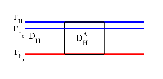
In this section, we apply the Bloch transform to the scattering problems. As the Bloch transform only works on functions defined in periodic domains, the first step is to transform the problem into one defined in a periodic domain, and then apply the Bloch transform to the new problem (see [Lec17, LZ17c]). In this paper, the procedure will be altered slightly, i.e., to transform the scattering problem into the new one defined in the infinite rectangle DH:=ℝ×[h0,H]D_{H}:=\mathbb{R}\times[h_{0},H] where 0<h0,‖ζ‖∞<H0<h_{0},\,\|\zeta\|_{\infty}<H. Let ΓHΛ\Gamma^{\Lambda}_{H} and DHΛD^{\Lambda}_{H} be ΓH\Gamma_{H} and DHD_{H} restricted in one periodic cell WΛ×ℝ{W_{\hskip-1.0pt{\Lambda}}}\times\mathbb{R}, i.e.,

ΓHΛ=ΓH∩[WΛ×ℝ],DHΛ=DH∩[WΛ×ℝ].\Gamma^{\Lambda}_{H}=\Gamma_{H}\cap\left[{W_{\hskip-1.0pt{\Lambda}}}\times\mathbb{R}\right],\quad D^{\Lambda}_{H}=D_{H}\cap\left[{W_{\hskip-1.0pt{\Lambda}}}\times\mathbb{R}\right].
Refer to caption
Figure 2: Strip DHD_{H} and one periodic cell DHΛD^{\Lambda}_{H}.

Let Θ\Theta be a diffeomorphism that maps ΩH0\Omega_{H_{0}} to DH0D_{H_{0}} for some ‖ζ‖∞<H0<H\|\zeta\|_{\infty}<H_{0}<H, and extend Θ\Theta by identity in ℝ×[H0,∞)\mathbb{R}\times[H_{0},\infty). Thus the support of Θ−I\Theta-I is contained in DH0D_{H_{0}}.

Remark 5.

With Assumption 1, we can always find a diffeomorphism Θ\Theta, such that Θ\Theta and Θ−1\Theta^{-1} are both Lipschitz continuous in ΩH\Omega_{H}. An example for the definition of Θ\Theta is

Θ:x↦(x1,x2+(H0−x2)3(H0−h0)3​(ζ⁡(x1)−h0)) when ​x∈DH0,\Theta:\,{x}\mapsto\left(x_{1},x_{2}+\frac{(H_{0}-x_{2})^{3}}{(H_{0}-h_{0})^{3}}\left(\zeta(x_{1})-h_{0}\right)\right)\quad\text{ when }x\in D_{H_{0}}, (7)

and then extend it by the identity operator II when x2≥H0x_{2}\geq H_{0}.

Let the transformed total field uT:=u∘Θu_{T}:=u\,\circ\,\Theta, then by direct calculation, uT∈H~r1​(DH)u_{T}\in\widetilde{H}_{r}^{1}(D_{H}) satisfies the following variational problem in the periodic domain DHD_{H}

∫DH[A∇uT⋅∇vT¯−k2cuTvT¯]dx−∫ΓHT+[uT|ΓH]vT¯ds=∫ΓHfvT¯ds,\int_{D_{H}}\left[A\nabla u_{T}\cdot\nabla\overline{v_{T}}-k^{2}cu_{T}\overline{v_{T}}\right]\,\mathrm{d}x\,-\int_{\Gamma_{H}}T^{+}\left[u_{T}|_{\Gamma_{H}}\right]\overline{v_{T}}\,\mathrm{d}s\,=\int_{\Gamma_{H}}f\overline{v_{T}}\,\mathrm{d}s\,, (8)

for all vT:=v∘Θ∈H~1​(DH)v_{T}:=v\circ\Theta\in\widetilde{H}^{1}(D_{H}),

AΘ​(x):=|det∇Θ​(x)|​[(∇Θ​(x))−1​(∇Θ​(x))−T]∈L∞​(ΩH,ℝ2×2),\displaystyle A_{\Theta}({x}):=\left|\det\nabla\Theta({x})\right|\left[\left(\nabla\Theta({x})\right)^{-1}\left(\nabla\Theta({x})\right)^{-T}\right]\in L^{\infty}\left(\Omega_{H},\mathbb{R}^{2\times 2}\right),
cΘ​(x):=|det∇Θ​(x)|∈L∞​(ΩH).\displaystyle c_{\Theta}({x}):=\left|\det\nabla\Theta({x})\right|\in L^{\infty}(\Omega_{H}).

Thus the support of both AΘA_{\Theta} and cΘc_{\Theta} are subsets of DH0D_{H_{0}}.

Remark 6.

From the definitions of AΘA_{\Theta} and cΘc_{\Theta}, if ζ\zeta has higher regularities, e.g., if ζ∈Cn,1​(ℝ)\zeta\in C^{n,1}(\mathbb{R}) for some positive integer n≥1n\geq 1, AΘA_{\Theta} and cΘc_{\Theta} will have higher regularities as well, i.e., AΘ∈Wn−1,∞​(ΩH,ℝ2×2)A_{\Theta}\in W^{n-1,\infty}(\Omega_{H},\mathbb{R}^{2\times 2}) and cΘ∈Wn−1,∞​(ΩH)c_{\Theta}\in W^{n-1,\infty}(\Omega_{H}). Moreover, there is a constant C>0C>0 depends only on ζ\zeta such that

‖AΘ‖Wn−1,∞​(ΩH,ℝ2×2),‖cΘ‖Wn−1,∞​(ΩH)≤C​‖ζ‖Wn,∞​(ℝ)\|A_{\Theta}\|_{W^{n-1,\infty}(\Omega_{H},\mathbb{R}^{2\times 2})},\,\|c_{\Theta}\|_{W^{n-1,\infty}(\Omega_{H})}\leq C\|\zeta\|_{W^{n,\infty}(\mathbb{R})} (9)

From direct calculations, we rewrite the variational problem (8) as

∫DH[∇uT⋅∇vT¯−k2​uT​vT¯]​dx−∫ΓHT+​[uT|ΓH]​vT¯​ds+∫DH[(AΘ−I)∇uT⋅∇vT¯−k2(cΘ−1)uTvT¯]dx=∫ΓHfvT¯ds.\begin{aligned} &\int_{D_{H}}\left[\nabla u_{T}\cdot\nabla\overline{v_{T}}-k^{2}u_{T}\overline{v_{T}}\right]\,\mathrm{d}x\,-\int_{\Gamma_{H}}T^{+}\left[u_{T}|_{\Gamma_{H}}\right]\overline{v_{T}}\,\mathrm{d}s\,\\ &\qquad+\int_{D_{H}}\left[(A_{\Theta}-I)\nabla u_{T}\cdot\nabla\overline{v_{T}}-k^{2}(c_{\Theta}-1)u_{T}\overline{v_{T}}\right]\,\mathrm{d}x\,=\int_{\Gamma_{H}}f\overline{v_{T}}\,\mathrm{d}s\,\end{aligned}.

Use the property of the Bloch transform, let wB=𝒥DH​uTw_{B}=\mathcal{J}_{D_{H}}u_{T}, vB=𝒥DH​v¯¯v_{B}=\overline{\mathcal{J}_{D_{H}}\overline{v}}, then wB∈H0r​(WΛ∗,H~α1​(DHΛ))w_{B}\in H_{0}^{r}({W_{\hskip-1.0pt{\Lambda}^{\ast}}};\widetilde{H}_{\alpha}^{1}(D^{\Lambda}_{H})), the variational form is equivalent to

∫WΛ∗aα(wB(α,⋅),vB(α,⋅))dα+∫DH[(AΘ−I)∇uT⋅∇v¯−k2(cΘ−1)uTv¯]dx=∫WΛ∗∫ΓHΛ[𝒥ΓH​f]​(α,x)​v⁡(α,x)¯​ds​(x)​dα,,\begin{aligned} \int_{W_{\hskip-1.0pt{\Lambda}^{\ast}}}a_{\alpha}(w_{B}({\alpha},\cdot),v_{B}({\alpha},\cdot))\,\mathrm{d}\alpha\,+\int_{D_{H}}\left[(A_{\Theta}-I)\nabla u_{T}\cdot\nabla\overline{v}-k^{2}(c_{\Theta}-1)u_{T}\overline{v}\right]\,\mathrm{d}x\,\\ =\int_{W_{\hskip-1.0pt{\Lambda}^{\ast}}}\int_{\Gamma^{\Lambda}_{H}}\left[\mathcal{J}_{\Gamma_{H}}f\right](\alpha,x)\overline{v(\alpha,x)}\,\mathrm{d}s(x)\,\,\mathrm{d}\alpha\,,\end{aligned},

for any vB∈H0−r​(WΛ∗,Hα1​(DHΛ))v_{B}\in H_{0}^{-r}({W_{\hskip-1.0pt{\Lambda}^{\ast}}};H^{1}_{\alpha}(D^{\Lambda}_{H})) with compact support, where

aα​(w,v):=∫DHΛ[∇w⋅∇v¯−k2​w​v¯]​𝑑x−∫ΓHΛTα+​(w)​v¯​𝑑s​ for ​w,v∈Hα1​(DHΛ)a_{\alpha}(w,v):=\int_{D^{\Lambda}_{H}}\left[\nabla w\cdot\nabla\overline{v}-k^{2}w\overline{v}\right]\,\mathrm{d}x\,-\int_{\Gamma^{\Lambda}_{H}}T^{+}_{\alpha}(w)\overline{v}\,\mathrm{d}s\,\text{ for }w,v\in H^{1}_{\alpha}(D^{\Lambda}_{H})

and Tα+T^{+}_{\alpha} is the α{\alpha}-quasi-periodic Dirichlet-to-Neumann operator defined by

Tα+​φ=i​∑j∈ℤk2−|Λ∗​j−α|2​φ^​(j)​ei⁡(Λ∗​j−α)⋅x1 for ​φ=∑j∈ℤφ^​(j)​ei⁡(Λ∗​j−α)⋅x1.T_{\alpha}^{+}\varphi=\mathrm{i}\sum_{{j}\in\mathbb{Z}}\sqrt{k^{2}-|\Lambda^{*}j-{\alpha}|^{2}}\widehat{\varphi}({j})e^{\mathrm{i}(\Lambda^{*}{j}-{\alpha})\cdot x_{1}}\quad\text{ for }\varphi=\sum_{{j}\in\mathbb{Z}}\widehat{\varphi}({j})e^{\mathrm{i}(\Lambda^{*}{j}-{\alpha})\cdot x_{1}}.

Define c:=cΘ−1c:=c_{\Theta}-1 and A:=AΘ−IA:=A_{\Theta}-I, then both of them are bounded due to the boundedness of ζ\zeta in W1,∞​(ℝ)W^{1,\infty}(\mathbb{R}) (see (9)). As uT∈Hr1​(DH)u_{T}\in H_{r}^{1}(D_{H}) and v=𝒥DH−1​vB¯¯∈H−r1​(DH)v=\overline{\mathcal{J}^{-1}_{D_{H}}\overline{v_{B}}}\in H_{-r}^{1}(D_{H}), the integrals ∫DHA∇uT⋅∇v¯dx\int_{D_{H}}A\nabla u_{T}\cdot\nabla\overline{v}\,\mathrm{d}x\, and ∫DHc​uT​v¯​𝑑x\int_{D_{H}}cu_{T}\overline{v}\,\mathrm{d}x\, are well defined and bounded by

|∫DHA∇uT⋅∇v¯dx|,|∫DHcuTv¯dx|≤C∥ζ∥1,∞‖uT‖Hr1​(DH)∥v∥H−r1​(DH).\left|\int_{D_{H}}A\nabla u_{T}\cdot\nabla\overline{v}\,\mathrm{d}x\,\right|,\,\left|\int_{D_{H}}cu_{T}\overline{v}\,\mathrm{d}x\,\right|\leq C\|\zeta\|_{1,\infty}\left\|u_{T}\right\|_{H_{r}^{1}(D_{H})}\|v\|_{H_{-r}^{1}(D_{H})}.

For the mapping property of the Bloch transform (see Appendix),

|∫DHA∇uT⋅∇v¯dx|,|∫DHcuTv¯dx|≤C∥ζ∥1,∞‖wB‖H0r​(WΛ∗,Hα1​(DH))∥vB∥H0−r​(WΛ∗,Hα1​(DH)).\left|\int_{D_{H}}A\nabla u_{T}\cdot\nabla\overline{v}\,\mathrm{d}x\,\right|,\,\left|\int_{D_{H}}cu_{T}\overline{v}\,\mathrm{d}x\,\right|\leq C\|\zeta\|_{1,\infty}\left\|w_{B}\right\|_{H_{0}^{r}({W_{\hskip-1.0pt{\Lambda}^{\ast}}};H^{1}_{\alpha}(D_{H}))}\|v_{B}\|_{H_{0}^{-r}({W_{\hskip-1.0pt{\Lambda}^{\ast}}};H^{1}_{\alpha}(D_{H}))}.

Define the sesquilinear form b⁡(⋅,⋅)b(\cdot,\cdot)

b(w,v)=∫DH[A∇(𝒥DH−1w)⋅∇(𝒥DH−1​v¯)¯−k2c(𝒥DH−1w)⋅(𝒥DH−1​v¯)¯]dx,b(w,v)=\int_{D_{H}}\Big[A\nabla(\mathcal{J}_{D_{H}}^{-1}w)\cdot\nabla\overline{\left(\mathcal{J}_{D_{H}}^{-1}\overline{v}\right)}-k^{2}c(\mathcal{J}_{D_{H}}^{-1}w)\cdot\overline{\left(\mathcal{J}_{D_{H}}^{-1}\overline{v}\right)}\Big]\,\mathrm{d}x\,,

then it is a bounded on H0r​(WΛ∗,H~α1​(DHΛ))×H0−r​(WΛ∗,H~α1​(DHΛ))H_{0}^{r}({W_{\hskip-1.0pt{\Lambda}^{\ast}}};\widetilde{H}_{\alpha}^{1}(D^{\Lambda}_{H}))\times H_{0}^{-r}({W_{\hskip-1.0pt{\Lambda}^{\ast}}};\widetilde{H}_{\alpha}^{1}(D^{\Lambda}_{H})).

Finally we arrive at the variational formulation, i.e., for any vB∈L2​(WΛ∗,H~α1​(DHΛ))v_{B}\in L^{2}({W_{\hskip-1.0pt{\Lambda}^{\ast}}};\widetilde{H}_{\alpha}^{1}(D^{\Lambda}_{H})), wBw_{B} satisfies

∫WΛ∗aα​(wB​(α,⋅),vB​(α,⋅))​𝑑α+b⁡(wB,vB)=∫WΛ∗∫ΓHΛF⁡(α,x)​v⁡(α,x)¯​𝑑s​(x)​𝑑α,\int_{W_{\hskip-1.0pt{\Lambda}^{\ast}}}a_{\alpha}(w_{B}(\alpha,\cdot),v_{B}(\alpha,\cdot))\,\mathrm{d}\alpha\,+\,b(w_{B},v_{B})=\int_{W_{\hskip-1.0pt{\Lambda}^{\ast}}}\int_{\Gamma^{\Lambda}_{H}}F(\alpha,x)\overline{v(\alpha,x)}\,\mathrm{d}s(x)\,\,\mathrm{d}\alpha\,, (10)

where

F(α,x)=(𝒥ΓHf)(α,x)∈H0r(WΛ∗;Hα−1/2(ΓHΛ)).F(\alpha,x)=\left(\mathcal{J}_{\Gamma_{H}}f\right)(\alpha,x)\in H_{0}^{r}({W_{\hskip-1.0pt{\Lambda}^{\ast}}};H_{\alpha}^{-1/2}(\Gamma^{\Lambda}_{H})).

From the arguments above, the equivalence between the weak formulation (6) of the scattering problem and the variational problem (10) is concluded in the following lemma.

Lemma 7.

Assume that f∈Hr−1/2(ΓH)f\in H_{r}^{-1/2}(\Gamma_{H}) for some r∈[0,1)r\in[0,1), then u∈H~r1​(DH)u\in\widetilde{H}_{r}^{1}(D_{H}) satisfies (6) if and only if wB=𝒥DH​uT∈H0r​(WΛ∗,H~α1​(DHΛ))w_{B}=\mathcal{J}_{D_{H}}u_{T}\in H_{0}^{r}({W_{\hskip-1.0pt{\Lambda}^{\ast}}};\widetilde{H}_{\alpha}^{1}(D^{\Lambda}_{H})) satisfies (10) for F∈H0r(WΛ∗;Hα−1/2(ΓHΛ))F\in H_{0}^{r}({W_{\hskip-1.0pt{\Lambda}^{\ast}}};H_{\alpha}^{-1/2}(\Gamma^{\Lambda}_{H})).

With the equivalence between (6) and (10) in Lemma 7, we will show the unique solvability of the variational problem (10).

Theorem 8.

Suppose ζ\zeta is Lipschitz continuous. Given any F∈H0r(WΛ∗;H~α−1/2(ΓHΛ))F\in H_{0}^{r}({W_{\hskip-1.0pt{\Lambda}^{\ast}}};\widetilde{H}_{\alpha}^{-1/2}(\Gamma_{H}^{\Lambda})) for some r∈[0,1)r\in[0,1), the variational problem (10) has a unique solution in H0r​(WΛ∗,H~α1​(DHΛ))H_{0}^{r}({W_{\hskip-1.0pt{\Lambda}^{\ast}}};\widetilde{H}^{1}_{\alpha}(D^{\Lambda}_{H})).

Proof.

The first step is to prove the existence of the solution of (10). Given a function F∈H0r(WΛ∗;Hα−1/2(ΓHΛ))F\in H_{0}^{r}({W_{\hskip-1.0pt{\Lambda}^{\ast}}};{H}_{\alpha}^{-1/2}(\Gamma_{H}^{\Lambda})), then f:=𝒥ΓH−1F∈Hr−1/2(ΓH)f:=\mathcal{J}_{\Gamma_{H}}^{-1}F\in H_{r}^{-1/2}(\Gamma_{H}). As Γ\Gamma is Lipschitz continuous, from Theorem 4, there is a unique solution u∈H~r1​(ΩH)u\in\widetilde{H}^{1}_{r}(\Omega_{H}) to the problem (6). From Lemma 7, wB=𝒥DH​uT∈H0r​(WΛ∗,H~α1​(DHΛ))w_{B}=\mathcal{J}_{D_{H}}u_{T}\in H_{0}^{r}({W_{\hskip-1.0pt{\Lambda}^{\ast}}};\widetilde{H}^{1}_{\alpha}(D^{\Lambda}_{H})) is a solution to the variational problem (10).

Then let’s prove the uniqueness of the solution. Suppose wB∈H0r​(WΛ∗,H~α1​(DHΛ))w_{B}\in H_{0}^{r}({W_{\hskip-1.0pt{\Lambda}^{\ast}}};\widetilde{H}^{1}_{\alpha}(D^{\Lambda}_{H})) is a solution to the problem (10) with F=0F=0, then uT:=𝒥DH−1​wBu_{T}:=\mathcal{J}_{D_{H}}^{-1}w_{B} is a solution to the problem (6) with f=0f=0. From the unique solvability of (6), u=0u=0, thus wB=0w_{B}=0. The proof is finished. ∎

Theorem 7 and Theorem 8 in [LZ17c] could be extended to the rough surface scattering problems. With the assumptions the incident fields or the surfaces have higher regularities, the Bloch transformed fields are also smoother.

Theorem 9.

Assume that f∈Hr−1/2(ΓH)f\in H_{r}^{-1/2}(\Gamma_{H}) for some r∈[0,1)r\in[0,1), and ζ∈C2,1​(ℝ)\zeta\in C^{2,1}(\mathbb{R}). Then the solution wB∈H0r​(WΛ∗,H~α2​(DHΛ))w_{B}\in H_{0}^{r}({W_{\hskip-1.0pt{\Lambda}^{\ast}}};\widetilde{H}^{2}_{\alpha}(D^{\Lambda}_{H})) and uT=𝒥DH−1​wB∈H~r2​(ΩH)u_{T}=\mathcal{J}_{D_{H}}^{-1}w_{B}\in\widetilde{H}^{2}_{r}(\Omega_{H}).

When uiu^{i} decays fast enough at the infinity, i.e., ui∈Hr1​(DH)u^{i}\in H_{r}^{1}(D_{H}) for r∈(1/2,1)r\in(1/2,1), the Bloch transform 𝒥DH​ui∈H0r​(WΛ∗,Hα1​(DHΛ))\mathcal{J}_{D_{H}}u^{i}\in H_{0}^{r}({W_{\hskip-1.0pt{\Lambda}^{\ast}}};H^{1}_{\alpha}(D^{\Lambda}_{H})) depends continuously on α\alpha, then the Bloch transformed field wB∈H0r​(WΛ∗,H~α1​(DΛ))w_{B}\in H_{0}^{r}({W_{\hskip-1.0pt{\Lambda}^{\ast}}};\widetilde{H}_{\alpha}^{1}(D^{\Lambda})). Then the following equivalent formulation holds.

Theorem 10.

If f∈Hr−1/2(ΩH)f\in H_{r}^{-1/2}(\Omega_{H}) for some r∈(1/2,1)r\in(1/2,1), then the solution wB∈H0r​(WΛ∗,H~α1​(DHΛ))w_{B}\in H_{0}^{r}({W_{\hskip-1.0pt{\Lambda}^{\ast}}};\widetilde{H}^{1}_{\alpha}(D^{\Lambda}_{H})) equivalently satisfies for all α∈WΛ∗\alpha\in{W_{\hskip-1.0pt{\Lambda}^{\ast}}} and vα∈H~α1​(DHΛ)v_{\alpha}\in\widetilde{H}_{\alpha}^{1}(D^{\Lambda}_{H}) such that

aα​(wB​(α,⋅),vα)+b⁡(wB​(α,⋅),vα)=∫ΓHΛF⁡(α,x)​vα​(x)¯​𝑑s​(x).a_{\alpha}(w_{B}(\alpha,\cdot),v_{\alpha})+b(w_{B}(\alpha,\cdot),v_{\alpha})=\int_{\Gamma^{\Lambda}_{H}}F(\alpha,x)\overline{v_{\alpha}(x)}\,\mathrm{d}s\,(x). (11)

In this section, the variational formulation for the Bloch transformed total field has been established with the help of the properties of the Bloch transform. Similar to the special case, i.e., locally perturbed periodic surfaces (see [Lec17]), the variational problem is proved to be equivalent to the original problems, and is also uniquely solvable in certain Sobolev spaces.

Remark 11.

For the special case that the surface is a small perturbation of a periodic one, the same technique in [Lec17] could be adopted, i.e., to transform the problem into one defined in a periodic domain. Then the Bloch transformed field is analysed in one periodic cell of the periodic domain. It might be more convenient to solve the problems numerically in this way for the special case, with the same method as the generalized cases.

4 Finite dimensional approximation of scattering from rough surfaces

From the variational problem (10), the main difference between the globally and locally perturbed problems is the term b⁡(wB,vB)b(w_{B},v_{B}). When the perturbation is local, the term b⁡(⋅,⋅)b(\cdot,\cdot) is reduced into the integral in a bounded domain, thus it is easy to be discretized following the method introduced in [LZ17b]. While when the perturbation is global, the numerical algorithm becomes much more difficult due to the infinite domain.

In the first subsection, the simplified case on the real line will be studied. The extension to 2D strip DHD_{H} will be presented in the second subsection. The investigation of the finite-dimensional approximated field will be carried out in the third subsection.

4.1 The simplified case: one dimensional problems

In this subsection, we will consider the following integral

∫ℝϱ⁡(x1)​(𝒥ℝ−1​φ)​(x1)​(𝒥ℝ−1​ψ¯)¯​(x1)​d​x1,x1∈ℝ,\int_{\mathbb{R}}{\varrho}(x_{1})\left(\mathcal{J}_{\mathbb{R}}^{-1}\varphi\right)(x_{1})\overline{\left(\mathcal{J}_{\mathbb{R}}^{-1}\overline{\psi}\right)}(x_{1})\,\mathrm{d}x\,_{1},\quad x_{1}\in\mathbb{R},

where φ∈H0r​(WΛ∗,L2​(WΛ))\varphi\in H^{r}_{0}({W_{\hskip-1.0pt{\Lambda}^{\ast}}};L^{2}({W_{\hskip-1.0pt{\Lambda}}})) and ψ∈H0−r​(WΛ∗,L2​(WΛ))\psi\in H^{-r}_{0}({W_{\hskip-1.0pt{\Lambda}^{\ast}}};L^{2}({W_{\hskip-1.0pt{\Lambda}}})), r∈ℝr\in\mathbb{R}, and the operator 𝒥ℝ\mathcal{J}_{\mathbb{R}} is the Bloch transform defined on the real line. From Remark 20, φ\varphi could be defined by Fourier series, i.e.,

φ(α,x1)=CΛ∑ℓ∈ℤφ^Λ∗(ℓ,x1)e−iα⋅Λℓ,φ^Λ∗(ℓ,⋅)=⟨φ,φΛ∗(ℓ)⟩L2​(WΛ∗)∈L2(WΛ).\displaystyle\varphi(\alpha,x_{1})=C_{\Lambda}\sum_{\ell\in\mathbb{Z}}\widehat{\varphi}_{\Lambda^{*}}(\ell,x_{1})e^{-\mathrm{i}\alpha\cdot\Lambda\ell},\quad\widehat{\varphi}_{\Lambda^{*}}(\ell,\cdot)=\left<\varphi,\varphi^{(\ell)}_{\Lambda^{*}}\right>_{L^{2}({W_{\hskip-1.0pt{\Lambda}^{\ast}}})}\in L^{2}({W_{\hskip-1.0pt{\Lambda}}}).

Define the finite dimensional space by

XN(WΛ∗;L2(WΛ)):={φ(α,x1)=∑ℓ∈ℤNcℓ(x1)e−iα⋅Λℓ:cℓ∈L2(WΛ)}X_{N}\left({W_{\hskip-1.0pt{\Lambda}^{\ast}}};L^{2}({W_{\hskip-1.0pt{\Lambda}}})\right):=\left\{\varphi(\alpha,x_{1})=\sum_{\ell\in\mathbb{Z}_{N}}c_{\ell}(x_{1})e^{-\mathrm{i}\alpha\cdot\Lambda\ell}:\,c_{\ell}\in L^{2}({W_{\hskip-1.0pt{\Lambda}}})\right\}

where ℤN={−N/2+1,…,N/2}\mathbb{Z}_{N}=\left\{-N/2+1,\dots,N/2\right\} when NN is even.

Remark 12.

For simplicity, we assume that NN are even numbers.

The approximation of φ\varphi in the subspace XN​(WΛ∗,L2​(WΛ))X_{N}\left({W_{\hskip-1.0pt{\Lambda}^{\ast}}};L^{2}({W_{\hskip-1.0pt{\Lambda}}})\right) is given by

φN(α,x1)=∑ℓ∈ℤNφ^Λ∗(ℓ,x1)e−iα⋅Λℓ.\varphi_{N}(\alpha,x_{1})=\sum_{\ell\in\mathbb{Z}_{N}}\widehat{\varphi}_{\Lambda^{*}}(\ell,x_{1})e^{-\mathrm{i}\alpha\cdot\Lambda\ell}.

From direct computation, the inverse Bloch transforms of φ⁡(α,x1)\varphi(\alpha,x_{1}) and φN​(α,x1)\varphi_{N}(\alpha,x_{1})

(𝒥ℝ−1​φ)​(x1+Λ​j)=φ^Λ∗​(j,x1);\displaystyle\left(\mathcal{J}_{\mathbb{R}}^{-1}\varphi\right)(x_{1}+\Lambda j)=\widehat{\varphi}_{\Lambda^{*}}(j,x_{1});
(𝒥ℝ−1​φN)​(x1+Λ​j)=φ^Λ∗​(j,x1)​δj,ℓ\displaystyle\left(\mathcal{J}_{\mathbb{R}}^{-1}\varphi_{N}\right)(x_{1}+\Lambda j)=\widehat{\varphi}_{\Lambda^{*}}(j,x_{1})\delta_{j,\ell}

in the weighted Sobolev space Hr0​(ℝ)H_{r}^{0}(\mathbb{R}), where δj,ℓ\delta_{j,\ell} equals to 1 when j=ℓj=\ell and equals to 0 otherwise. Thus 𝒥ℝ−1​φN\mathcal{J}_{\mathbb{R}}^{-1}\varphi_{N} is compactly supported in ∪j∈ℤN[WΛ+Λj]\cup_{j\in\mathbb{Z}_{N}}\left[{W_{\hskip-1.0pt{\Lambda}}}+\Lambda j\right]. Define the indicator function 𝒳\mathcal{X} by

𝒳N​(t)={1, in ∪j∈ℤN[WΛ+Λj];0,otherwise,\mathcal{X}_{N}(t)=\begin{cases}1,\quad\text{ in }\cup_{j\in\mathbb{Z}_{N}}\left[{W_{\hskip-1.0pt{\Lambda}}}+\Lambda j\right];\\ 0,\quad\text{otherwise},\end{cases}

then

(𝒥ℝ−1​φN)​(x1)=(𝒥ℝ−1​φ)​(x1)​𝒳N​(x1).\left(\mathcal{J}_{\mathbb{R}}^{-1}\varphi_{N}\right)(x_{1})=\left(\mathcal{J}_{\mathbb{R}}^{-1}\varphi\right)(x_{1})\mathcal{X}_{N}(x_{1}).

Thus the integral satisfies

∫ℝϱ⁡(x1)​(𝒥ℝ−1​φN)​(x1)​(𝒥ℝ−1​ψ¯)¯​(x1)​d​x1=∫ℝϱ⁡(x1)​𝒳N​(x1)​(𝒥ℝ−1​φ)​(x1)​(𝒥ℝ−1​ψ¯)¯​(x1)​d​x1\int_{\mathbb{R}}{\varrho}(x_{1})\left(\mathcal{J}_{\mathbb{R}}^{-1}\varphi_{N}\right)(x_{1})\overline{\left(\mathcal{J}_{\mathbb{R}}^{-1}\overline{\psi}\right)}(x_{1})\,\mathrm{d}x\,_{1}=\int_{\mathbb{R}}{\varrho}(x_{1})\mathcal{X}_{N}(x_{1})\left(\mathcal{J}_{\mathbb{R}}^{-1}\varphi\right)(x_{1})\overline{\left(\mathcal{J}_{\mathbb{R}}^{-1}\overline{\psi}\right)}(x_{1})\,\mathrm{d}x\,_{1}

Define the truncated function

ϱN​(x1):=ϱ⁡(x1)​𝒳N​(x1),{\varrho}_{N}(x_{1}):={\varrho}(x_{1})\mathcal{X}_{N}(x_{1}),

then

∫ℝϱ⁡(x1)​(𝒥ℝ−1​φN)​(x1)​(𝒥ℝ−1​ψ¯)¯​(x1)​d​x1=∫ℝϱN​(x1)​(𝒥ℝ−1​φ)​(x1)​(𝒥ℝ−1​ψ¯)¯​(x1)​d​x1\int_{\mathbb{R}}{\varrho}(x_{1})\left(\mathcal{J}_{\mathbb{R}}^{-1}\varphi_{N}\right)(x_{1})\overline{\left(\mathcal{J}_{\mathbb{R}}^{-1}\overline{\psi}\right)}(x_{1})\,\mathrm{d}x\,_{1}=\int_{\mathbb{R}}{\varrho}_{N}(x_{1})\left(\mathcal{J}_{\mathbb{R}}^{-1}\varphi\right)(x_{1})\overline{\left(\mathcal{J}_{\mathbb{R}}^{-1}\overline{\psi}\right)}(x_{1})\,\mathrm{d}x\,_{1}

We can also define the finite Fourier series of ψN\psi_{N} from ψ\psi similarly, then the following relationship could be obtained

∫ℝϱ⁡(x1)​(𝒥ℝ−1​φN)​(x1)​(𝒥ℝ−1​ψ¯)¯​(x1)​d​x1\displaystyle\int_{\mathbb{R}}{\varrho}(x_{1})\left(\mathcal{J}_{\mathbb{R}}^{-1}\varphi_{N}\right)(x_{1})\overline{\left(\mathcal{J}_{\mathbb{R}}^{-1}\overline{\psi}\right)}(x_{1})\,\mathrm{d}x\,_{1} =∫ℝϱ⁡(x1)​(𝒥ℝ−1​φ)​(x1)​(𝒥ℝ−1​ψN¯)¯​(x1)​d​x1\displaystyle=\int_{\mathbb{R}}{\varrho}(x_{1})\left(\mathcal{J}_{\mathbb{R}}^{-1}\varphi\right)(x_{1})\overline{\left(\mathcal{J}_{\mathbb{R}}^{-1}\overline{\psi_{N}}\right)}(x_{1})\,\mathrm{d}x\,_{1} (12)
=∫ℝϱN​(x1)​(𝒥ℝ−1​φ)​(x1)​(𝒥ℝ−1​ψ¯)¯​(x1)​d​x1.\displaystyle=\int_{\mathbb{R}}{\varrho}_{N}(x_{1})\left(\mathcal{J}_{\mathbb{R}}^{-1}\varphi\right)(x_{1})\overline{\left(\mathcal{J}_{\mathbb{R}}^{-1}\overline{\psi}\right)}(x_{1})\,\mathrm{d}x\,_{1}.

4.2 Extension to the sesquilinear form b⁡(w,v)b(w,v)

Similar to the one-dimensional case, we can also approximate wBw_{B} in a finite dimensional subspace with respect to α\alpha. Let the subspace of H0r​(WΛ∗,H~α1​(DHΛ))H_{0}^{r}({W_{\hskip-1.0pt{\Lambda}^{\ast}}};\widetilde{H}^{1}_{\alpha}(D^{\Lambda}_{H})) by

XN(WΛ∗;H~α1(DHΛ)):={φ(α,x)=∑ℓ∈ℤNcℓ(x)e−iα⋅Λℓ:cℓ∈H~α1(DHΛ)},X_{N}\left({W_{\hskip-1.0pt{\Lambda}^{\ast}}};\widetilde{H}^{1}_{\alpha}(D^{\Lambda}_{H})\right):=\left\{\varphi(\alpha,x)=\sum_{\ell\in\mathbb{Z}_{N}}c_{\ell}(x)e^{-\mathrm{i}\alpha\cdot\Lambda\ell}:\,c_{\ell}\in\widetilde{H}^{1}_{\alpha}(D^{\Lambda}_{H})\right\},

From the definition of wB=𝒥Ω​uTw_{B}=\mathcal{J}_{\Omega}u_{T}, it has the representation

wB​(α,x)=CΛ​∑j∈ℤuT​(x+(Λ​j0))​e−i​α​Λ​j.w_{B}(\alpha,x)=C_{\Lambda}\sum_{j\in\mathbb{Z}}u_{T}\left(x+\left(\begin{matrix}\Lambda j\\ 0\end{matrix}\right)\right)e^{-\mathrm{i}\alpha\Lambda j}.

Let N>0N>0 be any even positive integer, then the approximation of wBw_{B} in the subspace XN​(WΛ∗,H~α1​(DHΛ))X_{N}\left({W_{\hskip-1.0pt{\Lambda}^{\ast}}};\widetilde{H}^{1}_{\alpha}(D^{\Lambda}_{H})\right) has the representation

wBN​(α,x)=CΛ​∑j∈ℤNuT​(x+(Λ​j0))​e−i​α​Λ​j.w_{B}^{N}(\alpha,x)=C_{\Lambda}\sum_{j\in\mathbb{Z}_{N}}u_{T}\left(x+\left(\begin{matrix}\Lambda j\\ 0\end{matrix}\right)\right)e^{-\mathrm{i}\alpha\Lambda j}. (13)

The error of the approximation is estimated in the following theorem.

Theorem 13.

If wB∈H0r​(WΛ∗,Hαs​(DHΛ))w_{B}\in H_{0}^{r}({W_{\hskip-1.0pt{\Lambda}^{\ast}}};H_{\alpha}^{s}(D^{\Lambda}_{H})), then for any r′<rr^{\prime}<r,

‖wB−wBN‖H0r′​(WΛ∗,Hαs​(DHΛ))≤Nr′−r​‖wB‖H0r​(WΛ∗,Hαs​(DHΛ)).\|w_{B}-w_{B}^{N}\|_{H_{0}^{r^{\prime}}({W_{\hskip-1.0pt{\Lambda}^{\ast}}};H_{\alpha}^{s}(D^{\Lambda}_{H}))}\leq N^{r^{\prime}-r}\|w_{B}\|_{H_{0}^{r}({W_{\hskip-1.0pt{\Lambda}^{\ast}}};H_{\alpha}^{s}(D^{\Lambda}_{H}))}. (14)
Proof.

From the definition of wBw_{B},

wB−wBN=CΛ​∑|j|>NuT​(x+(Λ​j0))​e−i​α​Λ​j.w_{B}-w_{B}^{N}=C_{\Lambda}\sum_{|j|>N}u_{T}\left(x+\left(\begin{matrix}\Lambda j\\ 0\end{matrix}\right)\right)e^{-\mathrm{i}\alpha\Lambda j}.

As wB∈H0r​(WΛ∗,Hαs​(DHΛ))w_{B}\in H_{0}^{r}({W_{\hskip-1.0pt{\Lambda}^{\ast}}};H_{\alpha}^{s}(D^{\Lambda}_{H})), from Remark 20,

∥wB∥H0r​(WΛ∗,Hαs​(DHΛ))2=∑ℓ∈ℤ(1+|ℓ|2)r‖uT(⋅+(Λj,0)⊤)‖Hαs​(DHΛ)2<∞.\|w_{B}\|_{H_{0}^{r}({W_{\hskip-1.0pt{\Lambda}^{\ast}}};H_{\alpha}^{s}(D^{\Lambda}_{H}))}^{2}=\sum_{\ell\in\mathbb{Z}}(1+|\ell|^{2})^{r}\left\|u_{T}(\cdot+(\Lambda j,0)^{\top})\right\|^{2}_{H^{s}_{\alpha}(D^{\Lambda}_{H})}<\infty.

We can obtain the norm of wB−wBNw_{B}-w_{B}^{N} in the same way, i.e.,

‖wB−wBN‖H0r′​(WΛ∗,Hαs​(DHΛ))2\displaystyle\|w_{B}-w_{B}^{N}\|_{H_{0}^{r^{\prime}}({W_{\hskip-1.0pt{\Lambda}^{\ast}}};H_{\alpha}^{s}(D^{\Lambda}_{H}))}^{2} =∑ℓ∈ℤ∖ℤN(1+|ℓ|2)r′‖uT(⋅+(Λj,0)⊤)‖2Hαs​(DHΛ)\displaystyle=\sum_{\ell\in\mathbb{Z}\setminus\mathbb{Z}_{N}}(1+|\ell|^{2})^{r^{\prime}}\left\|u_{T}(\cdot+(\Lambda j,0)^{\top})\right\|^{2}_{H^{s}_{\alpha}(D^{\Lambda}_{H})}
≤(1+(N/2)2)r′−r∑|ℓ|>N(1+|ℓ|2)r‖uT(⋅+(Λj,0)⊤)‖2Hαs​(DHΛ)\displaystyle\leq(1+(N/2)^{2})^{r^{\prime}-r}\sum_{|\ell|>N}(1+|\ell|^{2})^{r}\left\|u_{T}(\cdot+(\Lambda j,0)^{\top})\right\|^{2}_{H^{s}_{\alpha}(D^{\Lambda}_{H})}
≤(N/2)2​(r′−r)​‖wB‖H0r​(WΛ∗,Hαs​(DHΛ))2.\displaystyle\leq(N/2)^{2(r^{\prime}-r)}\|w_{B}\|^{2}_{H_{0}^{r}({W_{\hskip-1.0pt{\Lambda}^{\ast}}};H_{\alpha}^{s}(D^{\Lambda}_{H}))}.

So ‖wB−wBN‖H0r′​(WΛ∗,Hαs​(DHΛ))≤(N/2)r′−r​‖wB‖H0r​(WΛ∗,Hαs​(DHΛ))\|w_{B}-w_{B}^{N}\|_{H_{0}^{r^{\prime}}({W_{\hskip-1.0pt{\Lambda}^{\ast}}};H_{\alpha}^{s}(D^{\Lambda}_{H}))}\leq(N/2)^{r^{\prime}-r}\|w_{B}\|_{H_{0}^{r}({W_{\hskip-1.0pt{\Lambda}^{\ast}}};H_{\alpha}^{s}(D^{\Lambda}_{H}))}. The proof is finished.

∎

Following the procedure in the first section, we can redefine the indicator function 𝒳N\mathcal{X}_{N} in the two dimensional space by

𝒳N={1, in ∪j∈ℤN[WΛ+Λj]×ℝ;0, otherwise,\mathcal{X}_{N}=\begin{cases}1,\quad\text{ in }\cup_{j\in\mathbb{Z}_{N}}\left[{W_{\hskip-1.0pt{\Lambda}}}+\Lambda j\right]\times\mathbb{R};\\ 0,\quad\text{ otherwise},\end{cases}

and define the truncated functions of cc and AA by

cN​(x)=c⁡(x)​𝒳N​(x);AN​(x)=A⁡(x)​𝒳N​(x).c_{N}(x)=c(x)\mathcal{X}_{N}(x);\quad A_{N}(x)=A(x)\mathcal{X}_{N}(x).

Then the sesquilinear form b⁡(wB,vB)b(w_{B},v_{B}) has the representation

b⁡(wBN,vB)\displaystyle b(w_{B}^{N},v_{B}) =∫DH[A∇(𝒥DH−1wBN)⋅∇(𝒥DH−1​vB¯)¯−k2c(𝒥DH−1wBN)⋅(𝒥DH−1​vB¯)¯]dx\displaystyle=\int_{D_{H}}\Big[A\nabla(\mathcal{J}_{D_{H}}^{-1}w_{B}^{N})\cdot\nabla\overline{\left(\mathcal{J}_{D_{H}}^{-1}\overline{v_{B}}\right)}-k^{2}c(\mathcal{J}_{D_{H}}^{-1}w_{B}^{N})\cdot\overline{\left(\mathcal{J}_{D_{H}}^{-1}\overline{v_{B}}\right)}\Big]\,\mathrm{d}x\,
=∫DH[A∇(𝒥DH−1wB)⋅∇(𝒥DH−1​vB¯)¯−k2c(𝒥DH−1wB)⋅(𝒥DH−1​vB¯)¯]𝒳N(x)dx\displaystyle=\int_{D_{H}}\Big[A\nabla(\mathcal{J}_{D_{H}}^{-1}w_{B})\cdot\nabla\overline{\left(\mathcal{J}_{D_{H}}^{-1}\overline{v_{B}}\right)}-k^{2}c(\mathcal{J}_{D_{H}}^{-1}w_{B})\cdot\overline{\left(\mathcal{J}_{D_{H}}^{-1}\overline{v_{B}}\right)}\Big]\mathcal{X}_{N}(x)\,\mathrm{d}x\,
=∫DH[AN∇(𝒥DH−1wB)⋅∇(𝒥DH−1​vB¯)¯−k2cN(𝒥DH−1wB)⋅(𝒥DH−1​vB¯)¯]dx.\displaystyle=\int_{D_{H}}\Big[A_{N}\nabla(\mathcal{J}_{D_{H}}^{-1}w_{B})\cdot\nabla\overline{\left(\mathcal{J}_{D_{H}}^{-1}\overline{v_{B}}\right)}-k^{2}c_{N}(\mathcal{J}_{D_{H}}^{-1}w_{B})\cdot\overline{\left(\mathcal{J}_{D_{H}}^{-1}\overline{v_{B}}\right)}\Big]\,\mathrm{d}x\,.

Define

bN(w,v)=∫DH[AN∇(𝒥DH−1w)⋅∇(𝒥DH−1​v¯)¯−k2cN(𝒥DH−1w)⋅(𝒥DH−1​v¯)¯]dx,b_{N}(w,v)=\int_{D_{H}}\Big[A_{N}\nabla(\mathcal{J}_{D_{H}}^{-1}w)\cdot\nabla\overline{\left(\mathcal{J}_{D_{H}}^{-1}\overline{v}\right)}-k^{2}c_{N}(\mathcal{J}_{D_{H}}^{-1}w)\cdot\overline{\left(\mathcal{J}_{D_{H}}^{-1}\overline{v}\right)}\Big]\,\mathrm{d}x\,,

then

b⁡(wBN,vB)=bN​(wB,vB).b(w_{B}^{N},v_{B})=b_{N}(w_{B},v_{B}).

We can similarly approximate vBv_{B} by vBN∈XN​(WΛ∗,H~α1​(DHΛ))v_{B}^{N}\in X_{N}\left({W_{\hskip-1.0pt{\Lambda}^{\ast}}};\widetilde{H}^{1}_{\alpha}(D^{\Lambda}_{H})\right), then

b⁡(wBN,vBN)=b⁡(wBN,vB)=b⁡(wB,vBN)=bN​(wB,vB)=bN​(wBN,vBN).b(w_{B}^{N},v_{B}^{N})=b(w_{B}^{N},v_{B})=b(w_{B},v_{B}^{N})=b_{N}(w_{B},v_{B})=b_{N}(w_{B}^{N},v_{B}^{N}). (15)

4.3 Truncated Bloch transformed fields

Recall the variational form (10):

∫WΛ∗aα​(wB​(α,⋅),vB​(α,⋅))​𝑑α+b⁡(wB,vB)=∫WΛ∗∫ΓHΛF⁡(α,x)​vB​(α,x)¯​𝑑s​(x)​𝑑α\int_{W_{\hskip-1.0pt{\Lambda}^{\ast}}}a_{\alpha}(w_{B}(\alpha,\cdot),v_{B}(\alpha,\cdot))\,\mathrm{d}\alpha\,+b(w_{B},v_{B})=\int_{W_{\hskip-1.0pt{\Lambda}^{\ast}}}\int_{\Gamma^{\Lambda}_{H}}F(\alpha,x)\overline{v_{B}(\alpha,x)}\,\mathrm{d}s\,(x)\,\mathrm{d}\alpha\,

for any vB∈H0−r​(WΛ∗,H~α1​(DHΛ))v_{B}\in H_{0}^{-r}({W_{\hskip-1.0pt{\Lambda}^{\ast}}};\widetilde{H}^{1}_{\alpha}(D^{\Lambda}_{H})). Replace vBv_{B} by vBNv_{B}^{N}, from the orthogonality and 15,

∫WΛ∗aα​(wBN​(α,⋅),vBN​(α,⋅))​𝑑α+bN​(wBN,vBN)=∫WΛ∗∫ΓHΛF⁡(α,x)​vBN​(α,x)¯​𝑑s​(x)​𝑑α.\int_{W_{\hskip-1.0pt{\Lambda}^{\ast}}}a_{\alpha}(w_{B}^{N}(\alpha,\cdot),v_{B}^{N}(\alpha,\cdot))\,\mathrm{d}\alpha\,+b_{N}(w_{B}^{N},v_{B}^{N})=\int_{W_{\hskip-1.0pt{\Lambda}^{\ast}}}\int_{\Gamma^{\Lambda}_{H}}F(\alpha,x)\overline{v_{B}^{N}(\alpha,x)}\,\mathrm{d}s\,(x)\,\mathrm{d}\alpha\,.

Replace vBv_{B} by vB−vBNv_{B}-v_{B}^{N} in the variational form, use the orthogonality again,

∫WΛ∗aα​(wBN​(α,⋅),(vB−vBN)​(α,⋅))​𝑑α=0;bN​(wBN,vB−vBN)=0.\int_{W_{\hskip-1.0pt{\Lambda}^{\ast}}}a_{\alpha}(w_{B}^{N}(\alpha,\cdot),\left(v_{B}-v_{B}^{N}\right)(\alpha,\cdot))\,\mathrm{d}\alpha\,=0;\quad b_{N}(w_{B}^{N},v_{B}-v_{B}^{N})=0.

Thus wBNw_{B}^{N} satisfies the variational problem

∫WΛ∗aα​(wBN​(α,⋅),vB​(α,⋅))​𝑑α+bN​(wBN,vB)=∫WΛ∗∫ΓHΛF⁡(α,x)​vB​(α,x)¯​𝑑s​(x)​𝑑α\int_{W_{\hskip-1.0pt{\Lambda}^{\ast}}}a_{\alpha}(w_{B}^{N}(\alpha,\cdot),v_{B}(\alpha,\cdot))\,\mathrm{d}\alpha\,+b_{N}(w_{B}^{N},v_{B})=\int_{W_{\hskip-1.0pt{\Lambda}^{\ast}}}\int_{\Gamma^{\Lambda}_{H}}F(\alpha,x)\overline{v_{B}(\alpha,x)}\,\mathrm{d}s\,(x)\,\mathrm{d}\alpha\, (16)

for any vB∈H0−r​(WΛ∗,H~α1​(DHΛ))v_{B}\in H_{0}^{-r}({W_{\hskip-1.0pt{\Lambda}^{\ast}}};\widetilde{H}_{\alpha}^{1}(D^{\Lambda}_{H})).

Although the cut-offed functions ANA_{N} and cNc_{N} maybe no longer continuous, the well-posedness of the variational form (16) still holds in weighted Sobolev spaces, as is shown in the next theorem.

Theorem 14.

When NN is large enough and |r|<1|r|<1, the variational problem (16) is uniquely solvable in H0r′​(WΛ∗,H~α1​(DHΛ))H_{0}^{r^{\prime}}({W_{\hskip-1.0pt{\Lambda}^{\ast}}};\widetilde{H}_{\alpha}^{1}(D^{\Lambda}_{H})) for any −1<r′<r-1<r^{\prime}<r.

Proof.

As the variational problem (16) is a perturbation of (10), we only need to consider difference between the sesquilinear form b⁡(⋅,⋅)b(\cdot,\cdot) and bN​(⋅,⋅)b_{N}(\cdot,\cdot). For any w∈H0r​(WΛ∗,H~α1​(DHΛ))w\in H_{0}^{r}({W_{\hskip-1.0pt{\Lambda}^{\ast}}};\widetilde{H}^{1}_{\alpha}(D^{\Lambda}_{H})), the approximation in the finite dimensional subspace XN​(WΛ∗,H~α1​(DHΛ))X_{N}({W_{\hskip-1.0pt{\Lambda}^{\ast}}};\widetilde{H}^{1}_{\alpha}(D^{\Lambda}_{H})) is defined by (12). From Theorem 13, for any r′<rr^{\prime}<r, the error between ww and its approximation wNw_{N} in H0r′​(WΛ∗,H~α1​(DHΛ))H_{0}^{r^{\prime}}({W_{\hskip-1.0pt{\Lambda}^{\ast}}};\widetilde{H}_{\alpha}^{1}(D^{\Lambda}_{H})) is bounded by

‖w−wN‖H0r′​(WΛ∗,H~α1​(DHΛ))≤(N/2)r′−r​‖w‖H0r​(WΛ∗,H~α1​(DHΛ)).\|w-w_{N}\|_{H_{0}^{r^{\prime}}({W_{\hskip-1.0pt{\Lambda}^{\ast}}};\widetilde{H}_{\alpha}^{1}(D^{\Lambda}_{H}))}\leq(N/2)^{r^{\prime}-r}\|w\|_{H_{0}^{r}({W_{\hskip-1.0pt{\Lambda}^{\ast}}};\widetilde{H}_{\alpha}^{1}(D^{\Lambda}_{H}))}.

Then from (15) and the boundedness of b⁡(⋅,⋅)b(\cdot,\cdot),

|b⁡(w,v)−bN​(w,v)|\displaystyle\left|b(w,v)-b_{N}(w,v)\right| =|b⁡(w−wN,v)|\displaystyle=\left|b(w-w_{N},v)\right|
≤C​‖w−wN‖H0r′​(WΛ∗,H~α1​(DHΛ))​‖v‖H0−r′​(WΛ∗,H~α1​(DHΛ))\displaystyle\leq C\|w-w_{N}\|_{H_{0}^{r^{\prime}}({W_{\hskip-1.0pt{\Lambda}^{\ast}}};\widetilde{H}_{\alpha}^{1}(D^{\Lambda}_{H}))}\|v\|_{H_{0}^{-r^{\prime}}({W_{\hskip-1.0pt{\Lambda}^{\ast}}};\widetilde{H}_{\alpha}^{1}(D^{\Lambda}_{H}))}
≤C​(N/2)r′−r​‖w‖H0r​(WΛ∗,H~α1​(DHΛ))​‖v‖H0−r′​(WΛ∗,H~α1​(DHΛ)).\displaystyle\leq C(N/2)^{r^{\prime}-r}\|w\|_{H_{0}^{r}({W_{\hskip-1.0pt{\Lambda}^{\ast}}};\widetilde{H}_{\alpha}^{1}(D^{\Lambda}_{H}))}\|v\|_{H_{0}^{-r^{\prime}}({W_{\hskip-1.0pt{\Lambda}^{\ast}}};\widetilde{H}_{\alpha}^{1}(D^{\Lambda}_{H}))}.

Thus when N→+∞N\rightarrow+\infty,

bN​(w,v)→b⁡(w,v).b_{N}(w,v)\rightarrow b(w,v).

Thus when NN is large enough, (16) is a small perturbation of (10) in H0r′​(WΛ∗,H~α1​(DHΛ))×H0−r′​(WΛ∗,H~α1​(DHΛ))H_{0}^{r^{\prime}}({W_{\hskip-1.0pt{\Lambda}^{\ast}}};\widetilde{H}_{\alpha}^{1}(D^{\Lambda}_{H}))\times H_{0}^{-r^{\prime}}({W_{\hskip-1.0pt{\Lambda}^{\ast}}};\widetilde{H}_{\alpha}^{1}(D^{\Lambda}_{H})). From the well-posedness of (10), the variational form (16) is uniquely solvable in H0r′​(WΛ∗,H~α1​(DHΛ))H_{0}^{r^{\prime}}({W_{\hskip-1.0pt{\Lambda}^{\ast}}};\widetilde{H}_{\alpha}^{1}(D^{\Lambda}_{H})). The proof is finished.

∎

5 The finite element method

In this section, we discuss a Garlekin discretization for the scattering problems from rough surfaces. As was shown in the last section, the field wB​(α,⋅)w_{B}(\alpha,\cdot) could be approximated by finite Fourier series wBN​(α,x)w_{B}^{N}(\alpha,x) defined by (13), which is exactly the solution of the truncated problem (16). Let the uniformly distributed grid points in WΛ∗{W_{\hskip-1.0pt{\Lambda}^{\ast}}} defined by

αN(1)=−πΛ+πN​Λ,αN(j)=αN(j−1)+2​πN​Λ∈WΛ∗,j=2,…,N.\alpha_{N}^{(1)}=-\frac{\pi}{\Lambda}+\frac{\pi}{N\Lambda},\quad\alpha_{N}^{(j)}=\alpha_{N}^{(j-1)}+\frac{2\pi}{N\Lambda}\in{W_{\hskip-1.0pt{\Lambda}^{\ast}}},\,j=2,\dots,N.

Then define the piecewise basic functions {ψN(j)}j=1N\left\{\psi_{N}^{(j)}\right\}_{j=1}^{N} such that for any j=1,…,Nj=1,\dots,N, ψN(j)\psi_{N}^{(j)} equals to 11 in the jj-th interval (αNj−π/(NΛ),αN(j)+π/(NΛ)]\left(\alpha_{N}^{j}-\pi/(N\Lambda),\alpha_{N}^{(j)}+\pi/(N\Lambda)\right] and equals to 00 otherwise. Assume that ℳh\mathcal{M}_{h} is a family of regular and quasi-uniform meshes (see [BS94]) for the periodic cell DHΛD^{\Lambda}_{H}, where 0<h<h00<h<h_{0} and h0h_{0} is a small enough positive number. To obtain the periodic basic functions, it is required that the nodal points on the left and right boundaries have the same heights. By omitting the nodal points on the left boundary, let {φM(ℓ)}ℓ=1M\left\{\varphi_{M}^{(\ell)}\right\}_{\ell=1}^{M} be the piecewise linear and globally continuous nodal functions equal to one at one point except for the lower boundary, and equal zero at other nodal points, then V~h:=span​{φM(ℓ)}ℓ=1M\widetilde{V}_{h}:={\rm span}\left\{\varphi_{M}^{(\ell)}\right\}_{\ell=1}^{M} is a subspace H~01​(DHΛ)\widetilde{H}_{0}^{1}(D^{\Lambda}_{H}). Then we can define the finite element space X~N,h\widetilde{X}_{N,h} by

X~N,h:={vN,h​(α,x)=e−i​α​x1​∑j=1N∑ℓ=1MvN,h(j,ℓ)​ψN(j)​(α)​φM(ℓ)​(x):vN,h(j,ℓ)∈ℂ}.\widetilde{X}_{N,h}:=\left\{v_{N,h}(\alpha,x)=e^{-\mathrm{i}\alpha x_{1}}\sum_{j=1}^{N}\sum_{\ell=1}^{M}v_{N,h}^{(j,\ell)}\psi_{N}^{(j)}(\alpha)\varphi_{M}^{(\ell)}(x):\,v_{N,h}^{(j,\ell)}\in\mathbb{C}\right\}.

It is easy to check that X~N,h⊂L2​(WΛ∗,H~α1​(DHΛ))\widetilde{X}_{N,h}\subset L^{2}({W_{\hskip-1.0pt{\Lambda}^{\ast}}};\widetilde{H}^{1}_{\alpha}(D^{\Lambda}_{H})) following [LZ17b]. Moreover, from the definition of the basic functions, X~N,h⊂XN​(WΛ∗,H~α1​(DHΛ))\widetilde{X}_{N,h}\subset X_{N}\left({W_{\hskip-1.0pt{\Lambda}^{\ast}}};\widetilde{H}_{\alpha}^{1}(D^{\Lambda}_{H})\right). We will seek for a finite element solution wN,h∈X~N,hw_{N,h}\in\widetilde{X}_{N,h} to the truncated problem

∫WΛ∗aα​(wN,h,vN,h)​𝑑α+bN​(wN,h,vN,h)=∫WΛ∗∫ΓHΛF⁡(α,x)​v¯N,h​𝑑s​𝑑α\int_{W_{\hskip-1.0pt{\Lambda}^{\ast}}}a_{\alpha}(w_{N,h},v_{N,h})\,\mathrm{d}\alpha\,+b_{N}(w_{N,h},v_{N,h})=\int_{W_{\hskip-1.0pt{\Lambda}^{\ast}}}\int_{\Gamma^{\Lambda}_{H}}F(\alpha,x)\overline{v}_{N,h}\,\mathrm{d}s\,\,\mathrm{d}\alpha\, (17)

for any vN,h∈X~N,hv_{N,h}\in\widetilde{X}_{N,h}.

From the definition of bN​(⋅,⋅)b_{N}(\cdot,\cdot), it could be written into the finite sum

bN​(w,v)=∑m∈ℤNbN(m)​((𝒥DH−1​w)​(x1+Λ​mx2),(𝒥DH−1​v¯)​(x1+Λ​mx2)),b_{N}(w,v)=\sum_{m\in\mathbb{Z}_{N}}b_{N}^{(m)}\left((\mathcal{J}_{D_{H}}^{-1}w)\left(\begin{smallmatrix}x_{1}+\Lambda m\\ x_{2}\end{smallmatrix}\right),{\left(\mathcal{J}_{D_{H}}^{-1}\overline{v}\right)\left(\begin{smallmatrix}x_{1}+\Lambda m\\ x_{2}\end{smallmatrix}\right)}\right),

where

bN(m)(w,v)=∫DHΛ[AN(m)(x)∇w⋅∇v¯−k2cN(m)(x)wv¯]dx.b_{N}^{(m)}(w,v)=\int_{D_{H}^{\Lambda}}\left[A_{N}^{(m)}(x)\nabla w\cdot\nabla\overline{v}-k^{2}c_{N}^{(m)}(x)w\overline{v}\right]\,\mathrm{d}x\,.

In the definition, AN(m)​(x)=A⁡(x1+Λ​mx2)A_{N}^{(m)}(x)=A\left(\begin{smallmatrix}x_{1}+\Lambda m\\ x_{2}\end{smallmatrix}\right), cN(m)​(x)=c⁡(x1+Λ​mx2)c_{N}^{(m)}(x)=c\left(\begin{smallmatrix}x_{1}+\Lambda m\\ x_{2}\end{smallmatrix}\right). The inverse Bloch transform can be explicitly computed

(𝒥DH−1​wN,h)​(x+(Λ​m0))=CΛ​∫WΛ∗wN,h​(α,x)​ei​α⋅Λ​m​dα\displaystyle\left(\mathcal{J}_{D_{H}}^{-1}w_{N,h}\right)\left(x+\left(\begin{matrix}\Lambda m\\ 0\end{matrix}\right)\right)=C_{\Lambda}\int_{W_{\hskip-1.0pt{\Lambda}^{\ast}}}w_{N,h}(\alpha,x)e^{\mathrm{i}\alpha\cdot\Lambda m}\,\mathrm{d}\alpha\, (18)
=\displaystyle= CΛ​∫WΛ∗[e−i​α​x1​∑j=1N∑ℓ=1MwN,h(j,ℓ)​ψN(j)​(α)​φM(ℓ)​(x)]​ei​α⋅Λ​m​dα\displaystyle C_{\Lambda}\int_{W_{\hskip-1.0pt{\Lambda}^{\ast}}}\left[e^{-\mathrm{i}\alpha x_{1}}\sum_{j=1}^{N}\sum_{\ell=1}^{M}w_{N,h}^{(j,\ell)}\psi_{N}^{(j)}(\alpha)\varphi_{M}^{(\ell)}(x)\right]e^{\mathrm{i}\alpha\cdot\Lambda m}\,\mathrm{d}\alpha\,
=\displaystyle= CΛ​∑j=1NgN(j,m)​(x1)​∑ℓ=1MwN,h(j,ℓ)​φM(ℓ)​(x):=𝒥DH,N,m−1​({wN,h(j,ℓ)}j,ℓ=1N,M),\displaystyle C_{\Lambda}\sum_{j=1}^{N}g_{N}^{(j,m)}(x_{1})\sum_{\ell=1}^{M}w_{N,h}^{(j,\ell)}\varphi_{M}^{(\ell)}(x):=\mathcal{J}_{D_{H},N,m}^{-1}\left(\left\{w_{N,h}^{(j,\ell)}\right\}_{j,\ell=1}^{N,M}\right),

where

gN(j,m)​(x1)=i​e−i​αN(j)​(x1−Λ​m)​e−iπ(x1−Λm)/(NΛ)−ei​π​(x1−Λ​m)/(N​Λ)x1−Λ​m if ​x1≠Λ​m,g_{N}^{(j,m)}(x_{1})=\mathrm{i}e^{-\mathrm{i}\alpha_{N}^{(j)}(x_{1}-\Lambda m)}\frac{e^{-\mathrm{i}\pi(x_{1}-\Lambda m)/(N\Lambda)}-e^{\mathrm{i}\pi(x_{1}-\Lambda m)/(N\Lambda)}}{x_{1}-\Lambda m}\quad\text{ if }x_{1}\neq\Lambda m,

and

gN(j,m)​(x1)=2​πN​Λ if ​x1=Λ​m.g_{N}^{(j,m)}(x_{1})=\frac{2\pi}{N\Lambda}\quad\text{ if }x_{1}=\Lambda m.

For details see the next section for the numerical implementation.

The well-posedness and convergence of the finite dimensional problem (17) could be obtained.

Theorem 15.

Assume that f∈Hr1/2​(ΓH)f\in H_{r}^{1/2}(\Gamma_{H}) for r>1/2r>1/2 and ζ∈C2,1​(ℝ)\zeta\in C^{2,1}(\mathbb{R}). Then the linear system (17) is uniquely solvable in X~N,h\widetilde{X}_{N,h} for any F⁡(α,⋅)=(𝒥ΓH​f)​(α,⋅)F(\alpha,\cdot)=\left(\mathcal{J}_{\Gamma_{H}}f\right)(\alpha,\cdot) in H0r​(WΛ∗,Hα1/2​(ΓHΛ))H_{0}^{r}({W_{\hskip-1.0pt{\Lambda}^{\ast}}};H^{1/2}_{\alpha}(\Gamma^{\Lambda}_{H})), when N≥N0N\geq N_{0} and 0<h<h00<h<h_{0}, where N0N_{0} is sufficiently large and h0>0h_{0}>0 is small enough. The solution wN,h∈X~N,hw_{N,h}\in\widetilde{X}_{N,h} satisfies the error estimate for any 1/2<r′<r1/2<r^{\prime}<r:

∥wN,h−wBN∥L2​(WΛ∗,Hℓ​(DHΛ))≤Ch1−ℓ(N−r′+h)∥f∥Hr′1/2​(ΓH),ℓ=0,1.\|w_{N,h}-w_{B}^{N}\|_{L^{2}({W_{\hskip-1.0pt{\Lambda}^{\ast}}};H^{\ell}(D^{\Lambda}_{H}))}\leq Ch^{1-\ell}\left(N^{-r^{\prime}}+h\right)\|f\|_{H_{r^{\prime}}^{1/2}(\Gamma_{H})},\quad\ell=0,1. (19)
Proof.

From Theorem 9 in [LZ17a], we only need to prove the solvability of the truncated problem (16) when r>1/2r>1/2 and ζ∈C2,1​(ℝ)\zeta\in C^{2,1}(\mathbb{R}). When ζ∈C2,1​(ℝ)\zeta\in C^{2,1}(\mathbb{R}), from Theorem 9, wB∈H0r​(WΛ∗,H~α2​(DHΛ))w_{B}\in H_{0}^{r}({W_{\hskip-1.0pt{\Lambda}^{\ast}}};\widetilde{H}_{\alpha}^{2}(D^{\Lambda}_{H})). Following the proof in Theorem Theorem 14, as bN​(⋅,⋅)b_{N}(\cdot,\cdot) is also a small perturbation of b⁡(⋅,⋅)b(\cdot,\cdot) defined in H0r​(WΛ∗,H~α2​(DHΛ))×H0−r​(WΛ∗,H~α2​(DHΛ))H_{0}^{r}({W_{\hskip-1.0pt{\Lambda}^{\ast}}};\widetilde{H}_{\alpha}^{2}(D^{\Lambda}_{H}))\times H_{0}^{-r}({W_{\hskip-1.0pt{\Lambda}^{\ast}}};\widetilde{H}_{\alpha}^{2}(D^{\Lambda}_{H})), we can also prove that wBN∈H0r′​(WΛ∗,H~α2​(DHΛ))w_{B}^{N}\in H_{0}^{r^{\prime}}({W_{\hskip-1.0pt{\Lambda}^{\ast}}};\widetilde{H}_{\alpha}^{2}(D^{\Lambda}_{H})) for any −1<r′<r-1<r^{\prime}<r. Thus when r>1/2r>1/2, we can find a 1/2<r′<r1/2<r^{\prime}<r, wBN∈H0r′​(WΛ∗,H~α2​(DHΛ))w_{B}^{N}\in H_{0}^{r^{\prime}}({W_{\hskip-1.0pt{\Lambda}^{\ast}}};\widetilde{H}_{\alpha}^{2}(D^{\Lambda}_{H})). The rest of the proof is omitted for it is the same as the proof in [LZ17a]. ∎

Thus the error estimation between the approximate wN,hw_{N,h} and wBw_{B} could be obtained in the following theorem.

Theorem 16.

Assume that f,r,ζf,\,r,\,\zeta satisfy the conditions in Theorem 16. Then the solution wN,h∈X~N,hw_{N,h}\in\widetilde{X}_{N,h} satisfies the error estimate for any 1/2<r′<r1/2<r^{\prime}<r:

∥wN,h−wB∥L2​(WΛ∗,Hℓ​(DHΛ))≤C(N−r′+h2−ℓ)∥f∥Hr1/2​(ΓH),ℓ=0,1.\|w_{N,h}-w_{B}\|_{L^{2}\left({W_{\hskip-1.0pt{\Lambda}^{\ast}}};H^{\ell}(D^{\Lambda}_{H})\right)}\leq C\left(N^{-r^{\prime}}+h^{2-\ell}\right)\|f\|_{H_{r}^{1/2}(\Gamma_{H})},\quad\ell=0,1. (20)
Proof.

From Theorem 13, the error between the original solution and the truncated one is bounded by

∥wB−wBN∥L2​(WΛ∗,Hα1​(DHΛ))≤N−r∥wB∥H0r​(WΛ∗,Hα1​(DHΛ))≤CN−r∥f∥Hr1/2​(ΓH),ℓ=0,1.\|w_{B}-w_{B}^{N}\|_{L^{2}\left({W_{\hskip-1.0pt{\Lambda}^{\ast}}};H_{\alpha}^{1}(D^{\Lambda}_{H})\right)}\leq N^{-r}\|w_{B}\|_{H_{0}^{r}\left({W_{\hskip-1.0pt{\Lambda}^{\ast}}};H_{\alpha}^{1}(D^{\Lambda}_{H})\right)}\leq CN^{-r}\|f\|_{H_{r}^{1/2}(\Gamma_{H})},\quad\ell=0,1.

Together with the result in Theorem 15,

‖wB−wN,h‖L2​(WΛ∗,Hαℓ​(DHΛ))\displaystyle\|w_{B}-w_{N,h}\|_{L^{2}\left({W_{\hskip-1.0pt{\Lambda}^{\ast}}};H_{\alpha}^{\ell}(D^{\Lambda}_{H})\right)} ≤‖wB−wBN‖H0r′​(WΛ∗,Hαℓ​(DHΛ))+‖wNB−wN,h‖H0r′​(WΛ∗,Hαℓ​(DHΛ))\displaystyle\leq\|w_{B}-w_{B}^{N}\|_{H_{0}^{r^{\prime}}\left({W_{\hskip-1.0pt{\Lambda}^{\ast}}};H_{\alpha}^{\ell}(D^{\Lambda}_{H})\right)}+\|w_{N}^{B}-w_{N,h}\|_{H_{0}^{r^{\prime}}\left({W_{\hskip-1.0pt{\Lambda}^{\ast}}};H_{\alpha}^{\ell}(D^{\Lambda}_{H})\right)}
≤C​N−r​‖f‖Hr1/2​(ΓH)+C​h1−ℓ​(N−r′+h)​‖f‖Hr′1/2​(ΓH)\displaystyle\leq CN^{-r}\|f\|_{H_{r}^{1/2}(\Gamma_{H})}+Ch^{1-\ell}\left(N^{-r^{\prime}}+h\right)\|f\|_{H_{r^{\prime}}^{1/2}(\Gamma_{H})}
≤C⁡(N−r′+h2−ℓ)​‖f‖Hr1/2​(ΓH).\displaystyle\leq C(N^{-r^{\prime}}+h^{2-\ell})\|f\|_{H_{r}^{1/2}(\Gamma_{H})}.

The proof is finished. ∎

6 Numerical implementation for rough surfaces

In this section, we describe the numerical implementation for the variational problem (17). For convenience, the quasi-periodic fields are periodized and the scattered field is considered instead of the total field.

Similar to [LZ17b], define ws​(α,x):=wB​(α,x)−(𝒥DH​ui)​(α,x)w^{s}(\alpha,x):=w_{B}(\alpha,x)-(\mathcal{J}_{D_{H}}u^{i})(\alpha,x) and then define w0​(α,x)=ei​α​x1​ws​(α,x)w_{0}(\alpha,x)=e^{\mathrm{i}\alpha x_{1}}w^{s}(\alpha,x), then w0∈L2​(WΛ∗,H01​(DHΛ))w_{0}\in L^{2}({W_{\hskip-1.0pt{\Lambda}^{\ast}}};H_{0}^{1}(D^{\Lambda}_{H})) (this space means that each function is Λ\Lambda-periodic in x1x_{1}-direction for any fixed α\alpha). Thus for any fixed α\alpha, w0​(α,⋅)w_{0}(\alpha,\cdot) is a periodic function in DHΛD^{\Lambda}_{H}. Let v0=ei​α​x1​vB​(α,x)v_{0}=e^{\mathrm{i}\alpha x_{1}}v_{B}(\alpha,x), then the variational formulation for w0w_{0} is

∫WΛ∗aα′​(w0​(α,⋅),v0​(α,⋅))​𝑑α+b′​(w0,v0)=0\int_{W_{\hskip-1.0pt{\Lambda}^{\ast}}}a^{\prime}_{\alpha}(w_{0}(\alpha,\cdot),v_{0}(\alpha,\cdot))\,\mathrm{d}\alpha\,+b^{\prime}(w_{0},v_{0})=0

with the the boundary condition

∫WΛ∗∫Γh0Λ[w0​(α,⋅)−ei​α​x1​(𝒥DH​ui)​(α,⋅)]​t0¯​(α,x)​𝑑s​𝑑α=0\int_{W_{\hskip-1.0pt{\Lambda}^{\ast}}}\int_{\Gamma_{h_{0}}^{\Lambda}}\left[w_{0}(\alpha,\cdot)-e^{\mathrm{i}\alpha x_{1}}(\mathcal{J}_{D_{H}}u^{i})(\alpha,\cdot)\right]\overline{t_{0}}(\alpha,x)\,\mathrm{d}s\,\,\mathrm{d}\alpha\,=0 (21)

for all t∈L2(WΛ∗;H0−1/2(Γ0Λ))t\in L^{2}({W_{\hskip-1.0pt{\Lambda}^{\ast}}};H_{0}^{-1/2}(\Gamma_{0}^{\Lambda})). The sesquilinear forms a′​(⋅,⋅)a^{\prime}(\cdot,\cdot) is defined in H01​(DHΛ)×H01​(DHΛ)H_{0}^{1}(D^{\Lambda}_{H})\times H_{0}^{1}(D^{\Lambda}_{H}) by

a′​(w0,v0)=∫DHΛ[(∇x+i​α​𝒆1)​w0⋅(∇x−i​α​𝒆1)​v0¯−k2​w0​v0¯]​𝑑x−∫ΓHΛT~α+​[w0|ΓHΛ]​𝑑sa^{\prime}(w_{0},v_{0})=\int_{D^{\Lambda}_{H}}\left[(\nabla_{x}+\mathrm{i}\alpha{\bm{e}}_{1})w_{0}\cdot(\nabla_{x}-\mathrm{i}\alpha{\bm{e}}_{1})\overline{v_{0}}-k^{2}w_{0}\overline{v_{0}}\right]\,\mathrm{d}x\,-\int_{\Gamma^{\Lambda}_{H}}\widetilde{T}^{+}_{\alpha}\left[w_{0}\big|_{\Gamma^{\Lambda}_{H}}\right]\,\mathrm{d}s\,

and b′​(⋅,⋅)b^{\prime}(\cdot,\cdot) is defined in L2​(WΛ∗,H01​(DHΛ))×L2​(WΛ∗,H01​(DHΛ))L^{2}({W_{\hskip-1.0pt{\Lambda}^{\ast}}};H_{0}^{1}(D^{\Lambda}_{H}))\times L^{2}({W_{\hskip-1.0pt{\Lambda}^{\ast}}};H_{0}^{1}(D^{\Lambda}_{H})) by

b′(w0,v0)=b(e−iα⋅w0,e−iα⋅v0),b^{\prime}(w_{0},v_{0})=b(e^{-\mathrm{i}\alpha\cdot}w_{0},e^{-\mathrm{i}\alpha\cdot}v_{0}),

where 𝒆1=(1,0)⊤{\bm{e}}_{1}=(1,0)^{\top} and T~α+\widetilde{T}^{+}_{\alpha} is the modified Dirichlet-to-Neumann map defined on the periodic functions on ΓHΛ\Gamma^{\Lambda}_{H}:

T~α+​(φ)=i​∑j∈ℤk2−|Λ∗​j−α|2​φ^​(j)​ei​Λ​j​x1 for ​φ​(x)=φ^​(j)​ei​Λ​j​x1.\widetilde{T}^{+}_{\alpha}(\varphi)=\mathrm{i}\sum_{j\in\mathbb{Z}}\sqrt{k^{2}-|\Lambda^{*}j-\alpha|^{2}}\widehat{\varphi}(j)e^{\mathrm{i}\Lambda jx_{1}}\quad\text{ for }\varphi(x)=\widehat{\varphi}(j)e^{\mathrm{i}\Lambda jx_{1}}.

Thus the finite Fourier series approximation (13), denoted by w0Nw_{0}^{N}, satisfies the variational formulation

∫WΛ∗aα′​(w0N​(α,⋅),v0​(α,⋅))​𝑑α+bN′​(w0N,v0)=0\int_{W_{\hskip-1.0pt{\Lambda}^{\ast}}}a^{\prime}_{\alpha}(w_{0}^{N}(\alpha,\cdot),v_{0}(\alpha,\cdot))\,\mathrm{d}\alpha\,+b^{\prime}_{N}(w_{0}^{N},v_{0})=0 (22)

together with the same boundary condition (21), where bN′​(⋅,⋅)b^{\prime}_{N}(\cdot,\cdot) is defined by

bN′(w0,v0):=bN(e−iα⋅w0,e−iα⋅v0).b^{\prime}_{N}(w_{0},v_{0}):=b_{N}(e^{-\mathrm{i}\alpha\cdot}w_{0},e^{-\mathrm{i}\alpha\cdot}v_{0}).

Now we can discretize the variational formulation (22). Recall that the nodal functions {φM(ℓ)}ℓ=1M\left\{\varphi_{M}^{(\ell)}\right\}_{\ell=1}^{M} that are periodic and vanishes on the boundary Γh0Λ\Gamma_{h_{0}}^{\Lambda}, we have to introduce the basic functions on the nodal points on Γh0Λ\Gamma_{h_{0}}^{\Lambda}. Suppose M′M^{\prime} is an integer larger than MM, xM′(ℓ)x_{M^{\prime}}^{(\ell)} are nodal points on the mesh ℳh\mathcal{M}_{h}, where xM′(ℓ),ℓ=1,…,Mx_{M^{\prime}}^{(\ell)},\,\ell=1,\dots,M does not lie on Γh0Λ\Gamma^{\Lambda}_{h_{0}} and xM′(ℓ),ℓ=M+1,…,M′x_{M^{\prime}}^{(\ell)},\,\ell=M+1,\dots,M^{\prime} lies on Γh0Λ\Gamma^{\Lambda}_{h_{0}}. Let {ψM′(ℓ)}ℓ=1M′\left\{\psi_{M^{\prime}}^{(\ell)}\right\}_{\ell=1}^{M^{\prime}} be nodal functions that equals to one at one nodal point xM′(ℓ)x_{M^{\prime}}^{(\ell)} and zero otherwise, assume that ψM′(ℓ)=ψM(ℓ)\psi_{M^{\prime}}^{(\ell)}=\psi_{M}^{(\ell)} for any ℓ=1,…,M\ell=1,\dots,M, then define

Vh:=span​{φM′(ℓ)}ℓ=1M′⊂H01​(DHΛ).V_{h}:={\rm span}\left\{\varphi_{M^{\prime}}^{(\ell)}\right\}_{\ell=1}^{M^{\prime}}\subset H_{0}^{1}(D^{\Lambda}_{H}).

Recall the basis functions {ψN(j)}j=1N\left\{\psi_{N}^{(j)}\right\}_{j=1}^{N} in α∈WΛ∗\alpha\in{W_{\hskip-1.0pt{\Lambda}^{\ast}}}, we can define the new finite element space

XN,h={vN,h​(α,x)=∑j=1N∑ℓ=1M′vN,h(j,ℓ)​ψN(j)​(α)​φM′(ℓ)​(x):vN,h(j,ℓ)∈ℂ}⊂L2​(WΛ∗,H01​(DHΛ)).X_{N,h}=\left\{v_{N,h}(\alpha,x)=\sum_{j=1}^{N}\sum_{\ell=1}^{M^{\prime}}v_{N,h}^{(j,\ell)}\psi_{N}^{(j)}(\alpha)\varphi_{M^{\prime}}^{(\ell)}(x):\,v_{N,h}^{(j,\ell)}\in\mathbb{C}\right\}\subset L^{2}({W_{\hskip-1.0pt{\Lambda}^{\ast}}};H_{0}^{1}(D^{\Lambda}_{H})).

We can define the subspaces

YN,h(j)={vN,h(α,x)=∑ℓ=1M′vN,h(j,ℓ)ψN(j)(α)φM′(ℓ)(x):vN,h(j,ℓ)∈ℂ},j=1,…,N.Y^{(j)}_{N,h}=\left\{v_{N,h}(\alpha,x)=\sum_{\ell=1}^{M^{\prime}}v_{N,h}^{(j,\ell)}\psi_{N}^{(j)}(\alpha)\varphi_{M^{\prime}}^{(\ell)}(x):\,v_{N,h}^{(j,\ell)}\in\mathbb{C}\right\},\quad j=1,\dots,N.

and also the subspaces that vanish on Γ0Λ\Gamma^{\Lambda}_{0}

Y~N,h(j)={vN,h(α,x)=∑ℓ=1MvN,h(j,ℓ)ψN(j)(α)φM′(ℓ)(x):vN,h(j,ℓ)∈ℂ},j=1,…,N.\widetilde{Y}^{(j)}_{N,h}=\left\{v_{N,h}(\alpha,x)=\sum_{\ell=1}^{M}v_{N,h}^{(j,\ell)}\psi_{N}^{(j)}(\alpha)\varphi_{M^{\prime}}^{(\ell)}(x):\,v_{N,h}^{(j,\ell)}\in\mathbb{C}\right\},\quad j=1,\dots,N.

Let

YN,h0=YN,h(1)⊕⋯⊕YN,h(N),Y~N,h0=Y~N,h(1)⊕⋯⊕Y~N,h(N).Y_{N,h}^{0}=Y_{N,h}^{(1)}\oplus\cdots\oplus Y_{N,h}^{(N)},\quad\widetilde{Y}_{N,h}^{0}=\widetilde{Y}_{N,h}^{(1)}\oplus\cdots\oplus\widetilde{Y}_{N,h}^{(N)}.

Then for any w0∈XN,hw_{0}\in X_{N,h}, there is a unique vector (w0(j))j=1N∈YN,h0\left(w_{0}^{(j)}\right)_{j=1}^{N}\in Y_{N,h}^{0} such that

w0​(α,x)=∑j=1Nw0(j)​(x).w_{0}(\alpha,x)=\sum_{j=1}^{N}w_{0}^{(j)}(x).

Let w0(j)=∑ℓ=1M′wN,h(j,ℓ)​φM′(ℓ)​(x)​ψN(j)​(α)w_{0}^{(j)}=\sum_{\ell=1}^{M^{\prime}}w_{N,h}^{(j,\ell)}\varphi_{M^{\prime}}^{(\ell)}(x)\psi_{N}^{(j)}(\alpha). The boundary term of (22) could be approximated in the similar way of [LZ17b]:

w0(j)​(xM′(ℓ))=∫WΛ∗ei​α​(xM′ℓ)1​(𝒥DH​ui)​(α,xM′ℓ)​ψN(j)​(α)​𝑑αw_{0}^{(j)}(x_{M^{\prime}}^{(\ell)})=\int_{{W_{\hskip-1.0pt{\Lambda}^{\ast}}}}e^{\mathrm{i}\alpha\left(x_{M^{\prime}}^{\ell}\right)_{1}}(\mathcal{J}_{D_{H}}u^{i})\left(\alpha,x_{M^{\prime}}^{\ell}\right)\psi_{N}^{(j)}(\alpha)\,\mathrm{d}\alpha\,

for j=1,…,Nj=1,\dots,N and ℓ=M+1,…,M′\ell=M+1,\dots,M^{\prime}. Thus

wN,h(j,ℓ)=exp⁡(i​αj​(xM′ℓ)1)​(𝒥DH​ui)​(αj,xM′ℓ)(:=cj,ℓ).w_{N,h}^{(j,\ell)}=\exp\left(\mathrm{i}\alpha_{j}\left(x_{M^{\prime}}^{\ell}\right)_{1}\right)(\mathcal{J}_{D_{H}}u^{i})\left(\alpha_{j},x_{M^{\prime}}^{\ell}\right)(:=c_{j,\ell}).

For m=1,…,Mm=1,\dots,M and n=1,…,Nn=1,\dots,N, let vm,n=φM′(m)​(x)​ψN(n)​(α)v_{m,n}=\varphi_{M^{\prime}}^{(m)}(x)\psi_{N}^{(n)}(\alpha). Then

∫WΛ∗aα′​(w0,vm,n)​𝑑α\displaystyle\int_{W_{\hskip-1.0pt{\Lambda}^{\ast}}}a^{\prime}_{\alpha}(w_{0},v_{m,n})\,\mathrm{d}\alpha =∑j=1N∑ℓ=1M′wN,h(j,ℓ)​∫WΛ∗aα′​(φM′(ℓ),φM′(m))​ψN(j)​(α)​ψN(n)​(α)​dα\displaystyle=\sum_{j=1}^{N}\sum_{\ell=1}^{M^{\prime}}w_{N,h}^{(j,\ell)}\,\int_{W_{\hskip-1.0pt{\Lambda}^{\ast}}}a^{\prime}_{\alpha}\left(\varphi_{M^{\prime}}^{(\ell)},\varphi_{M^{\prime}}^{(m)}\right)\psi_{N}^{(j)}(\alpha)\psi_{N}^{(n)}(\alpha)\,\mathrm{d}\alpha\,
:=∑j=1N∑ℓ=1M′aj,ℓ,n,m​wN,h(j,ℓ)​δj,n,\displaystyle:=\sum_{j=1}^{N}\sum_{\ell=1}^{M^{\prime}}a_{j,\ell,n,m}w_{N,h}^{(j,\ell)}\delta_{j,n},

where δj,n\delta_{j,n} equals to 11 when j=nj=n and equals to 00 otherwise, the coefficient is defined by

aj,ℓ,n,m=∫αN(n)−πN​ΛαN(n)+πN​Λaα′​(φM′(ℓ),φM′(m))​𝑑α.a_{j,\ell,n,m}=\int_{\alpha_{N}^{(n)}-\frac{\pi}{N\Lambda}}^{\alpha_{N}^{(n)}+\frac{\pi}{N\Lambda}}a^{\prime}_{\alpha}\left(\varphi_{M^{\prime}}^{(\ell)},\varphi_{M^{\prime}}^{(m)}\right)\,\mathrm{d}\alpha\,.

Then consider the discretization of the term b′​(⋅,⋅)b^{\prime}(\cdot,\cdot). Recall the inverse Bloch transform in (18),

(𝒥DH−1​w0​e−i​α​(⋅)1)​(x+(Λ​ℓ′0))=𝒥DH,N,ℓ′−1​({wN,hj,ℓ​e−i​α​(⋅)1}j,ℓ=1N,M′),\left(\mathcal{J}_{D_{H}}^{-1}w_{0}e^{-\mathrm{i}\alpha(\cdot)_{1}}\right)\left(x+\left(\begin{matrix}\Lambda\ell^{\prime}\\ 0\end{matrix}\right)\right)=\mathcal{J}_{D_{H},N,\ell^{\prime}}^{-1}\left(\left\{w_{N,h}^{j,\ell}e^{-\mathrm{i}\alpha(\cdot)_{1}}\right\}_{j,\ell=1}^{N,M^{\prime}}\right),

where (⋅)1(\cdot)_{1} is the first component of the variable. Thus the discrete form of bN′​(⋅,⋅)b^{\prime}_{N}(\cdot,\cdot)

bN′​(w0,vm,n)=∑ℓ′∈ℤNbN(ℓ′)​((𝒥DH−1​w0​e−i​α​(⋅)1)​(x+(Λ​ℓ′0)),(𝒥DH−1​φM′(m)​ψN(n)​e−i​α​(⋅)1)​(x+(Λ​ℓ′0)))\displaystyle b^{\prime}_{N}(w_{0},v_{m,n})=\sum_{\ell^{\prime}\in\mathbb{Z}_{N}}b_{N}^{(\ell^{\prime})}\left(\left(\mathcal{J}_{D_{H}}^{-1}w_{0}e^{-\mathrm{i}\alpha(\cdot)_{1}}\right)\left(x+\left(\begin{smallmatrix}\Lambda\ell^{\prime}\\ 0\end{smallmatrix}\right)\right),\left(\mathcal{J}_{D_{H}}^{-1}\varphi_{M^{\prime}}^{(m)}\psi_{N}^{(n)}e^{-\mathrm{i}\alpha(\cdot)_{1}}\right)\left(x+\left(\begin{smallmatrix}\Lambda\ell^{\prime}\\ 0\end{smallmatrix}\right)\right)\right)
=∑ℓ′∈ℤN∑j=1N∑ℓ=1M′bN(ℓ′)​(𝒥DH,N,ℓ′−1​({wN,hj,ℓ​e−i​α​(⋅)1}j,ℓ=1N,M′),𝒥DH,N,ℓ′−1​({δj,ℓm,n​e−i​α​(⋅)1}j,ℓ=1N,M′))\displaystyle=\sum_{\ell^{\prime}\in\mathbb{Z}_{N}}\sum_{j=1}^{N}\sum_{\ell=1}^{M^{\prime}}b_{N}^{(\ell^{\prime})}\left(\mathcal{J}_{D_{H},N,\ell^{\prime}}^{-1}\left(\left\{w_{N,h}^{j,\ell}e^{-\mathrm{i}\alpha(\cdot)_{1}}\right\}_{j,\ell=1}^{N,M^{\prime}}\right),\mathcal{J}_{D_{H},N,\ell^{\prime}}^{-1}\left(\left\{\delta_{j,\ell}^{m,n}e^{-\mathrm{i}\alpha(\cdot)_{1}}\right\}_{j,\ell=1}^{N,M^{\prime}}\right)\right)
:=∑ℓ′∈ℤN∑j=1N∑ℓ=1M′bj,ℓ,n,mℓ′​wN,h(j,ℓ)\displaystyle:=\sum_{\ell^{\prime}\in\mathbb{Z}_{N}}\sum_{j=1}^{N}\sum_{\ell=1}^{M^{\prime}}b_{j,\ell,n,m}^{\ell^{\prime}}w_{N,h}^{(j,\ell)}

where δj,ℓm,n\delta_{j,\ell}^{m,n} equals to 11 if and only if j=mj=m and ℓ=n\ell=n,

bj,ℓ,n,mℓ′=bN(ℓ′)​(𝒥DH,N,ℓ′−1​({δj1,ℓ1j,ℓ​e−i​α​(⋅)1}j1,ℓ1=1N,M′),𝒥DH,N,ℓ′−1​({δj,ℓm,n​e−i​α​(⋅)1}j,ℓ=1N,M′)).b_{j,\ell,n,m}^{\ell^{\prime}}=b_{N}^{(\ell^{\prime})}\left(\mathcal{J}_{D_{H},N,\ell^{\prime}}^{-1}\left(\left\{\delta_{j_{1},\ell_{1}}^{j,\ell}e^{-\mathrm{i}\alpha(\cdot)_{1}}\right\}_{j_{1},\ell_{1}=1}^{N,M^{\prime}}\right),\mathcal{J}_{D_{H},N,\ell^{\prime}}^{-1}\left(\left\{\delta_{j,\ell}^{m,n}e^{-\mathrm{i}\alpha(\cdot)_{1}}\right\}_{j,\ell=1}^{N,M^{\prime}}\right)\right).

Thus w0(j)w_{0}^{(j)} satisfies the linear system

∑ℓ=1M′aj,ℓ,n,m​δj,n​wN,h(j,ℓ)+∑ℓ′∈ℤN∑ℓ=1M′bj,ℓ,n,mℓ′​wN,h(j,ℓ)\displaystyle\sum_{\ell=1}^{M^{\prime}}a_{j,\ell,n,m}\delta_{j,n}w_{N,h}^{(j,\ell)}+\sum_{\ell^{\prime}\in\mathbb{Z}_{N}}\sum_{\ell=1}^{M^{\prime}}b_{j,\ell,n,m}^{\ell^{\prime}}w_{N,h}^{(j,\ell)} =\displaystyle= 0;\displaystyle 0; (23)
wN,hj,ℓ\displaystyle w_{N,h}^{j,\ell} =\displaystyle= cj,ℓ.\displaystyle c_{j,\ell}. (24)

Let Wj=(wN,h(j,1),…,wN,h(j,M′))⊤W_{j}=\left(w_{N,h}^{(j,1)},\dots,w_{N,h}^{(j,M^{\prime})}\right)^{\top} and Fj=(F(j,1),…,F(j,M′))⊤F_{j}=\left(F_{(j,1)},\dots,F_{(j,M^{\prime})}\right)^{\top} where F(j,ℓ)=0F_{(j,\ell)}=0 for ℓ=1,…,M\ell=1,\dots,M and F(j,ℓ)=cj,ℓF_{(j,\ell)}=c_{j,\ell} when ℓ=M+1,…,M′\ell=M+1,\dots,M^{\prime}. Then (23)-(24) is equivalent to the following linear system

(A+B)​𝑾=𝑭(A+B){\bm{W}}={\bm{F}} (25)

where

A=(A10⋯00A2⋯000⋯AN),A=(B11B12⋯B1​NB21B22⋯B2​NBN​1BN​2⋯BN​N),𝑾=(W1W2WN),𝑭=(F1F2FN)A=\left(\begin{matrix}A_{1}&0&\cdots&0\\ 0&A_{2}&\cdots&0\\ \vdots&\vdots&\vdots&\vdots\\ 0&0&\cdots&A_{N}\end{matrix}\right),\,A=\left(\begin{matrix}B_{11}&B_{12}&\cdots&B_{1N}\\ B_{21}&B_{22}&\cdots&B_{2N}\\ \vdots&\vdots&\vdots&\vdots\\ B_{N1}&B_{N2}&\cdots&B_{NN}\end{matrix}\right),\,{\bm{W}}=\left(\begin{matrix}W_{1}\\ W_{2}\\ \vdots\\ W_{N}\end{matrix}\right),\,{\bm{F}}=\left(\begin{matrix}F_{1}\\ F_{2}\\ \vdots\\ F_{N}\end{matrix}\right)

where Aj,n​(m,ℓ)=(aj,ℓ,n,m)ℓ,mA_{j,n}(m,\ell)=\left(a_{j,\ell,n,m}\right)_{\ell,m} for 1≤m≤M′1\leq m\leq M^{\prime} and 1≤ℓ≤M1\leq\ell\leq M, Aj​(m,ℓ)=δm,ℓA_{j}(m,\ell)=\delta_{m,\ell} otherwise, Bj,n​(ℓ,m)=∑ℓ′∈ℤNbj,ℓ,m,nℓ′B_{j,n}(\ell,m)=\sum_{\ell^{\prime}\in\mathbb{Z}_{N}}b_{j,\ell,m,n}^{\ell^{\prime}} for 1≤m≤M1\leq m\leq M and 1≤ℓ≤M1\leq\ell\leq M.

To solve the linear system (25) of size N​M′×N​M′NM^{\prime}\times NM^{\prime}, the iterative method is introduced for a fast convergence rate. The GMRES iteration scheme with a pre-conditioner is utilized, and is described in the following steps:

  1. 1.

    For each matrix AjA_{j}, let the incomplete LU decomposition be (Lj,Uj)(L_{j},U_{j}) for j=1,…,Nj=1,\dots,N. Then let the lower triangular matrix L=diag⁡(L1,…,LN)L={\rm diag}(L_{1},\dots,L_{N}) and the upper triangular matrix U=diag⁡(U1,…,UN)U={\rm diag}(U_{1},\dots,U_{N}).

  2. 2.

    Solve the linear system (25) by GMRES with (L,U)(L,U) as the pre-conditioner.

7 Numerical examples

In this section, we show four numerical examples of the rough surface scattering problems. We choose two rough surfaces above the straight line Γh0\Gamma_{h_{0}}, defined by the functions

ζ1=1.1;ζ2=1+0.1​sin⁡(2.4​t),\zeta_{1}=1.1;\quad\zeta_{2}=1+0.1\sin(2.4t),

then the surfaces are defined by

Γj:={(x1,ζj(x1)):x1∈ℝ}, where j=1,2.\Gamma_{j}:=\left\{(x_{1},\zeta_{j}(x_{1})):\,x_{1}\in\mathbb{R}\right\},\text{ where }j=1,2.

Let the incident fields be points sources located at two different points, i.e.,

P1=(0.5,0.4);P2=(π,0.2).P_{1}=(0.5,0.4);\quad P_{2}=(\pi,0.2).

If y=(y1,y2)⊤y=(y_{1},y_{2})^{\top} is the location of the point source, then the half space Green’s function is defined by

G⁡(x,y)=i4​[H0(1)​(k​|x−y|)−H0(1)​(k​|x−y′|)],y=(y1,−y2)⊤.G(x,y)=\frac{\mathrm{i}}{4}\left[H_{0}^{(1)}(k|x-y|)-H_{0}^{(1)}(k|x-y^{\prime}|)\right],\quad y=(y_{1},-y_{2})^{\top}.

From [LZ17a], for any fixed yy, G⁡(⋅,y)∈Hr1​(DH)G(\cdot,y)\in H_{r}^{1}(D_{H}) for any r<1r<1. As the field G⁡(⋅,y)G(\cdot,y) is propagating upwards, the scattered field

us=G⁡(⋅,y) on ​Γu^{s}=G(\cdot,y)\quad\text{ on }\Gamma

is exactly the function G⁡(⋅,y)G(\cdot,y).

In the numerical examples, the following parameters are chosen:

Λ=2​π,Λ∗=1,H=3,H0=2.95,h0=1.\Lambda=2\pi,\,\Lambda^{*}=1,\,H=3,\,H_{0}=2.95,\,h_{0}=1.

The numerical scheme is carried out for the mesh size hh chosen as 0.16, 0.08, 0.04, 0.020.16,\,0.08,\,0.04,\,0.02 and the parameter NN taken as 10,20,40,8010,20,40,80. Then the following four examples are considered for different hh and NN, and the relative L2L^{2}-errors on ΓH\Gamma_{H}, defined by

e​r​r=‖uN,h−u‖L2​(ΓHΛ)‖u‖L2​(ΓHΛ)err=\frac{\|u_{N,h}-u\|_{L^{2}(\Gamma^{\Lambda}_{H})}}{\|u\|_{L^{2}(\Gamma^{\Lambda}_{H})}}

are listed in Table 1-4.

The examples are chosen by different wave numbers, locations of point sources and rough surfaces:

Example 1 The wave number k=1k=1, the point source is located at P1P_{1}, the rough surface is Γ1\Gamma_{1}, the relative errors are listed in Table 1.

Example 2 The wave number k=6k=6, the point source is located at P1P_{1}, the rough surface is Γ1\Gamma_{1}, the relative errors are listed in Table 2.

Example 3 The wave number k=1k=1, the point source is located at P2P_{2}, the rough surface is Γ2\Gamma_{2}, the relative errors are listed in Table 3.

Example 4 The wave number k=6k=6, the point source is located at P2P_{2}, the rough surface is Γ2\Gamma_{2}, the relative errors are listed in Table 4.

Table 1: Relative L2L^{2}-errors for Example 1.
h=0.16h=0.16 h=0.08h=0.08 h=0.04h=0.04 h=0.02h=0.02
N=10N=10 4.64.6E−02-02 4.64.6E−02-02 4.64.6E−02-02 4.64.6E−02-02
N=20N=20 1.71.7E−02-02 1.61.6E−02-02 1.61.6E−02-02 1.61.6E−02-02
N=40N=40 6.96.9E−03-03 5.95.9E−03-03 5.75.7E−03-03 5.75.7E−03-03
N=80N=80 4.54.5E−03-03 2.32.3E−03-03 2.12.1E−03-03 2.02.0E−03-03
Table 2: Relative L2L^{2}-errors for Example 2.
h=0.16h=0.16 h=0.08h=0.08 h=0.04h=0.04 h=0.02h=0.02
N=10N=10 3.33.3E−01-01 1.01.0E−01-01 8.98.9E−02-02 1.11.1E−01-01
N=20N=20 3.23.2E−01-01 9.19.1E−02-02 3.83.8E−02-02 3.83.8E−02-02
N=40N=40 3.23.2E−01-01 8.98.9E−02-02 2.52.5E−02-02 1.51.5E−02-02
N=80N=80 3.23.2E−01-01 8.98.9E−02-02 2.32.3E−02-02 7.67.6E−03-03
Table 3: Relative L2L^{2}-errors for Example 3.
h=0.16h=0.16 h=0.08h=0.08 h=0.04h=0.04 h=0.02h=0.02
N=10N=10 5.95.9E−02-02 5.95.9E−02-02 5.85.8E−02-02 5.85.8E−02-02
N=20N=20 2.22.2E−02-02 2.12.1E−02-02 2.12.1E−02-02 2.12.1E−02-02
N=40N=40 8.78.7E−03-03 7.67.6E−03-03 7.37.3E−03-03 7.37.3E−03-03
N=80N=80 4.54.5E−03-03 2.92.9E−03-03 2.62.6E−03-03 2.62.6E−03-03
Table 4: Relative L2L^{2}-errors for Example 4.
h=0.16h=0.16 h=0.08h=0.08 h=0.04h=0.04 h=0.02h=0.02
N=10N=10 4.04.0E−01-01 1.11.1E−01-01 5.55.5E−02-02 6.36.3E−02-02
N=20N=20 4.04.0E−01-01 1.11.1E−01-01 3.23.2E−02-02 2.32.3E−02-02
N=40N=40 4.04.0E−01-01 1.11.1E−01-01 2.92.9E−02-02 1.01.0E−02-02
N=80N=80 4.04.0E−01-01 1.11.1E−01-01 2.82.8E−02-02 7.37.3E−03-03

From the numerical results in Table 1-4, the relative error decreases when NN gets larger and hh gets less. For the wave number k=1k=1, the error brought by NN is the dominant one, while the error comes from hh is relatively small. Then for small enough hh’s, e.g., h=0.02, 0.04h=0.02,\,0.04 in Table 1 and 3, the convergence rate with respect to NN could reach O⁡(N−1.5)O(N^{-1.5}) (see Figure 3), which is even higher than expected in Theorem 16, i.e., O⁡(N−r′)O(N^{-r^{\prime}}) for some r′<1r^{\prime}<1. The examples for k=6k=6 are the opposite, as the dominant error is caused by hh. For large enough NN’s, e.g., N=80N=80 in Table 2 and 4, the convergence rate with respect to hh could reach O⁡(h1.93)O(h^{1.93}), which is almost as high as expected (see Figure 4) in Theorem 16. Thus the numerical examples illustrate the convergence rate estimated in this paper.

Refer to caption
Figure 3: The relative L2L^{2}-errors for Exampel 1 and 3 with h=0.02h=0.02 plotted in logarithmic scale over NN.
Refer to caption
Figure 4: The relative L2L^{2}-errors for Exampel 2 and 4 with N=80N=80 plotted in logarithmic scale over hh.

The Floquet-Bloch transform

The main tool used in this paper is the Floquet-Bloch transform. In this section, we will recall the definition and some basic properties of the Bloch transform in periodic domains in ℝ2\mathbb{R}^{2} (for details see [Lec17]).

Suppose Ω⊂ℝ2\Omega\subset\mathbb{R}^{2} is Λ\Lambda-periodic in x1x_{1} - direction, i.e., for any x=(x1,x2)⊤∈Ω{x}=(x_{1},x_{2})^{\top}\in\Omega, the translated point (x1+Λ​j,x2)∈Ω,∀j∈ℤ(x_{1}+\Lambda j,x_{2})\in\Omega,\,\forall{j}\in\mathbb{Z}. Define one periodic cell by ΩΛ:=Ω∩[WΛ×ℝ]\Omega^{\Lambda}:=\Omega\cap\left[{W_{\hskip-1.0pt{\Lambda}}}\times\mathbb{R}\right]. For any φ∈C0∞​(Ω)\varphi\in C_{0}^{\infty}(\Omega), define the (partial) Bloch transform in Ω\Omega, i.e., 𝒥Ω\mathcal{J}_{\Omega}, of φ\varphi as

(𝒥Ωφ)(α,x)=CΛ∑j∈ℤφ(x+(Λ​j0))e−iα⋅Λj,α∈ℝ,x∈ΩΛ\left(\mathcal{J}_{\Omega}\varphi\right)({\alpha},{x})=C_{\Lambda}\sum_{{j}\in\mathbb{Z}}\varphi\left({x}+\left(\begin{matrix}\Lambda{j}\\ 0\end{matrix}\right)\right)e^{-\mathrm{i}{\alpha}\cdot\Lambda{j}},\quad{\alpha}\in\mathbb{R},\,{x}\in\Omega^{\Lambda}

where CΛ=Λ2​πC_{\Lambda}=\sqrt{\frac{\Lambda}{2\pi}}.

Remark 17.

The periodic domain Ω\Omega is not required to be bounded in x2x_{2}-direction.

We can also define the weighted Sobolev space on the unbounded domain Ω\Omega by

Hrs​(Ω):={φ∈𝒟′​(Ω):(1+|x|2)r/2​φ​(x)∈Hs​(Ω)}.H_{r}^{s}(\Omega):=\left\{\varphi\in\mathcal{D}^{\prime}(\Omega):\,(1+|{x}|^{2})^{r/2}\varphi({x})\in H^{s}(\Omega)\right\}.

For any ℓ∈ℕ\ell\in\mathbb{N}, s∈ℝs\in\mathbb{R}, we can also define the following Hilbert space by

Hℓ​(WΛ∗,Hs​(ΩΛ)):={ψ∈𝒟′​(WΛ∗×ΩΛ):∑m=0ℓ∫WΛ∗‖∂αmψ⁡(α,⋅)‖​𝑑α<∞},H^{\ell}({W_{\hskip-1.0pt{\Lambda}^{\ast}}};H^{s}(\Omega^{\Lambda})):=\left\{\psi\in\mathcal{D}^{\prime}({W_{\hskip-1.0pt{\Lambda}^{\ast}}}\times\Omega^{\Lambda}):\,\sum_{m=0}^{\ell}\int_{W_{\hskip-1.0pt{\Lambda}^{\ast}}}\left\|\partial^{m}_{\alpha}\psi({\alpha},\cdot)\right\|\,\mathrm{d}\alpha\,<\infty\right\},

and extend to any r∈ℝr\in\mathbb{R} by interpolation and duality arguments similarly. The space H0r​(WΛ∗,Hαs​(ΩΛ))H_{0}^{r}({W_{\hskip-1.0pt{\Lambda}^{\ast}}};H_{\alpha}^{s}(\Omega^{\Lambda})) could be defined in the same way. The following properties for the dd-dimensional (partial) Bloch transform 𝒥Ω\mathcal{J}_{\Omega} is also proved in [Lec17].

Theorem 18.

The Bloch transform 𝒥Ω\mathcal{J}_{\Omega} extends to an isomorphism between Hrs​(Ω)H_{r}^{s}(\Omega) and H0r​(WΛ∗,Hαs​(ΩΛ))H_{0}^{r}({W_{\hskip-1.0pt{\Lambda}^{\ast}}};H_{\alpha}^{s}(\Omega^{\Lambda})) for any s,r∈ℝs,r\in\mathbb{R}. Its inverse has the form of

(𝒥Ω−1​ψ)​(x+(Λ​j0))=CΛ​∫WΛ∗ψ⁡(α,x)​ei​α⋅Λ​j​𝑑α,x1∈ΩΛ,j∈ℤ,(\mathcal{J}^{-1}_{\Omega}\psi)\left({x}+\left(\begin{matrix}\Lambda{j}\\ 0\end{matrix}\right)\right)=C_{\Lambda}\int_{W_{\hskip-1.0pt{\Lambda}^{\ast}}}\psi({\alpha},{x})e^{\mathrm{i}{\alpha}\cdot\Lambda{j}}\,\mathrm{d}\alpha\,,\quad x_{1}\in\Omega^{\Lambda},\,{j}\in\mathbb{Z},

and the adjoint operator 𝒥Ω∗\mathcal{J}^{*}_{\Omega} with respect to the scalar product in L2​(WΛ∗,L2​(ΩΛ))L^{2}({W_{\hskip-1.0pt{\Lambda}^{\ast}}};L^{2}(\Omega^{\Lambda})) equals to the inverse 𝒥Ω−1\mathcal{J}^{-1}_{\Omega}. Moreover, when r=s=0r=s=0, the Bloch transform 𝒥Ω\mathcal{J}_{\Omega} is an isometric isomorphism.

Another important property of the Bloch transform is the commutes with partial derivatives, see [Lec17]. If u∈Hrn​(Ω)u\in H_{r}^{n}(\Omega) for some n∈ℕn\in\mathbb{N}, then for any γ=(γ1,γ2)∈ℕ2{\gamma}=(\gamma_{1},\gamma_{2})\in\mathbb{N}^{2} with |γ|=|γ1|+|γ2|≤N|\gamma|=|\gamma_{1}|+|\gamma_{2}|\leq N,

∂xγ(𝒥Ω​u)​(α,x)=𝒥Ω​[∂γu]​(α,x).\partial^{\gamma}_{x}\left(\mathcal{J}_{\Omega}u\right)({\alpha},{x})=\mathcal{J}_{\Omega}[\partial^{\gamma}u]({\alpha},{x}).
Remark 19.

The definition of the partial Bloch transform could also be extended to other periodic domains, for example, periodic hyper-surfaces. If Γ\Gamma is a Λ\Lambda-periodic surface defined in ℝ2\mathbb{R}^{2}, then we can define 𝒥Γ\mathcal{J}_{\Gamma} in the same way, and obtain the same properties. In this paper, we will denote the Bloch transform 𝒥X\mathcal{J}_{X} by the partial Bloch transform in the domain X⊂ℝ2X\subset\mathbb{R}^{2}, which is periodic with respect to x1x_{1}-direction.

Remark 20.

There is an alternative definition for the space H0r​(WΛ∗,Xα)H_{0}^{r}({W_{\hskip-1.0pt{\Lambda}^{\ast}}};X_{\alpha}), where XαX_{\alpha} is a family of Hilbert spaces that are α{\alpha}-quasi-periodic in x~\widetilde{x}. Let

φΛ∗(j)(α)=CΛe−iα⋅Λj,j∈ℤ\varphi_{\Lambda^{*}}^{({j})}({\alpha})=C_{\Lambda}e^{-\mathrm{i}{\alpha}\cdot\Lambda{j}},\,{j}\in\mathbb{Z}

be a complete orthonormal system in L2​(WΛ∗)L^{2}({W_{\hskip-1.0pt{\Lambda}^{\ast}}}), then any function ψ∈𝒟′​(WΛ∗×ΩΛ)\psi\in\mathcal{D}^{\prime}({W_{\hskip-1.0pt{\Lambda}^{\ast}}}\times\Omega^{\Lambda}) has a Fourier series

ψ(α,x)=CΛ∑ℓ∈ℤψ^Λ∗(ℓ,x)e−iα⋅Λℓ,\psi({\alpha},{x})=C_{\Lambda}\sum_{{\ell}\in\mathbb{Z}}\hat{\psi}_{\Lambda^{*}}({\ell},{x})e^{-\mathrm{i}{\alpha}\cdot\Lambda{\ell}},

where ψ^Λ∗​(ℓ,x)=<ψ⁡(⋅,x),φΛ∗(ℓ)>L2​(WΛ∗)\hat{\psi}_{\Lambda^{*}}({\ell},{x})=<\psi(\cdot,{x}),\varphi_{\Lambda^{*}}^{({\ell})}>_{L^{2}({W_{\hskip-1.0pt{\Lambda}^{\ast}}})}. Then the squared norm of any ψ∈H0r​(WΛ∗,Xα)\psi\in H_{0}^{r}({W_{\hskip-1.0pt{\Lambda}^{\ast}}};X_{\alpha}) equals to

‖ψ‖H0r​(WΛ∗,Xα)2=∑ℓ∈ℤ(1+|ℓ|2)r​‖ψ^Λ∗​(ℓ,⋅)‖Xα2.\|\psi\|^{2}_{H_{0}^{r}({W_{\hskip-1.0pt{\Lambda}^{\ast}}};X_{\alpha})}=\sum_{{\ell}\in\mathbb{Z}}(1+|{\ell}|^{2})^{r}\left\|\hat{\psi}_{\Lambda^{*}}({\ell},\cdot)\right\|^{2}_{X_{\alpha}}.

References

  • [AHC02] T. Arens, K. Haseloh, and S. N. Chandler-Wilde. Solvability and spectral properties of integral equations on the real line: I. Weighted spaces of continuous functions. J. Math. Anal. Appl., 272:276–302, 2002.
  • [BS94] S. C. Brenner and L. R. Scott. The Mathematical Theory of Finite Element Methods. Springer, New York, 1994.
  • [CE10] S. N. Chandler-Wilde and J. Elschner. Variational approach in weighted Sobolev spaces to scattering by unbounded rough surfaces. SIAM. J. Math. Anal., 42:2554–2580, 2010.
  • [CM05] S. N. Chandler-Wilde and P. Monk. Existence, uniqueness, and variational methods for scattering by unbounded rough surfaces. SIAM. J. Math. Anal., 37:598–618, 2005.
  • [Coa12] J. Coatléven. Helmholtz equation in periodic media with a line defect. J. Comp. Phys., 231:1675–1704, 2012.
  • [CWR96] S. N. Chandler-Wilde and C.R. Ross. Scattering by rough surfaces: the Dirichlet problem for the Helmholtz equation in a non-locally perturbed half-plane. Math. Meth. Appl. Sci., 19:959–976, 1996.
  • [CWRZ99] S.N. Chandler-Wilde, C.R. Ross, and B. Zhang. Scattering by infinite one-dimensional rough surfaces. Proceedings of the Royal Society A, 455:3767–3787, 1999.
  • [CWZ98] S. N. Chandler-Wilde and B. Zhang. A uniqueness result for scattering by infinite dimensional rough surfaces. SIAM J. Appl. Math., 58:1774–1790, 1998.
  • [FJ15] S. Fliss and P. Joly. Solutions of the time-harmonic wave equation in periodic waveguides: asymptotic behaviour and radiation condition. Arch. Rational Mech. Anal., 2015.
  • [HLQZ15] G. Hu, X. Liu, F. Qu, and B. Zhang. Variational approach to scattering by unbounded rough surfaces with Neumann and generalized impedance boundary conditions. Commun. Math. Sci., 13(2):511–537, 2015.
  • [HN15] H. Haddar and T. P. Nguyen. Volume integral method for solving scattering problems from locally perturbed periodic layers. In WAVES 2015 Proceed., KIT, Karlsruhe, 2015.
  • [Lec17] A. Lechleiter. The Floquet-Bloch transform and scattering from locally perturbed periodic surfaces. J. Math. Anal. Appl., 446(1):605–627, 2017.
  • [LN15] A. Lechleiter and D.-L. Nguyen. Scattering of Herglotz waves from periodic structures and mapping properties of the Bloch transform. Proc. Roy. Soc. Edinburgh Sect. A, 231:1283–1311, 2015.
  • [LZ17a] A. Lechleiter and R. Zhang. A convergent numerical scheme for scattering of aperiodic waves from periodic surfaces based on the Floquet-Bloch transform. SIAM J. Numer. Anal, 55(2):713–736, 2017.
  • [LZ17b] A. Lechleiter and R. Zhang. A Floquet-Bloch transform based numerical method for scattering from locally perturbed periodic surfaces. SIAM J. Sci. Comput., 39(5):B819–B839, 2017.
  • [LZ17c] A. Lechleiter and R. Zhang. Non-periodic acoustic and electromagnetic scattering from periodic structures in 3d. Comput. Math. Appl., 74(11):2723–2738, 2017.
  • [MACK00] A. Meier, T. Arens, S. N. Chandler-Wilde, and A. Kirsch. A Nyström method for a class of integral equations on the real line with applications to scattering by diffraction gratings and rough surfaces. J. Int. Equ. Appl., 12:281–321, 2000.
  • [ZCW03] B. Zhang and S. N. Chandler-Wilde. Integral equation methods for scattering by infinite rough surfaces. Math. Meth. Appl. Sci., 26:463–488, 2003.
  • [Zha18] R. Zhang. A high order numerical method for scattering from locally perturbed periodic surfaces. accepted by SIAM J. Sci. Comput., 2018.