A Decentralized Optimal Feedback Flow Control Approach for Transport Networks
Abstract
Finite-time optimal feedback control for flow networks under information constraints is studied. By utilizing the framework of multi-parametric linear programming, it is demonstrated that when cost/constraints can be modeled or approximated by piecewise-affine functions, the optimal control has a closed-form state-feedback realization. The optimal feedback control law, however, has a centralized structure and requires instantaneous access to the state of the entire network that may lead to prohibitive communication requirements in large-scale complex networks. We subsequently examine the design of a decentralized optimal feedback controller with a one-hop information structure, wherein the optimum outflow rate from each segment of the network depends only on the state of that segment and the state of the segments immediately downstream. The decentralization is based on the relaxation of constraints that depend on state variables that are unavailable according to the information structure. The resulting decentralized control scheme has a simple closed-form representation and is scalable to arbitrary large networks; moreover, we demonstrate that, with respect to certain meaningful performance indexes, the performance loss due to decentralization is zero; namely, the centralized optimal controller has a decentralized realization with a one-hop information structure and is obtained at no computational/communication cost.
I Introduction
In infrastructure flow networks with wide geographical distributions, a fast, efficient, and reliable control is essential. Examples of such networks include: transportation, natural-gas, water, and crude oil networks. In optimal network flow control, the primary objective is to regulate the flow in a transport network while optimizing a certain performance index.
In the study of fluid dynamics at macroscopic scale, the fluid is treated as a continuum and its motion is described by the mass conservation law stating that “the rate of change of the mass of a fluid in a fixed region is equal to the difference between the rate of mass flow into and out of the region” [1]. Let and respectively denote the mass density and the velocity vector of a fluid at time , at position in the three-dimensional space. With the continuum representation of the fluid, the law of mass conservation is expressed as [1]:
| (1) |
which is balancing the rate of change of the mass density and the divergence of the mass flow rate , where the divergence of a vector field in Cartesian coordinates is defined as . In order to simplify the analysis, fluid motion is often considered in one dimension reducing equation (1) to
| (2) |
where is the mass flow rate of the fluid. Many real flows are essentially one-dimensional, and variations in parameters across streamlines can be ignored; or by averaging properties of the flow over an appropriate region, it can be analyzed in one dimension [1]. In general, however, there are situations for which the one-dimensional assumption leads to highly erroneous results [1].
Now, consider fluid motion in a region (cell) of length as shown in Figure 1 with inflow rate of into the cell and the outflow rate of .

A discretized version of (2), in both time and space, is given by
| (3) |
where is the sampling time period, is the mass density of the fluid at time , and and are, respectively, the mass inflow and outflow rate into and from the cell at time step .
A widely-used approach for fluid flow control in a transport network is to partition the network into several segments, each of which is represented by a cell as shown in Figure 1. Then, the following assumptions are made:
- (i)
The fluid dynamics in every cell is described by (3), that is, for cell of length , mass density , inflow rate , and outflow rate , we have
(4) - (ii)
The mass density in every cell can be measured at each time step .
- (iii)
The outflow rate from each cell can be controlled through a regulation mechanism. This can be done by placing an active network element (e.g. a control valve or a compressor) at interfaces between consecutive cells.
It should be noted that the inflow rate to cell is a known function of the outflow rates from the immediately upstream cells. If all immediate upstream cells of cell are merged only into cell , then is equal to the sum of all flow rates leaving the upstream cells; otherwise, the inflow to cell is determined according to flow split ratios of the network which are known a priori. Hence, if the outflow rate from every cell is known over a fixed period of time, then from (4), the state of the system (densities) is completely known over that period.
Figure 2 shows a fluid transmission network with a line structure partitioned into cells of possibly different length, where the cells are increasingly numbered from upstream to downstream. The outflow rate from cell can be controlled through a flow regulation mechanism.

The control objective is to find time series of the outflow rates and the corresponding mass densities such as to optimize an integral performance index over a finite period of time, subject to dynamical and physical constraints of the network. In general, the optimization problem can be expressed as
| (5) |
where , , , , is the number of cells, is the final time step, is the terminal cost functional, is the running cost functional, and is the set of admissible state/control variables satisfying (4) and meeting supply-demand constraints. The complexity of an optimization problem depends mainly on the function forms of its objective function and constraint set. For the sake of tractability, we focus on linear objective functions. There are many meaningful cost functions of practical interest which can be expressed in a linear form [2, 3, 4].
The above framework has been widely used to formulate optimal flow control problems for complex transmission networks [5, 6, 7, 8, 9]. Two interesting examples are (i) highway traffic networks and (ii) natural gas transport networks.
Traffic flow in highway transportation networks is often regulated by ramp metering and/or variable speed limit under the Cell Transmission Model (CTM) dynamics. The CTM is a simple macroscopic traffic model capturing most phenomena observed on highways including flow conservation, non-negativity, and congestion wave propagation [5, 6]. Because of its analytical simplicity, the CTM is widely used for control design purposes, wherein a one-way road is partitioned into multiple cells as shown in Figure 2, and the traffic flow in each cell is viewed as a homogeneous stream of vehicles with a dynamic described by (4). In this problem, the flow regulation is carried out by reducing the outflow rate from the cells, that is the flow regulation mechanism acts as a control valve.
In a controlled natural gas transmission network with horizontal pipes, a pipeline consists of multiple champers (cells) with controllable outflow rates [7]. The gas network’s dynamic is represented by (4) and flow regulation is performed through control valves and compressors [10] to decrease and increase the flow rate, respectively such that desired supply and demand constraints are satisfied while a performance index of the form (5) is optimized.
Since the size and complexity of transportation networks are growing, design and implementation of an efficient control scheme providing an optimum operation has become more challenging and demanding. The existing results on finite-time optimal control of transport networks are mainly restricted to schemes with an open-loop feedforward control structure which are not robust in most actual applications. It is well known that the use feedback helps reducing the effects of modeling uncertainties and improving performance, especially when a simplified plant model is used to make the control design and analysis tractable.
One approach for optimal flow control is the Model Predictive Control (MPC) which is a model-based feedback control technique relying on real-time optimization [11, 12, 13, 4, 3]. Although the closed-loop operation of the MPC provides a certain degree of robustness with respect to modeling uncertainties, the primary challenge of implementing MPC in real-time is its computational complexity. Moreover, determination of the optimal control action at each time step involves centralized operations making its implementation costly or impractical for large-scale networks.
It is, therefore, desired to design an optimal, or at least suboptimal, feedback control law with a simple structure that requires access only to local information. Decentralized optimal control problems are often substantially more complex than the corresponding problems with centralized information. A trivial centralized optimal decision-making problem may become NP-hard under a decentralized information structure [14]. This is why most research has been focused on the design of meaningful suboptimal decentralized control policies and identification of tractable subclasses of problems [15, 16]. Since no principled methodology exists for design and performance evaluation of decentralized optimal controllers, the problem is typically attacked by applying suitable approximations and/or relaxations.
This work is an attempt to deal with decentralized feedback control design for some classes of flow networks. A new decentralization method is proposed for feedback flow control, which is based on the following logic: (i) Construct a centralized optimal state-feedback control scheme with respect to a global performance index generating the control input of the entire network at each sample time, given the state vector of the entire network. The resulting controller, in theory, provides the ideal performance. In practice, however, such a controller may not be implementable. (ii) Design a local version of the centralized optimal feedback control scheme for each portion of the network minimizing a local cost function. The performance metric associated with each local controller is a local version of the global (centralized) performance index, wherein only local state variables (specified by a given information structure) are used to generate the input command to the respective actuator. Due to the lack of analytical tools, performance evaluation of the decentralized scheme and comparison with centralized optimal control are done through numerical simulations.
The rest of the paper is organized as follows: Section II presents some preliminaries and notations used throughout the paper. A general formulation for control design procedure (centralized and decentralized) is presented in Section III. In Sections V and IV flow control for traffic and gas networks are studied. Numerical simulations are given in Section VI to show the control performance, and finally concluding remarks are summarized in Section VII.
II Preliminaries and Notations
Throughout this paper, the set of integers is denoted by , and . A convex polyhedron is the intersection of finitely many half-spaces, i.e., , for a matrix and a vector . A real-valued function on is said to be increasing (decreasing) if it is increasing (decreasing) in every coordinate.
Theorem 1
[17] Consider the following multi-parametric linear program
| (6) |
where is the decision variables vector and is a parameter vector, is a closed polyhedral set, and are constant matrices. Let denote the region of parameters such that (6) is feasible. Then, there exists an optimizer which is a continuous and piecewise affine function of , that is
| (7) |
where sets form a polyhedral partition of , is the number of polyhedral sets, are constant matrices, and is a generic symbol for piecewise affine functions on polyhedral sets. Moreover, the value function is a continuous, convex, and piecewise affine function of .
III Feedback Control Design
Consider the optimal control design problem (4)-(5). The objective is to design an optimal control with feedback architecture to benefit from the feedback properties such that the resulting control law is suitable for practical implementation. By ‘suitable’, we mean a controller meeting limitations in communication and computational power.
Figure 3 shows a general network with a number of inflow/outflow rates, where and denote the -th inflow and outflow at time , respectively. The external inflow rates to the network act as exogenous inputs which cannot be manipulated by the controller. The controller can regulate only the outflow rate of each cell by monitoring the states of the network cells.

Since the objective function and constraints in (5) depend on inflow rates to the network, then, in general, a complete knowledge of inflow rate signals over the control horizon is required to solve the optimization problem (5). The assumption that the external inflow rate over the control horizon is known a priori is, however, very restrictive in practice. The exogenous input to the network may not be known or predictable in all scenarios. When no knowledge on the inflow rate is available, a control law must be designed such that the feasibility of the solution (control/state variables) at any time for any admissible is guaranteed.
Disregarding communication and computational limitations, finding the global optimal to (5) with a feedback realization is a difficult task, if not impossible, in general. Hence, some assumptions and simplifications need to be made to make control design tractable. It is desired to implement the solution to (4)-(5) in the form of a static state-feedback control as
| (8) |
where and are the vectors of cells’ outflow rates and mass densities, respectively. A realization of the form (8) is possible when the performance index and constraints satisfy certain properties, or they are simplified through proper approximations to satisfy certain properties.
Remark 1
The main reason for considering “static feedback” is the simplicity of control law. In a static state-feedback controller, the control action at each time depends only on the current state vector at time . One may consider a “dynamic feedback” controller, wherein the control action depends on the state variables in the current and previous sampling instants; this, however, makes design, analysis, and implementation of the controller more difficult.
Although design of a centralized feedback optimal control (if it exists) provides the ideal performance, it may not be implementable for large-size networks, as it may require a significant computational resource and a fast and highly-reliable commutation system. It is, therefore, necessary to further simplify the control law to meet communication/computational constraints.
In order to address the aforementioned problems and to examine the properties of controlled flow networks, we focus on two classes of networks: (i) highway traffic networks modeled by the CTM and (ii) natural gas transmission networks, both of which can be formulated as (4)-(5).
We first study the centralized control design under certain assumptions such that the control law is optimal (in some sense) and implementable in a state-feedback form. Subsequently, decentralization of the resulting centralized control scheme is investigated by considering a simple information structure. Communication constraints are often modeled by a fixed information structure. For example, in the network shown in Figure 2, if to generate the outflow from every cell , only the mass density of cells and are available for measurement, a desired decentralized realization of the -th controller is
| (9) |
Remark 2
We argue that when the cost and constraint functions satisfy some separability condition, a local version of problem (4)-(5) can be constructed for each portion of the network. A local area of a controller/actuator is determined by a given information structure restricting the knowledge of each local controller on the network’s state. That is, the -th local controller (generating the outflow rate from cell ) has access only to the state of cells in a pre-specified neighborhood of cell . By expressing the solution to each local problem in a feedback form, a state-feedback decentralized control law is obtained. It should be highlighted that to design a local controller no information about the parameters and state of the rest of the network is available; this is the feedback architecture of the control law that indirectly provides some information about non-local cells. In other words, feedback is essential to keep a local controller from being completely blind about the rest of the network.
To further illustrate the proposed decentralization, let us consider the network shown in Figure 2, and assume that only knowledge about cells and are available to generate . To design the -th controller, we consider the sub-network consisting of only cells and , as shown in Figure 4 and solve the centralized problem associated with the two-cell network. In the -th local optimization problem, the decision variables are , , with zero inflow rate to cell , but only is used and implemented and the optimal values of are unused. For this example, the -th local optimization problem may be expressed as
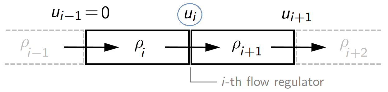
| (10) |
where is the terminal cost functional, is the running cost functional, and is the outflow constraint set associated with the -th controller. The set is obtained by relaxing any constraint involving non-local variables. From the solutions to (10), only is kept for implementation and the remaining variables () are discarded. As mentioned before, we would like to implement the solution to (10) in the form of a static state-feedback of local states as (9). The feedback realization of the solution is crucial as the values of and are affected by the action of the other controllers in the network.
The proposed decentralization scheme relies on the following properties:
- •
Existence of a global optimizer for the centralized problem with a state-feedback realization (not necessarily in a closed form).
- •
Separability of the centralized optimization problem such that a well-defined local version of the centralized optimal control problem can be constructed for each sub-network for which a global optimizer can be found in a feedback form.
IV Traffic Network
In recent years, due to the ever-increasing traffic demand, efficient control and management of transportation networks has received a great deal of attention. There has been a lot of research done on the optimal control of freeway networks based on various models for traffic systems, among which first-order models, such as the CTM, are widely used for control design. In a CTM-based traffic model, the network dynamics is described by (4), where [veh/mi] is the traffic density, [veh/hr] is the inflow rate, [veh/hr] is the outflow rate, and [mi] is the length of cell . The constraints are defined in terms of demand and supply functions, where the demand function returns the maximum outflow from the cell as a function of its current traffic density, and the supply function gives the maximum inflow into the cell as a function of its current traffic density [2]. The demand and supply functions are assumed to be of the form
| (11) |
where is continuous non-decreasing function of with and is continuous non-increasing function of with , and [veh/hr] is maximum flow capacity of cell . The jam traffic density of cell is defined as . The functions and are often assumed to be affine of the form and , where [mi/hr] is the maximum traveling free-flow speed and [mi/hr] is the backward congestion wave traveling speed of cell . Then, in a controlled network via speed limit control, the feasible region for outflow and inflow rates are defined as [2]:
| (12) |
The flow regulation mechanism in a traffic network acts as a collection of control valves, each of which at each time can be open to the fullest extent possible, completely closed, or partially closed during the network operation.
Assumption 1
The length of cells and the time interval are chosen such that vehicles traveling at maximum speed can not cross multiple cells in one time step, i.e., , . Also, the backward congestion wave traveling speed satisfies , .
Assumption 1 is known as Courant-Friedrichs-Lèvy condition [2] which is a necessary condition for numerical stability in numerical computations. It can be easily verified that Assumption 1 together with constraints (12) ensure that at each time the density of each cell is non-negative and never exceeds the jam density.
A flow network can be represented by a directed graph, in which edges represent cells and vertices (or junctions) represent interface between consecutive cells which are the actuators’ location. The junctions can be of either of the three types defined below.
Definition 1
[2] A junction with a single incoming and a single outgoing cell is called ordinary; a junction with a single incoming cell and multiple outgoing cells is called diverge; and a junction with multiple incoming cells and a single outgoing cell is called merge.
The following definitions and notations are used throughout this section.
Definition 2
Consider a network whose topology is described by directed graph . The set of edges of corresponding to on-ramps is called the source set denoted by , and the set of edges corresponding to off-ramps is called the sink set denoted by .
At any diverge junction, the traffic flow is distributed according to a given split percentage which are estimated from historical data [20].
Definition 3
[2] The split ratio (or turning ratio) is defined as the fraction of flow leaving cell that is directed towards cell , where . If cells and are not adjacent or , is defined to be zero.
Definition 4
Let cell be an incoming cell to junction , where denotes the head or the downstream junction of cell . The set of all outgoing cells from junction is called the out-neighborhood of cell and is denoted by . If , then is the empty set. In other words, is the set of all direct successor of cell . The elements of are referred to as the out-neighbors of cell .
Definition 5
Let cell be an outgoing cell from junction , where denotes the tail or the upstream junction of cell . The set of all incoming cells to junction is called the in-neighborhood of cell and is denoted by . If , then is the empty set. In other words, is the set of all direct predecessor of cell . The elements of are referred to as the in-neighbors of cell .
An example is shown in Figure 5 clarifying the above definitions.

It is often more convenient to express the dynamics and constraints in terms of the traffic mass of the cells. Let [veh] denote the traffic mass of cell at time , then from (4) and (12), the dynamics and constraints of an -cell network can be written as
| (13a) | ||||
| (13b) | ||||
| (13c) | ||||
| (13d) | ||||
where is an exogenous inflow rate to cell (, if ), and ’s are split ratios. Then, for any , , and for any , .
Remark 3
To ensure that is a feasible exogenous input to the network, it is typically assumed that the jam traffic density of any on-ramp is infinity, , and , .
Control Objective: Consider the network dynamics (13) and let be the state vector and be the control input vector of the network at time . The control objective is to design a static feedback control law such that for any initial state and any exogenous inflow , the feasibility of control actions is guaranteed and a performance index of the form (5), subject to (13) and a given information structure, over a fixed given control horizon is optimized. In this paper, we focus on linear objective functions, i.e. (5) with
| (14) |
where is a fixed final time, and and are cost-weighting parameters.
Remark 4
There are meaningful performance indexes which can be expressed in a linear form [2, 3, 4]; for example:
- (i)
Minimization of the total travel time of the network is equivalent to minimization of the total number of vehicles in the entire network, then the corresponding cost is .
- (ii)
Maximization of the total travel distance is equivalent to maximization of the flows, then the following cost should be minimized .
- (iii)
The total congestion delay is defined as the time difference between actual travel time and the travel time in free-flow conditions whose minimization is equivalent to minimizing .
For the centralized control, there is no information constraint and the control law is of the form . For the decentralized control, we consider controller with a one-hope information structure as defined below.
Definition 6
A feedback controller is said to have a one-hop information structure, if depends only on and the state of the cell(s) immediately downstream of cell , i.e. those either entering or leaving the downstream junction of cell .
For the network in Figure 5, a decentralized static feedback controller with a one-hop information structure is of the form: , , , , , and .
IV-A Centralized Feedback Control
The external inflow rate to the network acts as an exogenous input which cannot be manipulated by the controller. The solution to the optimization problem (5), (13), (14) depends, in general, on the values of ; however, no a priori knowledge on is often available for control design. Analogous to the standard LQR problem where no uncontrolled exogenous input is assumed for optimal control design, we design a centralized optimal controller under the assumption of , ; and we refer to the resulting controller as zero- optimal control law. Then, we show that the feasibility of the optimal solution in guaranteed for any nonzero .
Let us first suppose that the sequence of , over the control horizon is known beforehand. The following theorem gives the true optimal control law.
Theorem 2
The solution to (5), (13), (14) can be expressed in the form of a continuous piecewise affine static feedback law on polyhedra of the state vector as
| (15) |
where , , is the -th polyhedral partition of the set of feasible states, and is the number of polyhedral partitions at time . The controller parameters can be computed offline; they are independent of , , but may depend on the values of .
Proof: The proof is given in the Appendix.
Corollary 1
Consider the optimization problem (5), (13), (14). The zero- optimal control law can be expressed as (15), where matrices can be computed off-line. Moreover, the feasibility of the resulting control actions is guaranteed for any non-zero inflow rate , i.e., the constraints in (13) are always satisfied.
Proof: The proof is given in the Appendix.
With respect to certain cost functions, the zero- optimal feedback control law is truly optimal. We show that for problem (5), (13), (14), under certain assumptions on the network topology, if the cost functions satisfy certain properties, the centralized optimal feedback controller has a decentralized realization with a one-hop information structure which is truly optimal for any exogenous inflow .
Theorem 3
Proof: The proof is given in the Appendix.
The controller (16) has a one-hop information structure (see Definition 6); moreover, its parameters are obtain at no computational cost independent of the control horizon . Indeed, the expression in the right-hand side of (16) is the upper limit of which is known beforehand, that is , where
| (17) |
Hence, Theorem 3 states that, under the given assumptions, setting each outflow rate equal to its upper limit provides the true optimal performance. This is equivalent to opening every control valve to the fullest extent possible at each time. We refer to such scheme as trivial control or uncontrolled scheme.
Remark 5
The conditions given in Theorem 3 are sufficient (not necessary) on a linear performance index with respect to which a centralized optimal control law has a realization with a one-hop information structure. Moreover, the optimal control is not necessarily unique.
In general, however, the optimal controller needs access to the state of the entire network and depends on the control horizon. For a general network with a general linear cost functional, the closed-form of the control law (15) enables one to compute the controller parameters offline and stored in computer memory before the control actions are ever applied to the network. That is, there is no need to solve a large-size optimization problem at every time step for real-time implementation, unless there is a large variation in the network parameters. The optimal feedback controller (15), however, suffers from two major drawbacks restricting its applicability to large-scale networks: (i) Even though the piecewise affine form of the control law seems to be simple, when the number of cells and the control horizon increase, solving the corresponding multi-parametric linear programs may result in a very large number of polyhedral partitions, making the structure of the controller too complex. Although applying the merging algorithms [18, 21] may considerably reduce the number of polyhedral partitions, in general there may still be too many polyhedral sets. (ii) Determining the optimal control action at each time involves centralized operations, that is each local controller needs instantaneous access to the state of the entire network; this, however, may not be feasible for large-size networks, as implementation of a highly reliable and fast communication system may be impractical or too costly. It is, therefore, necessary to design an feedback control law with a simple structure that requires access only to local information, while providing a satisfactory performance level.
IV-B Decentralized Feedback Control
In this subsection, the objective is to design a static state-feedback control law with a one-hop information structure for problem (5), (13), (14). Such a control law, for a general network, is of the form
| (18) |
where denotes the set of all cells, excluding cell , leaving/entering the downstream junction (head) of cell . From the definition of , it follows that ; also, for any , . For example, in Figure 5, and .
Design of a decentralized feedback controller can be viewed as solving an uncertain optimization problem, wherein non-local variables/parameters are unknown. The main challenges are how to ensure the feasibility of the solution and how to express or implement it in a feedback form.
Uncertain linear program has been the subject of a lot of research and several approaches have been proposed to deal with robust optimization problems [22] including: solving the problem for nominal values of the unknown parameters and then performing sensitivity analysis; formulating the problem as a stochastic optimization by incorporating the knowledge on the probability distribution of the uncertain parameters; and assigning a finite set of possible values to the uncertain parameters and determining a solution which is relatively good for all the scenarios [23]. Also, some research has focused on evaluating the impact of uncertainty on the cost by computing the worst and best optimum solutions [24]. In some other works, in order to ensure the feasibility of solution, a worst-case approach is considered which, in general, leads to extremely conservative solutions [22].
In this paper, we follow the decentralized procedure proposed in Section III which lead to a simple decentralized control law with the desired information structure and provides a feasible solution that under certain conditions could provide the optimal centralized performance.
In order to design the -th control law with a one-hope information structure, we design a centralized optimal static state-feedback controller for the sub-network consisting of cells and any , with zero inflow rate to cell . Then, the -th local optimization is
| (19) | ||||
where
| (20) |
and the constraint set is defined by (13) with , , wherein any constraint involving non-local variables are relaxed.
Theorem 4
Proof: The proof is given in the Appendix.
We refer to (21) as a “sub-optimal decentralized control law with a one-hope information structure”. It should be highlighted that the separability property of the objective function and constraints has enabled us to simply construct a local version of the centralized optimization problem as (19).
The natural question that arises is how to evaluate the performance and sub-optimality level of the above decentralized control scheme. As mentioned earlier, in general, performance analysis of decentralized controllers is a very difficult task. Due to the lack of analytical tools, performance evaluation can be done through extensive numerical simulations. It should be noted that although the above decentralization procedure involves relaxations that may affect the conservativeness of the solution, under certain conditions, performance degradation due to decentralization is zero. It can be easily verified that if the conditions in Theorem 3 are satisfied, solving the local optimization (19) gives the true optimal controller.
Example 1
To illustrate the decentralization process, let us consider a 3-cell network

with the following cost function and constraints
| (22) |
In a decentralized control with a one-hop information structure, given local state at time , the control action at time , is obtained as follows.
| Local optimization at time | Action to be implemented |
|---|---|
|
, , , , , |
|
|
, , , , , |
|
|
, , |
V Gas Network
Consider a natural gas distribution network, where gas is transported through horizontal pipes. Flow regulation in gas networks is typically done by means of compressors and/or control valves. Transmission of natural gas over long distances and meeting consumers demand required the use of compressors to increase the pressure and to overcome pressure loss caused by friction in pipes. Also, in the distribution part of the network or where pipelines have low pressure limits, control valves are used to reduce pressure and restrict gas flow rate [10].
The problem of regulating flow in a gas network (e.g. to minimize the total supply cost) is often formulated as an optimization problem subject to nonlinear flow-pressure relations [7, 25, 26]. A controlled natural-gas pipeline system is partitioned into multiple cells as illustrated in Section I, and the gas flow dynamic for the -th cell is described by (4), where is the gas mass density [lb/ft] of cell , [lb/sec] is the inflow rate to cell , [lb/sec] is the outflow rate from cell , and is the length [ft] of cell . From the ideal gas law, the pressure in cell is given by , where is a positive constant [27]. Then, one may express the gas flow dynamic in terms of internal pressures as , where is a positive constant dependent on the physical characteristics of the pipeline.
If there is no regulator at the interface between cells and (passive interface), the flow rate from cell to the downstream cell satisfies the nonlinear equation , where is a constant characterizing the pressure drop due to flow in the pipe which is dependent upon the pipe physical characteristics (diameter, length, rugosity) [26]. In the presence of a regulator (active interface), however, the flow and pressures satisfy for a compressor, and for a control valve.
For the sake of simplicity, we focus on gas networks with a line structure as shown in Figure 2, where cells are increasingly numbered from upstream to downstream. In addition, we assume that the gas flow is regulated by control valves such that all pressure/flow constraints are met. We consider a cost function of the form
| (23) |
where is the exogenous inflow to the network coming from the high-pressure part of the network, is the purchase price of the gas, is pressure drop in the -th control valve, and is a cost-weighting parameter. The objective is to minimize the cost in (23), subject to
| (24a) | ||||
| (24b) | ||||
| (24c) | ||||
| (24d) | ||||
| (24e) | ||||
where and are known limits on the flow rate and pressure of cell , is a known upper limit for pressure drop in the -th control valve, is the outflow rate (consumer demand flow) which is known over the control horizon, denotes the output pressure of the network, and control variables are , for and .
Unlike the highway traffic problem (5), (13), (14) which is a linear program (LP), the optimization problem (24) has nonlinear inequality constraints (24b), making it non-convex and difficult to design a globally optimal feedback solution. There are numerous convexification/approximation techniques to deal with non-convex nonlinear programs (NLPs). Linear approximation, for instance, is a standard and widely-used technique in nonlinear programming. In order to find an approximate solution to (23), (24) in a feedback form, we convert it into an LP. Two approximations techniques are considered:
- •
LP1: A convexification of (24b) that makes it linear and guarantees feasibility of the approximate optimizer with respect to the original problem
- •
LP2: Through piecewise-affine approximation of the nonlinear terms in (24b), an approximate solution is obtained that provides an approximation to the global optimum cost value which can be made arbitrarily close to the true global optimum cost value by improving the approximation quality (increasing the number of breakpoints). The approximate optimizer, however, is not guaranteed to be feasible.
We use the solution to LP1 for implementation (which satisfies all the constraints) and use the optimum cost value of LP2 to evaluate the level of sub-optimality of the solution to LP1. Procedures for constructing LP1 and LP2 are described below.
We consider the following convexification to make LP1. From (24c), (24e), pressures satisfy , then the relation holds. Then, in (24b), the upper limit of can be replaced by a more conservative bound, i.e. , or equivalently , reducing (23), (24) into an LP whose solution can be expressed in a feedback form (see Theorem 1). The feasibility of solution to LP1 is guaranteed as the constraint set of LP1 is a subset of that of the original problem.
In order to assess the sub-optimality of the solution to LP1, we construct LP2 as follows. Since the nonlinear terms in (24b) are mathematically independent, one may replace each nonlinear term with a piecewise-affine approximation and utilize separable programming technique [28]. The linearization procedure and the underlying assumptions are summarized below.
Algorithm 1
[29][§10.4] (Piecewise Linear Approximation of a Separable Nonlinear Program) Consider the problem of minimizing a real-valued function over a closed and bounded region , and assume that the following properties hold:
- (i)
Every decision variable is bounded from below and above by known constants, i.e. , .
- (ii)
Decision variables appear separately in the cost and constraints, i.e. and , , can be expressed as a sum of functions of a single variable: and .
Then, the NLP in the -space is transformed into an approximate linear program (ALP) in -space as follows: For each decision variable , consider breakpoints (not necessarily equally spaced) , then express each decision variable in terms of breakpoints as
| (25) |
where , , is column vector of ones, and is the vectors of breakpoints for variable . Therefore, in the -space, the cost function and constraints can be written as
where and are respectively vectors of and evaluated at the breakpoints of . The approximation quality can be improved arbitrarily by increasing the number of breakpoints or by a suitable selection of breakpoints distribution for each nonlinear term.
The important questions in connection with Algorithm 1 are: (i) whether the solution to an ALP is feasible with respect to the original problem; and (ii) if a solution to the ALP is an approximate global (not local) optimum to the original problem. The following lemma states that the answer to the both questions is yes, if the original problem is convex.
Lemma 1
[28, 29] Consider a separable NLP as described in Algorithm 1, ans assume that and , , are separable convex functions, for some convex functions and . An optimal solution to an ALP (obtained using any standard LP solver) gives a feasible approximation to global optimizer of the original problem. Moreover, the accuracy of the solution is arbitrarily improved by increasing the number of breakpoints for each decision variable .
It should be noted that in Lemma 1, there is no need to enforce any modification such as adjacency restriction (see [28], [29][§10.4]) to standard LP solvers when solving the ALP. In general, however, applying separable programming (with or without adjacency restriction) to a non-convex problem may give an approximation to a local optimizer or an infeasible solution with respect to the original problem.
The following lemma gives some properties of concave minimization. These properties are useful to determine the optimal cost value for the gas network problem (23), (24), wherein the cost function is linear (hence both convex and concave).
Lemma 2
Consider the problem of minimizing a real-valued continuous concave function over a closed and bounded (possibly non-convex) region . Then, (i) attains its global minimum over any closed and bounded set; (ii) , where denotes the convex hull of ; (iii) attains its global minimum at an extreme point of .
Proof: (i) Since is a continuous function, then the existence of a global minimizer over any compact (closed and bounded) set follows from the well-known Weierstrass Theorem. For the proof of (ii) and (iii), see [30, Proposition 2.3] and [31, Theorem 32.2], and [32, Theorem 1.19].
From Algorithm 1 and Lemma 2, it follows that solving an ALP associated with problem (23), (24) using any standard LP solver (e.g. standard simplex method with no modification) provides an approximation to the global optimum cost value; moreover, the approximation error is arbitrarily reduced by increasing the number of breakpoints. The optimizer, however, may not be feasible as it belongs to not .
V-A Centralized Feedback Control
As mentioned earlier, in order to design a centralized feedback control law for the optimal control problem (23), (24), we replace (24b) with and solve the LP by following the same procedure explained in Section IV. Hence, the sub-optimal solution is expressed as
which is guaranteed to be feasible but may bot be truly optimal. To evaluate the level of sub-optimality of the solution we solve the corresponding LP2 problem. The linearity of the cost function and separability of the nonlinear constraints (24b) ensures that solving an ALP gives an approximation to the global optimum cost value. Comparing the optimal cost values of LP1 and LP2 gives the error introduced due to convexification in LP1.
Remark 7
For any convex problem, applying LP2 gives a feasible approximate to global optimum; hence, for flow networks with any convex objective function and constraint set one can design an optimal controller in a feedback form.
V-B Decentralized Feedback Control
By following the same procedure as that is Section IV-B, we can design a decentralized control law with a one-hop information structure for problem (23), (24), we follow and solve the LP1 associated with each sub-network and convexification errors can be found by solving the corresponding LP2.
From (24), the feasibility of depends on the values of and and is independent of the state of non-local variables. Hence, in a decentralization feedback control law with a one-hop structure, the feasibility of is ensured in the -th local optimization problem.
VI Numerical Simulation
As mentioned earlier, it is generally difficult to analytically evaluate performance of a decentralized control scheme in compared with that of an optimal centralized controller, hence comprehensive numerical simulations must be performed to demonstrate the effectiveness of a decentralization technique and and numerically assess the level of sub-optimality.
Simulation 1: Consider the 3-cell network in Example 1, with initial state . Figure 7 shows the optimal cost value for different values of control horizon , for three schemes: (i) Uncontrolled, i.e. at each time setting every control variable to its maximum possible value, (ii) Decentralized control with one-hop information structure, and (iii) Centralized control. In this example, for short control horizons , there is no performance loss due to decentralization. For , there a relative error between the performance of centralized and decentralized schemes. For larger values of , the performance of the three schemes converge to each other (for , the network is almost evacuated).

It should be noted that the uncontrolled scheme (trivial control) has a decentralized form with a one-hop information structure, but it is obtained by setting each decision variable to its maximum allowed value involving no local optimization and computational cost.
Simulation 2: To evaluate the performance of the decentralized scheme, let us consider a larger network with more realistic architecture and parameters. We consider the freeway system of an area in the southern Los Angeles as shown in Figure 8(a) modeled by the CTM. The directed graph of the network of the region of interest consisting of 32 cells is shown in Figure 8(b).

Consider minimization of , subject to (13), with the following parameters: The sampling time is hr (or sec). For on-ramp cells, the jam traffic density is assumed to be infinity and for other cells veh/mi. For all cells, the backward congestion wave traveling speed is mi/hr. For cells , the cell’s length is mi, the free-flow speed is mi/hr, and the maximum flow capacity is veh/hr, and for other cells, mi, mi/hr, and veh/hr. At any diverge junction, with incoming cell , the turning ratios are time-invariant and are split uniformly between the outgoing cells, i.e., , where is the number of outgoing cells from junction . Let be the cos weighting vector, where is the weight associated with the state of cell in cost function. We assign random integers between and to ’s and compute the optimal cost value of the centralized controller and that of the decentralized one (with one-hop information structure) , and then evaluate the relative decentralization performance loss . For example, with , we have . We consider random weighting vectors, , and for each case evaluate the relative performance loss . Figure 9 shows the histogram of the relative errors, wherein for of weighting vectors, the relative decentralization performance loss is less than .

VII Conclusion
This paper provides some structural insights into the finite-horizon optimal feedback control for flow networks. The enabling tool for the design of an optimal feedback control law is the multi-parametric linear program. It is well known that for large-size complex networks, the prohibitive computation and computation loads makes the design and implementation of a centralized controller too costly or impractical; moreover, the effect of noise, delay, or any type of error or failure in data transmission may substantially degrade the control quality. It is, therefore, necessary to develop decentralized feedback controllers with simple structure. A simple procedure is proposed to design a decentralized feedback control with a “one-hop” information structure. Moreover, it is shown that the optimal feedback controller with respect to certain linear performance indexes possesses a one-hop information structure, making the optimal controller suitable for practical implementations in large-scale networks. This suggests that if certain conditions are satisfies, the trivial control (with the least computational/communication cost) can provide the same (or very close) performance to that of the centralized control (with the most computational/communication cost).
For a given flow network of size and control horizon , it is invaluable to analytically determine when it is worth to implement uncontrolled scheme, or a decentralized control law with a -hop information structure to achieve a satisfactory level of permanence. Our ultimate objective is to develop a principled approach for distributed optimal control of physical infrastructure networks under given information constraints.
Appendix
Proof of Theorem 2: The proof follows by following a similar procedure as that in [33, §2]. The closed-form solution to (13a) starting from initial state is given by
| (26) |
where from (13b), the total inflow rate to cell at time is
| (27) |
where denotes the tail (upstream junction) of cell . Then, from (5), (14), (26), and (27), the cost function can be expressed as a linear combination of ’s as follows:
Then, the cost function over horizon can be written as
| (28) |
where
| (29) |
and the coefficients of the decision variables are given by
| (30) |
From (13b) and (27), if the head (downstream junction) of cell is either ordinary or diverge, the constraint for is
| (31) |
and if the head of cell is a merge junction with , then must satisfy
| (32) |
Due to the linearity of the objective function (28) and constraints (31)-(32), the optimization problem can be expressed as a multi-parametric linear program of the form (6), wherein the state vector at time , i.e., , is treated as a varying parameter vector in the optimization problem, and the decision variable vector contains the control actions for , i.e., . From Theorem 1, we have
which can be expressed as
| (33) |
where is the -th row of matrix and is the -th element of vector . The above results imply that when optimizing the performance index starting at over the control horizon , i.e., with parameter vector , then the optimal solution (33) provides a static state-feedback optimal control law only at the initial time , i.e.,
Hence, to design a feedback control law, we retain only the first equation in (33) and discard the rest of them. Therefore, in (15), the parameters of the optimal feedback controller at time are given by
| (34) |
The optimal value of when is applied to the system gives an optimal value of , then at the next time step by repeating the same procedure starting at the initial time over the control horizon with as a parameter vector, we can express the optimal value of as a piecewise affine function of . Therefore, in general, optimizing the performance index over the time interval , i.e., with parameter vector and decision variable vector , provides a state-feedback optimal control law at time step in the form of a piecewise affine function on polyhedra of , for any . Hence, by solving multi-parametric linear programs, the optimal feedback controller can be expressed as (15).
Proof of Corollary 1: The proof of the first part immediately follows from Theorem 2. The state of an on-ramp is given by . Since only the state of an on-ramp cell directly depends on exogenous inflow rates, we need to just check the constraints that depend on for . From (13), the only constraint depending on the state of on-ramps is , , which can be written as . Since the last term on the right side of the inequality is non-negative, the feasibility of zero- optimal solution is guaranteed, when it is applied to a network with nonzero .
Proof of Theorem 3: From (28) and (31), for a network with no merge junction we can write
| (35) |
From the definition of split ratios, is a convex combination of ’s, for all , and under the assumptions on the cost-weighting parameters, i.e., , and , and , , and that the split ratios are time invariant, it follows that , .
By using the dynamic programming approach [34, §6.2], we show that under the above assumptions, an optimal solution is obtained when each decision variable is set equal to its upper limit defined in (31). For the maximization problem (35), we define the objective functional over the time interval starting at time from initial state as
| (36) |
Then, the corresponding functional equation of dynamic programming is given by
| (37) |
where denotes the optimal value of the objective function over the time interval from initial state . Hence, the optimization over the horizon is converted into optimization over only one control vector at a time by working backward in time for . The optimization problem (37) is a bound constrained optimization problem, hence if we show that is an increasing function of (i.e., increasing in every coordinate ), , then is an optimum solution.
For a one-stage process with initial state , the -function is
| (38) |
Since , , then is an increasing function of , , then .
For a two-stage process with initial state , the -function is
| (39) |
From , (31), and , where is the only in-neighbor of cell (see (27)),
| (40) |
where , . By multiplying both sides of (40) by and adding to the both sides we obtain
| (41) |
where and , . Since and , then , . From (39) and (41), and that the coefficients of are non-negative , and using the fact that the minimum and the sum of increasing functions are also increasing, it follows that is an increasing function of , then , , is an optimal control action.
For a -stage process with initial state , assuming that , for , the -function is given by
| (42) |
From (31) and that , we have
| (43) |
where is the only in-neighbor of cell and , for . By multiplying both sides of (43) by and then adding to the both sides (wherein , for ), we obtain
| (44) | ||||
where and , . Since and , then and , and any .
Due to the non-negativity of the coefficients of in the right-hand side of (44), is maximized if the terms , , and are maximized, , and so on, where be a generic symbol for a sequence of parameters satisfying , . The above recursion implies that , , is an optimal solution.
Therefore, the optimum control is independent of the control horizon and external inflow rates , and is obtained at no computational cost by setting each equal to its known upper limit , (given that is known at time ). From the expression for , it follows that the true optimal outflow rate is found by measuring only and .
Proof of Theorem 4: Since the decentralized controller is obtained by solving a centralized problem for a sub-network consisting of cell and , then the proofs follows from Theorem 2 and Corollary 1. The feasibility of in (21), , follows from the proof of Theorem 2 and that from (31) and (32), at each time , the feasibility of depends on the values of and , and is independent of the state of non-local variables. Hence, the feasibility of is ensured in the -th local optimization problem.
References
- [1] B. R. Munson, A. P. Rothmayer, T. H. Okiishi, and W. W. Huebsch, Fundamentals of Fluid Mechanics. John Wiley & Sons, Inc., 2012.
- [2] G. Como, E. Lovisari, and K. Savla, “Convexity and robustness of dynamic traffic assignment and freeway network control,” Transportation Research Part B: Methodological, vol. 91, pp. 446–465, 2016.
- [3] Y. Han, A. Hegyi, Y. Yuan, S. Hoogendoorn, M. Papageorgiou, and C. Roncoli, “Resolving freeway jam waves by discrete first-order model-based predictive control of variable speed limits,” Transportation Research Part C: Emerging Technologies, vol. 77, pp. 405–420, 2017.
- [4] A. Muralidharan and R. Horowitz, “Computationally efficient model predictive control of freeway networks,” Transportation Research Part C: Emerging Technologies, vol. 58, pp. 532–553, 2015.
- [5] C. Daganzo, “The cell transmission model: A dynamic representation of highway traffic consistent with the hydrodynamic theory,” Transportation Research Part B, vol. 28, no. 4, pp. 269–287, 1994.
- [6] L. Adacher and M. Tiriolo, “A macroscopic model with the advantages of microscopic model: A review of cell transmission model’s extensions for urban traffic networks,” Simulation Modelling Practice and Theory, vol. 86, pp. 102–119, 2018.
- [7] P. Wong and R. Larson, “Optimization of natural-gas pipeline systems via dynamic programming,” IEEE Transactions on Automatic Control, vol. 13, no. 5, pp. 475–481, 1968.
- [8] S. Misra, M. W. Fisher, S. Backhaus, R. Bent, M. Chertkov, and F. Pan, “Optimal compression in natural gas networks: A geometric programming approach,” IEEE Transactions on Control of Network Systems, vol. 2, no. 1, pp. 47–56, 2015.
- [9] A. Martin, M. Möller, and S. Moritz, “Mixed integer models for the stationary case of gas network optimization,” Mathematical Programming, vol. 105, no. 2, pp. 563–582, 2006.
- [10] T. Koch, B. Hiller, M. Pfetsch, and L. Schewe, Evaluating Gas Network Capacities. Philadelphia, PA: Society for Industrial and Applied Mathematics, 2015.
- [11] A. Hegyi, B. D. Schutter, and H. Hellendoorn, “Model predictive control for optimal coordination of ramp metering and variable speed limits,” Transportation Research Part C: Emerging Technologies, vol. 13, no. 3, pp. 185–209, 2005.
- [12] I. Papamichail, A. Kotsialos, I. Margonis, and M. Papageorgiou, “Coordinated ramp metering for freeway networks– A model-predictive hierarchical control approach,” Transportation Research Part C: Emerging Technologies, vol. 18, no. 3, pp. 311–331, 2010.
- [13] M. Hadiuzzaman and T. Z. Qiu, “Cell transmission model based variable speed limit control for freeways,” Canadian Journal of Civil Engineering, vol. 40, no. 1, pp. 46–56, 2013.
- [14] J. Tsitsiklis and M. Athans, “On the complexity of decentralized decision making and detection problems,” IEEE Transactions on Automatic Control, vol. 30, no. 5, pp. 440–446, 1985.
- [15] R. Cogill, M. Rotkowitz, B. V. Roy, and S. Lall, “An approximate dynamic programming approach to decentralized control of stochastic systems,” in Control of Uncertain Systems: Modelling, Approximation, and Design. Springer Berlin Heidelberg, 2006, pp. 243–256.
- [16] H. Lakshmanan and D. P. de Farias, “Decentralized approximate dynamic programming for dynamic networks of agents,” in 2006 American Control Conference (ACC), June 2006, pp. 1648–1653.
- [17] F. Borrelli, Constrained Optimal Control of Linear and Hybrid Systems. Springer, 2003.
- [18] M. Herceg, M. Kvasnica, C. N. Jones, and M. Morari, “Multi-Parametric Toolbox 3.0,” in Proc. of the European Control Conference, Zürich, Switzerland, July 17–19 2013, pp. 502–510. [Online]. Available: http://control.ee.ethz.ch/~mpt
- [19] J. Lofberg. YALMIP: A toolbox for modeling and optimization in MATLAB. [Online]. Available: https://yalmip.github.io/download/
- [20] J. Krumm, “Where will they turn: predicting turn proportions at intersections,” Personal and Ubiquitous Computing, vol. 14, no. 7, pp. 591–599, 2010.
- [21] M. Baotic, F. J. Christophersen, and M. Morari, “A new algorithm for constrained finite time optimal control of hybrid systems with a linear performance index,” in 2003 European Control Conference (ECC), 2003, pp. 3323–3328.
- [22] D. Bertsimas and A. Thiele, “A robust optimization approach to inventory theory,” Operations Research, vol. 54, no. 1, pp. 150–168, 2006.
- [23] V. Gabrel, C. Murat, and N. Remli, “Linear programming with interval right hand sides,” International Transactions in Operational Research, vol. 17, no. 3, pp. 397–408, 2010.
- [24] J. W. Chinneck and K. Ramadan, “Linear programming with interval coefficients,” The Journal of the Operational Research Society, vol. 51, no. 2, pp. 209–220, 2000.
- [25] P. Wong and R. Larson, “Optimization of tree-structured natural-gas transmission networks,” Journal of Mathematical Analysis and Applications, vol. 24, no. 3, pp. 613–626, 1968.
- [26] D. D. Wolf and Y. Smeers, “The gas transmission problem solved by an extension of the simplex algorithm,” Management Science, vol. 46, no. 11, pp. 1454–1465, 2000.
- [27] A. Zlotnik, M. Chertkov, and S. Backhaus, “Optimal control of transient flow in natural gas networks,” in 2015 54th IEEE Conference on Decision and Control (CDC), Dec 2015, pp. 4563–4570.
- [28] S. M. Stefanov, Separable Programming: Theory and Methods. Springer, Boston, MA, 2001.
- [29] P. A. Jensen and J. F. Bard, Operations Research Models and Methods. John Wiley & Sons, Inc., 2003.
- [30] W. W. Hager, D. T. Phan, and J. Zhu, “Projection algorithms for nonconvex minimization with application to sparse principal component analysis,” Journal of Global Optimization, vol. 65, no. 4, pp. 657–676, 2016.
- [31] R. T. Rockafellar, Convex Analysis. Princeton University Press, 1970.
- [32] R. Horst, P. M. Pardalos, and N. V. Thoai, Introduction to Global Optimization. Springer, US, 2000.
- [33] F. Borrelli, “Discrete time constrained optimal control,” Ph.D. dissertation, Swiss Federal Institute of Technology (ETH) Zurich, 2002.
- [34] F. L. Lewis, D. L. Vrabie, and V. L. Syrmos, Optimal Control. John Wiley & Sons, Inc., 2012.