Gluing together Modular flows with free fermions

To keep things simple, we begin with two symmetrically placed intervals $V=(-b,-a)\cup(a,b)$ on the real axis of the complex $z$ plane. The aforementioned obstruction can be nicely illustrated by trying to map the half-line modular flow of figure 1 into the two-interval modular flow of figure 2 via the mapping

$\displaystyle w=f(z)=\frac{(z+b)(z-a)}{(z+a)(z-b)},$

(10)

as discussed in [11]. This mapping is two to one, with branch point singularities at

$\displaystyle z_{\pm}=\pm i\sqrt{ab}$

(11)

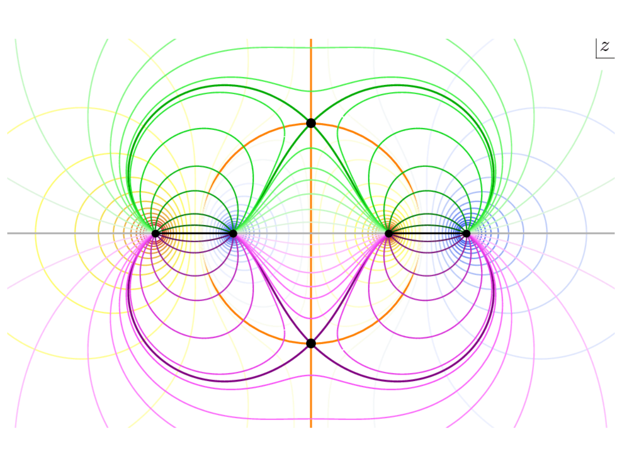
where it is one to one and fails to be conformal because the derivative vanishes there. This means that if we try to lift the half line modular flow on the $w$ plane to the $z$ plane we will find two singularities at $z_{\pm}$, in addition to the usual ones at the entangling surface $\partial V$. The field lines of this two-interval modular flow is shown in figure 2, borrowed from [11]. While the singularities at $\partial V$ can be regulated by cutting out small disks, the singularities at $z_{\pm}$ present an obstruction to the naive, local modular flow generated by (5). Indeed, if we carefully follow the evolution of the constant time slices (green and purple lines) in figure 2, we see that as the two intervals approach the singularities $z_{\pm}$, they are cut and reconnected so that right endpoint of the left interval becomes connected with the left endpoint of the right interval and vice versa. This led the the authors of [11] to characterized the two- interval reduced density matrix $\rho_{V}$ by the sequence of operators:

$\displaystyle\rho_{V}=e^{-\theta_{0}K_{V}}X^{\dagger}e^{-(2\pi-2\theta_{0})K_{\bar{V}}}Xe^{-\theta_{0}K_{V}}$

(12)

Here $K_{V}$ and $K_{\bar{V}}$ generate a geometric flow that evolve regions $V$ and $\bar{V}$ in the angular coordinate $\theta$ which runs orthogonal to $V$ and $\bar{V}$: these operators are given by the integral of the stress tensor over regions $V$ and $\bar{V}$ respectively, similar to (5). The “cutting and regluing” operators $X$ and $X^{\dagger}$ are inserted at $z_{\pm}$: they map from the Hilbert space $\mathcal{H}_{V}$ to the complement $\mathcal{H}_{\bar{V}}$ and vice versa, allowing the continuation of the modular flow past the singularities at $z_{\pm}$ by switching back and forth between evolution by $K_{V}$ and $K_{\bar{V}}$. To obtain the modular Lagrangian, we must incorporate the effects of $X$ and $X^{\dagger}$ into the path integral. Below we will show how this can be done by orbifolding the complex $z$ plane and imposing twisted boundary conditions. These boundary conditions will generate the bilocal term in the Modular Hamiltonian (7), and can be interpreted as a gluing of the single interval modular flows that entangles the disjoint intervals.

We begin with the key observation that the mapping (10) is single valued provided we treat $w$ like a local coordinate on a Riemann surface $\Sigma_{2}$, which is a two fold branched cover of the $w$-plane (right of figure 3). The two branch points in this covering corresponding to $z_{\pm}$ are located at

$\displaystyle w_{\pm}=-(\frac{\sqrt{a}\mp i\sqrt{b}}{\sqrt{a}\pm i\sqrt{b}})^{2}.$

(13)

In this coordinate system, $V$ consists of two copies of the half infinite line $\mathbb{R}^{+}$ living on the two sheets, and the two-interval modular flow is mapped to the simultaneous evolution of these two half lines that sweeps out the surface $\Sigma_{2}$. This evolution starts off as a simultaneous rigid rotation, but is then interrupted by the presence of the branch point joining the two sheets. The branch point cuts and re-glues the two half lines as shown in the figure 4. This is the same cutting and re-gluing process described earlier on the $z$ plane, except that the process is automatically implemented by the topology of $\Sigma_{2}$.

The advantage of working in the $w$ coordinate system is that the effects of the branch points can be represented by the type of twisted boundary conditions that appears in orbifold CFT’s. To do this, we orbifold the surface $\Sigma_{2}$ by identifying points on the two sheets with the same $w$ coordinate. This leads to a theory of two “replica” fields $\Psi_{1}(w),\Psi_{2}(w)$ on a single-sheeted surface with nontrivial monodromies around $w_{\pm}$ :

	$\displaystyle\Psi_{1}(e^{2\pi i}w_{+})$	$\displaystyle=\Psi_{2}(w_{+})$
	$\displaystyle\Psi_{2}(e^{2\pi i}w_{+})$	$\displaystyle=-\Psi_{1}(w_{+})$		(14)
	$\displaystyle\Psi_{1}(e^{2\pi i}w_{-})$	$\displaystyle=-\Psi_{2}(w_{-})$
	$\displaystyle\Psi_{2}(e^{2\pi i}w_{-})$	$\displaystyle=+\Psi_{1}(w_{-})$		(15)

Note the minus sign in the second and third equation due to the rotation of the fermion around the branch points. Assuming identical boundary conditions for $\Psi_{1}$ and $\Psi_{2}$ at the regulator surfaces near $w=0$ and $w=\infty$, the monodromies can be diagonalized by defining

$\displaystyle\Psi_{\pm}=\frac{1}{\sqrt{2}}(\Psi_{1}\pm i\Psi_{2}),$

(16)

which satisfy

	$\displaystyle\Psi_{\pm}(e^{2\pi i}w_{+})$	$\displaystyle=\pm i\Psi_{+}(w_{+})$
	$\displaystyle\Psi_{\pm}(e^{2\pi i}w_{-})$	$\displaystyle=\mp i\Psi_{+}(w_{+})$		(17)

The effective partition function $Z_{V}=\tr_{V}e^{-H_{V}}$ can be express by the path integral

	$\displaystyle Z_{V}$	$\displaystyle=\int[D\Psi_{\pm}D\bar{\Psi}_{\pm}]_{\text{twisted}}e^{-S[\Psi_{\pm},\bar{\Psi}_{\pm}]}$
	$\displaystyle S$	$\displaystyle=\int\Psi_{+}\bar{\partial}\Psi_{+}+\Psi_{-}\bar{\partial}\Psi_{-}d^{2}w+\int\bar{\Psi}_{+}\partial\bar{\Psi}_{+}+\bar{\Psi}_{-}{\partial}\bar{\Psi}_{-}d^{2}\bar{w}$		(18)

where the twist boundary conditions (14) have been imposed in the measure. To obtain the modular action, we have to incorporate these boundary conditions into the action. For free fermions, this can be done by coupling $(\Psi_{+},\Psi_{-})$ to a fictitious background U(1) gauge field with holomorphic and anti holomorphic components :

$\displaystyle\mathcal{A}=\begin{pmatrix}A^{+}&&0\\ 0&&A^{-}\end{pmatrix}\quad\quad\bar{\mathcal{A}}=\begin{pmatrix}\bar{A}^{+}&&0\\ 0&&\bar{A}^{-}\end{pmatrix}$

(19)

Then the monodromies (14) can be interpreted as specifying the non-trivial parallel transport of $\Psi_{\pm}$ around $w_{\pm}$. The required gauge fluxes ¹¹ 1 Explicitly, the gauge fluxes reproducing (14) are $\displaystyle\int_{C_{+}}A^{+}$ $\displaystyle=\frac{\pi}{2},\quad\quad\int_{C_{-}}A^{+}=-\frac{\pi}{2}$ $\displaystyle\int_{C_{+}}A^{-}$ $\displaystyle=-\frac{\pi}{2},\quad\quad\int_{C_{-}}A^{-}=\frac{\pi}{2}$ (20) where $C_{\pm}$ denote counterclockwise loops encircling $w_{\pm}$. are realized by the (singular) gauge fields

	$\displaystyle A^{+}$	$\displaystyle=\frac{1}{4i}(\frac{1}{w-w_{+}}-\frac{1}{w-w_{-}})dw,\quad\quad A^{-}=-A^{+}$
	$\displaystyle\bar{A}^{+}$	$\displaystyle=-\frac{1}{4i}(\frac{1}{\bar{w}-\bar{w}_{+}}-\frac{1}{\bar{w}-\bar{w}_{-}})d\bar{w},\quad\quad\bar{A}^{-}=-\bar{A}^{+}$		(21)

Instead of imposing twisted boundary conditions in the measure for $Z_{V}$ as in (18), we couple unconstrained free fermions $\Psi_{\pm}$ to the background gauge field $\mathcal{A},\bar{\mathcal{A}}$. This defines the action

$\displaystyle S_{V}=\int_{\Sigma}\Psi_{+}\bar{\partial}\Psi_{+}+\Psi_{-}\bar{\partial}\Psi_{-}+i\bar{A}^{+}(\Psi_{+}^{\dagger}\Psi_{+}-\Psi_{-}^{\dagger}\Psi_{-})+\text{Anti-holomorphic part}$

(22)

In terms of $S_{V}$, the effective partition function becomes:

$\displaystyle Z_{V}=\int D\Psi_{\pm}D\bar{\Psi}_{\pm}e^{-S_{V}[\Psi_{\pm},\bar{\Psi}_{\pm},A^{+},\bar{A}^{+}]}$

(23)

The path integral measure is now the usual one on the $w$ plane, with no twisted boundary conditions. Note that despite the singularities in the gauge fields at $w_{\pm}$, the Lagrangian for $S_{V}$ is smooth everywhere because $A^{+},\bar{A}^{+}$ couples to the $U(1)$ currents

	$\displaystyle\mathcal{J}(w)$	$\displaystyle=\Psi^{\dagger}_{+}\Psi_{+}-\Psi^{\dagger}_{-}\Psi_{-}=i(\Psi^{\dagger}_{1}\Psi_{2}-\Psi^{\dagger}_{2}\Psi_{1})$
	$\displaystyle\mathcal{\bar{J}}\bar{(}w)$	$\displaystyle=\bar{\Psi}^{\dagger}_{+}\bar{\Psi}_{+}-\bar{\Psi}^{\dagger}_{-}\bar{\Psi}_{-}=i(\bar{\Psi}^{\dagger}_{1}\bar{\Psi}_{2}-\bar{\Psi}^{\dagger}_{2}\bar{\Psi}_{1})$		(24)

which vanish at $w_{\pm}$, where $\Psi_{1}=\Psi_{2}$. The original problem of obtaining the two -interval modular Hamiltonian is now mapped to problem of obtaining the half line modular Hamiltonian for $Z_{V}$.

Now we come to the crucial point. The expression (23) for $Z_{V}$ makes manifest a rotational invariance around the entangling surface $w=0$. This means that $S_{V}$ defines a finite temperature field theory with the angular direction around $w$ as the temperature circle, and is therefore the modular action we have been searching for. To show this, we construct the charge that generates rotations around $w=0$ and show that it is explicitly conserved. This is given by

$\displaystyle K(\theta)=\int_{V(\theta)}\,wT_{V}(w)dw+\int_{V(\theta)}\,\bar{w}\bar{T}_{V}(\bar{w})d\bar{w}$

(25)

where $V(\theta)$ is a ray leaving the origin at angle $\theta$, and $T_{V},\bar{T}_{V}$ are the components of modular stress tensor derived from the action $S_{V}$. In the original gauge, we would interpret $T_{V},\bar{T}_{V}$ as the quantum stress tensor containing a contribution path-integral measure. Note that the expression in (25) for the rotational generator assumes a traceless stress tensor, implying that $S_{V}$ also defines a conformal field theory. We will show this is indeed the case in the next section. Explicitly, we have

	$\displaystyle T_{V}$	$\displaystyle=T+iA^{+}\mathcal{J}$
	$\displaystyle\bar{T}_{V}$	$\displaystyle=\bar{T}+i\bar{A}^{+}\bar{\mathcal{J}},$			(26)

where $T,\bar{T}$ are the stress tensors for the free fermions $\Psi_{\pm}$ in the absence of the gauge field. The charge $K$ is conserved provided that $T_{V}$/$\bar{T}_{V}$ are holomorphic/anti-holomorphic ( see figure 5), which we can check explicitly.

	$\displaystyle\bar{\partial}T_{V}(w)$	$\displaystyle=\frac{1}{4}\mathcal{J}(w)\bar{\partial}\left(\frac{1}{w-w_{+}}-\frac{1}{w-w_{-}}\right)$
		$\displaystyle=\frac{1}{4}\mathcal{J}(w)\left(\delta(w-w_{+})-\delta(w-w_{-})\right)=0$		(27)

due to the vanishing of the $\mathcal{J}$ at $w_{\pm}$.

Since $K$ is conserved, we can apply (5) to get the half space modular hamiltonian on the $w$ plane:

	$\displaystyle H_{\mathbb{R}^{+}}$	$\displaystyle=\int_{\mathbb{R}^{+}}2\pi w\,T_{V}(w)\,dw$
		$\displaystyle=\int_{\mathbb{R}^{+}}2\pi w\left(\sum_{a=\pm}\frac{\Psi^{\dagger}_{a}\partial_{w}\Psi_{a}+\Psi_{a}\partial_{w}\Psi^{\dagger}_{a}}{2}+iA^{+}(\Psi^{\dagger}_{+}\Psi_{+}-\Psi^{\dagger}_{-}\Psi_{-})\right)\,dw$		(28)

To see the non-locality of this modular Hamiltonian, we rotate back to the $\Psi_{1,2}(w)$ basis and observe the coupling:

	$\displaystyle\delta H_{\mathbb{R}^{+}}$	$\displaystyle=2\pi i\int wA^{+}\left(\Psi^{\dagger}_{+}\Psi_{+}-\Psi^{\dagger}_{-}\Psi_{-}\right)\,dw$
		$\displaystyle=2\pi\int w\,\Psi^{\dagger}_{i}(w)\mathcal{A}_{ij}\Psi_{j}(w)\,dw$		(29)

where

$\displaystyle\mathcal{A}_{ij}=\frac{\epsilon_{ij}}{4}\frac{(w_{+}-w_{-})}{(w-w_{+})(w-w_{-})}$

(30)

In the $w$ coordinate system, this looks like a local coupling of two fermion fields. However, when mapped to the $z$ plane, this will become a bi-local coupling of single fermion field evaluated at two different locations.

To make a full comparison to the modular Hamiltonian (7), we now transform back to the $z$ coordinates. To do so, note that we have applied the mapping (10) as a diffeomorphism, rather than a conformal map. In particular, the singularities at $w_{\pm}$ are coordinate singularities rather than curvature singularities. This is manifest in the original $z$ plane, since the path integral defining the reduced density matrix $\rho_{V}$ was non-singular at $z_{\pm}$. Instead, $z_{\pm}$ are singularities of the two-interval foliation, which exactly matches the branch point singularities of the mapping (10). Therefore we do not need to account for the conformal anomaly when we transform back to the $z$ coordinates.

Second, note that the inverse $z=f^{-1}(w)$ is multi-valued, so we must choose a branch.

In the $z$ coordinates, orbifolding $\Sigma_{2}$ corresponds to identifying the two points ²² 2 We can think of $z_{1,2}(w)$ as coordinates on the two different sheets of $\Sigma$ $z_{1}(w)$ and $z_{2}(w)$ that are mapped to the same $w$ under (10). These are two roots of a quadratic polynomial that are related by

$\displaystyle z_{1}z_{2}=-ab$

(31)

The orbifold theory thus consists of a two component fermion field $(\Psi(z_{1}),\Psi(z_{2}))$ living on half of the $z$ plane (see region 1 in figure 6); we choose this to be the half containing the left interval $V_{1}=(-b,-a)$ and coordinatized by $z_{1}$. Given this choice, and treating $z_{2}$ as a function of $z_{1}$ given by (31), we can transform $\delta H_{\mathbb{R}^{+}}$ according to

	$\displaystyle\Psi_{1}(w)$	$\displaystyle=(\frac{dz_{1}}{dw})^{1/2}\Psi(z_{1})$
	$\displaystyle\Psi_{2}(w)$	$\displaystyle=(\frac{dz_{2}}{dw})^{1/2}\Psi(z_{2})$
	$\displaystyle dw$	$\displaystyle=\frac{dw}{dz_{1}}dz_{1}$		(32)

which gives

	$\displaystyle\delta H_{V}$	$\displaystyle=-2\pi\int_{V_{1}}\left(\frac{d\log\,w}{dz_{2}}\right)^{-1}\frac{\Psi^{\dagger}(z_{1})\Psi(z_{2})-\Psi^{\dagger}(z_{2})\Psi(z_{1})}{z_{1}-z_{2}}dz_{1},$
		$\displaystyle=-2\pi\sum_{j\neq i}\int_{V_{i}}\left(\frac{d\log\,w}{dz_{j}}\right)^{-1}\frac{\Psi^{\dagger}(z_{i})\Psi(z_{j})}{z_{i}-z_{j}}dz_{i}$		(33)

Lifting back from the orbifold to the $z$ plane, this term represents a bi local coupling of the fields at $z_{1}$ and $z_{2}$. This is the same bilocal term that appears in equation (7) and was first derived in [9]. Similarly, transforming the kinetic terms $2\pi\int w\,dw\,\left(\Psi^{\dagger}_{+}\partial\Psi_{+}+\Psi_{-}\partial\Psi^{\dagger}_{-}+\text{h.c.}\right)$ in (28) back to the $z$ plane gives the local term in the modular Hamiltonian (7).

$\displaystyle H_{V}^{\text{local}}=2\pi\int_{V}\left(\frac{d\log\,w}{dz}\right)^{-1}\left(\frac{\Psi^{\dagger}(z)\partial\Psi(z)+\Psi(z)\partial\Psi^{\dagger}(z)}{2}\right)\,dz$

(34)

Even though we have derived (33) for $\delta H_{V}$ using a particularly symmetric choice of intervals, the result holds for a general pair of intervals $V=(a_{1},b_{1})\cup(a_{2},b_{2})$. Showing this directly is tedious because solving for $z_{2}$ in terms of $z_{1}$ and $a_{i},b_{i}$ is more complicated in general, since they are the roots of the polynomial

$\displaystyle p(z)=w\prod^{2}_{i=1}(z-b_{i})-\prod^{2}_{i=1}(z-a_{i})$

(35)

However one can circumvent this calculation by noting that for generic intervals, pulling back $\delta H_{\mathbb{R}^{+}}$ via the function $z_{1}(w)$ gives

	$\displaystyle\delta H_{V}$	$\displaystyle=\int_{V_{1}}\left(\frac{d\log w}{dz_{2}}\right)^{-1}\sqrt{\frac{dz_{1}}{dz_{2}}}\mathcal{A}_{ij}\Psi^{\dagger}(z_{i})\Psi(z_{j})\,dz_{1}$		(36)
	$\displaystyle\mathcal{A}_{ij}(z_{1})$	$\displaystyle=\frac{dw}{dz_{1}}\mathcal{A}_{ij}(w),$		(37)

where $\mathcal{A}_{ij}(z_{1})$ is the gauge field implementing the monodromies (14) in the $z_{1}$ coordinate system. For the special case $V=(-b,-a)\cup(a,b)$, imposing that $\mathcal{A}_{ij}(z_{1})$ has the correct poles and residues at $z_{\pm}$ gives

	$\displaystyle\mathcal{A}_{ij}(z_{1})$	$\displaystyle=\frac{\sqrt{ab}}{2}\frac{1}{(z_{1}-i\sqrt{ab})(z_{1}+i\sqrt{ab})}$
		$\displaystyle=\frac{\epsilon_{ij}}{4}\frac{\sqrt{\frac{dz_{2}}{dz_{1}}}}{z_{1}-z_{2}},$		(38)

where in the second equality we applied (31). Moreover, this expression remains valid for arbitrary pairs of intervals, since it makes no reference to the endpoints $(a_{i},b_{i})$. Plugging this back into (36) gives the general result (33).

The modular Hamiltonian for multiple intervals can be obtained by directly generalizing the orbifold method in section $2.1$. It will be convenient to consider periodic (Neveu-Schwarz) fermions living on the unit circle in the radially quantized $z$ plane. The reduced density matrix is given by the path integral on the $z$ plane with cuts along a set of segments $V=\cup_{i}(a_{i},b_{i})$ of the unit circle. The change of coordinates

$\displaystyle w=\prod^{n}_{i=1}\frac{z-a_{i}}{z-b_{i}}$

(39)

takes the $z$ plane to a generically $n$ sheeted surface $\Sigma_{n}$ with local coordinate $w$. The $n$ sheets are labelled by the roots $z_{i}(w)$ of the polynomial

$\displaystyle f(w,z)=w\prod^{n}_{i=1}{z-b_{i}}-\prod^{n}_{i=1}z-a_{i}$

(40)

and branch points connect multiple sheets where ever the roots collide. To simplify the analysis, we consider the case where intervals are symmetrically placed around the circle, so that for $j\neq 1$

	$\displaystyle a_{j}=r^{j}a_{1}$		(41)
	$\displaystyle b_{j}=r^{j}b_{1}$		(42)
	$\displaystyle r=e^{\frac{2\pi i}{n}}$		(43)

In this case the $n$ roots are related by

$\displaystyle z_{j}(w)=r^{j}z_{1}(w)$

(44)

and there are only two branch points at $z=0,\infty$, each with multiplicity $n$. On $\Sigma_{n}$, the two branch points are located at $w_{+}=1$ and $w_{-}=e^{-iL}$, where $L$ is the total length of $V$. As before, we orbifold $\Sigma_{n}$ by identifying $z_{i}(w)$ for $i=1\cdots n$ to obtain an $n$- component field

$\displaystyle\Psi=(\Psi_{1}(w),\cdots,\Psi_{n}(w))$

(45)

with non-trivial holonnomy around $w_{-}$:

	$\displaystyle\Psi$	$\displaystyle\rightarrow T\Psi$
	$\displaystyle T=$	$\displaystyle\begin{pmatrix}0&&1&&0&&\cdots&&0\\ \vdots&&0&&1&&0&&\vdots\\ \vdots&&\vdots&&0&&\ddots&&0\\ \vdots&&\vdots&&\vdots&&\ddots&&1\\ (-1)^{n+1}&&0&&\cdots&&0&&0\\ \end{pmatrix}$		(46)

and similarly around $w_{+}$ with holonomy $T^{-1}$. As noted before, the minus sign in the lower left corner is due to the non-trivial spin of the fermion [12]. The holonomy (46) can be described as a exponential of a matrix gauge field $\mathcal{A}_{ij}$

$\displaystyle T=\exp i\int_{C_{\pm}}\mathcal{A}$

(47)

where the $C_{\pm}$ encircle $w_{\pm}$. For even $n$, $T$ is diagonal in the basis ³³ 3 For the purpose of diagonalizing the twist, we could also have written $\displaystyle\Phi_{k}(w)=\frac{1}{\sqrt{n}}\sum_{j}r^{(\frac{1}{2}-k)j}\Psi_{j}(w)$ (48) with $k=1,\cdots n$, which just permutes the eigenvectors chosen above. The corresponding transformation matrix $B_{kj}=r^{(\frac{1}{2}-k)j}$ appears in in the diagonalization of the multi-interval modular flow. The eigenvalues obviously doesn’t change. However, we have made a particular chose of phases in the expressions for $t_{k}$, which does affect the gauge fields. Even though we could in principle shift the phases by integer multiples of $2\pi$ with out change $t_{k}$ , these shifts would change Modular Hamiltonian and effectively select out a state different than the ground state.

	$\displaystyle\Phi_{k}(w)$	$\displaystyle=\frac{1}{\sqrt{n}}\sum_{j}r^{(k-\frac{n+1}{2})j}\Psi_{j}(w),$
	$\displaystyle k$	$\displaystyle=1,2,\cdots,n$		(49)

consisting of eigenvectors with eigenvalue $t_{k}=e^{\frac{2\pi i}{n}(\frac{n+1}{2}-k)}$. In this basis, $\mathcal{A}$ has diagonal entries

	$\displaystyle A_{k}=\frac{1}{n}(\frac{n+1}{2}-k)\frac{1}{i}\left(\frac{1}{w-w_{+}}-\frac{1}{w-w_{-}}\right)$
	$\displaystyle k=1,2,\cdots,n$		(50)

so that coupling term in the modular Hamiltonian analogous to (29) is

$\displaystyle\delta H_{R^{+}}$

$\displaystyle=2\pi i\int_{R^{+}}wA_{k}\Phi^{\dagger}_{k}(w)\Phi_{k}(w)\,dw$

(51)

Undoing the diagonalization then expresses this coupling in terms of an antisymmetric matrix gauge field [1]:

	$\displaystyle\mathcal{A}_{ij}$	$\displaystyle=\frac{1}{i}\left(\frac{1}{w-w_{+}}-\frac{1}{w-w_{-}}\right)\frac{-r^{\frac{i+j}{2}}}{r^{i}-r^{j}}$
	$\displaystyle i$	$\displaystyle\neq j$
	$\displaystyle\delta H_{R^{+}}$	$\displaystyle=2\pi i\int_{R^{+}}w\mathcal{A}_{ij}\Psi^{\dagger}_{i}(w)\Psi_{j}(w)\,dw$

Next we pull back to the orbifolded $z$ plane using (39). As before it will be illuminating to write down expressions in terms of the root functions $z_{i}(w)$. To do so, we first apply conformal map $u=\log w$, which maps the $w$ plane to a cylinder and sends the half line $\mathbb{R}^{+}$ to the entire real line $\mathbb{R}$. Under this mapping

	$\displaystyle\delta H_{\mathbb{R}^{+}}$	$\displaystyle\rightarrow\delta H_{\mathbb{R}}=2\pi i\int_{R}K_{ij}\Psi^{\dagger}_{i}(u)\Psi_{j}(u)du$		(53)
	$\displaystyle K_{ij}$	$\displaystyle=w\mathcal{A}_{ij}(w)=\frac{dw}{du}\mathcal{A}_{ij}(w)$

where $K_{ij}$ is the gauge field transformed into the $u$ coordinates. For symmetric intervals, it can be expressed in terms of the root functions by using (44):

	$\displaystyle K_{ij}$	$\displaystyle=-\frac{\sqrt{z^{\prime}_{i}(u)}\sqrt{z^{\prime}_{j}(u)}}{z_{i}(u)-z_{j}(u)}$
		$\displaystyle=\frac{-r^{\frac{i+j}{2}}}{r^{i}-r^{j}}\frac{\frac{dz_{i}}{du}}{z_{i}}$		(54)

We can verify that this is the correct expression by pulling back to the $z$ plane

$\displaystyle K_{ij}du=\frac{-r^{\frac{i+j}{2}}}{r^{i}-r^{j}}\frac{dz_{1}}{z_{1}}$

(55)

and noting that the right hand side has correct poles and residues at $z_{1}=0,\infty$. Transforming each term in (53) back to the $z_{i}$ coordinates give:

$\displaystyle\delta H_{V}=-2\pi\sum_{j>i}\int_{V_{i}}\left(\frac{du}{dz_{j}}\right)^{-1}\frac{\Psi^{\dagger}(z_{i})\Psi(z_{j})}{z_{i}-z_{j}}dz_{i}$

(56)

This is consistent with the finite size result of [10] when we make a further conformal mapping $\zeta=-i\log z_{1}$.

In the previous section we expressed the mult-interval modular hamiltonian in terms of a stress tensor $T_{V}(w)$ associated with the modular action:

$\displaystyle S_{V}=\int\sum_{k=1}^{n}\left(\Phi^{\dagger}_{k}\bar{\partial}\Phi_{k}+i\bar{A}_{k}\Phi^{\dagger}_{k}\Phi_{k}\right)\,d^{2}w+\text{anti-holomorphic}$

(57)

This action determines a finite temperature path integral $Z_{V}$ describing the reduced density matrix $\rho_{V}$, with the angular coordinate around $\partial V$ taking the role of Euclidean time. $Z_{V}$ possesses a manifest $U(1)$ symmetry as well as a conformal symmetry that maps to non-local symmetries in the $z$ coordinates due to the non-local nature of the field rotation (39).

To make this explcit, let’s return to the two interval case where

$\displaystyle S_{V}=\int\Psi_{+}\bar{\partial}\Psi_{+}+\Psi_{-}\bar{\partial}\Psi_{-}+i\bar{A}^{+}(\Psi_{+}^{\dagger}\Psi_{+}-\Psi_{-}^{\dagger}\Psi_{-})d^{2}w+\text{anti-holomorphic}$

(58)

This possesses the usual $U(1)\times U(1)$ Kacs-Moody symmetry due to the independent, phase rotations of $\Psi_{\pm}(w)$:

$\displaystyle\Psi_{\pm}(w)\rightarrow e^{\pm i\theta(w,\bar{w})}\Psi_{\pm}(w)\quad\quad A\rightarrow A+\partial\theta\quad\quad\bar{A}\rightarrow\bar{A}+\bar{\partial}\theta$

(59)

The corresponding conserved currents are $J_{\pm}(w)=\Psi^{\dagger}_{\pm}\Psi_{\pm}$. However, it is more illuminating to consider the linear combination

	$\displaystyle J(w)$	$\displaystyle=\frac{J_{+}+J_{-}}{2}=\Psi^{\dagger}_{1}\Psi_{1}+\Psi^{\dagger}_{2}\Psi_{2}$
	$\displaystyle\mathcal{J}(w)$	$\displaystyle=\frac{J_{+}-J_{-}}{2}=i(\Psi^{\dagger}_{1}\Psi_{2}-\Psi^{\dagger}_{2}\Psi_{1})$		(60)

The current $J$ generates the simultaneous phase rotation of $\Psi_{1}$ and $\Psi_{2}$. This is just the $U(1)$ symmetry inherited from the theory on the real line, now restricted to the two intervals. On the other hand $\mathcal{J}$ is a non-local U(1) current that generates a mixing of the fermions in the two intervals. Moreover, it is precisely the coupling of this current to it’s gauge field $A_{+}(w)$ iwhich connects the two sheets of $\Sigma$, leading to entanglement between the two intervals.

The action (58) is also manifestly invariant under the usual conformal transformation

	$\displaystyle w$	$\displaystyle\rightarrow w+\alpha(w)$
	$\displaystyle\bar{w}$	$\displaystyle\rightarrow\bar{w}+\bar{\alpha}(\bar{w})$
	$\displaystyle\delta\Psi_{\pm}$	$\displaystyle=\alpha\partial\Psi_{\pm}+\frac{1}{2}\partial\alpha\Psi_{\pm}$		(61)
	$\displaystyle\delta\bar{A}^{+}$	$\displaystyle=\bar{A}^{+}\bar{\partial}\bar{\alpha}+\bar{\alpha}\bar{\partial}\bar{A}^{+}$		(62)

for a holomorphic/anti-holomorphic functions $\alpha(w)$/$\bar{\alpha}(\bar{w})$. However, we must remember that the gauge field $\bar{A}^{+}$ is not an independent dynamical variable so the one-form transformation (62) must be implemented by applying a gauge transformation to $\Psi_{\pm}$ instead.

To understand this coupling of gauge and conformal transformation, it’s useful to first gauge away the gauge fields from the modular action, so that (58) is modified to

	$\displaystyle S$	$\displaystyle=\int\Psi^{\prime}_{+}\bar{\partial}\Psi^{\prime}_{+}+\Psi^{\prime}_{-}\bar{\partial}\Psi^{\prime}_{-}\,\,d^{2}w+\text{anti-holomorphic}$
	$\displaystyle\Psi^{\prime}_{\pm}$	$\displaystyle=\exp\left(i\int^{w}A^{\pm}+i\int^{\bar{w}}\bar{A}^{\pm}\right)\Psi_{\pm}$		(63)

where $\Psi_{\pm}$ have trivial monodromy. Now when we apply a conformal transformation to $\Psi^{\prime}_{\pm}$ we must explicitly transform the phase factor:

	$\displaystyle\Psi^{\prime}_{\pm}(w+\alpha,\bar{w}+\bar{\alpha})$	$\displaystyle=\exp(i\int^{w+\alpha}A^{\pm}+i\int^{\bar{w}+\bar{\alpha}}\bar{A}^{\pm})\Psi_{\pm}(w+\alpha,\bar{w}+\bar{\alpha})$
		$\displaystyle\sim\exp(i\alpha A^{\pm}+i\bar{\alpha}\bar{A}^{\pm})\Psi^{\prime}_{\pm}(w+\alpha,\bar{w}+\bar{\alpha})$		(64)

This is a field dependent gauge transformation that shifts the gauge field by a variation appropriate to a conformal transformation:

	$\displaystyle A\rightarrow A+\partial\alpha A+\alpha\partial A$
	$\displaystyle\bar{A}\rightarrow\bar{A}+\bar{\partial}\bar{\alpha}\bar{A}+\bar{\alpha}\bar{\partial}\bar{A}$		(65)

This leads an additional variation of the field under conformal maps:

$\displaystyle\delta_{\text{nl}}\Psi^{\prime}_{\pm}=i\left(\alpha A^{\pm}+\bar{\alpha}\bar{A}^{\pm}\right)\Psi^{\prime}_{\pm}$

(66)

So the total conformal transformation is

	$\displaystyle w$	$\displaystyle\rightarrow w+\alpha(w)$
	$\displaystyle\bar{w}$	$\displaystyle\rightarrow\bar{w}+\bar{\alpha}(\bar{w})$
	$\displaystyle\delta\Psi^{\prime}_{\pm}$	$\displaystyle=\alpha\partial\Psi^{\prime}_{\pm}+\frac{1}{2}\partial\alpha\Psi^{\prime}_{\pm}+i\left(\alpha A^{\pm}+\bar{\alpha}\bar{A}^{\pm}\right)\Psi^{\prime}_{\pm}$		(67)

This conformal transformation is generated by the modular stress tensor $T_{V}$ , as one can check via the Ward identities. The gauge-field dependent part of this transformation is non-local because it applies an infinitesmal phase rotation to $\Psi_{\pm}$ which mixes $\Psi_{1}$ and $\Psi_{2}$. It is generated by the part of $T_{V}(w)$ that is proportional to the U(1) current $\mathcal{J}$. Finally, note that the central charge of this non-local CFT is twice that of the original free fermion theory, since there are effectively two species of fermions corresponding to the two regions.

References

- (1) K.-H. Rehren and G. Tedesco, “Multilocal fermionization,” Lett. Math. Phys. 103 no. 1, (2013) 19–36.
- (2) T. Faulkner and A. Lewkowycz, “Bulk locality from modular flow,” JHEP 07 (2017) 151, arXiv:1704.05464 [hep-th].
- (3) D. Kabat and G. Lifschytz, “Local bulk physics from intersecting modular hamiltonians,” 1703.06523. https://arxiv.org/abs/1703.06523.
- (4) G. Wong, “A note on entanglement edge modes in Chern Simons theory,” arXiv:1706.04666 [hep-th].
- (5) S. Balakrishnan, T. Faulkner, Z. U. Khandker, and H. Wang, “A General Proof of the Quantum Null Energy Condition,” arXiv:1706.09432 [hep-th].
- (6) J. J. Bisognano and E. H. Wichmann, “On the duality condition for a hermitian scalar field,” Journal of Mathematical Physics 16 (1975) 985.
- (7) H. Casini, M. Huerta, and R. C. Myers, “Towards a derivation of holographic entanglement entropy,” JHEP 1105 (2011) 036.
- (8) H. Casini, E. Teste, and G. Torroba, “Modular Hamiltonians on the null plane and the Markov property of the vacuum state,” J. Phys. A50 no. 36, (2017) 364001, arXiv:1703.10656 [hep-th].
- (9) H. Casini and M. Huerta, “Reduced density matrix and internal dynamics for multicomponent regions,” Class. Quant. Grav. 26 no. 18, (2009) 185005.
- (10) I. Klich, D. Vaman, and G. Wong, “Entanglement Hamiltonians for chiral fermions with zero modes,” Phys. Rev. Lett. 119 no. 12, (2017) 120401, arXiv:1501.00482 [cond-mat.stat-mech].
- (11) J. Cardy and E. Tonni, “Entanglement hamiltonians in two-dimensional conformal field theory,” 1608.01283. https://arxiv.org/abs/1608.01283.
- (12) H. Casini, C. Fosco, and M. Huerta, “Entanglement and alpha entropies for a massive dirac field in two dimensions,” J. Stat. Mech. 2005 no. 07, (2005) P07007.
- (13) G. Wong, I. Klich, L. Zayas, and D. Vaman, “Entanglement temperature and entanglement entropy of excited states,” JHEP 2013 no. 12, (2013) 1–24.