Deep Learning Topological Invariants of Band Insulators
Abstract
In this work we design and train deep neural networks to predict topological invariants for one-dimensional four-band insulators in AIII class whose topological invariant is the winding number, and two-dimensional two-band insulators in A class whose topological invariant is the Chern number. Given Hamiltonians in the momentum space as the input, neural networks can predict topological invariants for both classes with accuracy close to or higher than 90%, even for Hamiltonians whose invariants are beyond the training data set. Despite the complexity of the neural network, we find that the output of certain intermediate hidden layers resembles either the winding angle for models in AIII class or the solid angle (Berry curvature) for models in A class, indicating that neural networks essentially capture the mathematical formula of topological invariants. Our work demonstrates the ability of neural networks to predict topological invariants for complicated models with local Hamiltonians as the only input, and offers an example that even a deep neural network is understandable.
I Introduction
Machine learning has achieved huge success recently in industrial applications. In particular, deep learning prevails for its performance in several different fields including image recognition and speech transcription [1, 2, 3, 4, 5, 6, 7, 8]. In terms of applications in assisting academic research, aside from analyzing experimental data in high-energy physics [10, 9] and astrophysics [14, 13, 12, 11], progresses have also been made on recognizing phases of matter [41, 19, 18, 17, 45, 44, 43, 42, 25, 24, 23, 26, 22, 21, 20, 15, 16, 27, 28, 29, 30, 31, 32, 33, 34, 35, 36, 37, 38, 39, 40], accelerating Monte Carlo simulations [48, 46, 47, 51, 49, 52, 50], and extracting relations between many-body wavefunctions, entanglement and neural networks [54, 53, 57, 55, 58, 56]. Among these progresses, one challenging and interesting problem is to extract global topological features from local inputs, for instance, by supervised training a neural network, and to understand how the neural network works.
In Ref. [15], a convolutional neural network is trained to predict the topological invariant for band insulators with high accuracy. The highlights of that work are two-fold. First, only local Hamiltonians are used as the input and no human knowledge is used as a prior. Second, by analyzing the neural network after training, it is found the formula fitted by the neural network is precisely the same as the mathematical formula for the winding number. However, the limitations of Ref. [15] are also two-fold. Only one-dimensional models in AIII class whose topological invariants are the winding numbers are considered. Moreover, only two-band models are considered.
In this work, we extend the realm of the previous work to more sophisticated scenarios, including (i) one-dimensional models in AIII class with more than two-bands and (ii) two-dimensional two-band models in A class. We find that in both cases, the neural network can predict topological invariants with high accuracy, even for testing Hamiltonians whose topological numbers are beyond those in the training set. Similar to Ref. [15], we use local Hamiltonians as the input and do not feature engineer the input data with any human knowledge. Also, the design of the neural network architecture follows general principles, without specifically making use of the prior understanding of topological invariants. The only knowledge we explicitly exploit about these models is the translational symmetry, as we choose convolutional layers as the building blocks of our neural networks. Convolutional layers respect the translational symmetry by construction and reduce the redundancy in the parameterization [59].
Learning topological invariants of these two models is significantly harder than that in Ref. [15], as the mathematical formula of topological invariants in these models are intrinsically more complicated (see Eq. (2) and Eq. (7)) and the sizes of the input data are much larger. Consequently, to guarantee a good performance, neural networks used in this work are much deeper than the one used in Ref. [15]. As shown in Fig. 1, there are more than nine hidden layers in each neural network. Because the neural network becomes more complicated, it becomes more difficult to analyze how the neural network works. Nevertheless, we show that the intermediate output of certain hidden layer is, for case (i) the local winding angle, and for case (ii) the local Berry curvature — both are the integrands in the mathematical formula of the corresponding topological invariant. In this way, we demonstrate that the complicated function fitted by the neural network is essentially the same as the mathematical formula for the topological invariant.

The paper is organized as follows. In Section II we train a neural network to learn the winding number of one-dimensional four-band models in AIII class. After introducing the model Hamiltonian and the mathematical formula of the winding number, we present our neural network in detail and report its performance. We then analyze the mechanism of why the neural network works. We follow this routine in Section III and show the result for two-dimensional two-band models in A class.
II Winding Number with Multiple Bands
II.1 Model
Consider a -band model in one dimension and introduce , where is the creation operator for a fermion on -orbital with momentum . A general one-dimensional four-band Hamiltonian in AIII class can be written as , where
| (1) |
Without loss of generality, here is a -dimensional unitary matrix [60] and . The topological classification of band Hamiltonians in AIII class is the group [61]. When the model is half-filled, the topological invariant is computed by
| (2) |
Since is unitary, it can be diagonalized as , where is a -dimensional diagonal matrix with diagonal elements . Formally, can also be uniquely decomposed as , where is a -dimensional unitary matrix with determinant 1 and is the winding angle at momentum .
To be concrete, we restrict our discussion to , which corresponds to four-band models. The winding number formula of Eq. (2) can then be reduced to
| (3) |
where so that . The discretized version of the winding number formula is
| (4) |
where , are distributed uniformly in the Brillouin zone and .
II.2 Neural Network Performance

| 0 | ||||||
|---|---|---|---|---|---|---|
| Accuracy | 97% | 96% | 96% | 95% | 93% |
Since the neural network can only take discrete input, we first discretize the entire Brillouin zone uniformly into points by choosing . At each point, since the Hamiltonian is determined by the matrix , we denote its four elements as . The input data is therefore a -dimensional matrix of the following form
| (5) |
In the following, we set .
The structure of the deep neural network is shown in Fig. 1 (a). It first contains several convolutional layers with kernel sizes marked in the figure, which are followed by two fully-connected layers leading to the final output. In each layer, a linear mapping is followed by a nonlinear ReLU function. We feed the neural network with a set of discretized training Hamiltonians with winding number for supervised training.
To compute accuracy, the final winding number is taken as the closest integer of the numerical value predicted by the network. It is considered as a correct prediction if the rounded integer matches the value computed by Eq. (4). The accuracy of this neural network is shown in TABLE 1. After training, the neural network achieves a prediction accuracy of 96% on Hamiltonians with winding numbers in a separate test data set, and an accuracy of more than 90% on Hamiltonians with winding number of that are beyond the training set. The numerical values of the winding number predicted for each Hamiltonian in the test set are shown in Fig. 2.

II.3 Neural Network Analysis
To see why the neural network excels predicting the topological winding number, it is illuminating to check whether the complicated function fitted by the neural network is consistent with the mathematical formula Eq. (4) introduced above. We open up the neural network at H1 and H2 marked in Fig. 1 by feeding test Hamiltonians into the neural network and plotting intermediate outputs at H1 and H2 separately. Notice that, the output of H1 is of dimension , while the dimension of H2 is . Each row of H1 can be interpreted as a vector , and each row of H2 can be interpreted as vector . They respectively have the same dimension as the discretized and defined in Sec. II.1. On the other hand, the exact value of and of the corresponding Hamiltonian can also be obtained directly according to the definition in Sec. II.1. In Fig. 3(a) we plot , where is the -th component of a selected row of H1, for various and input Hamiltonians. The plot for H2 in Fig. 3(b) is similar where are plotted.
As can be seen in Fig. 3(a), the intermediate output at H1 is approximately piecewise linear with , implying that this row of neuron successfully extracts the winding angle within some range. Other rows of neurons extracts winding angles at different ranges. In Fig. 3(b), the intermediate output at H2 is approximately linear with within some range, and each row of neuron functions as a extractor for different ranges of . Although their ranges may overlap with each other or have different slopes in their linear relations with the exact , a linear combination of these extractors with correct coefficients in the following fully-connected layer can easily lead to a function proportional to at all ranges. In this way, the winding number is calculated essentially the same way as that using the mathematical formula Eq. (4).
As emphasized in Sec. II.1, it is important to notice the input Hamiltonian can be written as the product of a phase factor and a matrix. The matrix does not play any role in determining the winding number and only the phase factor matters. It is quite impressive that the neural network successfully distills the phase factor from the irrelevant part.
III Chern Number in Two Dimensions
III.1 Model
Consider a two-band model in two dimensions and introduce , where is the creation operator for a fermion on -orbital with momentum . A general two-dimensional two-band Hamiltonian in A class can be written as , where
| (6) |
Here is a vector of Pauli matrices. Without loss of generality, we can take as the normalization 11 1 This is similar to that is taken as the unitary matrix in the previous case of the winding number, because we can always take flat-band approximation for an insulator without changing its band topology.. In two dimensions, the Chern number can be computed as
| (7) |
where is the torus of the Brillouin zone and
| (8) |
Here we assume the model is half-filled so that is the energy eigenstate with the lower energy . The integrand in Eq. (7) is then the Berry curvature of the lower band. For discretized lattices, the Berry curvature and the Chern number can be defined through the Wilson-loop approach, as is elaborated in the Appendix.

| Accuracy | 93% | 92% | 90% | 86% | 85% |
III.2 Neural Network Performance
The input data are Hamiltonians in the discretized Brillouin zone, i.e., tensors with
| (9) |
The corresponding Chern numbers are calculated using the method presented in the Appendix. In the following, we take .
The structure of the neural network is shown in Fig. 1(b) which is similar to that used for the winding number. We feed the neural network with randomly generated Hamiltonians with Chern numbers limited to . The accuracy here is computed similarly to before by rounding the final output of the network to the closet integer. After training, the neural network can achieve an accuracy of on Hamiltonians with Chern numbers , an accuracy of on Hamiltonians with Chern numbers and an accuracy of on Hamiltonians with Chern numbers . These results are shown in Fig. 4 and are summarized in TABLE 2.

III.3 Neural Network Analysis
We feed the neural network with a Hamiltonian in the test data set and plot the intermediate output of the last convolutional layer (marked by H3 in Fig. 1(b)) in Fig. 5(b-d). The output consists of three layers of matrices, which are respectively shown in Fig. 5(b), (c) and (d). They should be compared with the exact Berry curvature for the corresponding Hamiltonian shown in Fig. 5(a). Since the intermediate output is positive due to nature of the ReLU function while the Berry curvature are generally positive somewhere and negative elsewhere, the intermediate output reproduces the positive part of the Berry curvature in one layer (Fig. 5(b)) and the negative part in another layer (Fig. 5(c)). The remaining third layer is almost irresponsive (Fig. 5(d)). This result shows the neural network compute the topological invariant by first computing local Berry curvatures in the momentum space and then adding them together, which is essentially the same as Eq. (7).
IV Summary
In summary, we have trained deep neural networks to predict the winding number of one-dimensional four-band models in AIII class and the Chern number of two-dimensional two-band models in A class. In addition to the high prediction accuracies after the training, it is understood that deep neural networks essentially fit the mathematical formula for both topological invariants. In the first case, the network successfully distills the phase factors of Hamiltonians between two successive momenta and discards the degrees of freedom that is redundant in determining the topology. In the second case, the network successfully extracts the Berry curvature in momentum space. Our work provides an explicit example that even a complicated deep neural network can be understood. Our work can be further combined with ab initio calculations, and paves the way to the direct prediction of topological properties of real materials using machine learning.
Appendix A Chern number in discrete spaces
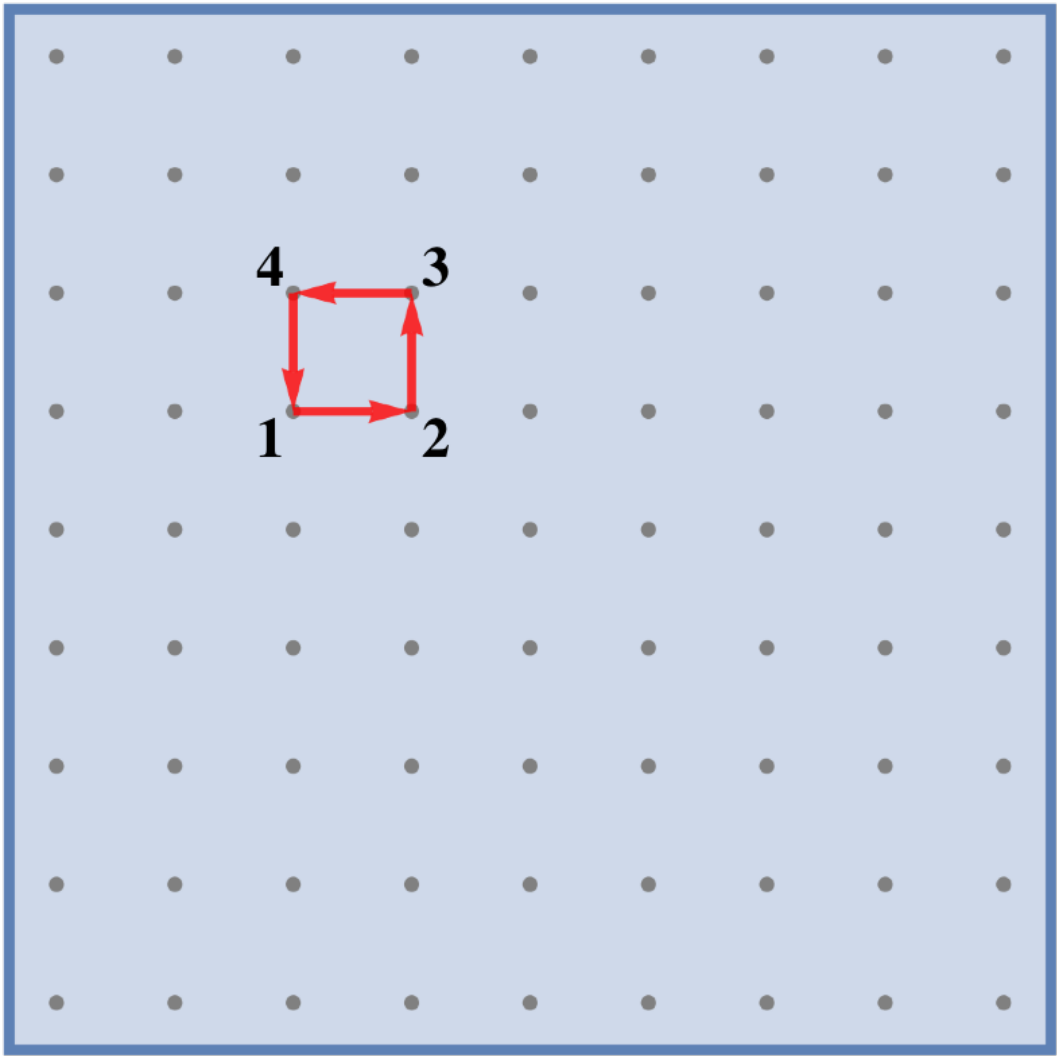
The continuous version of Chern number and Berry curvature is defined in Eq. (8) in the main text. To introduce the discrete version of Chern number, it is convenient to first define the Berry curvature in discrete spaces[62]. The Chern number is then the summation of Berry curvatures in the space.
The definition of the Berry curvature and the Chern number in discrete spaces, and the procedure for computing them are outlined as follows.
1. Discretize a two-dimensional parameter space as sites. With periodic boundary condition by identifying sites at the boundary, there are plaquettes in total. In our setting, sites are labeled as . For uniform discretization, the area of each plaquette is , where and is the distance of neighboring sites along and respectively.
2. At each site in the discretized two-dimensional parameter space, diagonalize the Hamiltonian to obtain the eigenstates of the -th band . is a diagonal matrix with its diagonal elements the eigenenergy of each band.
3. All four vertices in each plaquette construct an ordered loop, called the Wilson loop.
(a). Compute the ordered inner product of the eigenstates along the ordered loop in each plaquette. Specifically, define
(b). Define , where means to extract the diagonal elements and construct a diagonal matrix. That is, .
(c). Define . is the (non-Abelian) Berry curvature at the plaqutte labeled . Define and the Berry curvature of the -th band
| (10) |
4. The Chern number is the summation of the Berry curvature of all plaquettes. Define as the Chern number of the -th band:
| (11) |
It can be verified that the Chern number defined above is quantized and gauge invariant. For a model defined in the continuous space but whose Chern number is computed only on discretized points in the continuous space, Equation (11) gives the same result as Eq. (7) if the discretization is dense enough. Hence Eq. (10) and (11) can be seen as the generalization of the Berry curvature and the Chern number to discrete spaces.
References
- [1] LeCun, Yann, Yoshua Bengio, and Geoffrey Hinton. ”Deep learning.” nature 521.7553 (2015): 436.
- [2] Krizhevsky, Alex, Ilya Sutskever, and Geoffrey E. Hinton. ”Imagenet classification with deep convolutional neural networks.” Advances in neural information processing systems. 2012.
- [3] Farabet, Clement, et al. ”Learning hierarchical features for scene labeling.” IEEE transactions on pattern analysis and machine intelligence 35.8 (2013): 1915-1929.
- [4] Tompson, Jonathan J., et al. ”Joint training of a convolutional network and a graphical model for human pose estimation.” Advances in neural information processing systems. 2014.
- [5] Szegedy, Christian, et al. ”Going deeper with convolutions.” Cvpr, 2015.
- [6] Mikolov, Tomás̆, et al. ”Strategies for training large scale neural network language models.”Automatic Speech Recognition and Understanding (ASRU), 2011 IEEE Workshop on. IEEE, 2011.
- [7] Hinton, Geoffrey, et al. ”Deep neural networks for acoustic modeling in speech recognition: The shared views of four research groups.” IEEE Signal Processing Magazine 29.6 (2012): 82-97.
- [8] Sainath, Tara N., et al. ”Deep convolutional neural networks for LVCSR.” Acoustics, speech and signal processing (ICASSP), 2013 IEEE international conference on. IEEE, 2013.
- [9] Baldi, Pierre, Peter Sadowski, and Daniel Whiteson. ”Searching for exotic particles in high-energy physics with deep learning.” Nature communications 5 (2014): 4308.
- [10] Whiteson, Shimon, and Daniel Whiteson. ”Machine learning for event selection in high energy physics.” Engineering Applications of Artificial Intelligence 22.8 (2009): 1203-1217.
- [11] Ravanbakhsh, Siamak, et al. ”Enabling Dark Energy Science with Deep Generative Models of Galaxy Images.” AAAI. 2017.
- [12] Ball, Nicholas M., and Robert J. Brunner. ”Data mining and machine learning in astronomy.” International Journal of Modern Physics D 19.07 (2010): 1049-1106.
- [13] Al-Jarrah, Omar Y., et al. ”Efficient machine learning for big data: A review.” Big Data Research 2.3 (2015): 87-93.
- [14] Dieleman, Sander, Kyle W. Willett, and Joni Dambre. ”Rotation-invariant convolutional neural networks for galaxy morphology prediction.” Monthly notices of the royal astronomical society 450.2 (2015): 1441-1459.
- [15] Zhang, Pengfei, Huitao Shen, and Hui Zhai. ”Machine learning topological invariants with neural networks.” Physical review letters 120.6 (2018): 066401.
- [16] Morningstar, Alan, and Roger G. Melko. ”Deep learning the Ising model near criticality.” arXiv preprint arXiv:1708.04622 (2017).
- [17] Mano, Tomohiro, and Tomi Ohtsuki. ”Phase Diagrams of Three-Dimensional Anderson and Quantum Percolation Models Using Deep Three-Dimensional Convolutional Neural Network.” Journal of the Physical Society of Japan 86.11 (2017): 113704.
- [18] Rao, Wen-Jia, et al. ”Identifying product order with restricted Boltzmann machines.” Physical Review B 97.9 (2018): 094207.
- [19] Nomura, Yusuke, et al. ”Restricted Boltzmann machine learning for solving strongly correlated quantum systems.” Physical Review B 96.20 (2017): 205152.
- [20] Yoshioka, Nobuyuki, Yutaka Akagi, and Hosho Katsura. ”Machine Learning Disordered Topological Phases by Statistical Recovery of Symmetry.” Bulletin of the American Physical Society (2018).
- [21] Venderley, Jordan, Vedika Khemani, and Eun-Ah Kim. ”Machine learning out-of-equilibrium phases of matter.” arXiv preprint arXiv:1711.00020 (2017).
- [22] Suchsland, Philippe, and Stefan Wessel. ”Parameter diagnostics of phases and phase transition learning by neural networks.” arXiv preprint arXiv:1802.09876 (2018).
- [23] Arai, Shunta, Masayuki Ohzeki, and Kazuyuki Tanaka. ”Deep Neural Network Detects Quantum Phase Transition.” Journal of the Physical Society of Japan 87.3 (2018): 033001.
- [24] Li, Chian-De, Deng-Ruei Tan, and Fu-Jiun Jiang. ”Applications of neural networks to the studies of phase transitions of two-dimensional Potts models.”arXiv preprint arXiv:1703.02369 (2017).
- [25] Iakovlev, I. A., O. M. Sotnikov, and V. V. Mazurenko. ”Supervised learning magnetic skyrmion phases.” arXiv preprint arXiv:1803.06682 (2018).
- [26] Broecker, Peter, Fakher F. Assaad, and Simon Trebst. ”Quantum phase recognition via unsupervised machine learning.” arXiv preprint arXiv:1707.00663 (2017).
- [27] Carrasquilla, Juan, and Roger G. Melko. ”Machine learning phases of matter.” Nature Physics 13.5 (2017): 431.
- [28] Broecker, Peter, et al. ”Machine learning quantum phases of matter beyond the fermion sign problem.” Scientific reports 7.1 (2017): 8823.
- [29] Ch’ng, Kelvin, et al. ”Machine learning phases of strongly correlated fermions.” Physical Review X 7.3 (2017): 031038.
- [30] Zhang, Yi, and Eun-Ah Kim. ”Quantum loop topography for machine learning.” Physical review letters 118.21 (2017): 216401.
- [31] Zhang, Yi, Roger G. Melko, and Eun-Ah Kim. ”Machine learning Z 2 quantum spin liquids with quasiparticle statistics.” Physical Review B 96.24 (2017): 245119.
- [32] Ohtsuki, Tomoki, and Tomi Ohtsuki. ”Deep learning the quantum phase transitions in random two-dimensional electron systems.” Journal of the Physical Society of Japan 85.12 (2016): 123706.
- [33] Ohtsuki, Tomi, and Tomoki Ohtsuki. ”Deep learning the quantum phase transitions in random electron systems: Applications to three dimensions.” Journal of the Physical Society of Japan 86.4 (2017): 044708.
- [34] Schindler, Frank, Nicolas Regnault, and Titus Neupert. ”Probing many-body localization with neural networks.” Physical Review B 95.24 (2017): 245134.
- [35] Ponte, Pedro, and Roger G. Melko. ”Kernel methods for interpretable machine learning of order parameters.” Physical Review B 96.20 (2017): 205146.
- [36] Wang, Lei. ”Discovering phase transitions with unsupervised learning.” Physical Review B 94.19 (2016): 195105.
- [37] Tanaka, Akinori, and Akio Tomiya. ”Detection of phase transition via convolutional neural networks.” Journal of the Physical Society of Japan 86.6 (2017): 063001.
- [38] van Nieuwenburg, Evert PL, Ye-Hua Liu, and Sebastian D. Huber. ”Learning phase transitions by confusion.” Nature Physics 13.5 (2017): 435.
- [39] Liu, Ye-Hua, and Evert PL van Nieuwenburg. ”Discriminative Cooperative Networks for Detecting Phase Transitions.”Physical review letters 120.17 (2018): 176401.
- [40] Rui Li, Jiancheng Wang, Yiping Shu and Zhaoyi Xu. ”The discrepancy between Einstein mass and dynamical mass for SIS and power-law mass models.” arXiv preprint arXiv:1803.00819 (2018).
- [41] Wetzel, Sebastian J. ”Unsupervised learning of phase transitions: From principal component analysis to variational autoencoders.” Physical Review E 96.2 (2017): 022140.
- [42] Hu, Wenjian, Rajiv RP Singh, and Richard T. Scalettar. ”Discovering phases, phase transitions, and crossovers through unsupervised machine learning: A critical examination.” Physical Review E 95.6 (2017): 062122.
- [43] Costa, Natanael C., et al. ”Principal component analysis for fermionic critical points.” Physical Review B 96.19 (2017): 195138.
- [44] Wang, Ce, and Hui Zhai. ”Machine learning of frustrated classical spin models. I. Principal component analysis.” Physical Review B 96.14 (2017): 144432.
- [45] Ch’ng, Kelvin, Nick Vazquez, and Ehsan Khatami. ”Unsupervised machine learning account of magnetic transitions in the Hubbard model.” Physical Review E 97.1 (2018): 013306.
- [46] Huang, Li, and Lei Wang. ”Accelerated Monte Carlo simulations with restricted Boltzmann machines.” Physical Review B 95.3 (2017): 035105.
- [47] Huang, Li, Yi-feng Yang, and Lei Wang. ”Recommender engine for continuous-time quantum Monte Carlo methods.” Physical Review E 95.3 (2017): 031301.
- [48] Liu, Junwei, et al. ”Self-learning monte carlo method.” Physical Review B 95.4 (2017): 041101.
- [49] Liu, Junwei, et al. ”Self-learning Monte Carlo method and cumulative update in fermion systems.” Physical Review B 95.24 (2017): 241104.
- [50] Nagai, Yuki, et al. ”Self-learning Monte Carlo method: Continuous-time algorithm.” Physical Review B 96.16 (2017): 161102.
- [51] Xu, Xiao Yan, et al. ”Self-learning quantum Monte Carlo method in interacting fermion systems.” Physical Review B 96.4 (2017): 041119.
- [52] Shen, Huitao, Junwei Liu, and Liang Fu. ”Self-learning Monte Carlo with Deep Neural Networks.” arXiv preprint arXiv:1801.01127 (2018).
- [53] Arsenault, Louis-François, et al. ”Machine learning for many-body physics: the case of the Anderson impurity model.” Physical Review B 90.15 (2014): 155136.
- [54] Arsenault, Louis-François, O. Anatole von Lilienfeld, and Andrew J. Millis. ”Machine learning for many-body physics: efficient solution of dynamical mean-field theory.” arXiv preprint arXiv:1506.08858 (2015).
- [55] Deng, Dong-Ling, Xiaopeng Li, and S. Das Sarma. ”Quantum entanglement in neural network states.” Physical Review X 7.2 (2017): 021021.
- [56] Lu, Sirui, et al. ”A Separability-Entanglement Classifier via Machine Learning.” arXiv preprint arXiv:1705.01523 (2017).
- [57] Levine, Yoav, et al. ”Deep learning and quantum entanglement: Fundamental connections with implications to network design.” CoRR, abs/1704.01552 (2017).
- [58] You, Yi-Zhuang, Zhao Yang, and Xiao-Liang Qi. ”Machine learning spatial geometry from entanglement features.” Physical Review B 97.4 (2018): 045153.
- [59] This is to be compared with a fully-connected neural network without this symmetry constraint, which may contain more parameters but is more difficult to be trained to the optimal solution that reproduces the translational symmetry [15].
- [60] Here we assume is a square matrix for simplicity [61]. Although in general might not be unitary, we can always make the flat-band approximation for a gapped system such that the topological property remains invariant. The matrix is then unitary and takes the form of Eq. (1).
- [61] Chiu, Ching-Kai, et al. ”Classification of topological quantum matter with symmetries.” Reviews of Modern Physics 88.3 (2016): 035005.
- [62] Fukui, Takahiro, Yasuhiro Hatsugai, and Hiroshi Suzuki. ”Chern numbers in discretized Brillouin zone: efficient method of computing (spin) Hall conductances.”Journal of the Physical Society of Japan 74.6 (2005): 1674-1677.