Symmetric and asymmetric discrimination of bosonic loss:
Toy applications to biological samples and photo-degradable materials
Abstract
We consider quantum discrimination of bosonic loss based on both symmetric and asymmetric hypothesis testing. In both approaches, an entangled resource is able to outperform any classical strategy based on coherent-state transmitters in the regime of low photon numbers. In the symmetric case, we then consider the low-energy detection of bacterial growth in culture media. Assuming an exponential growth law for the bacterial concentration and the Beer-Lambert law for the optical transmissivity of the sample, we find that the use of entanglement allows one to achieve a much faster detection of growth with respect to the use of coherent states. This performance is also studied by assuming an exponential photo-degradable model, where the concentration is reduced by increasing the number of photons irradiated over the sample. This investigation is then extended to the readout of classical information from suitably-designed photo-degradable optical memories.
I Introduction
Today we use classical or semi-classical sources of radiation for a plethora of practical applications. A natural question to ask is how far we can improve these applications by resorting to the laws of quantum mechanics and the new framework of quantum information [1, 2, 3, 4, 5, 6, 7, 8]. In fact, nonclassical states represent a completely new resource for future quantum technology, once their generation and manipulation becomes routinely possible outside quantum labs. Examples of nonclassical states are number states, squeezed states and entangled states. In particular, quantum entanglement is one of the key properties exploited in many quantum information tasks, e.g., in protocols of quantum teleportation [9, 10, 11], quantum metrology [12, 13, 14, 15, 16, 17], and quantum cryptography [18]. In the bosonic case, entanglement is usually present in the form of Einstein-Podolsky-Rosen (EPR) correlations [19], where the quadrature operators of two bosonic modes are so correlated to beat any possible classical description.
Entanglement and, more generally, quantum correlations have already led to non-trivial improvements in information tasks that are based on quantum hypothesis testing [20, 21, 22, 23, 24, 25, 26, 27, 28], such as the detection of targets or quantum illumination [29, 30, 31, 32, 33, 34, 35, 36, 37], and the readout of digital optical memories or quantum reading [38, 39, 40, 41, 42, 43, 44, 45, 46, 47, 48, 49, 50, 51]. These enhancements are particularly evident when the number of photons involved in the process is relatively low. A very important scenario where low energy matters is in the context of fragile material in biological samples. In this case, faint quantum light may effectively probe the material without destroying it.
In this paper, we consider this context. We study the detection of bosonic loss in fragile photo-degradable materials. First, we review the theory of quantum discrimination of bosonic loss by extending previous results from symmetric to asymmetric hypothesis testing. Then, we show how quantum entanglement can effectively be used to discriminate the presence or absence of bacterial growth in a biological sample. The advantage is quantified in terms of speed of detection with respect to the use of a coherent-state transmitter under the same (relatively-low) number of mean photons irradiated over the sample. We show energy regimes where this advantage becomes non-trivial, and how it can also be used to build fragile memories where information remains hidden to standard optical readers (extending previous ideas from Ref. [50]).
The manuscript is structured as follows. In Sec. II we provide a brief review of quantum hypothesis testing considering its symmetric and asymmetric formulation. In Sec. III, we consider the quantum discrimination of bosonic loss and its connection with the detection of non-zero concentration in samples. In Sec. IV, we discuss the classical benchmark associated with coherent-state transmitters. While this is known for symmetric testing, here we also provide its expression for the asymmetric case. In Sec. V, we then consider the entanglement-based quantum transmitter, providing its performance for both symmetric and asymmetric testing. In Sec. VI, we explicitly compare classical and quantum transmitters under the two different types of testing, and consider single- and multi-copy (asymptotic) discrimination. In Sec. VII we apply the tools to bacterial growth in a sample assuming an exponential growth model and a toy model of photo-degradability. In Sec. VIII, we extend the treatment to digital memories. Finally, Sec. IX is for conclusions.
II Quantum hypothesis testing
II.1 Bayesian cost
We start by providing a brief survey of the concept of Bayesian cost and its connection with symmetric and asymmetric hypothesis testing. For simplicity, we consider the specific case of a binary hypothesis test, but the notion can easily be generalized and formulated for different hypotheses.
Let us consider a binary test with hypotheses (null) and (alternate), occurring with some a priori probabilities and , respectively. In the quantum setting, these hypotheses are associated with two possible states, and , taken by some quantum system, i.e., we may write
| (1) | ||||
| (2) |
Associated with the test, there is the conditional probability of choosing the hypothesis when the actual hypothesis is , with . In a quantum test, this probability is determined by the quantum measurement which is performed on the system. In particular, it is always sufficient to consider a dichotomic quantum measurement, described by a positive operator-valued measure (POVM) with two operators and . Thus, we may write the Born rule
| (3) |
For , we have error probabilities, known as false-negative probability , and false-positive probability . In general, we can also introduce a cost matrix , whose generic element represents the ‘cost’ associated with conditional probability . Thus, the goal of the binary test is to minimize the following Bayes’ cost function
| (4) |
In particular, we may choose
| (5) |
so that
| (6) |
Depending on the choice of and , we may have a symmetric or asymmetric hypothesis test. When the costs are the same (), we retrieve symmetric hypothesis testing. Here the cost function simply becomes the mean error probability of the test
| (7) |
By contrast, in case of completely unbalanced costs, such as or , we have asymmetric hypothesis testing, with the cost function collapsing into the false-negative error probability, i.e., .
II.2 Symmetric Testing
Here we describe the main tools used in the symmetric testing of two quantum hypotheses, considering (for simplicity) the case of a uniform a priori probability distribution . The mean error probability associated with the test is minimized by the Helstrom POVM [20] and is given by the Helstrom bound
| (8) |
where is the trace distance between the two quantum states [1, 2].
In general, the two states can be a tensor product of single-copy states, i.e.,
| (9) |
In this multi-copy discrimination setting, a very useful tool is the quantum Chernoff bound (QCB) [52, 53, 54]. This is an upper-bound , which is defined as
| (10) |
where is the -overlap between the two single-copy states and . The QCB is asymptotically tight, meaning that we have for [52, 53].
II.3 Asymmetric Testing
In the regime of many copies , we can write the following asymptotic behaviors for the error probabilities associated with the test
| (14) | ||||
| (15) |
where is the error-rate exponent of the false-positive probability, and is the error-rate exponent of the false-negative probability.
In asymmetric quantum discrimination, we aim to maximize the error-rate exponent of the false negatives while constraining the error-rate exponent of the false positives with a positive parameter . By optimizing over all the possible quantum measurements , the maximum error-rate is given by the quantum Hoeffding bound (QHB) [59], which is defined as
| (16) |
In case of Gaussian states and , the QHB can be computed from their statistical moments [60] (see Appendix A).
II.4 Discriminating a pure state from a mixed state
In the specific case where one of the two states is pure, say , we have some simplifications in the above tools. First of all, the QCB can be directly computed from the quantum fidelity as
| (17) |
so that we can write
| (18) |
Then, the QHB satisfies the inequality
| (19) |
As a result, we may write
| (20) |
This is intuitively expected because it is surely easier to minimize the false-negative error probability , constraining the false positive error probability , rather than minimizing their average . However, if the control on the false-positives is good, here meaning that , then the QHB and the QCB coincides. In fact, we have
| (21) |
which clearly implies .
The proof of Eqs. (19) and (21) is easy. First, from the definition of the QHB, we note that we can generally write the inequality
| (22) | ||||
| (23) |
Now, if , then we have [58]
| (24) |
which provides Eq. (19). Furthermore, in this case of one pure state, Ref. [60] proved the following upper-bound
| (25) |
By combining Eq. (19) and (25), we then derive the result of Eq. (21).
II.5 Discriminating two pure states
In the stronger case where both the states are pure, i.e., and , we have further simplifications. For the multi-copy Helstrom bound, we can write
| (26) |
where the trace distance can be here computed from the fidelity as
| (27) | ||||
| (28) |
where
| (29) |
III Quantum discrimination of Loss
The above tools of quantum hypothesis testing can also be employed to solve problems of quantum channel discrimination. Here, an unknown quantum channel, or , is prepared inside an input-output black-box and passed to a reader [5, Sec. V.H], whose aim is to distinguish the two channels by probing the input port and measuring the output. In the bosonic setting, this problem can be further constrained by considering Gaussian channels [5], in particular, lossy channels which are characterized by a single transmissivity parameter . These channels can be dilated into beam-splitters subject to vacuum noise (see Appendix B for more details on lossy channels).
In this paper we are interested in sensing the presence of loss, which corresponds to the discrimination between a lossless channel (i.e., the identity channel ) from a lossy channel with some transmissivity . In other words, we consider transmissivity as our null hypothesis , and transmissivity as our alternative hypothesis .
This problem is relevant in biological problems, such as the detection of small concentrations of cells or bacteria. The connection is established by the Beer-Lambert law [61]. Accordingly to this law, the concentration of species within a sample can be connected with its absorbance or transmissivity by the formula
| (31) |
where is an absorption coefficient (for that species), and is the path length. From an optical point of view, the sample is therefore equivalent to a lossy channel with concentration-dependent transmissivity . Our problem can be mapped into the discrimination between non-growth and growth within a biological sample.
An important issue is related with the amount of energy employed to probe the black-box or, equivalently, the sample in the biological setting just described. First of all, a problem of Gaussian channel discrimination makes sense only if we assume an energetic constraint for the optical mode probing the box, otherwise any two different channels can always be perfectly distinguished (using infinite energy).
Second, we assume that this constraint imposes an effective regime of few photons, so that the box is read in a noninvasive way, which fully preserves its content. This is particularly important from a biological point of view, since bacteria may be photo-degradable and DNA/RNA extracts in samples can easily be degraded by strong light (especially, in the UV regime).
Thus, in our quantum sensing of loss, we assume suitable energetic constraints at the input, which may be of two kinds:
- (1)
-
Local energetic constraint, where we fix the mean number of photons employed in each single readout of the box; in particular, we are interested in the use of a single readout and in the limit of many readouts (e.g., using a broadband signal).
- (2)
-
Global energetic constraint, where we fix the mean number of photons which are used in totality, i.e., over all the readouts of the box.
Imposing one of these constraints and a suitable regime of few photons, our work aims to prove the superiority of quantum-correlated sources with respect to classical sources for noninvasive sensing of loss.
As shown by the setups of Fig. 1, we first consider a classical strategy where a single-mode , prepared in a classical state (in particular, a coherent state), is irradiated through the sample and detected at the output by an optimal dichotomic POVM. Then, we compare this approach with the quantum strategy where two modes, signal and reference , are prepared in a quantum correlated state, in particular, a two-mode squeezed vacuum (TMSV) state, which is a finite-energy version of an Einstein-Podolsky-Rosen (EPR) state [5]. Only the signal mode is irradiated through the sample, while the reference mode is directly sent to the measurement setup where it is subject to an optimal dichotomic POVM jointly with the output mode from the sample.
The readout performance of these two setups are compared by constraining the energy of the signal mode , by fixing the mean number of photon per mode (local constraint), or the total mean number of photons in probings of the sample. The performance is evaluated in terms of minimum error probability considering both symmetric and asymmetric hypothesis testing.
IV Classical Benchmark
In the classical setup of Fig. 1(a), the input signal mode is prepared in a coherent state and transmitted through the sample. At the output, the receiver may be a photon counting detector, which is then followed by post-processing of the outcomes. The performance of this receiver can always be bounded by considering an optimal dichotomic POVM (e.g., the Helstrom POVM [20] in symmetric testing and other suitable dichotomic POVMs in the asymmetric case [59]).
Let us solve this problem in the general multi-copy scenario, where the sample is probed times, so that the input state is given by the tensor product
| (32) |
It is clear that the output states will be either (under hypothesis ) or (under hypothesis ).
Since the two possible outputs are pure states, we can easily compute the Helstrom bound (for symmetric testing) and the QHB (for asymmetric testing) according to Sec. II.5. In fact, we just need to compute the fidelity between the single-copy output states
| (33) | ||||
| (34) |
where is the mean number of photons of the single-copy coherent state at the input.
Then, using Eqs. (26)-(28), one derives the following Helstrom bound for the coherent-state transmitter [38]
| (35) |
We can see that the minimum error probability depends on the total mean number of photons . This means that it makes no difference to use: (i) either identical faint coherent states each with mean photons, (ii) or a single energetic coherent state with mean photons. Also note that, for , we have , i.e., random guessing. Discrimination becomes therefore challenging at low photon numbers.
Note that it is also easy to compute the QCB. Since the two states are pure, we can write it in terms of the quantum fidelity as specified by Eq. (18), which here becomes
| (36) |
One can easily check that this is an upper-bound to the minimum error probability of Eq. (35), becoming tight in the limit of a large number of copies .
In the case of asymmetric quantum discrimination, we aim to minimize the probability of false negatives . In a biological sample, this means one should minimize the probability of concluding that there is no growth of bacteria when there actually is. More precisely, we aim to derive the QHB which maximizes the error-rate exponent of in the regime of many copies , while constraining the error-rate exponent for the false positives . By using Eq. (30), we derive
| (37) |
Here we note that for bad control of the false positives , the QHB has a super-exponential decay in . In contrast, for good control of the false positives , the QHB has the following asymptotic exponential decay
| (38) | ||||
| (39) |
which is the same as the QCB in Eq. (36). This an intuitive result because in the case of good control, besides Eq. (39), we also have
| (40) | ||||
| (41) |
Thus, by replacing Eqs. (39) and (41) in the average error probability of Eq. (7), we retrieve
| (42) |
V Quantum Transmitter
In the quantum setup of Fig. 1(b), we consider a transmitter composed of two quantum-correlated modes, the signal and the reference . The signal mode, with mean photons, is irradiated through the sample and its output is combined with the reference mode in an optimal quantum measurement. For a fixed state of the input modes and , we get two possible states
| (43) | ||||
| (44) |
for the output modes and at the receiver. In general, for multi-copy discrimination, the input tensor product is transformed into either or .
As an example of a single-copy state let us consider a TMSV state (or realistic EPR source). This is a zero-mean pure Gaussian state with covariance matrix (CM) [5]
| (45) |
where quantifies both the mean number of thermal photons in each mode, given by , and the amount of signal-reference entanglement [5].
Using such a state at the input, we get two possible zero-mean Gaussian states at the output: One is just the input TMSV state , while the other state is mixed and has CM (see Appendix C)
| (46) |
Since one of the output states is pure, we can exploit the tools of Sec. II.4.
For symmetric testing we compute the QCB, which can be directly derived from the quantum fidelity, as specified in Eq. (18). The multi-copy minimum error probability is upper-bounded by
| (47) |
where the fidelity is determined by the CMs of the two Gaussian states [58]. This is equal to
| (48) |
Thus, we have [38]
| (49) |
For asymmetric testing we compute the QHB. From Eq. (19), we may write
| (50) |
More precisely, according to Eq. (21), we have
| (51) |
for . Then, we have numerically checked that for , the QHB can become infinite. This can be checked by computing the QHB directly from Eq. (16) and using the Gaussian formula for the -overlap (see Appendix D for more details).
VI Comparison and Quantum Advantage
In this section, we compare the classical and quantum strategies for noninvasive sensing of loss, showing how the use of quantum correlations enables us to outperform the classical benchmark achieved with coherent-state inputs. For symmetric testing, we consider the difference (or gain)
| (52) |
using the expressions in Eqs. (35) and (49). Its positivity is a sufficient condition for the superiority of the quantum transmitter (while corresponds to an inconclusive comparison). In particular, for close to , we have that and , which means that the quantum strategy allows for perfect sensing while the classical strategy is equivalent to random guessing.
We start by considering a single probing of the sample, i.e., . Then, we plot considering the regime of small photon numbers () and for . As we can see from Fig. 2, the quantum transmitter is better in most of the parameter plane, with very good performances for close to (which corresponds to sensing an almost transparent growth). To better explore this region we consider the expansion for . By setting , we get the first-order expansion
| (53) |
so that
| (54) |
which is always positive.
We then analyze the multi-probing case where the samples are queried times where we fix the mean number of photons per signal mode (local energy constraint). We then specify the gain for , and we plot the results in Fig. 3. We see that the good region where approaches the optimal value of is again for transmissivities .
VI.1 Asymptotic multi-copy behavior
Here we keep the local energy constraint, i.e., we fix the mean number of photons per signal mode , and we compare the two transmitters in the limit of a large number of copies . In this limit the mean error probability in the symmetric test is well approximated by the QCB, so that, from Eqs. (36) and (49), we can write
| (55) |
where , and
| (56) |
where . Thus, the asymptotic gain can be measured by the ratio
| (57) |
It is clear that for , the error probability of the EPR transmitter goes to zero more rapidly than that of the coherent-state transmitter (while corresponds to the opposite behavior). This ratio is shown in Fig. 4. We see that for high values of the transmissivity, the EPR transmitter has an error exponent which becomes orders of magnitude higher than the classical one .
VI.2 Asymptotic multi-copy behavior: Asymmetric testing
Assuming a local energy constraint we now compare the quantum and the classical coherent transmitter from the point of view of asymmetric testing. We consider the ratio between the two QHBs, i.e., for any control we define
| (58) |
According to Eqs. (37) and (50), we have
| (59) |
and
| (60) |
where
| (61) |
If we assume good control on the false positives, i.e., , then we find that the false negative probability is well approximated by the QCB, i.e., (see Sec. II.4). As a result, the ratio in Eq. (58) asymptotically coincides with the previous ratio in Eq. (57), i.e., , and the same result shown in Fig. 4 also applies to asymmetric testing.
Let us now study what happens in the presence of moderate control of false positives. Let us consider the case which happens in a delimited region of the plane corresponding to the non-black area in Fig. 5. Then, we assume , so that remains finite, while can become infinite. As we see from Fig. 5, there is a wide area where , meaning that the quantum EPR transmitter provides a super-exponential decay for the false-negative probability, while it remains exponential for the classical transmitter.
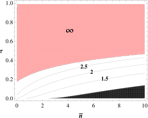
If we consider the opposite case , which may only occur in the black area of Fig. 5, then we see that becomes infinite while remains finite. In other words, we have in all the black region. Finally, for there are indeterminate forms which do not allow us to provide a simple description of the situation.
From these results it is clear that, for low photon numbers per mode () and high transmissivities (here ), the quantum EPR transmitter greatly outperforms the classical transmitter in the asymmetric quantum discrimination of loss.
VI.3 Comparison under the global energy constraint
In order to study the case of the global constraint we set in the QCB in Eq. (49), so that it can expressed as . As we show in Fig. 6, the value of decreases for increasing , at fixed total energy and transmissivity . In other words, it is better to use a large number of copies () of the TMSV state with vanishingly small number of photons per copy (), instead of a single energetic TMSV state with mean photons . Remarkably the asymptotic behavior is rapidly reached after a finite number of copies, e.g., for .
For large , we find the optimal asymptotic expression
| (62) |
and we find the optimal gain is
| (63) |
As shown in Fig. 7, we can see that for relatively small numbers of photons , globally irradiated over the sample the EPR transmitter clearly outperforms the classical strategy, especially for high transmissivities . In other words, the use of a quantum source has non-trivial advantages for the noninvasive detection of small concentrations. Luckily, we do not have to consider the limit of for approaching the optimal performance of the EPR transmitter since, as we have already seen in Fig. 6, this performance is approximately reached with small finite . Indeed, we have numerically checked that already provides a good approximation of the asymptotic behavior.
VII Biological growth and photodegradability
VII.1 Non-invasive detection of growth in biological samples
As discussed in Sec. III, the concentration of species within a sample can be connected with its transmissivity by the formula , where is an absorption coefficient and is the path length. Thus, the sample is a lossy channel with concentration-dependent transmissivity and the problem of loss detection can be mapped into the discrimination between non-growth and growth within the sample. For simplicity, in the following we set , so that .
We then introduce a phenomenological model of bacterial/cell growth in the sample, so that the concentration depends on time (abstract units) in a typical exponential law
| (64) |
where is a saturation parameter and is the asymptotic concentration (at infinite time). Using Eq. (64) we can write as a function of time as follows
| (65) |
Now we can analyze how well we can distinguish between unit transmissivity (no growth) and (growth) at any specified time . For this aim, we replace in the error probabilities associated with the classical and quantum EPR transmitter. We consider the case of symmetric testing and we assume a global energy constraint so that we fix the mean total number of photons irradiated over the sample.
Mathematically, we then plug into the formula of of Eq. (35) for the classical transmitter, so that we can write . Similarly, for the quantum EPR transmitter, we plug into the formula of of Eq. (49) where . In this case, we can write and study the two extreme conditions of a single-mode EPR transmitter () and the broadband EPR transmitter with (any other EPR transmitter with arbitrary will have a performance between these two extremes).
As before we can make the comparison by using the gain whose maximal value is . Specifically, we consider the gain given by the single mode EPR transmitter
| (66) |
and the optimal gain given by the broadband EPR transmitter, i.e.,
| (67) |
We compare the performances of the classical and quantum transmitters plotting and in Fig. 8.
As we can see from Fig. 8, the EPR transmitter outperforms the classical strategy at short times, i.e., at low concentrations, when the mean total number of photons is restricted to relatively small values. This means that, in this non-destructive regime, the EPR transmitter is able to provide a much faster detection of bacterial/cell growth in the sample. This is also evident from Fig. 9, where we explicitly compare the performances of the transmitters at photons. As we can see, the quantum transmitter allows us to detect the presence or absence of a growth in extremely short times ( time units in the figure), while we need to wait longer times (at least time units) for obtaining the same performance by means of a classical transmitter.
VII.2 Model combining growth and photo-degradability
We now combine the previous exponential growth model with a model of photo-degradability. We assume that the concentration decays for increasing photon number . More precisely, we assume that the concentration decay by a factor where is a degradability parameter, is the mean number of photons irradiated over the sample (constantly per unit of time), and is the time of the readout. We assume that at time the sample has been already irradiated with mean photons, and the duration of the readout is equal to one time unit. Combining this process with the growth model, we have
| (68) |
and a corresponding model for the transmissivity according to the Beer-Lambert law.
For simplicity, here we set , , and . In Fig. 10 we show the behavior of the concentration versus time and the corresponding performances of the quantum and classical transmitters. The plot shows that the quantum transmitter clearly outperforms the classical benchmark in terms of fast detection times. As a matter of fact, in the regime of parameters investigated, the growth is present only in a small time window (before the sample is degraded). Within this window, the quantum transmitter is able to detect bacterial growth with certainty, while the classical transmitter has a non-trivial error probability ().
VIII Fragile data storage
A practical scenario where the quantum detection of loss is important is that of quantum reading [38], where the aim is to boost the retrieval of classical data from an optical disk by exploiting quantum entanglement at low photon numbers. A basic setup for quantum reading consists of a series of cells, each one encoding a bit of information. This is physically done by picking two different reflectivities, and , each encoding a different bit value. A target cell is then read by shining optical modes on it (generated by the transmitter) and detecting their reflection back to a receiver. The use of an entangled source is known to retrieve more information than any classical source (e.g., based on a mixture of coherent states).
Here we consider the same basic model but in transmission, i.e., assuming that the bit-values are encoded in two different transmissivities, and , and with the cells positioned between the transmitter and the receiver. This is completely equivalent from a mathematical point of view (since ). Similarly to Ref. [50], we show that the advantage given by a quantum EPR transmitter can be made extreme by introducing a suitable photodegradable model for the memory. In fact, we can assume a specific saturation behavior for the memory cells in such a way that their transmissivities tend to coincide if we increase the amount of energy adopted for their readout. Assuming this model, we find wide regions of parameters where the EPR transmitter is able to retrieve the maximum value of bit per cell, while the classical coherent transmitter decodes bits per cell. As we discuss below, this striking difference can be exploited as a cryptographic technique.
As before we assume that and . We can introduce a simple saturation effect by imposing that the lower transmissivity tends to for increasing photon numbers. This may be realized by imposing the exponential law
| (69) |
where is the mean total number of photons employed in each probing, while and are parameters of the phenomenological model. More specifically, parameter provides the value at zero energy (which is ), and parameter gives the speed of convergence to .
In order to evaluate the effects of this saturation behavior, we have to combine the law of Eq. (69) with the energy-dependent performances of the quantum and classical transmitters. First of all, since we are considering the readout of a memory cell, we connect the error probability in the channel discrimination with the amount of information retrieved . This connection is given by the formula
| (70) |
where is the binary Shannon entropy. Thus, for the coherent transmitter, we have where is given in Eq. (35). For the quantum EPR transmitter, we have , where the QCB is given in Eq. (49) and . Thus, for any fixed choice of the parameters and , we can replace in the previous information quantities, so to have and .
At fixed values of the energy , we then compare the number of bits retrieved by the classical transmitter with those retrieved by the quantum EPR transmitter for (i.e., a single energetic mode with mean photons) and for (i.e., an infinite number of modes with vanishing mean photons ). The performance of the quantum transmitter for arbitrary will be bounded by these two extremal curves. This comparison is shown in Fig. 11 where we assume several values for the parameters and . From the previous figure it is clear that we can consider photodegradable models such that the classical transmitter is not able to retrieve any information, while the EPR transmitter can retrieve almost all the information in a specific range of energies, depending on the ’s.
This extreme situation could be exploited for cryptographic tasks. In particular, an optical memory could be purposely constructed to be photo-degradable in such a way as to hide its encoded classical data from any standard optical drives based on the use of coherent (or thermal) light. Only an advanced laboratory able to engineer a quantum entangled source in the correct window of energy will be able to read out the stored confidential data. From this point of view, quantum reading can provide a potential technological layer of security based on the fact that the generation of entanglement and other non-classical features is only possible in more advanced labs of quantum optics. Furthermore, the range of energy to be used must also be very well-tailored depending on the specific parameters and employed during data storage which means that even an eavesdropper with an advanced laboratory is likely to destroy the data. These concepts are clearly preliminary but the basic ideas could further be developed into potential practical applications.
IX Conclusions
Partly building on previous analyses (e.g., Ref. [38]), we have considered the quantum discrimination of bosonic loss and extended results from symmetric to asymmetric testing. In particular, we have derived the quantum Hoeffding bound associated with the discrimination of loss by means of coherent states (classical benchmark/transmitter) and TMSV states (quantum EPR transmitter). Then, we have applied symmetric testing to the study of fragile systems. In fact, we have shown how the use of quantum entanglement greatly outperforms classical strategies (based on coherent-state transmitters) for the low-energy detection of small concentrations in samples. Assuming models of bacterial growth and photo-degradability, we have shown parameter regimes where quantum entanglement guarantees a very fast detection of growth, while coherent-state transmitters are very slow or even unable to detect the presence of bacteria.
Similar results are shown for the readout of photo-degradable optical memories. Future steps involve the study of the quantum advantage by considering other phenomenological models of bacterial growth and photo-degradability. In the long run, these principles can be exploited to design more advanced types of biological instrumentations, such as noninvasive quantum-enhanced spectrophotometers for concentration detection and measurement. Because of the absence of degradation, fragile samples could also be re-used or continuously probed in a real-time fashion.
X Acknowledgments
This work has been sponsored by the European Commission under the Marie Sklodowska-Curie Fellowship Progamme (EC grant agreement No 745727), the EPSRC and the Leverhulme Trust (‘qBIO’ fellowship). G.S. would like to thank Seth Lloyd for feedback.
Appendix A Formulas for Gaussian states
For the sake of completeness we provide the formula for the -overlap between two Gaussian states, originally proven in Ref. [54]. This formula enables us to compute the QCB in Eq. (10) and the QHB in Eq. (16). Here we specify this formula for the case of two-mode Gaussian states.
Given a pair of two-mode Gaussian states and , their -overlap can be computed in terms of their first- and second-order statistical moments, i.e., their mean values, and , and their CMs, and . In particular, the CMs can be decomposed as
where and are their symplectic spectra, and and are symplectic matrices [5].
Let us introduce the following real functions depending on the parameter
| (75) | ||||
| (76) |
Then, the -overlap can be written as
| (77) |
where ,
| (78) |
and
Appendix B Single-mode Gaussian channels and lossy channels
Let us consider a single bosonic mode in a Gaussian state , with mean value and covariance matrix (CM) . The action of a Gaussian channel on this state can be easily expressed in terms of simple transformations on its statistical moments. In particular, we have [5]
| (87) | ||||
| (88) |
where is a displacement vector, a transmission matrix, and a noise matrix (satisfying suitable bona-fide conditions [5]).
Appendix C Computation of the CM in Eq. (46)
To compute the CM of the output state , we dilate the lossy channel into a beam splitter (with transmissivity ), mixing the signal mode with a vacuum mode . Thus, we have a Gaussian unitary transformation from the input state of modes into the output state of modes , i.e.,
| (90) |
where is the beam-splitter unitary [5] applied to modes and , while the reference mode is subject to the identity. In terms of CMs, we have
| (91) |
where and
| (92) |
is the symplectic transformation of the beam splitter. After simple algebra, we find an output CM of the form
| (93) |
where the blocks and are to be traced out, while is given in Eq. (46).
Appendix D QHB for the quantum transmitter
Here we compute the QHB for the quantum EPR transmitter directly from the Gaussian formula for the -overlap given in Appendix. A. Since the two output states generated by the EPR transmitter are zero-mean, we can write the -overlap as
| (94) |
To compute and , we note that describes a pure state, which means that its symplectic spectrum is trivial and . Since , we may write
| (95) |
and
| (96) |
References
- [1] J. Watrous, The theory of quantum information (Cambridge University Press, Cambridge, 2018). Also available from https://cs.uwaterloo.ca/˜watrous/TQI/TQI.pdf
- [2] M. Hayashi, Quantum Information Theory: Mathematical Foundation (Springer-Verlag Berlin Heidelberg, 2017).
- [3] M. A. Nielsen, and I. L. Chuang, Quantum computation and quantum information (Cambridge University Press, Cambridge, 2000).
- [4] S. L. Braunstein, and P. Van Loock, Rev. Mod. Phys. 77, 513 (2005).
- [5] C. Weedbrook et al., Rev. Mod. Phys. 84, 621 (2012).
- [6] G. Adesso, S. Ragy, and A. R. Lee, Open Syst. Inf. Dyn. 21, 1440001 (2014).
- [7] A. Serafini, Quantum Continuous Variables: A Primer of Theoretical Methods (Taylor & Francis, Oxford, 2017).
- [8] U. L. Andersen, J. S. Neergaard-Nielsen, P. van Loock, and A. Furusawa, Nat. Phys. 11, 713–719 (2015).
- [9] C. H. Bennett, G. Brassard, C. Crepeau, R. Jozsa, A. Peres, and W. K. Wootters, Phys. Rev. Lett. 70, 1895 (1993).
- [10] S. L. Braunstein and H. J. Kimble, Phys. Rev. Lett. 80, 869–872 (1998).
- [11] S. Pirandola et al., Nat. Photon. 9, 641–652 (2015).
- [12] S. L. Braunstein, and C. M. Caves, Phys. Rev. Lett. 72, 3439 (1994).
- [13] C. M. Caves, and G. J. Milburn, Ann. Phys. 247, 135 (1996).
- [14] M. G. A. Paris, Int. J. Quant. Inf. 7, 125-137 (2009).
- [15] V. Giovannetti, S. Lloyd, and L. Maccone, Nature Photon. 5, 222 (2011).
- [16] R. Laurenza, C. Lupo, G. Spedalieri, S. L. Braunstein, and S. Pirandola, Quantum Meas. Quantum Metrol. 5, 1-12 (2018).
- [17] D. Braun et al., Rev. Mod. Phys. 90, 035006 (2018).
- [18] A. K. Ekert, Phys. Rev. Lett. 67, 661–663 (1991).
- [19] A. Einstein, B. Podolsky, and N. Rosen, Phys. Rev. 47, 777 (1935).
- [20] C. W. Helstrom, Quantum Detection and Estimation Theory (New York: Academic, 1976).
- [21] A. Chefles, Contemp. Phys. 41, 401 (2000).
- [22] S. M. Barnett and S. Croke, Adv. Opt. Photon. 1, 238-278 (2009).
- [23] J. A. Bergou, U. Herzog, and M. Hillery, Discrimination of Quantum States, in Quantum state estimation, Lecture Notes in Physics, Springer-Verlag Berlin Heidelberg (2004), pp 417-465.
- [24] Y. Sun, J. A. Bergou, and M. Hillery, Phys. Rev. A 66, 032315 (2002).
- [25] J. A. Bergou, and M. Hillery, Phys. Rev. Lett. 94, 160501 (2005).
- [26] J. A. Bergou, V. Bužek, E. Feldman, U. Herzog, and M. Hillery, Phys. Rev. A 73, 062334 (2006).
- [27] J. A. Bergou, E. Feldman, and M. Hillery, Phys. Rev. A 73, 032107 (2006).
- [28] C. Invernizzi, M. G.A. Paris, and S Pirandola, Phys. Rev. A 84, 022334 (2011).
- [29] S. Lloyd, Science 321, 1463 (2008).
- [30] S.-H. Tan, B. I. Erkmen, V. Giovannetti, S. Guha, S. Lloyd, L. Maccone, S. Pirandola, and J. H. Shapiro, Phys. Rev. Lett. 101, 253601 (2008).
- [31] J. H. Shapiro, and S. Lloyd, New J. Phys. 11, 063045 (2009).
- [32] S. Barzanjeh, S. Guha, C. Weedbrook, D. Vitali, J. H. Shapiro, and S. Pirandola, Phys. Rev. Lett. 114, 080503 (2015).
- [33] C. Weedbrook, S. Pirandola, J. Thompson, V. Vedral, and M. Gu, New J. Phys. 18, 043027 (2016).
- [34] E. D. Lopaeva, I. Ruo Berchera, I. P. Degiovanni, S. Olivares, G. Brida, M. Genovese, Phys. Rev. Lett. 110, 153603 (2013).
- [35] Z. Zhang, M. Tengner, T. Zhong, F. N. C. Wong, and J. H. Shapiro, Phys. Rev. Lett. 111, 010501 (2013).
- [36] Z. Zhang, S. Mouradian, F. N. C. Wong, and J. H. Shapiro, Phys. Rev. Lett. 114, 10506 (2015).
- [37] S. Pirandola, R. Laurenza, and C. Lupo, Fundamental limits to quantum channel discrimination, arXiv:1803.02834 (2018).
- [38] S. Pirandola, Phys. Rev. Lett. 106, 090504 (2011).
- [39] S. Pirandola, C. Lupo, V. Giovannetti, S. Mancini, and S. L. Braunstein, New J. Phys. 13, 113012 (2011).
- [40] R. Nair, Phys. Rev. A 84, 032312 (2011).
- [41] O. Hirota, Quantum Meas. Quantum Metrol. 4, 70–73 (2017); See also arXiv:1108.4163 (2011).
- [42] S. Guha, Z. Dutton, R. Nair, J. H. Shapiro, and B. Yen, OSA Technical Digest, Optical Society of America), paper LTuF2 (2011).
- [43] A. Bisio, M. Dall’Arno, and G. M. D’Ariano, Phys. Rev. A 84, 012310 (2011).
- [44] M. Dall’Arno, A. Bisio, G. M. D’Ariano, M. Miková, M. Ježek, and M. Dušek, Phys. Rev. A 85, 012308 (2012).
- [45] G. Spedalieri, C. Lupo, S. Mancini, S. L. Braunstein, and S. Pirandola, Phys. Rev. A 86, 012315 (2012).
- [46] M. Dall’Arno, A. Bisio, and G. M. D’Ariano, Int. J. Quant. Inf. 10, 1241010 (2012).
- [47] S. Guha, and J. H. Shapiro, Phys. Rev. A 87, 062306 (2013).
- [48] C. Lupo, S. Pirandola, V. Giovannetti, and S. Mancini, Phys. Rev. A 87, 062310 (2013).
- [49] J. Prabhu Tej, A. R. Usha Devi, and A. K Rajagopal, Phys. Rev. A 87, 052308 (2013).
- [50] G. Spedalieri, Entropy 17, 2218-2227 (2015).
- [51] C. Lupo, and S. Pirandola, Quantum Inf. Comput. 17, 0611 (2017).
- [52] K. M. R. Audenaert et al., Phys. Rev. Lett. 98, 160501 (2007).
- [53] J. Calsamiglia et al., Phys. Rev. A 77, 032311 (2008).
- [54] S. Pirandola and S. Lloyd, Phys. Rev. A 78, 012331 (2008).
- [55] C. A. Fuchs and J. van de Graaf, IEEE Trans. Inf. Theory 45, 1216 (1999).
- [56] A. Uhlmann, Rep. Math. Phys. 9, 273–279 (1976).
- [57] R. Jozsa, J. Mod. Opt. 41, 2315 (1994).
- [58] G. Spedalieri, C. Weedbrook, and S. Pirandola, J. Phys. A: Math. Theor. 46, 025304 (2013).
- [59] K. M. R. Audenaert, M. Nussbaum, A. Szkola, and F. Verstraete, Commun. Math. Phys. 279, 251 (2008).
- [60] G. Spedalieri and S. L. Braunstein, Phys. Rev. A 90, 052307 (2014).
- [61] J. D. J Ingle, and S. R. Crouch, Spectrochemical Analysis (New Jersey: Prentice Hall, 1988).