跳到论文正文
W Papers独立论文阅读器 arXiv:1805.09740 论文正文 计算阅读时间 · 0%
引用这篇论文根据当前论文元数据生成,正式投稿前建议核对。


License: arXiv.org perpetual non-exclusive license
arXiv:1805.09740v2 [math.GR] 01 Dec 2020

Shrinking braids and Left distributive monoid

Linjun Li ††thanks: Department of Mathematics, University of Pennsylvania, Philadelphia, PA. e-mail: linjun@sas.upenn.edu
Abstract

We consider a natural generalization of braids which we call shrinking braids. We state the relations of shrinking braids and use them to define algebraically the monoid RR. We endow a subset of RR with a left distributive monoid structure and use it to extend the Dehornoy order on B∞B_{\infty} to an order on RR. By using this order, we prove that RR is isomorphic to the monoid which is generated (geometrically) by shrinking braids.

1 Introduction

Left distributive system (LD system) is a set XX with a composition ⋅\cdot on it such that the left distributive law holds. i.e. a⋅(b⋅c)=(a⋅b)⋅(a⋅c)a\cdot(b\cdot c)=(a\cdot b)\cdot(a\cdot c). LD systems emerge in the study of knot invariance as fundamental quandles and show many interesting properties. If there exists another composition ∘\circ on XX such that some algebra laws (defined in Section 4) between ∘\circ and ⋅\cdot hold, we call XX a left distributive monoid (or LD monoid).

The free monogenerated left distributive monoid was naturally found in the field of large cardinal in set theory ([Lav92]) as the algebra of elementary embeddings. There, the composition ⋅\cdot appears as the iteration of two elementary embeddings and ∘\circ appears as the composition of elementary embeddings as functions.

Surprisingly, Dehornoy ([Deh94]) proved that there is a left distributive composition ⋅\cdot on B∞B_{\infty} (the infinite braid group) such that the LD\operatorname{LD} system generated by the identity is free. This discovery opened a project to seek relations between LD structure and low dimensional topology. For example, this leads to the discovery of the Dehornoy order on B∞B_{\infty} which shares interesting properties such as the well-orderness on positive braids.

On the other hand, there are also many problems along this road since it is still unclear to us the relation between these two representations of the free LD system, namely, as elementary embeddings and as braids. A natural question is whether one can construct LD monoid structures from the braid diagram or its natural extensions.

Along this question, in [Deh98] and [Deh06], two extensions of braid diagrams are constructed and extended LD structures are found from these diagrams. In [Deh98], the transfinite braids are constructed and the extended braid monoid E​B∞EB_{\infty} is defined using the transfinite braids. It is proved that there is an L​DLD monoid structure on E​B∞EB_{\infty}. In [Deh06], the parenthesized braid group B∙B_{\bullet} is constructed as a “mixture” of the braid group and the Thompson group, and an augmented LD system (which is an intermediate object between LD system and LD monoid) is found on it.

Our main goal here is to study another extension of braids called shrinking braids (see Section 2). Shrinking braids belong to the set of two dimensional cobordisms whose input and output boundaries are two sequences of circles. Besides the braid-like cobordisms (Figure 2), the shrinking braids contain additionally pant-like cobordisms (Figure 1) which make the shrinking braids not invertible. In this way, shrinking braids are different from the parenthesized braids which are invertible. Meanwhile, shrinking braids do not contain transfinitely many input or output circles which are used in the construction of the transfinite braids. On the other hand, the monoid RR (Definition 2.4) and LD monoid ℬ\mathcal{B} (equation (25)) constructed from shrinking braids have strong connection with B∙B_{\bullet} and E​B∞EB_{\infty}. See Remark 2.5 and Remark 5.8 below.

The algebraic relations of shrinking braids are given in Propostition 2.3 and these relations are proved to completely characterize shrinking braids (Theorem 2.7). It should be noticed that in the construction of shrinking braids, the cobordisms we considered are embedded into ℝ3\mathbbm{R}^{3} and the equivalence between two cobordisms are given by certain ambient isotopy (Definition 2.1). This is similar to the case of braid diagrams and different from the usual definition of cobordisms where there is no ambient space. For results on two dimensional cobordisms with no ambient space and their relationship with algebra, see e.g. [Koc04].

Organization of remaining text

In Section 2, we use 22-cobordisms to construct the geometric subject shrinking braids and state the relations of shrinking braids (Proposition 2.3). The next five sections are devoted to prove Theorem 2.7 which says that the monoid of shrinking braids are completely determined by the relations in Proposition 2.3. In order to do so, we define algebraically the monoid RR by these relations and study its basic properties (Section 3). Then we identify the free monogenerated L​DLD monoid as the enveloping L​DLD monoid of the free monogerated L​DLD system (Section 4). After that, in Section 5, we find a free monogenerated L​DLD monoid structure on a subset ℱe\mathcal{F}_{e} of RR. Then in Section 6, we extend the Dehornoy order from B∞B_{\infty} to the whole monoid RR by using the Laver order on ℱe\mathcal{F}_{e} and the action of RR on the free group F∞F_{\infty}. We also prove this action to be faithful by showing that the Laver order on ℱe\mathcal{F}_{e} is equivalent to an order defined by the action (Lemma 6.8). Finally, in Section 7, we prove that this action factors through the quotient map from RR to the monoid of shrinking braids and deduce Theorem 2.7.

Acknowledgement

This work was finished when the author was at Tsinghua University. The author thanks anonymous referees for pointing out related works by P. Dehornoy.

2 Shrinking braid monoid

We consider planes Γ1\Gamma_{1} and Γ2\Gamma_{2} in ℝ3\mathbb{R}^{3} where Γ1={(x,y,1)|x,y∈ℝ}\Gamma_{1}=\{(x,y,1)|x,y\in\mathbbm{R}\} and Γ2={(x,y,0)|x,y∈ℝ}\Gamma_{2}=\{(x,y,0)|x,y\in\mathbbm{R}\}. Denote by ∑1={Ci1|i=1,2,…}\sum_{1}=\{C^{1}_{i}|i=1,2,\ldots\} the set of input circles where Ci1C_{i}^{1} is the circle with radius 1/31/3 centered at (i,0,1)(i,0,1) in the plane Γ1\Gamma_{1}. Denote by ∑2={Ci2|i=1,2,…}\sum_{2}=\{C^{2}_{i}|i=1,2,\ldots\} the set of output circles where Ci2C_{i}^{2} is the circle with radius 1/31/3 centered at (i,0,0)(i,0,0) in the plane Γ2\Gamma_{2}. Let N=[0,∞)×[−1,1]×[0,1]N=[0,\infty)\times[-1,1]\times[0,1].

Definition 2.1.

We call rr a cobordism if we can write r=⋃i=1∞ρir=\bigcup_{i=1}^{\infty}\rho_{i} where {ρi:i=1,2,…}\{\rho_{i}:i=1,2,\ldots\} is a countable collection of embedded smooth surfaces inside NN such that the following holds:

  1. 1.

    For each i∈{1,2,…}i\in\{1,2,\ldots\}, there are two finite subsets Ii1I^{1}_{i} and Ii2I^{2}_{i} of {1,2,…}\{1,2,\ldots\} such that ∂ρi=(⋃k∈Ii1Ck1)​⋃(⋃j∈Ii2Cj2)\partial\rho_{i}=(\bigcup_{k\in I^{1}_{i}}C^{1}_{k})\bigcup(\bigcup_{j\in I^{2}_{i}}C^{2}_{j}).

  2. 2.

    ρi∩ρi′=∅\rho_{i}\cap\rho_{i^{\prime}}=\emptyset when i≠i′i\neq i^{\prime}.

  3. 3.

    ⋃i=1∞Ii1=⋃i=1∞Ii2={1,2,…}\bigcup_{i=1}^{\infty}I^{1}_{i}=\bigcup_{i=1}^{\infty}I^{2}_{i}=\{1,2,\ldots\}.

We denote by 𝒞\mathcal{C} the set of all cobordisms. Given two cobordisms r1r_{1} and r2r_{2}, they are said to be equivalent if and only if, there exists a diffeomorphism G:N→NG:N\rightarrow N such that, G⁡(x)=xG(x)=x for any x∈∂Nx\in\partial N and G⁡(r1)=r2G(r_{1})=r_{2}. We denote r1∼r2r_{1}\sim r_{2} when r1r_{1} and r2r_{2} are equivalent. Let 𝒞~=𝒞/∼\tilde{\mathcal{C}}=\mathcal{C}/\sim be the quotient of 𝒞\mathcal{C} under the equivalent relation ∼\sim. Sometimes, we also call elements in 𝒞~\tilde{\mathcal{C}} cobordisms if there is no confusion.

If r1,r2∈𝒞~r_{1},r_{2}\in\tilde{\mathcal{C}}, we let r1​r2r_{1}r_{2} be the concatenation of r1r_{1} and r2r_{2}. 𝒞~\tilde{\mathcal{C}} is a monoid under this composition.

We define two collections of elements in 𝒞~\tilde{\mathcal{C}} which are important to us:

The cobordism xi~\tilde{x_{i}} (the ii-th pant) is defined as follow: for k<ik<i there is a straight tube from Ck1C_{k}^{1} to Ck2C_{k}^{2}; for k>i+1k>i+1 there is a straight tube from Ck1C_{k}^{1} to Ck−12C_{k-1}^{2}; and there is a pant-like cobordism from Ci1C_{i}^{1} and Ci+11C_{i+1}^{1} to Ci2C_{i}^{2}. See Figure 1 for an illustration.

Refer to caption
Figure 1: The cobordism xi~\tilde{x_{i}}.

The cobordism si~\tilde{s_{i}} (the ii-th braid) is the braid-like tube cobordism twisting between the ii-th disk and i+1i+1-th disk. See Figure 2 for an illustration. And si~−1\tilde{s_{i}}^{-1} is defined as the reflection of si~\tilde{s_{i}} along the plane {(x,y,12):x,y∈ℝ}\{(x,y,\frac{1}{2}):x,y\in\mathbbm{R}\}.

Definition 2.2.

Let S⊆𝒞~S\subseteq\tilde{\mathcal{C}} be the submonoid generated by {xi~,si~,si~−1:i∈ℕ}\{\tilde{x_{i}},\tilde{s_{i}},\tilde{s_{i}}^{-1}:i\in\mathbbm{N}\}.

Proposition 2.3.

The corbordisms xi~\tilde{x_{i}} and si~\tilde{s_{i}} satisfy the following relations in SS:

  1. 1.

    si~​xi~=xi~\tilde{s_{i}}\tilde{x_{i}}=\tilde{x_{i}}

  2. 2.

    xi+1~​xi~=xi~2\widetilde{x_{i+1}}\tilde{x_{i}}=\tilde{x_{i}}^{2}

  3. 3.

    xi+1~​si~=si~​si+1~​xi~\widetilde{x_{i+1}}\tilde{s_{i}}=\tilde{s_{i}}\widetilde{s_{i+1}}\tilde{x_{i}}

  4. 4.

    xi~​si~=si+1~​si~​xi+1~\tilde{x_{i}}\tilde{s_{i}}=\widetilde{s_{i+1}}\tilde{s_{i}}\widetilde{x_{i+1}}

  5. 5.

    xi~​xj~=xj+1~​xi~\tilde{x_{i}}\tilde{x_{j}}=\widetilde{x_{j+1}}\tilde{x_{i}} , xi~​sj~=sj+1~​xi~\tilde{x_{i}}\tilde{s_{j}}=\widetilde{s_{j+1}}\tilde{x_{i}} when j>ij>i and xi~​sj~=sj~​xi~\tilde{x_{i}}\tilde{s_{j}}=\tilde{s_{j}}\tilde{x_{i}} for j<i−1j<i-1

  6. 6.

    si~​si+1~​si~=si+1~​si~​si+1~\tilde{s_{i}}\widetilde{s_{i+1}}\tilde{s_{i}}=\widetilde{s_{i+1}}\tilde{s_{i}}\widetilde{s_{i+1}}

  7. 7.

    si~​sj~=sj~​si~\tilde{s_{i}}\tilde{s_{j}}=\tilde{s_{j}}\tilde{s_{i}} for⁡j>i+1\operatorname{for}j>i+1

Proof.

Directly check by diagrams. ∎

Definition 2.4.

The monoid RR is the monoid (algebraically) generated by sis_{i}, si−1s_{i}^{-1} and xix_{i} (i∈ℕ)(i\in\mathbbm{N}) with the seven relations given above (by substituting xi~,si~\tilde{x_{i}},\tilde{s_{i}} by xi,six_{i},s_{i} respectively) together with si−1​si=si​si−1=es_{i}^{-1}s_{i}=s_{i}s_{i}^{-1}=e for each i∈ℕi\in\mathbbm{N}. Here, ee is the identity element in RR. We also denote by R+R^{+} the submonoid of RR generated by sis_{i} and xix_{i} (i∈ℕ)(i\in\mathbbm{N}).

Remark 2.5.

In [Deh06], the parenthesized braid group B∙B_{\bullet} was constructed and its relations are specified in [Deh06, Lemma 1.15]. By using group generators {si,xi:i∈ℤ+}\{s_{i},x_{i}:i\in\mathbbm{Z}_{+}\}, B∙B_{\bullet} is represented by relations (3)(3) to (7)(7) in Proposition 2.3. The monoid RR is obtained from B∙B_{\bullet} by adding relation (1)(1) and (2)(2), and abandoning the invertibility of xix_{i}’s. This is in agreement with the fact that the pant-like cobordisms xi~\tilde{x_{i}}’s have no inverse in SS.

Refer to caption
Figure 2: The cobordism si~\tilde{s_{i}}.
Proposition 2.6.

There is a surjective morphism α\alpha from RR to SS which maps xix_{i} to the ii-th pant xi~\tilde{x_{i}} and maps sis_{i} to the ii-th braid si~\tilde{s_{i}} for each i≥1i\geq 1.

Proof.

By Proposition 2.3. ∎

In Section 7, we will prove the following theorem.

Theorem 2.7.

The monoid morphism α:R→S\alpha:R\rightarrow S defined in Proposition 2.6 is an isomorphism.

3 Basic properties of RR

In this section, “morphism” means a morphism between two monoids, i.e. a function that preserves the multiplication and the identity. For example, there is a shift morphism sh:R→R\operatorname{sh}:R\rightarrow R defined by sh⁡(si)=si+1\operatorname{sh}(s_{i})=s_{i+1} and sh⁡(xi)=xi+1\operatorname{sh}(x_{i})=x_{i+1}.

We first investigate the submonoid of RR generated by {xi:i=1,2,…}\{x_{i}:i=1,2,\ldots\}.

Let X∞X_{\infty} be the monoid defined by the representation

X∞=⟨yi|yiyj=yj+1yi,1≤i≤j<∞⟩.X_{\infty}=\langle y_{i}|y_{i}y_{j}=y_{j+1}y_{i},1\leq i\leq j<\infty\rangle. (1)

Then by relation (2)(2) and (4)(4) in Proposition 2.3, we have a morphism υ:X∞⟶R\upsilon:X_{\infty}\longrightarrow R such that υ⁡(yi)=xi\upsilon(y_{i})=x_{i} for each i∈ℕi\in\mathbbm{N}.

Let FF be the set of all the surjections from ℕ\mathbbm{N} to itself. Endow FF a monoid structure by defining the composition as follows

f​g:=g∘f.fg:=g\circ f. (2)

Then the identity element of FF is the identity function. For each i∈ℕi\in\mathbbm{N}, define functions gi,hi∈Fg_{i},h_{i}\in F as follows:

  1. 1.

    gi​(k)=kg_{i}(k)=k for k⩽ik\leqslant i and gi​(k)=k−1g_{i}(k)=k-1 for k>ik>i.

  2. 2.

    hi​(i)=i+1h_{i}(i)=i+1, hi​(i+1)=ih_{i}(i+1)=i and hi​(k)=kh_{i}(k)=k if k≠i or i+1k\neq\text{$i$ or $i+1$}.

Lemma 3.1.

The seven relations in Proposition 2.3 hold in FF after substituting xi~\tilde{x_{i}} by gig_{i} and si~\tilde{s_{i}} by hih_{i} for each i∈ℤ+i\in\mathbbm{Z}_{+}.

Proof.

Easily check. ∎

By Lemma 3.1, there is a monoid morphism ψ:R⟶F\psi:R\longrightarrow F such that ψ⁡(xi)=gi\psi(x_{i})=g_{i} and ψ⁡(si)=hi\psi(s_{i})=h_{i} for each i∈ℕi\in\mathbbm{N}. Let ϕ=ψ∘υ\phi=\psi\circ\upsilon be the morphism from X∞X_{\infty} to FF. By definition, ϕ⁡(yi)=gi\phi(y_{i})=g_{i}.

Let y∈X∞y\in X_{\infty} and write y=yi1yi2⋯yimy=y_{i_{1}}y_{i_{2}}\cdots y_{i_{m}}. For any k=1,2,…,m−1k=1,2,\ldots,m-1, if ik>ik+1i_{k}>i_{k+1}, by (1), we can substitute yik​yik+1y_{i_{k}}y_{i_{k+1}} by yik+1​yik−1y_{i_{k+1}}y_{i_{k}-1}. By iteration, we can write

y=yi1′​yi2′​…​yim′y=y_{i^{\prime}_{1}}y_{i^{\prime}_{2}}\ldots y_{i^{\prime}_{m}} (3)

where i1′⩽i2′⩽…⩽im′i^{\prime}_{1}\leqslant i^{\prime}_{2}\leqslant\ldots\leqslant i^{\prime}_{m}. Let f=ϕ(y)=gi1′gi2′⋯gim′=gim′∘gim−1′∘⋯∘gi1′f=\phi(y)=g_{i^{\prime}_{1}}g_{i^{\prime}_{2}}\cdots g_{i^{\prime}_{m}}=g_{i^{\prime}_{m}}\circ g_{i^{\prime}_{m-1}}\circ\cdots\circ g_{i^{\prime}_{1}}. Under this word form, for each j∈ℕj\in\mathbbm{N}, we let nj′=#⁡{k:ik′=j}n^{\prime}_{j}=\#\{k:i^{\prime}_{k}=j\} which is a nonnegative integer. By denoting yi0=ey_{i}^{0}=e, we can rewrite

y=y1n1′y2n2′⋯yMnM′y=y_{1}^{n^{\prime}_{1}}y_{2}^{n^{\prime}_{2}}\cdots y_{M}^{n^{\prime}_{M}} (4)

for some M∈ℕM\in\mathbbm{N} and thus

f=gMnM′∘⋯∘g2n2′∘g1n1′.f=g_{M}^{n^{\prime}_{M}}\circ\cdots\circ g_{2}^{n^{\prime}_{2}}\circ g_{1}^{n^{\prime}_{1}}. (5)
Lemma 3.2.

Let f:ℕ→ℕf:\mathbbm{N}\rightarrow\mathbbm{N} be the function in (5) with nonnegative integers n1′,…,nM′n^{\prime}_{1},\ldots,n^{\prime}_{M}. Further define ni′=0n^{\prime}_{i}=0 for i≥M+1i\geq M+1. Then we have

f⁡(m)=min⁡{l∈ℕ:n1′+n2′+…+nl′+l⩾m}f(m)=\operatorname{min}\{l\in\mathbbm{N}:n^{\prime}_{1}+n^{\prime}_{2}+\ldots+n^{\prime}_{l}+l\geqslant m\}

for any m∈ℕm\in\mathbbm{N}.

Proof.

By definition, for any m,i∈ℕm,i\in\mathbbm{N} and nonnegative integer pp, we have

gip​(m)={max⁡{m−p,i} if m≥im if m<i.g_{i}^{p}(m)=\begin{cases}\max\{m-p,i\}&\text{\quad if $m\geq i$}\\ m&\text{\quad if $m<i$}.\end{cases} (6)

Suppose l∈ℕl\in\mathbbm{N} satisfy

n1′+n2′+…+nl′+l⩾mn^{\prime}_{1}+n^{\prime}_{2}+\ldots+n^{\prime}_{l}+l\geqslant m (7)

and

n1′+n2′+…+nl−1′+l−1<m.n^{\prime}_{1}+n^{\prime}_{2}+\ldots+n^{\prime}_{l-1}+l-1<m. (8)

Then using (6) iteratively, we have

gl−1nl−1′∘gl−2nl−2′∘⋯∘g1n1′​(m)=m−n1′−n2′−…−nl−1′≥lg_{l-1}^{n^{\prime}_{l-1}}\circ g_{l-2}^{n^{\prime}_{l-2}}\cdots\circ g_{1}^{n^{\prime}_{1}}(m)=m-n^{\prime}_{1}-n^{\prime}_{2}-\ldots-n^{\prime}_{l-1}\geq l (9)

where the second inequality is from (8). Denote m′=m−n1′−n2′−…−nl−1′m^{\prime}=m-n^{\prime}_{1}-n^{\prime}_{2}-\ldots-n^{\prime}_{l-1}. By (6) and (7), since m′≥lm^{\prime}\geq l, we have glnl′​(m′)=max⁡{m′−nl′,l}=lg_{l}^{n^{\prime}_{l}}(m^{\prime})=\max\{m^{\prime}-n^{\prime}_{l},l\}=l. Hence

f(m)=gMnM′∘⋯∘g2n2′∘g1n1′(m)=gMnM′∘⋯∘glnl′(m′)=gMnM′∘⋯∘gl+1nl+1′(l)=lf(m)=g_{M}^{n^{\prime}_{M}}\circ\cdots\circ g_{2}^{n^{\prime}_{2}}\circ g_{1}^{n^{\prime}_{1}}(m)=g_{M}^{n^{\prime}_{M}}\circ\cdots\circ g_{l}^{n^{\prime}_{l}}(m^{\prime})=g_{M}^{n^{\prime}_{M}}\circ\cdots\circ g_{l+1}^{n^{\prime}_{l+1}}(l)=l

where the last equality is due to (6). Our lemma follows. ∎

Lemma 3.3.

Let f:ℕ→ℕf:\mathbbm{N}\rightarrow\mathbbm{N} be the function in (5) with nonnegative integers n1′,…,nM′n^{\prime}_{1},\ldots,n^{\prime}_{M}. Further define ni′=0n^{\prime}_{i}=0 for i≥M+1i\geq M+1. Then we have

#​f−1​(k)=nk′+1\#f^{-1}(k)=n^{\prime}_{k}+1

for k∈ℕk\in\mathbbm{N}.

Proof.

By Lemma 3.2, we have

f−1​(k)={n1′+…+nk−1′+k,n1′+…+nk−1′+k+1,…,n1′+…+nk′+k}.f^{-1}(k)=\{n^{\prime}_{1}+\ldots+n^{\prime}_{k-1}+k,n^{\prime}_{1}+\ldots+n^{\prime}_{k-1}+k+1,\ldots,n^{\prime}_{1}+\ldots+n^{\prime}_{k}+k\}.

Our lemma follows. ∎

Proposition 3.4.

The word form (4) is unique for any y∈X∞y\in X_{\infty} and ϕ\phi is injective.

Proof.

Let f=ϕ⁡(y)f=\phi(y) and then ni′=#​f−1​(i)−1n^{\prime}_{i}=\#f^{-1}(i)-1 by Lemma 3.3. Thus the word form (4) of any element yy in X∞X_{\infty} is determined by ϕ⁡(y)\phi(y) and thus is unique. For any y1,y2∈X∞y_{1},y_{2}\in X_{\infty}, if ϕ⁡(y1)=ϕ⁡(y2)\phi(y_{1})=\phi(y_{2}), then the word forms of y1y_{1} and y2y_{2} are the same and thus y1=y2y_{1}=y_{2}. This implies ϕ\phi is injective. ∎

Because ϕ\phi is injective and ϕ=ψ∘υ\phi=\psi\circ\upsilon, we deduce that υ\upsilon is injective and X∞X_{\infty} is embedded in RR as a sub-monoid. The following theorem says that the same is true for B∞B_{\infty}.

Theorem 3.5.

B∞B_{\infty} is embedded in RR. i.e. The monoid generated by {si,si−1:i=1,2…}\{s_{i},s_{i}^{-1}:i=1,2\ldots\} in RR is isometric to B∞B_{\infty} (as a monoid). Moreover, suppose r∈Rr\in R and r¯1,r¯2\bar{r}_{1},\bar{r}_{2} are two word forms of rr in RR. Then r¯1\bar{r}_{1} and r¯2\bar{r}_{2} have the same total number of xix_{i}’s.

Proof.

Let B∞′⊂RB_{\infty}^{\prime}\subset R be the monoid generated by si,si−1s_{i},s_{i}^{-1} for i∈ℕi\in\mathbbm{N}. Suppose x,y∈B∞′x,y\in B_{\infty}^{\prime} and they are equivalent in RR. Then there is a procedure from xx to yy by using the rules (1)∼(7)(1)\sim(7) in Proposition 2.3 plus the rule si​si−1=si−1​si=es_{i}s_{i}^{-1}=s_{i}^{-1}s_{i}=e.

Observe that the rules (1)∼(5)(1)\sim(5) never show up in the procedure since the words on both sides of the rule contain elements in X∞X_{\infty}. This means that, from xx to yy, the procedure only uses rules (6),(7)(6),(7) and the rule si​si−1=si−1​si=e.s_{i}s_{i}^{-1}=s_{i}^{-1}s_{i}=e. Thus, by definition of the braid group B∞B_{\infty}, we have B∞′≅B∞B_{\infty}^{\prime}\cong B_{\infty}.

Finally note that under any of the seven rules in Proposition 2.3, the total number of xix_{i}’s does not change. Our theorem follows. ∎

4 Enveloping LD monoid

A left-distributive monoid(LD monoid) is a set with two compositions ∘\circ and ⋅\cdot such that they satisfy the laws:

a⋅(b∘c)=\displaystyle a\cdot(b\circ c)= (a⋅b)∘(a⋅c)\displaystyle(a\cdot b)\circ(a\cdot c) (10)
(a⋅b)∘a=\displaystyle(a\cdot b)\circ a= a∘b\displaystyle a\circ b (11)
a⋅(b⋅c)=\displaystyle a\cdot(b\cdot c)= (a∘b)⋅c\displaystyle(a\circ b)\cdot c (12)

and the associative law of ∘\circ.

From the three laws above can we imply the left distributive law of ⋅\cdot :

a⋅(b⋅c)=(a⋅b)⋅(a⋅c)a\cdot(b\cdot c)=(a\cdot b)\cdot(a\cdot c) (13)

(proof: a⋅(b⋅c)=(a∘b)⋅c=((a⋅b)∘a)⋅c=(a⋅b)⋅(a⋅c)a\cdot(b\cdot c)=(a\circ b)\cdot c=((a\cdot b)\circ a)\cdot c=(a\cdot b)\cdot(a\cdot c))

A set with a single ⋅\cdot composition satisfying (13) is called a left-distributive system (or LD system).

Let (𝒜,⋅)(\mathcal{A},\cdot) be an LD system, we will construct an LD monoid ℱ\mathcal{F} generated by 𝒜\mathcal{A} which is universal in the following sense. For any LD monoid 𝒢\mathcal{G} and any LD system homomorphism f:𝒜→𝒢f:\mathcal{A}\rightarrow\mathcal{G}, there is a unique LD monoid homomorphism g:ℱ→𝒢g:\mathcal{F}\rightarrow\mathcal{G} such that f=g∘if=g\circ i where ii is the canonical embedding of 𝒜\mathcal{A} into ℱ\mathcal{F}.

Let 𝔉\mathfrak{F} be the free semigroup generated by the elements of 𝒜\mathcal{A} with composition denoted by ∘\circ. Then we can write 𝔉=⋃i=1∞𝒜∘i\mathfrak{F}=\bigcup_{i=1}^{\infty}\mathcal{A}^{\circ i} where 𝒜∘n={a1∘a2∘…∘an|ai∈𝒜}\mathcal{A}^{\circ n}=\{a_{1}\circ a_{2}\circ\ldots\circ a_{n}|a_{i}\in\mathcal{A}\}. Now define the composition ⋅\cdot on 𝔉\mathfrak{F} by

(a1∘a2∘…∘an)⋅(b1∘b2∘…​bm)=(a1⋅(a2⋅…​(an⋅b1)))∘(a1⋅(a2⋅…⋅(an⋅b2)))∘…∘(a1⋅(a2⋅…⋅(an⋅bm)))\displaystyle\begin{split}\ &(a_{1}\circ a_{2}\circ\ldots\circ a_{n})\cdot(b_{1}\circ b_{2}\circ\ldots b_{m})=\\ &(a_{1}\cdot(a_{2}\cdot\ldots(a_{n}\cdot b_{1})))\circ(a_{1}\cdot(a_{2}\cdot\ldots\cdot(a_{n}\cdot b_{2})))\circ\ldots\circ(a_{1}\cdot(a_{2}\cdot\ldots\cdot(a_{n}\cdot b_{m})))\ \end{split} (♢\diamondsuit)

Consider the positive braid monoid Bn+B_{n}^{+} generated by si​(i<n)s_{i}(i<n) with relations si​si+1​si=si+1​si​si+1s_{i}s_{i+1}s_{i}=s_{i+1}s_{i}s_{i+1} and si​sj=sj​sis_{i}s_{j}=s_{j}s_{i} for |i−j|>1|i-j|>1. Define an action of Bn+B_{n}^{+} on 𝒜∘n\mathcal{A}^{\circ n} by

si​(a1∘a2∘…∘ai∘ai+1∘…∘an)=a1∘a2∘…∘ai⋅ai+1∘ai∘…∘an.s_{i}(a_{1}\circ a_{2}\circ\ldots\circ a_{i}\circ a_{i+1}\circ\ldots\circ a_{n})=a_{1}\circ a_{2}\circ\ldots\circ a_{i}\cdot a_{i+1}\circ a_{i}\circ\ldots\circ a_{n}. (14)

By the left distributive law of 𝒜\mathcal{A}, one can check that

si​(si+1​(si​(𝔞)))=\displaystyle s_{i}(s_{i+1}(s_{i}(\mathfrak{a})))= si+1​(si​(si+1​(𝔞)))\displaystyle s_{i+1}(s_{i}(s_{i+1}(\mathfrak{a}))) for 1≤i≤n−21\leq i\leq n-2 (15)
si​(sj​(𝔞))=\displaystyle s_{i}(s_{j}(\mathfrak{a}))= sj​(si​(𝔞))\displaystyle s_{j}(s_{i}(\mathfrak{a})) for 1≤i,j≤n−11\leq i,j\leq n-1 with |i−j|>1|i-j|>1 (16)

for any 𝔞∈𝒜∘n\mathfrak{a}\in\mathcal{A}^{\circ n}. Thus the group action given by (14) is well-defined. Now we define an equivalent relation on 𝒜∘n\mathcal{A}^{\circ n} for each n∈ℕn\in\mathbbm{N}. Given 𝔟1,𝔟2∈𝒜∘n\mathfrak{b}_{1},\mathfrak{b}_{2}\in\mathcal{A}^{\circ n}, define 𝔟1≡𝔟2\mathfrak{b}_{1}\equiv\mathfrak{b}_{2} if and only if there are g1,g2∈Bn+g_{1},g_{2}\in B_{n}^{+} such that g1​(𝔟1)=g2​(𝔟2)g_{1}(\mathfrak{b}_{1})=g_{2}(\mathfrak{b}_{2}). Let 𝒜∘n~\widetilde{\mathcal{A}^{\circ n}} be the set of equivalent classes of 𝒜∘n\mathcal{A}^{\circ n} under the equivalent relation ≡\equiv, and let ℱ=⋃i=1∞𝒜∘i~\mathcal{F}=\bigcup_{i=1}^{\infty}\widetilde{\mathcal{A}^{\circ i}}. Note that 𝒜∘1~=𝒜\widetilde{\mathcal{A}^{\circ 1}}=\mathcal{A}, thus 𝒜\mathcal{A} is embedded into ℱ\mathcal{F}. Endow the compositions ⋅\cdot and ∘\circ on ℱ\mathcal{F} as follows:

𝔟1¯⋅𝔟2¯=\displaystyle\overline{\mathfrak{b}_{1}}\cdot\overline{\mathfrak{b}_{2}}= 𝔟1⋅𝔟2¯\displaystyle\overline{\mathfrak{b}_{1}\cdot\mathfrak{b}_{2}} (17)
𝔟1¯∘𝔟2¯=\displaystyle\overline{\mathfrak{b}_{1}}\circ\overline{\mathfrak{b}_{2}}= 𝔟1∘𝔟2¯.\displaystyle\overline{\mathfrak{b}_{1}\circ\mathfrak{b}_{2}}. (18)

Here, 𝔟1,𝔟2∈𝔉\mathfrak{b}_{1},\mathfrak{b}_{2}\in\mathfrak{F} and 𝔟i¯∈ℱ\overline{\mathfrak{b}_{i}}\in\mathcal{F} is the equivalent class of 𝔟i\mathfrak{b}_{i} for i=1,2i=1,2.

Proposition 4.1.

Let mm be a positive integer and ai,bia_{i},b_{i} be elements in 𝒜\mathcal{A} for 1≤i≤m1\leq i\leq m. Then a1∘a2∘…∘am¯=b1∘b2∘…∘bm¯\overline{a_{1}\circ a_{2}\circ\ldots\circ a_{m}}=\overline{b_{1}\circ b_{2}\circ\ldots\circ b_{m}} if and only if there are g1,g2∈Bm+g_{1},g_{2}\in B_{m}^{+} such that g1​(a1∘a2∘…∘am)=g2​(b1∘b2∘…∘bm)g_{1}(a_{1}\circ a_{2}\circ\ldots\circ a_{m})=g_{2}(b_{1}\circ b_{2}\circ\ldots\circ b_{m}).

Proof.

By definition of equivalence relation ≡\equiv. ∎

Theorem 4.2.

Suppose (𝒜,⋅)(\mathcal{A},\cdot) is an LD system and ℱ\mathcal{F} is constructed as in the above argument. Then the compositions ⋅\cdot and ∘\circ are well-defined on ℱ\mathcal{F} and (ℱ,⋅,∘)(\mathcal{F},\cdot,\circ) is an LD monoid.

Proof.

The well-definedness of ∘\circ by (18) is evident and we now check that ⋅\cdot is well defined.

  1. i.

    Given ai,b∈𝒜a_{i},b\in\mathcal{A}

    si​(a1∘a2∘…∘ai∘ai+1∘…∘an)⋅bs_{i}(a_{1}\circ a_{2}\circ\ldots\circ a_{i}\circ a_{i+1}\circ\ldots\circ a_{n})\cdot b

    =(a1∘a2∘…∘ai⋅ai+1∘ai∘…∘an)⋅b=(a_{1}\circ a_{2}\circ\ldots\circ a_{i}\cdot a_{i+1}\circ a_{i}\circ\ldots\circ a_{n})\cdot b

    =a1⋅(a2⋅(…⋅((ai⋅ai+1)⋅(ai⋅…⋅(an⋅b)))))=a_{1}\cdot(a_{2}\cdot(\ldots\cdot((a_{i}\cdot a_{i+1})\cdot(a_{i}\cdot\ldots\cdot(a_{n}\cdot b))))) by (♢)(\diamondsuit)

    =a1⋅(a2⋅(…⋅(ai⋅(ai+1⋅…⋅(an⋅b))))CLOSE=a_{1}\cdot(a_{2}\cdot(\ldots\cdot(a_{i}\cdot(a_{i+1}\cdot\ldots\cdot(a_{n}\cdot b)))) by (13) on 𝒜\mathcal{A}

    =(a1∘a2∘…∘ai∘ai+1∘…∘an)⋅b=(a_{1}\circ a_{2}\circ\ldots\circ a_{i}\circ a_{i+1}\circ\ldots\circ a_{n})\cdot b by (♢)(\diamondsuit)

  2. ii.

    Given bi∈𝒜b_{i}\in\mathcal{A} and a∈𝔉a\in\mathfrak{F}

    a⋅si​(b1∘b2∘…∘bi∘bi+1∘…∘bn)a\cdot s_{i}(b_{1}\circ b_{2}\circ\ldots\circ b_{i}\circ b_{i+1}\circ\ldots\circ b_{n})

    =a⋅(b1∘b2∘…∘bi⋅bi+1∘bi∘…∘bn)=a\cdot(b_{1}\circ b_{2}\circ\ldots\circ b_{i}\cdot b_{i+1}\circ b_{i}\circ\ldots\circ b_{n})

    =(a⋅b1∘a⋅b2∘…∘a⋅(bi⋅bi+1)∘a⋅bi∘…∘a⋅bn)=(a\cdot b_{1}\circ a\cdot b_{2}\circ\ldots\circ a\cdot(b_{i}\cdot b_{i+1})\circ a\cdot b_{i}\circ\ldots\circ a\cdot b_{n}) by (♢)(\diamondsuit)

    =(a⋅b1∘a⋅b2∘…∘((a⋅bi)⋅(a⋅bi+1))∘a⋅bi∘…∘a⋅bn)=(a\cdot b_{1}\circ a\cdot b_{2}\circ\ldots\circ((a\cdot b_{i})\cdot(a\cdot b_{i+1}))\circ a\cdot b_{i}\circ\ldots\circ a\cdot b_{n}) by (13) which can be deduced on 𝔉\mathfrak{F}

    =si​(a⋅b1∘a⋅b2∘…∘(a⋅bi)∘(a⋅bi+1)∘…∘a⋅bn)=s_{i}(a\cdot b_{1}\circ a\cdot b_{2}\circ\ldots\circ(a\cdot b_{i})\circ(a\cdot b_{i+1})\circ\ldots\circ a\cdot b_{n})

    =si​(a⋅(b1∘b2∘…∘bi∘bi+1∘…∘bn))=s_{i}(a\cdot(b_{1}\circ b_{2}\circ\ldots\circ b_{i}\circ b_{i+1}\circ\ldots\circ b_{n}))

From ii and i​iii, we conclude that the composition ⋅\cdot is well defined by (17) on ℱ\mathcal{F}.

Now we prove that (ℱ,⋅,∘)(\mathcal{F},\cdot,\circ) is an LD monoid. Firstly, (10) and (12) hold because of definition of composition (equation ( ♢ ‣ 4)) on 𝔉\mathfrak{F} and the definition of ℱ\mathcal{F}. We now check (11) holds.

Write 𝔞=a1∘a2∘…∘an\mathfrak{a}=a_{1}\circ a_{2}\circ\ldots\circ a_{n} and 𝔟=b1∘b2∘…∘bm\mathfrak{b}=b_{1}\circ b_{2}\circ\ldots\circ b_{m}. Then we have

(𝔞⋅𝔟)∘𝔞=(a1⋅(a2⋅…​(an⋅b1)))∘(a1⋅(a2⋅…⋅(an⋅b2)))∘…∘(a1⋅(a2⋅…⋅(an⋅bm)))∘a1∘a2∘…∘an(\mathfrak{a}\cdot\mathfrak{b})\circ\mathfrak{a}=(a_{1}\cdot(a_{2}\cdot\ldots(a_{n}\cdot b_{1})))\circ(a_{1}\cdot(a_{2}\cdot\ldots\cdot(a_{n}\cdot b_{2})))\circ\ldots\circ(a_{1}\cdot(a_{2}\cdot\ldots\cdot(a_{n}\cdot b_{m})))\circ a_{1}\circ a_{2}\circ\ldots\circ a_{n}

=(a1⋅(a2⋅…​(an⋅b1)))∘(a1⋅(a2⋅…⋅(an⋅b2)))∘…∘(a1∘(a2⋅…⋅(an⋅bm)))∘a2∘…∘an=(a_{1}\cdot(a_{2}\cdot\ldots(a_{n}\cdot b_{1})))\circ(a_{1}\cdot(a_{2}\cdot\ldots\cdot(a_{n}\cdot b_{2})))\circ\ldots\circ(a_{1}\circ(a_{2}\cdot\ldots\cdot(a_{n}\cdot b_{m})))\circ a_{2}\circ\ldots\circ a_{n} (This is by definition of ℱ\mathcal{F}, i.e. the equivalence relation ≡\equiv)

=(a1⋅(a2⋅…​(an⋅b1)))∘(a1⋅(a2⋅…⋅(an⋅b2)))∘…∘a1∘(a2∘(a3⋅…⋅(an⋅bm)))∘a3∘…∘an=(a_{1}\cdot(a_{2}\cdot\ldots(a_{n}\cdot b_{1})))\circ(a_{1}\cdot(a_{2}\cdot\ldots\cdot(a_{n}\cdot b_{2})))\circ\ldots\circ a_{1}\circ(a_{2}\circ(a_{3}\cdot\ldots\cdot(a_{n}\cdot b_{m})))\circ a_{3}\circ\ldots\circ a_{n}

=…=\ldots

=(a1⋅(a2⋅…​(an⋅b1)))∘(a1⋅(a2⋅…⋅(an⋅b2)))∘…∘(a1⋅(a2​…⋅(an⋅bm−1)))∘a1∘a2∘…∘an∘bm=(a_{1}\cdot(a_{2}\cdot\ldots(a_{n}\cdot b_{1})))\circ(a_{1}\cdot(a_{2}\cdot\ldots\cdot(a_{n}\cdot b_{2})))\circ\ldots\circ(a_{1}\cdot(a_{2}\ldots\cdot(a_{n}\cdot b_{m-1})))\circ a_{1}\circ a_{2}\circ\ldots\circ a_{n}\circ b_{m}

=…=\ldots

=a1∘a2∘…∘an∘b1∘b2∘…​bm=a_{1}\circ a_{2}\circ\ldots\circ a_{n}\circ b_{1}\circ b_{2}\circ\ldots b_{m}

=𝔞∘𝔟=\mathfrak{a}\circ\mathfrak{b}

Thus (11) holds and (ℱ,⋅,∘)(\mathcal{F},\cdot,\circ) is an LD monoid. ∎

We call the LD monoid ℱ\mathcal{F} constructed as in the above argument the enveloping LD monoid of the LD system 𝒜\mathcal{A}.

Theorem 4.3.

Suppose 𝒜\mathcal{A} is an LD system and ℱ\mathcal{F} is the enveloping LD monoid generated by 𝒜\mathcal{A}. Then for any LD monoid 𝒢\mathcal{G} and any LD system homomorphism f:𝒜→𝒢f:\mathcal{A}\rightarrow\mathcal{G}, there is a unique homomorphism of LD monoid g:ℱ→𝒢g:\mathcal{F}\rightarrow\mathcal{G} such that f=g∘if=g\circ i where ii is the canonical embedding of 𝒜\mathcal{A} into ℱ\mathcal{F}.

Proof.

The uniqueness of gg is evident and we will prove its existence. Define the function gg by g⁡(a1∘a2∘…∘an¯)=f⁡(a1)∘f⁡(a2)∘…∘f⁡(an)g(\overline{a_{1}\circ a_{2}\circ\ldots\circ a_{n}})=f(a_{1})\circ f(a_{2})\circ\ldots\circ f(a_{n}) for any ai∈𝒜a_{i}\in\mathcal{A}. This is well defined because

g⁡(a1∘a2∘…∘ai⋅ai+1∘ai∘…∘an¯)=f⁡(a1)∘f⁡(a2)∘…∘f⁡(ai⋅ai+1)∘f⁡(ai)∘…∘f⁡(an)=f⁡(a1)∘f⁡(a2)∘…∘(f⁡(ai)⋅f⁡(ai+1))∘f⁡(ai)∘…∘f⁡(an)=f⁡(a1)∘f⁡(a2)∘…∘f⁡(ai)∘f⁡(ai+1)∘…∘f⁡(an)=g⁡(a1∘a2∘…∘ai∘ai+1∘…∘an¯)\displaystyle\begin{split}&g(\overline{a_{1}\circ a_{2}\circ\ldots\circ a_{i}\cdot a_{i+1}\circ a_{i}\circ\ldots\circ a_{n}})\\ =&f(a_{1})\circ f(a_{2})\circ\ldots\circ f(a_{i}\cdot a_{i+1})\circ f(a_{i})\circ\ldots\circ f(a_{n})\\ =&f(a_{1})\circ f(a_{2})\circ\ldots\circ(f(a_{i})\cdot f(a_{i+1}))\circ f(a_{i})\circ\ldots\circ f(a_{n})\\ =&f(a_{1})\circ f(a_{2})\circ\ldots\circ f(a_{i})\circ f(a_{i+1})\circ\ldots\circ f(a_{n})\\ =&g(\overline{a_{1}\circ a_{2}\circ\ldots\circ a_{i}\circ a_{i+1}\circ\ldots\circ a_{n}})\end{split} (19)

where the third equation is because 𝒢\mathcal{G} is an LD monoid. Since f=g∘if=g\circ i, the conclusion follows. ∎

Corollary 4.4.

Suppose 𝒜\mathcal{A} is the monogenerated free LD system and ℱ\mathcal{F} is the enveloping LD monoid generated by 𝒜\mathcal{A}. Then ℱ\mathcal{F} is the monogenerated free LD monoid.

Proof.

Suppose 𝒜\mathcal{A} is a monogenerated free LD system. Then there is a monogenerated LD system 𝒜′\mathcal{A}^{\prime} which is embedded in a monogenerated free LD monoid ℱ′\mathcal{F}^{\prime} with the same generator ([Lav92]). Consider the LD system isomorphism ϕ\phi from 𝒜\mathcal{A} to 𝒜′\mathcal{A}^{\prime} which maps the generator of 𝒜\mathcal{A} to the generator of 𝒜′\mathcal{A}^{\prime}. By Theorem 4.3, there is an LD monoid homomorphism Φ\Phi from ℱ\mathcal{F} to ℱ′\mathcal{F}^{\prime} which extends ϕ\phi.

Since ℱ′\mathcal{F}^{\prime} is free, there is an LD monoid homomorphism Φ′:ℱ′→ℱ\Phi^{\prime}:\mathcal{F}^{\prime}\rightarrow\mathcal{F} which maps the generator of ℱ′\mathcal{F}^{\prime} to the generator of ℱ\mathcal{F}. Then Φ′∘ϕ\Phi^{\prime}\circ\phi is the identity map on 𝒜\mathcal{A}. For any b∈ℱb\in\mathcal{F}, write b=a1∘⋯∘anb=a_{1}\circ\cdots\circ a_{n} with ai∈𝒜a_{i}\in\mathcal{A}. Then

Φ′∘Φ(b)=(Φ′∘ϕ(a1))∘⋯∘(Φ′∘ϕ(an))=a1∘⋯∘an=b.\Phi^{\prime}\circ\Phi(b)=(\Phi^{\prime}\circ\phi(a_{1}))\circ\cdots\circ(\Phi^{\prime}\circ\phi(a_{n}))=a_{1}\circ\cdots\circ a_{n}=b. (20)

Thus Φ′∘Φ\Phi^{\prime}\circ\Phi is the identity map and Φ\Phi is a bijection. ∎

5 The LD monoid in RR

In this chapter, we construct a subset of RR and endow it with the free monogenerated LD monoid structure. An important result about the free monogenerated LD\operatorname{LD} monoid is the existence of the Laver order:

Theorem 5.1 ([Deh06][Lav92]).

Let ℱ\mathcal{F} be the free monogenerated LD monoid. For any p,q∈p,q\inℱ\mathcal{F}, define p<qp<q if and only if there are p1,…​pk∈ℱp_{1},\ldots p_{k}\in\mathcal{F} and a1,…,ak−1∈ℱa_{1},\ldots,a_{k-1}\in\mathcal{F} such that following holds: p1=pp_{1}=p, pk=qp_{k}=q and pi+1=pi⋅aip_{i+1}=p_{i}\cdot a_{i} for 1≤i≤k−21\leq i\leq k-2, and pk=pk−1∗ak−1p_{k}=p_{k-1}*a_{k-1} with ∗=⋅ or ∘*=\cdot\text{ or }\circ.

Then << is a linear order on ℱ\mathcal{F}.

On the braid group

B∞\displaystyle B_{\infty}
=\displaystyle= ⟨s1,s2,…|sisi+1si=si+1sisi+1,sisj=sjsi for all i,j≥1 with |i−j|>1⟩,\displaystyle\left<s_{1},s_{2},\ldots\big|s_{i}s_{i+1}s_{i}=s_{i+1}s_{i}s_{i+1},s_{i}s_{j}=s_{j}s_{i}\text{ for all $i,j\geq 1$ with $|i-j|>1$}\right>,

a left-distributive composition ⋅\cdot has been constructed ([Deh94]):

a⋅b=a​sh⁡(b)​s1​sh⁡(a−1).a\cdot b=a\operatorname{sh}(b)s_{1}\operatorname{sh}(a^{-1}). (21)

Denote the subset of B∞B_{\infty} generated by the identity under composition ⋅\cdot by 𝒜e\mathcal{A}_{e}. It was proved that 𝒜e\mathcal{A}_{e} is a free monogenerated LD system ([Deh94]).

The Laver order restricted on the monogenerated LD system 𝒜\mathcal{A} has a braid group ordering counterpart:

Theorem 5.2 ([Deh94]).

There is a linear order <D<_{D} on B∞B_{\infty} which is invariant under the left multiplication of B∞B_{\infty}. Under this order, a<Dba<_{D}b if and only if for some k∈ℕk\in\mathbb{N}, a−1​ba^{-1}b can be represented using words sk,sk+1±1,sk+2±1,…s_{k},s_{k+1}^{\pm 1},s_{k+2}^{\pm 1},\ldots and sks_{k} shows up in the word form.

If we consider the automorphism of BnB_{n} which sends sis_{i} to sn−is_{n-i}, we imply the following:

Theorem 5.3 ([Deh94]).

For any element b∈B∞b\in B_{\infty} which is not the identity, there exists k∈ℤ+k\in\mathbbm{Z}_{+} such that bb can be written in the word form of s1±,s2±,…,sk±s_{1}^{\pm},s_{2}^{\pm},\ldots,s_{k}^{\pm} where only one of sks_{k} and sk−1s_{k}^{-1} appears in the form.

For each n∈ℤ+n\in\mathbbm{Z}_{+}, consider the set of sequences of braids

𝔅(n)={a→=(a1,a2,…,an):ai∈B∞}.\mathfrak{B}^{(n)}=\{\vec{a}=(a_{1},a_{2},\ldots,a_{n}):a_{i}\in B_{\infty}\}.

Define function sh:𝔅(n)→B∞\operatorname{sh}:\mathfrak{B}^{(n)}\rightarrow B_{\infty} by

sh⁡(a→)=a1​sh⁡(a2)​…​shn−1⁡(an).\operatorname{sh}(\vec{a})=a_{1}\operatorname{sh}(a_{2})\ldots\operatorname{sh}^{n-1}(a_{n}). (22)

We define an action of Bn+B_{n}^{+} on 𝔅(n)\mathfrak{B}^{(n)} as follows (see [Deh18, Lemma 2.8]),

si​(a1,a2,…,ai,ai+1,…,an)=(a1,…,ai⋅ai+1,ai,…,an)s_{i}(a_{1},a_{2},\ldots,a_{i},a_{i+1},\ldots,a_{n})=(a_{1},\ldots,a_{i}\cdot a_{i+1},a_{i},\ldots,a_{n}) (23)

for i<ni<n. The well-definedness follows from the left-distributive property of ⋅\cdot composition.

Lemma 5.4 ([Deh94]).

For a sequence of braids a→=(a1,a2,…,an)\vec{a}=(a_{1},a_{2},\ldots,a_{n}), we have sh⁡(g⁡(a→))=sh⁡(a→)​g\operatorname{sh}(g(\vec{a}))=\operatorname{sh}(\vec{a})g for any g∈Bn+g\in B_{n}^{+}. Moreover, if a→,b→∈𝔅(n)\vec{a},\vec{b}\in\mathfrak{B}^{(n)} with ai,bi∈𝒜ea_{i},b_{i}\in\mathcal{A}_{e} for each 1≤i≤n1\leq i\leq n and sh⁡(a→)=sh⁡(b→)\operatorname{sh}(\vec{a})=\operatorname{sh}(\vec{b}), then a→=b→\vec{a}=\vec{b}.

Proof.

For the first property, see [Deh18, Lemma 2.10]. For the second one, by [Deh18, Lemma 3.5], the Laver order on 𝒜e\mathcal{A}_{e} equals the s1s_{1}-positive order of B∞B_{\infty} restricting on 𝒜e\mathcal{A}_{e} defined by c1<s1c2c_{1}<_{s_{1}}c_{2} if and only if there is a word form of c1−1​c2c_{1}^{-1}c_{2} containing s1s_{1} but not containing s1−1s_{1}^{-1}. If a→≠b→\vec{a}\not=\vec{b}, let 1≤i′<n1\leq i^{\prime}<n be the minimal integer such that ai′≠bi′a_{i^{\prime}}\not=b_{i^{\prime}}. By Theorem 5.1, we can assume without loss of generality that ai′<s1bi′a_{i^{\prime}}<_{s_{1}}b_{i^{\prime}}, i.e. a word form of ai′−1​bi′a_{i^{\prime}}^{-1}b_{i^{\prime}} contains s1s_{1} but does not contain s1−1s_{1}^{-1}. However, this implies a word form of (sh⁡(a→))−1​sh⁡(b→)(\operatorname{sh}(\vec{a}))^{-1}\operatorname{sh}(\vec{b}) contains si′s_{i^{\prime}} but does not contain s1±,…,si′−1±,si′−1s_{1}^{\pm},\ldots,s_{i^{\prime}-1}^{\pm},s_{i^{\prime}}^{-1}. By Theorem 5.2, sh(a→)<Dsh(b→)\operatorname{sh}(\vec{a})<_{D}\operatorname{sh}(\vec{b}). ∎

We now construct an associative composition ∘\circ on monoid RR (defined in Definition 2.4). Recall that by Theorem 3.5, B∞B_{\infty} is naturally embedded in RR. The composition ∘\circ will satisfy the following properties: for any a,b,c∈B∞⊂Ra,b,c\in B_{\infty}\subset R,

(i)​(a⋅b)∘a=a∘b(i)(a\cdot b)\circ a=a\circ b

(i​i)​a⋅(b∘c)=(a⋅b)∘(a⋅c)(ii)a\cdot(b\circ c)=(a\cdot b)\circ(a\cdot c).

Once this is done, we use equation ( ♢ ‣ 4) to extend ⋅\cdot to elements in RR with the form a1∘a2∘…∘ana_{1}\circ a_{2}\circ\ldots\circ a_{n} where ai∈B∞a_{i}\in B_{\infty}.

Now, the composition ∘\circ is explicitly given by

a∘b=a​sh⁡(b)​x1.a\circ b=a\operatorname{sh}(b)x_{1}. (24)

We now check that ∘\circ is associative and (i),(i​i)(i),(ii) hold for a,b,c∈B∞a,b,c\in B_{\infty}.

Associativity:

Given a,b,c∈Ra,b,c\in R,

(a∘b)∘c=a​sh⁡(b)​x1​sh⁡(c)​x1=a​sh⁡(b)​sh2⁡(c)​x12(a\circ b)\circ c=a\operatorname{sh}(b)x_{1}\operatorname{sh}(c)x_{1}=a\operatorname{sh}(b)\operatorname{sh}^{2}(c)x^{2}_{1} (by relation (5))

=a​sh⁡(b)​sh2⁡(c)​x2​x1=a\operatorname{sh}(b)\operatorname{sh}^{2}(c)x_{2}x_{1} (by relation (2))

=a∘(b∘c)a\circ(b\circ c)

(i):

Given a,b∈B∞a,b\in B_{\infty},

(a⋅b)∘a=a​sh⁡(b)​s1​sh⁡(a−1)​sh⁡(a)​x1(a\cdot b)\circ a=a\operatorname{sh}(b)s_{1}\operatorname{sh}(a^{-1})\operatorname{sh}(a)x_{1}

=a​sh⁡(b)​s1​x1=a\operatorname{sh}(b)s_{1}x_{1}

=a​sh⁡(b)​x1=a\operatorname{sh}(b)x_{1} (by relation (1))

=a∘b=a\circ b

(ii):

Given a,b,c∈B∞a,b,c\in B_{\infty}

a⋅(b∘c)=a​sh⁡(b​sh⁡(c)​x1)​s1​sh⁡(a−1)a\cdot(b\circ c)=a\operatorname{sh}(b\operatorname{sh}(c)x_{1})s_{1}\operatorname{sh}(a^{-1})

=a​sh⁡(b)​sh2⁡(c)​x2​s1​sh⁡(a−1)=a\operatorname{sh}(b)\operatorname{sh}^{2}(c)x_{2}s_{1}\operatorname{sh}(a^{-1})

=a​sh⁡(b)​sh2⁡(c)​s1​s2​x1​sh⁡(a−1)=a\operatorname{sh}(b)\operatorname{sh}^{2}(c)s_{1}s_{2}x_{1}\operatorname{sh}(a^{-1}) (by relation (3))

=a​sh⁡(b)​sh2⁡(c)​s1​s2​sh2⁡(a−1)​x1=a\operatorname{sh}(b)\operatorname{sh}^{2}(c)s_{1}s_{2}\operatorname{sh}^{2}(a^{-1})x_{1} (by relation (5))

meanwhile,

(a⋅b)∘(a⋅c)=a​sh⁡(b)​s1​sh−1⁡(a)​sh⁡(a)​sh2⁡(c)​s2​sh2⁡(a−1)​x1(a\cdot b)\circ(a\cdot c)=a\operatorname{sh}(b)s_{1}\operatorname{sh}^{-1}(a)\operatorname{sh}(a)\operatorname{sh}^{2}(c)s_{2}\operatorname{sh}^{2}(a^{-1})x_{1}

=a​sh⁡(b)​s1​sh2⁡(c)​s2​sh2⁡(a−1)​x1=a\operatorname{sh}(b)s_{1}\operatorname{sh}^{2}(c)s_{2}\operatorname{sh}^{2}(a^{-1})x_{1}

=a​sh⁡(b)​sh2⁡(c)​s1​s2​sh2⁡(a−1)​x1=a\operatorname{sh}(b)\operatorname{sh}^{2}(c)s_{1}s_{2}\operatorname{sh}^{2}(a^{-1})x_{1}

=a⋅(b∘c)=a\cdot(b\circ c)

Thus ∘\circ is associative and (i)(i), (i​i)(ii) hold. Now, we denote

ℬ={a1∘…∘an|n∈ℤ+,ai∈B∞}⊂R\mathcal{B}=\{a_{1}\circ\ldots\circ a_{n}|n\in\mathbbm{Z}_{+},a_{i}\in B_{\infty}\}\subset R (25)

and denote

ℱe={a1∘a2∘…∘an|n∈ℤ+,ai∈𝒜e}⊂ℬ.\mathcal{F}_{e}=\{a_{1}\circ a_{2}\circ\ldots\circ a_{n}|n\in\mathbbm{Z}_{+},a_{i}\in\mathcal{A}_{e}\}\subset\mathcal{B}. (26)

Recall that 𝒜e⊂B∞\mathcal{A}_{e}\subset B_{\infty} is the LD system generated by the unit element ee under composition ⋅\cdot given by (21). From (24) and associativity of ∘\circ, we get

a1∘a2∘…∘an=sh⁡(a→)​x1n−1a_{1}\circ a_{2}\circ\ldots\circ a_{n}=\operatorname{sh}(\vec{a})x_{1}^{n-1} (27)

for any a1,…,an∈Ra_{1},\ldots,a_{n}\in R and a→=(a1,…,an)\vec{a}=(a_{1},\ldots,a_{n}). Here, sh\operatorname{sh} is defined by equation (22).

We now extend the composition ⋅\cdot to ℬ\mathcal{B} by equation ( ♢ ‣ 4) in Section 4. We need to prove that the composition ⋅\cdot is well defined on ℬ\mathcal{B} and (ℱe,⋅,∘)(\mathcal{F}_{e},\cdot,\circ) is a free monogenerated LD monoid. The key is the following lemma whose proof is left to Section 6.

Lemma 5.5.

For an element aa in B∞⊆RB_{\infty}\subseteq R, a​x1n−1=x1n−1ax_{1}^{n-1}=x_{1}^{n-1} if and only if a∈Bna\in B_{n}.

Proof.

We leave the proof to Section 6. ∎

Theorem 5.6.

The composition ⋅\cdot is well defined on ℬ\mathcal{B} by the equation ( ♢ ‣ 4):

(a1∘a2∘…∘an)⋅(b1∘b2∘…∘bm)=(a1⋅(a2⋅(…⋅(an⋅b1)))∘(a1⋅(a2⋅…⋅(an⋅b2)))∘…∘(a1⋅(a2⋅…⋅(an⋅bm))).(a_{1}\circ a_{2}\circ\ldots\circ a_{n})\cdot(b_{1}\circ b_{2}\circ\ldots\circ b_{m})=\\ (a_{1}\cdot(a_{2}\cdot(\ldots\cdot(a_{n}\cdot b_{1})))\circ(a_{1}\cdot(a_{2}\cdot\ldots\cdot(a_{n}\cdot b_{2})))\circ\ldots\circ(a_{1}\cdot(a_{2}\cdot\ldots\cdot(a_{n}\cdot b_{m}))).
Proof.

To prove ⋅\cdot is well-defined, suppose a1∘a2∘…∘an=a1′∘a2′∘…∘an′′a_{1}\circ a_{2}\circ\ldots\circ a_{n}=a^{\prime}_{1}\circ a^{\prime}_{2}\circ\ldots\circ a^{\prime}_{n^{\prime}} and b1∘b2∘…​bm=b1′∘b2′∘…​bm′′b_{1}\circ b_{2}\circ\ldots b_{m}=b^{\prime}_{1}\circ b^{\prime}_{2}\circ\ldots b^{\prime}_{m^{\prime}}. Our goal is to prove

(a1∘a2∘…∘an)⋅(b1∘b2∘…​bm)=(a1′∘a2′∘…∘an′′)⋅(b1′∘b2′∘…​bm′′).(a_{1}\circ a_{2}\circ\ldots\circ a_{n})\cdot(b_{1}\circ b_{2}\circ\ldots b_{m})=(a^{\prime}_{1}\circ a^{\prime}_{2}\circ\ldots\circ a^{\prime}_{n^{\prime}})\cdot(b^{\prime}_{1}\circ b^{\prime}_{2}\circ\ldots b^{\prime}_{m^{\prime}}).

By Theorem 3.5, the total numbers of xix_{i}’s are the same on both sides of these two equations. Thus by (27), we have n=n′n=n^{\prime} and m=m′m=m^{\prime}. Hence, we only need to prove

(a1⋅(a2⋅(…⋅(an⋅b1)))∘(a1⋅(a2⋅…⋅(an⋅b2)))∘…∘(a1⋅(a2⋅…⋅(an⋅bm)))CLOSE=(a′1⋅(a′2⋅(…⋅(a′n⋅b′1)))∘(a′1⋅(a′2⋅…⋅(a′n⋅b′2)))∘…∘(a′1⋅(a′2⋅…⋅(a′n⋅b′m))).\displaystyle\begin{split}&(a_{1}\cdot(a_{2}\cdot(\ldots\cdot(a_{n}\cdot b_{1})))\circ(a_{1}\cdot(a_{2}\cdot\ldots\cdot(a_{n}\cdot b_{2})))\circ\ldots\circ(a_{1}\cdot(a_{2}\cdot\ldots\cdot(a_{n}\cdot b_{m})))\\ =&(a^{\prime}_{1}\cdot(a^{\prime}_{2}\cdot(\ldots\cdot(a^{\prime}_{n}\cdot b^{\prime}_{1})))\circ(a^{\prime}_{1}\cdot(a^{\prime}_{2}\cdot\ldots\cdot(a^{\prime}_{n}\cdot b^{\prime}_{2})))\circ\ldots\circ(a^{\prime}_{1}\cdot(a^{\prime}_{2}\cdot\ldots\cdot(a^{\prime}_{n}\cdot b^{\prime}_{m}))).\end{split} (28)

Firstly, by (27), we have sh⁡(a→)​x1n−1=sh⁡(a′→)​x1n−1\operatorname{sh}(\vec{a})x_{1}^{n-1}=\operatorname{sh}(\vec{a^{\prime}})x_{1}^{n-1} and sh⁡(b→)​x1m−1=sh⁡(b′→)​x1m−1\operatorname{sh}(\vec{b})x_{1}^{m-1}=\operatorname{sh}(\vec{b^{\prime}})x_{1}^{m-1}. Here, we put a→=(a1,a2,…,an),a′→=(a1′,a2′,…,an′),b→=(b1,b2,…,bm)\vec{a}=(a_{1},a_{2},\ldots,a_{n}),\vec{a^{\prime}}=(a^{\prime}_{1},a^{\prime}_{2},\ldots,a^{\prime}_{n}),\vec{b}=(b_{1},b_{2},\ldots,b_{m}) and b′→=(b1′,b2′,…,bm′)\vec{b^{\prime}}=(b^{\prime}_{1},b^{\prime}_{2},\ldots,b^{\prime}_{m}). By Lemma 5.5, this is equivalent to sh⁡(a′→)−1​sh⁡(a→)=g1∈Bn\operatorname{sh}(\vec{a^{\prime}})^{-1}\operatorname{sh}(\vec{a})=g_{1}\in B_{n} and sh⁡(b′→)−1​sh⁡(b→)=g2∈Bm\operatorname{sh}(\vec{b^{\prime}})^{-1}\operatorname{sh}(\vec{b})=g_{2}\in B_{m}.

For any c∈B∞c\in B_{\infty}, we have

a1⋅(a2⋅(…⋅(an⋅c)))=sh⁡(a→)​shn⁡(c)​sn​…​s1​sh​(sh⁡(a→))−1=sh⁡(a′→)​g1​shn⁡(c)​sn​…​s1​sh⁡(g1−1)​sh​(sh⁡(a′→))−1.\displaystyle\begin{split}&a_{1}\cdot(a_{2}\cdot(\ldots\cdot(a_{n}\cdot c)))\\ =&\operatorname{sh}(\vec{a})\operatorname{sh}^{n}(c)s_{n}\ldots s_{1}\operatorname{sh}(\operatorname{sh}(\vec{a}))^{-1}\\ =&\operatorname{sh}(\vec{a^{\prime}})g_{1}\operatorname{sh}^{n}(c)s_{n}\ldots s_{1}\operatorname{sh}(g_{1}^{-1})\operatorname{sh}(\operatorname{sh}(\vec{a^{\prime}}))^{-1}.\end{split} (29)

Since g1∈Bng_{1}\in B_{n}, we have g1​shn⁡(c)=shn⁡(c)​g1g_{1}\operatorname{sh}^{n}(c)=\operatorname{sh}^{n}(c)g_{1} and sn​…​s1​sh⁡(g1−1)=g1−1​sn​…​s1s_{n}\ldots s_{1}\operatorname{sh}(g_{1}^{-1})=g_{1}^{-1}s_{n}\ldots s_{1}. Thus (29) implies a1⋅(a2⋅(…⋅(an⋅c)))=a1′⋅(a2′⋅(…⋅(an′⋅c)))a_{1}\cdot(a_{2}\cdot(\ldots\cdot(a_{n}\cdot c)))=a^{\prime}_{1}\cdot(a^{\prime}_{2}\cdot(\ldots\cdot(a^{\prime}_{n}\cdot c))) and we have

(a1⋅(a2⋅(…⋅(an⋅b1)))∘(a1⋅(a2⋅…⋅(an⋅b2)))∘…∘(a1⋅(a2⋅…⋅(an⋅bm)))CLOSE=(a′1⋅(a′2⋅(…⋅(a′n⋅b1)))∘(a′1⋅(a′2⋅…⋅(a′n⋅b2)))∘…∘(a′1⋅(a′2⋅…⋅(a′n⋅bm))).\displaystyle\begin{split}&(a_{1}\cdot(a_{2}\cdot(\ldots\cdot(a_{n}\cdot b_{1})))\circ(a_{1}\cdot(a_{2}\cdot\ldots\cdot(a_{n}\cdot b_{2})))\circ\ldots\circ(a_{1}\cdot(a_{2}\cdot\ldots\cdot(a_{n}\cdot b_{m})))\\ =&(a^{\prime}_{1}\cdot(a^{\prime}_{2}\cdot(\ldots\cdot(a^{\prime}_{n}\cdot b_{1})))\circ(a^{\prime}_{1}\cdot(a^{\prime}_{2}\cdot\ldots\cdot(a^{\prime}_{n}\cdot b_{2})))\circ\ldots\circ(a^{\prime}_{1}\cdot(a^{\prime}_{2}\cdot\ldots\cdot(a^{\prime}_{n}\cdot b_{m}))).\end{split} (30)

Now, by direct calculation,

(a1′⋅(a2′⋅(…⋅(an′⋅b1)))∘(a1′⋅(a2′⋅…⋅(an′⋅b2)))∘…∘(a1′⋅(a2′⋅…⋅(an′⋅bm)))CLOSE=sh⁡(a′→)​shn⁡(sh⁡(b→)​x1m−1)​sn​…​s1​sh⁡(sh⁡(a′→)−1)=sh⁡(a′→)​shn⁡(sh⁡(b′→)​g2​x1m−1)​sn​…​s1​sh⁡(sh⁡(a′→)−1)=sh⁡(a′→)​shn⁡(sh⁡(b′→)​x1m−1)​sn​…​s1​sh⁡(sh⁡(a′→)−1)=(a1′⋅(a2′⋅(…⋅(an′⋅b1′)))∘(a1′⋅(a2′⋅…⋅(an′⋅b2′)))∘…∘(a1′⋅(a2′⋅…⋅(an′⋅bm′)))CLOSE\displaystyle\begin{split}&(a^{\prime}_{1}\cdot(a^{\prime}_{2}\cdot(\ldots\cdot(a^{\prime}_{n}\cdot b_{1})))\circ(a^{\prime}_{1}\cdot(a^{\prime}_{2}\cdot\ldots\cdot(a^{\prime}_{n}\cdot b_{2})))\circ\ldots\circ(a^{\prime}_{1}\cdot(a^{\prime}_{2}\cdot\ldots\cdot(a^{\prime}_{n}\cdot b_{m})))\\ =&\operatorname{sh}(\vec{a^{\prime}})\operatorname{sh}^{n}(\operatorname{sh}(\vec{b})x_{1}^{m-1})s_{n}\ldots s_{1}\operatorname{sh}(\operatorname{sh}(\vec{a^{\prime}})^{-1})\\ =&\operatorname{sh}(\vec{a^{\prime}})\operatorname{sh}^{n}(\operatorname{sh}(\vec{b^{\prime}})g_{2}x_{1}^{m-1})s_{n}\ldots s_{1}\operatorname{sh}(\operatorname{sh}(\vec{a^{\prime}})^{-1})\\ =&\operatorname{sh}(\vec{a^{\prime}})\operatorname{sh}^{n}(\operatorname{sh}(\vec{b^{\prime}})x_{1}^{m-1})s_{n}\ldots s_{1}\operatorname{sh}(\operatorname{sh}(\vec{a^{\prime}})^{-1})\\ =&(a^{\prime}_{1}\cdot(a^{\prime}_{2}\cdot(\ldots\cdot(a^{\prime}_{n}\cdot b^{\prime}_{1})))\circ(a^{\prime}_{1}\cdot(a^{\prime}_{2}\cdot\ldots\cdot(a^{\prime}_{n}\cdot b^{\prime}_{2})))\circ\ldots\circ(a^{\prime}_{1}\cdot(a^{\prime}_{2}\cdot\ldots\cdot(a^{\prime}_{n}\cdot b^{\prime}_{m})))\end{split} (31)

where the third equation is due to g2​x1m−1=x1m−1g_{2}x_{1}^{m-1}=x_{1}^{m-1} since g2∈Bmg_{2}\in B_{m} and Lemma 5.5. Our theorem follows. ∎

Note that, ℬ={a1∘…∘an|n∈ℤ+,ai∈B∞}\mathcal{B}=\{a_{1}\circ\ldots\circ a_{n}|n\in\mathbbm{Z}_{+},a_{i}\in B_{\infty}\} contains exactly all elements of form y=a​x1my=ax_{1}^{m} where aa is a braid. Thus Theorem 5.6 says there is an LD\operatorname{LD} monoid structure on ℬ\mathcal{B}. The explicit calculation is given by:

Proposition 5.7.

Let a∈B∞,c∈ℬa\in B_{\infty},c\in\mathcal{B}. Then we have

(1) (a​x1n−1)⋅c=a​shn⁡(c)​sn​…​s1​sh⁡(a−1)(ax_{1}^{n-1})\cdot c=a\operatorname{sh}^{n}(c)s_{n}\ldots s_{1}\operatorname{sh}(a^{-1})

(2) (a​x1n−1)∘c=a​shn⁡(c)​x1n(ax_{1}^{n-1})\circ c=a\operatorname{sh}^{n}(c)x_{1}^{n}

Proof.

Write a=a∘e∘…∘ea=a\circ e\circ\ldots\circ e where the formula contains n−1n-1 ee’s. The proposition follows from ( ♢ ‣ 4). ∎

Remark 5.8.

In [Deh98], the extended braid monoid E​B∞EB_{\infty} is constructed where the ∘\circ operation is defined in [Deh98, Proposition 1.3] and ⋅\cdot operation is defined in [Deh98, Proposition 3.1]. Adapting the notations in [Deh98], let E​B∞≥1={s​τp,∞∈E​B∞:p≥1}EB_{\infty}^{\geq 1}=\{s\tau_{p,\infty}\in EB_{\infty}:p\geq 1\}. Then E​B∞≥1EB_{\infty}^{\geq 1} is an LD monoid. Define the map Θ:ℬ→E​B∞≥1\Theta:\mathcal{B}\rightarrow EB_{\infty}^{\geq 1} by Θ⁡(s​x1m)=s​τm+1.∞\Theta(sx_{1}^{m})=s\tau_{m+1.\infty}. Then by direct calculation and Lemma 5.5, Θ\Theta is an LD monoid isomorphism.

Corollary 5.9.

For any a,b∈ℬa,b\in\mathcal{B}, we have a​sh⁡(b)​s1=a⋅b​sh⁡(a)a\operatorname{sh}(b)s_{1}=a\cdot b\operatorname{sh}(a).

Proof.

By repeatedly using (24), we can write a=a′​x1n−1a=a^{\prime}x_{1}^{n-1} where a′∈B∞a^{\prime}\in B_{\infty} and n∈ℤ+n\in\mathbbm{Z}_{+}. By Proposition 5.7,

a⋅b​sh⁡(a)=a′​shn⁡(b)​sn​…​s1​sh⁡((a′)−1)​sh⁡(a′)​x2n−1=a′​shn⁡(b)​sn​…​s1​x2n−1=a′​shn⁡(b)​x1n−1​s1=a′​x1n−1​sh⁡(b)​s1=a​sh⁡(b)​s1.\displaystyle\begin{split}a\cdot b\operatorname{sh}(a)=&a^{\prime}\operatorname{sh}^{n}(b)s_{n}\ldots s_{1}\operatorname{sh}((a^{\prime})^{-1})\operatorname{sh}(a^{\prime})x_{2}^{n-1}\\ =&a^{\prime}\operatorname{sh}^{n}(b)s_{n}\ldots s_{1}x_{2}^{n-1}\\ =&a^{\prime}\operatorname{sh}^{n}(b)x_{1}^{n-1}s_{1}\\ =&a^{\prime}x_{1}^{n-1}\operatorname{sh}(b)s_{1}\\ =&a\operatorname{sh}(b)s_{1}.\end{split}

Here, we used sn​…​s1​x2n−1=x1n−1​s1s_{n}\ldots s_{1}x_{2}^{n-1}=x_{1}^{n-1}s_{1} which is by repeatedly using rules (3)(3), (5)(5) in Proposition 2.3. ∎

Theorem 5.10.

The LD\operatorname{LD} monoid ℱe⊂ℬ\mathcal{F}_{e}\subset\mathcal{B} defined by (26) is the free monogenerated LD monoid with generator being the identity e∈Re\in R.

Proof.

Firstly, suppose a1∘a2∘…∘am=b1∘b2∘…∘bna_{1}\circ a_{2}\circ\ldots\circ a_{m}=b_{1}\circ b_{2}\circ\ldots\circ b_{n} with ai,bj∈𝒜ea_{i},b_{j}\in\mathcal{A}_{e}.

Because a1∘a2∘…∘am=a1​sh⁡(a2)​…​shm−1⁡(am)​x1m−1a_{1}\circ a_{2}\circ\ldots\circ a_{m}=a_{1}\operatorname{sh}(a_{2})\ldots\operatorname{sh}^{m-1}(a_{m})x_{1}^{m-1}, by Theorem 3.5, we have m=nm=n.

By Proposition 4.1, we only need to prove that there are elements g1,g2g_{1},g_{2} in Bm+B_{m}^{+} such that g1​(a1,a2,…,am)=g2​(b1,b2,…,bm)g_{1}(a_{1},a_{2},\ldots,a_{m})=g_{2}(b_{1},b_{2},\ldots,b_{m}). Recall that the action of positive braids is given by (23).

If a1∘a2∘…∘am=b1∘b2∘…∘bma_{1}\circ a_{2}\circ\ldots\circ a_{m}=b_{1}\circ b_{2}\circ\ldots\circ b_{m}, then we have

a1​sh⁡(a2)​…​shm−1⁡(am)​x1m−1=b1​sh⁡(b2)​…​shm−1⁡(bm)​x1m−1.a_{1}\operatorname{sh}(a_{2})\ldots\operatorname{sh}^{m-1}(a_{m})x_{1}^{m-1}=b_{1}\operatorname{sh}(b_{2})\ldots\operatorname{sh}^{m-1}(b_{m})x_{1}^{m-1}.

Thus sh⁡(b→)−1​sh⁡(a→)​x1m−1=x1m−1\operatorname{sh}(\vec{b})^{-1}\operatorname{sh}(\vec{a})x_{1}^{m-1}=x_{1}^{m-1}.

By Lemma 5.5, sh⁡(b→)−1​sh⁡(a→)=g\operatorname{sh}(\vec{b})^{-1}\operatorname{sh}(\vec{a})=g for some g∈Bmg\in B_{m}. Now we write g=g2​g1−1g=g_{2}g_{1}^{-1} where g1,g2∈Bm+g_{1},g_{2}\in B_{m}^{+}. Then we have sh⁡(a→)​g1=sh⁡(b→)​g2\operatorname{sh}(\vec{a})g_{1}=\operatorname{sh}(\vec{b})g_{2}. Thus by Lemma 5.4, we have sh⁡(g1​(a→))=sh⁡(g2​(b→))\operatorname{sh}(g_{1}(\vec{a}))=\operatorname{sh}(g_{2}(\vec{b})) and g1​(a→)=g2​(b→)g_{1}(\vec{a})=g_{2}(\vec{b}). ∎

6 The order <L<_{L} on RR

There is a linear ordering ⊳\vartriangleright on the free group Fn=⟨e1,…,en⟩F_{n}=\left<e_{1},\ldots,e_{n}\right> (and F∞=⟨e1,e2,…⟩F_{\infty}=\left<e_{1},e_{2},\ldots\right>) that comes from hyperbolic geometry of punctured disk. This ordering is not left-multiplicative invariant, and is formally stated below. For geometric backgrounds which we do not use, we refer to [Fun01],[FGR+99],[SW00],[Deh12] and especially [DDRW08, Section 3.2 of Chapter IX].

Definition 6.1 (Definition 3.2. of Chapter IX in [DDRW08]).

Given n∈{1,2,…,∞}n\in\{1,2,\ldots,\infty\}, there is a linear ordering on the free group FnF_{n} defined as follows.
Given two distinct elements ww, uu in FnF_{n}, write them in the minimal word form, say, w=ei1k1​…​eilklw=e_{i_{1}}^{k_{1}}\ldots e_{i_{l}}^{k_{l}} and u=ej1q1​…​ejpqlu=e_{j_{1}}^{q_{1}}\ldots e_{j_{p}}^{q_{l}} where kh,qh=±1k_{h},q_{h}=\pm 1. Suppose mm satisfies eirkr=ejrqre_{i_{r}}^{k_{r}}=e_{j_{r}}^{q_{r}} when r<mr<m and eimkm≠ejmqre_{i_{m}}^{k_{m}}\neq e_{j_{m}}^{q_{r}}. Then the following holds.

  • •

    If m=1m=1, w​⊲​uw\vartriangleleft u if and only if k1​i1>q1​j1k_{1}i_{1}>q_{1}j_{1}.

  • •

    For m>1m>1 and m⩽min⁡(l,p)m\leqslant\min(l,p):

    (1) If km−1=1k_{m-1}=1, w​⊲​uw\vartriangleleft u if only if one of the following holds:
    a. km,qm=1k_{m},q_{m}=1 and im>jmi_{m}>j_{m}
    b. km=1,qm=−1k_{m}=1,q_{m}=-1 and jm<jm−1j_{m}<j_{m-1}
    c. km=−1,qm=1k_{m}=-1,q_{m}=1 and im>im−1i_{m}>i_{m-1}
    d. km,qm=−1k_{m},q_{m}=-1 and ((im>im−1​and⁡im>jm)​or⁡(im<jm<im−1))((i_{m}>i_{m-1}\operatorname{and}i_{m}>j_{m})\;\operatorname{or}\;(i_{m}<j_{m}<i_{m-1})).

    (2) If km−1=−1k_{m-1}=-1, w​⊲​uw\vartriangleleft u if and only if ι⁡(u)​⊲​ι​(w)\iota(u)\vartriangleleft\iota(w) where ι\iota is the automorphism of FnF_{n} mapping eie_{i} to ei−1e_{i}^{-1} for each i≥1i\geq 1.

  • •

    If m−1=p<lm-1=p<l, w​⊲​uw\vartriangleleft u if and only if (km−1,km=−1CLOSE(k_{m-1},k_{m}=-1 and OPENim>im−1)i_{m}>i_{m-1}) or (km−1=1​ and ​(km=−1​or⁡im<im−1))(k_{m-1}=1\text{ and }(k_{m}=-1\operatorname{or}i_{m}<i_{m-1})).

Proposition 6.2 (Section 3 of Chapter IX in [DDRW08]).

Let n∈{1,2,…,∞}n\in\{1,2,\ldots,\infty\}. There is a group action of BnB_{n} as outer automorphisms on FnF_{n} given by:

si​(ei)=ei+1​ei−1​ei−1​ , ​si−1​(ei)=ei−1​ei−1​ei+1s_{i}(e_{i})=e_{i+1}e_{i}^{-1}e_{i-1}\text{ , }s^{-1}_{i}(e_{i})=e_{i-1}e_{i}^{-1}e_{i+1}

for i=1,2,…i=1,2,\ldots where e0=ee_{0}=e,

si​(ej)=ej​ , ​si−1​(ej)=ejs_{i}(e_{j})=e_{j}\text{ , }s^{-1}_{i}(e_{j})=e_{j}

for i≠ji\neq j.

Proposition 6.3 (Proposition 3.4 of Chapter IX in [DDRW08]).

The action given by Proposition 6.2 is ⊲−preserving\vartriangleleft-\operatorname{preserving}.

Lemma 6.4.

For any two elements a,b∈B∞a,b\in B_{\infty}, a<Dba<_{D}b if and only if there is an n>0n>0, such that a⁡(en)​⊲​b​(en)a(e_{n})\vartriangleleft b(e_{n}) and a⁡(ei)=b⁡(ei)​∀i<na(e_{i})=b(e_{i})\forall i<n (recall that <D<_{D} is defined in Theorem 5.2).

Proof.

Since <D<_{D} is linear on B∞B_{\infty}, we only need to prove that, a<Dba<_{D}b implies a⁡(en)​⊲​b​(en)a(e_{n})\vartriangleleft b(e_{n}) and a⁡(ei)=b⁡(ei)​(∀i<n)a(e_{i})=b(e_{i})(\forall i<n) for some n∈ℤ+n\in\mathbbm{Z}_{+}. To see this, suppose a<Dba<_{D}b. By Theorem 5.2, there is n∈ℤ+n\in\mathbbm{Z}_{+} and ci∈⟨sn+1,sn+2,…⟩​(1≤i≤m)c_{i}\in\langle s_{n+1},s_{n+2},\ldots\rangle(1\leq i\leq m) such that

a−1​b=c1​sn​c2​sn​…​cm−1​sn​cm.a^{-1}b=c_{1}s_{n}c_{2}s_{n}\ldots c_{m-1}s_{n}c_{m}.

Consider the action of B∞B_{\infty} on F∞F_{\infty} defined in Proposition 6.2. Then under this action, ci​(i≤m)c_{i}(i\leq m) and sns_{n} all fix ej​(j<n)e_{j}(j<n). Thus we have a−1​b​(ej)=eja^{-1}b(e_{j})=e_{j} for j<nj<n. Hence it suffices to prove a−1​b​(en)​⊳​ena^{-1}b(e_{n})\vartriangleright e_{n}. By Definition 6.1, we have sn​(en)=en+1​en−1​en−1​⊳​ens_{n}(e_{n})=e_{n+1}e_{n}^{-1}e_{n-1}\vartriangleright e_{n}. Together with Proposition 6.3 and ci​(en)=en​(i≤m)c_{i}(e_{n})=e_{n}(i\leq m), we have

a−1​b​(en)=c1​sn​c2​sn​…​cm−1​sn​cm​(en)=c1​sn​c2​sn​…​cm−1​sn​(en)⊳c1​sn​c2​sn​…​cm−1​(en)⊵⋯⊵c1​(en)=en.\displaystyle\begin{split}a^{-1}b(e_{n})=&c_{1}s_{n}c_{2}s_{n}\ldots c_{m-1}s_{n}c_{m}(e_{n})\\ =&c_{1}s_{n}c_{2}s_{n}\ldots c_{m-1}s_{n}(e_{n})\\ \vartriangleright&c_{1}s_{n}c_{2}s_{n}\ldots c_{m-1}(e_{n})\\ \trianglerighteqslant&\cdots\\ \trianglerighteqslant&c_{1}(e_{n})\\ =&e_{n}.\end{split} (32)

By Proposition 6.3 again, we have a⁡(en)​⊲​b​(en)a(e_{n})\vartriangleleft b(e_{n}) and the lemma follows. ∎

Lemma 6.4 gives an equivalent description of Dehornoy order by using representation of B∞B_{\infty} as automorphisms of F∞F_{\infty} defined in Proposition 6.2. Now, we will represent monoid RR as injective morphisms from F∞F_{\infty} to itself (which extends the action of B∞B_{\infty} on F∞F_{\infty}) and use this representation to extend the Dehornoy order from B∞B_{\infty} to RR.

Let us denote by H​o​mI​n​j​(F∞,F∞)Hom_{Inj}(F_{\infty},F_{\infty}) the monoid of injective order-preserving group morphisms from (F∞,⊲)(F_{\infty},\vartriangleleft) to itself where the monoid composition on H​o​mI​n​j​(F∞,F∞)Hom_{Inj}(F_{\infty},F_{\infty}) is given by the composition of functions.

Proposition 6.5.

There is a monoid morphism from RR to H​o​mI​n​j​(F∞,F∞)Hom_{Inj}(F_{\infty},F_{\infty}) which induces an order-preserving action of RR on F∞F_{\infty} such that:

si​(ei)=ei+1​ei−1​ei−1​ , ​si−1​(ei)=ei−1​ei−1​ei+1s_{i}(e_{i})=e_{i+1}e_{i}^{-1}e_{i-1}\text{ , }s^{-1}_{i}(e_{i})=e_{i-1}e_{i}^{-1}e_{i+1}

for i=1,2,…i=1,2,\ldots where e0=ee_{0}=e,

si​(ej)=ej​ , ​si−1​(ej)=ejs_{i}(e_{j})=e_{j}\text{ , }s^{-1}_{i}(e_{j})=e_{j}

for i≠ji\neq j. Also, xi​(ej)=ej+1x_{i}(e_{j})=e_{j+1} for j⩾ij\geqslant i, xi​(ej)=ejx_{i}(e_{j})=e_{j} for j<ij<i.

Proof.

We need to prove the relations (1)∼(7)(1)\sim(7) in Proposition 2.3 hold after substituting si~,xi~\tilde{s_{i}},\tilde{x_{i}} by corresponding elements in H​o​mI​n​j​(F∞,F∞)Hom_{Inj}(F_{\infty},F_{\infty}) that are defined in the conditions of Proposition 6.5. Note that (6),(7)(6),(7) hold because of Proposition 6.2. We will check the relation (1)∼(3)(1)\sim(3) hold and leave (4)(4), (5)(5) to the reader.

(1)si​xi=xis_{i}x_{i}=x_{i}:

si​xi​(ej)=si​(ej+1)=ej+1=xi​(ej)s_{i}x_{i}(e_{j})=s_{i}(e_{j+1})=e_{j+1}=x_{i}(e_{j}) for j⩾ij\geqslant i and si​xi​(ej)=si​(ej)=ej=si​(ej)s_{i}x_{i}(e_{j})=s_{i}(e_{j})=e_{j}=s_{i}(e_{j}) for j<ij<i.

(2)xi+1​xi=xi2x_{i+1}x_{i}=x_{i}^{2}:

xi+1​xi​(ej)=ej+2=xi2​(ej)x_{i+1}x_{i}(e_{j})=e_{j+2}=x_{i}^{2}(e_{j}) for j⩾ij\geqslant i and xi+1​xi​(ej)=ej=xi2​(ej)x_{i+1}x_{i}(e_{j})=e_{j}=x_{i}^{2}(e_{j}) for j<ij<i.

(3)xi+1​si=si​si+1​xix_{i+1}s_{i}=s_{i}s_{i+1}x_{i}:

xi+1​si​(ei)=xi+1​(ei+1​ei−1​ei−1)=ei+2​ei−1​ei−1x_{i+1}s_{i}(e_{i})=x_{i+1}(e_{i+1}e_{i}^{-1}e_{i-1})=e_{i+2}e_{i}^{-1}e_{i-1} and

si​si+1​xi​(ei)=\displaystyle s_{i}s_{i+1}x_{i}(e_{i})= si​si+1​(ei+1)=si​(ei+2​ei+1−1​ei)\displaystyle s_{i}s_{i+1}(e_{i+1})=s_{i}(e_{i+2}e_{i+1}^{-1}e_{i})
=\displaystyle= ei+2​ei+1−1​ei+1​ei−1​ei−1=ei+2​ei−1​ei−1.\displaystyle e_{i+2}e_{i+1}^{-1}e_{i+1}e_{i}^{-1}e_{i-1}=e_{i+2}e_{i}^{-1}e_{i-1}.

For j>ij>i, xi+1​si​(ej)=xi+1​(ej)=ej+1=si​si+1​xi​(ej)x_{i+1}s_{i}(e_{j})=x_{i+1}(e_{j})=e_{j+1}=s_{i}s_{i+1}x_{i}(e_{j}) .

As for the order preserving property, this is true for sis_{i} by Proposition 6.3, and is true for xix_{i} by directly checking Definition 6.1. ∎

Now we prove Lemma 5.5 in Section 5:

Proof.

Suppose a​x1n−1=x1n−1ax_{1}^{n-1}=x_{1}^{n-1} in RR and assume a∉Bna\not\in B_{n}. By Theorem 5.3, there is k∈ℤ+k\in\mathbbm{Z}_{+} such that we can write aa in a word form of s1±,…,sk±s_{1}^{\pm},\ldots,s_{k}^{\pm} where one of sks_{k} and sk−1s_{k}^{-1} appears. Now, if k<nk<n then a∈Bna\in B_{n} thus we must have k⩾nk\geqslant n.

Consider the element ek−n+1e_{k-n+1} in F∞F_{\infty}. By Proposition 6.5, we have

x1n−1​(ek−n+1)=ek.x_{1}^{n-1}(e_{k-n+1})=e_{k}.

One the other hand, a​x1n−1​(ek−n+1)=a⁡(ek)≠ekax_{1}^{n-1}(e_{k-n+1})=a(e_{k})\neq e_{k} by using the argument in the proof of Lemma 6.4. Arrive at contradiction. ∎

Definition 6.6.

Define the partial order <L<_{L} on RR as follows: for any two elements a,b∈Ra,b\in R, a<Lba<_{L}b if and only if there is an n∈ℤ+n\in\mathbbm{Z}_{+}, such that a⁡(en)​⊲​b​(en)a(e_{n})\vartriangleleft b(e_{n}) and a⁡(ei)=b⁡(ei)a(e_{i})=b(e_{i}) ∀i<n\forall i<n,

Proposition 6.7.

The order <L<_{L} is left-invariant on RR. Restricting on B∞B_{\infty}, <L<_{L} is the Dehornoy order <D<_{D}.

Proof.

Since RR acts on F∞F_{\infty} as order preserving morphisms, <L<_{L} is left-invariant. When restricting on B∞B_{\infty}, <L<_{L} is the Dehornoy order by Lemma 6.4. ∎

Now we prove that <L<_{L} is a linear order. Then we deduce that the morphism from RR to H​o​mI​n​j​(F∞,F∞)Hom_{Inj}(F_{\infty},F_{\infty}) defined in Proposition 6.5 is injective.

In Section 5, we defined in (24) a composition ∘\circ on RR. Together with composition ⋅\cdot (defined in ( ♢ ‣ 4)), we endowed on ℬ\mathcal{B} (defined in (25)) an LD monoid structure. By Theorem 5.10, ℱe⊂ℬ\mathcal{F}_{e}\subset\mathcal{B} is a free monogenerated LD\operatorname{LD} monoid. Given a,b∈ℱea,b\in\mathcal{F}_{e}, we write a<ba<b if a<ba<b in the Laver order defined in Theorem 5.1.

Lemma 6.8.

For any two a,b∈ℱea,b\in\mathcal{F}_{e}, a⁡(e1)​⊲​b​(e1)a(e_{1})\vartriangleleft b(e_{1}) if and only if a<ba<b.

Proof.

We only need to prove a⋅b⁡(e1)​⊳​a​(e1)a\cdot b(e_{1})\vartriangleright a(e_{1}) and a∘b⁡(e1)​⊳​a​(e1)a\circ b(e_{1})\vartriangleright a(e_{1}) for any a,b∈ℱea,b\in\mathcal{F}_{e}, then our conclusion follows by Theorem 5.1. We first claim that a⁡(e1)​⊳​e1a(e_{1})\vartriangleright e_{1} for any a∈ℱea\in\mathcal{F}_{e} with a≠ea\not=e. To see this, write a=a1∘a2∘…∘ana=a_{1}\circ a_{2}\circ\ldots\circ a_{n} with ai∈𝒜ea_{i}\in\mathcal{A}_{e}. If n=1n=1, then a∈𝒜ea\in\mathcal{A}_{e} and our claim follows from the proof of Lemma 6.4. Otherwise,

a⁡(e1)=\displaystyle a(e_{1})= a1​sh⁡(a2)​…​shn−1⁡(an)​x1n−1​(e1)\displaystyle a_{1}\operatorname{sh}(a_{2})\ldots\operatorname{sh}^{n-1}(a_{n})x_{1}^{n-1}(e_{1})
=\displaystyle= a1​sh⁡(a2)​…​shn−1⁡(an)​(en)\displaystyle a_{1}\operatorname{sh}(a_{2})\ldots\operatorname{sh}^{n-1}(a_{n})(e_{n})
⊳\displaystyle\vartriangleright a1​sh⁡(a2)​…​shn−1⁡(an)​(e1)\displaystyle a_{1}\operatorname{sh}(a_{2})\ldots\operatorname{sh}^{n-1}(a_{n})(e_{1})
=\displaystyle= a1​(e1)\displaystyle a_{1}(e_{1})
⊵\displaystyle\trianglerighteqslant e1.\displaystyle e_{1}.

Here, the first inequality is due to en​⊳​e1e_{n}\vartriangleright e_{1} when n>1n>1 and the fact that the action of RR preserves the order ⊳\vartriangleright. Thus our claim holds.

Now, suppose a,b∈ℱea,b\in\mathcal{F}_{e} with a=a1∘a2∘…∘ana=a_{1}\circ a_{2}\circ\ldots\circ a_{n}, and b=b1∘b2∘…∘bmb=b_{1}\circ b_{2}\circ\ldots\circ b_{m} where ai,bj∈𝒜ea_{i},b_{j}\in\mathcal{A}_{e}. We let a→=(a1,a2,…,an)\vec{a}=(a_{1},a_{2},\ldots,a_{n}). By Proposition 5.7, we have

a⋅b=sh⁡(a→)​shn⁡(b)​sn​…​s1​sh⁡(sh⁡(a→)−1)a\cdot b=\operatorname{sh}(\vec{a})\operatorname{sh}^{n}(b)s_{n}\ldots s_{1}\operatorname{sh}(\operatorname{sh}(\vec{a})^{-1}) (33)

and

a⋅b⁡(e1)=\displaystyle a\cdot b(e_{1})= sh⁡(a→)​shn⁡(b)​sn​…​s1​(e1)\displaystyle\operatorname{sh}(\vec{a})\operatorname{sh}^{n}(b)s_{n}\ldots s_{1}(e_{1})
⊳\displaystyle\vartriangleright sh⁡(a→)​shn⁡(b)​(en)\displaystyle\operatorname{sh}(\vec{a})\operatorname{sh}^{n}(b)(e_{n})
=\displaystyle= sh⁡(a→)​(en)\displaystyle\operatorname{sh}(\vec{a})(e_{n})
=\displaystyle= a1∘a2∘…∘an​(e1)\displaystyle a_{1}\circ a_{2}\circ\ldots\circ a_{n}(e_{1})
=\displaystyle= a⁡(e1).\displaystyle a(e_{1}).

Here, the first inequality is because sn⋅…⋅s1​(e1)=en+1​en−1​⊳​ens_{n}\cdot\ldots\cdot s_{1}(e_{1})=e_{n+1}e_{n}^{-1}\vartriangleright e_{n} by checking Definition 6.1. Thus we have a⋅b⁡(e1)​⊳​a​(e1)a\cdot b(e_{1})\vartriangleright a(e_{1}).

It remains to prove a∘b⁡(e1)​⊳​a​(e1)a\circ b(e_{1})\vartriangleright a(e_{1}). By Proposition 5.7, we have

a∘b⁡(e1)=\displaystyle a\circ b(e_{1})= sh⁡(a→)​shn⁡(b)​x1n​(e1)\displaystyle\operatorname{sh}(\vec{a})\operatorname{sh}^{n}(b)x_{1}^{n}(e_{1})
=\displaystyle= sh⁡(a→)​shn⁡(b)​(en+1)\displaystyle\operatorname{sh}(\vec{a})\operatorname{sh}^{n}(b)(e_{n+1})
⊵\displaystyle\trianglerighteqslant sh⁡(a→)​(en+1)\displaystyle\operatorname{sh}(\vec{a})(e_{n+1})
⊳\displaystyle\vartriangleright sh⁡(a→)​(en)\displaystyle\operatorname{sh}(\vec{a})(e_{n})
=\displaystyle= sh⁡(a→)​x1n−1​(e1)\displaystyle\operatorname{sh}(\vec{a})x_{1}^{n-1}(e_{1})
=\displaystyle= a⁡(e1).\displaystyle a(e_{1}).

Here, we used b⁡(e1)⊵e1b(e_{1})\trianglerighteqslant e_{1} by our claim above and thus shn⁡(b)​(en+1)⊵en+1\operatorname{sh}^{n}(b)(e_{n+1})\trianglerighteqslant e_{n+1}. We also used en+1​⊳​ene_{n+1}\vartriangleright e_{n} for each n∈ℤ+n\in\mathbbm{Z}_{+} by Definition 6.1. ∎

Definition 6.9.

Given n∈ℤ+n\in\mathbbm{Z}_{+}, we define ℱ(n)={(a1,…,an):ai∈ℱe}\mathcal{F}^{(n)}=\{(a_{1},\ldots,a_{n}):a_{i}\in\mathcal{F}_{e}\} to be the set of sequences in ℱe\mathcal{F}_{e} with length nn. For any n,m∈ℤ+n,m\in\mathbbm{Z}_{+} and a→∈ℱ(n)\vec{a}\in\mathcal{F}^{(n)} and b→∈ℱ(m)\vec{b}\in\mathcal{F}^{(m)}, we define a→<sb→\vec{a}<_{s}\vec{b} if and only if one of following holds:

  • •

    n<mn<m and a→\vec{a} is a prefix of b→\vec{b}

  • •

    there exists k≤min⁡{m,n}k\leq\min\{m,n\} such that ai=bia_{i}=b_{i} for i<ki<k and ak<bka_{k}<b_{k} in ℱe\mathcal{F}_{e}.

Note that <s<_{s} is a linear order on ⋃n≥1ℱ(n)\bigcup_{n\geq 1}\mathcal{F}^{(n)} since << is linear on ℱe\mathcal{F}_{e}.

For any finite sequence a→\vec{a} of elements in ℱe\mathcal{F}_{e}, we also denote

sh⁡(a→)=a1​sh⁡(a2)​…​shn−1⁡(an)\operatorname{sh}(\vec{a})=a_{1}\operatorname{sh}(a_{2})\ldots\operatorname{sh}^{n-1}(a_{n})

which is in RR.

Theorem 6.10.

Suppose a→=(a1,…,an)\vec{a}=(a_{1},\ldots,a_{n}) and b→=(b1,…,bm)\vec{b}=(b_{1},\ldots,b_{m}) are two sequences of ℱe\mathcal{F}_{e} with an,bm≠ea_{n},b_{m}\neq e. Then sh(a→)<Lsh(b→)\operatorname{sh}(\vec{a})<_{L}\operatorname{sh}(\vec{b}) if and only if a→<sb→\vec{a}<_{s}\vec{b}. In particular, for any y∈Ry\in R, the representation y=sh⁡(a→)y=\operatorname{sh}(\vec{a}) with ai∈ℱea_{i}\in\mathcal{F}_{e} and an≠ea_{n}\neq e is unique. i.e. If there are bj∈ℱeb_{j}\in\mathcal{F}_{e} for j⩽mj\leqslant m and bm≠eb_{m}\neq e such that y=sh⁡(b→)y=\operatorname{sh}(\vec{b}), then a→=b→\vec{a}=\vec{b}.

Proof.

By linearity of Laver order, a→≠b→\vec{a}\not=\vec{b} implies a→<sb→\vec{a}<_{s}\vec{b} or b→<sa→\vec{b}<_{s}\vec{a}. Without loss of generality, we assume a→<sb→\vec{a}<_{s}\vec{b}. Our goal is to prove sh(a→)<Lsh(b→)\operatorname{sh}(\vec{a})<_{L}\operatorname{sh}(\vec{b}).

Case 1: a→\vec{a} is a prefix of b→\vec{b}. In this case, let kk be the minimal integer with k>nk>n and bk≠eb_{k}\not=e. Then bk>eb_{k}>e and bk​(e1)​⊳​e1b_{k}(e_{1})\vartriangleright e_{1} by Lemma 6.8 and thus shk−1⁡(bk)​(ek)​⊳​ek\operatorname{sh}^{k-1}(b_{k})(e_{k})\vartriangleright e_{k}. This implies

sh⁡(b→)​(ek)=sh⁡(a→)​shn⁡(bn+1)​…​shm−1⁡(bm)​(ek)=sh⁡(a→)​shk−1⁡(bk)​(ek)​⊳​sh⁡(a→)​(ek).\displaystyle\begin{split}\operatorname{sh}(\vec{b})(e_{k})=\operatorname{sh}(\vec{a})\operatorname{sh}^{n}(b_{n+1})\ldots\operatorname{sh}^{m-1}(b_{m})(e_{k})=\operatorname{sh}(\vec{a})\operatorname{sh}^{k-1}(b_{k})(e_{k})\vartriangleright\operatorname{sh}(\vec{a})(e_{k}).\end{split}

Meanwhile, for j<kj<k, sh⁡(b→)​(ej)=sh⁡(a→)​(ej)\operatorname{sh}(\vec{b})(e_{j})=\operatorname{sh}(\vec{a})(e_{j}) by definition of kk. Thus we have sh(a→)<Lsh(b→)\operatorname{sh}(\vec{a})<_{L}\operatorname{sh}(\vec{b}).

Case 2: There exists k′k^{\prime} with ak′<bk′a_{k^{\prime}}<b_{k^{\prime}} and aj=bja_{j}=b_{j} for j<k′j<k^{\prime}. In this case,

sh⁡(a→)​(ej)=sh⁡(b→)​(ej)\operatorname{sh}(\vec{a})(e_{j})=\operatorname{sh}(\vec{b})(e_{j})

for j<k′j<k^{\prime}. Meanwhile, we have ak′​(e1)​⊲​bk′​(e1)a_{k^{\prime}}(e_{1})\vartriangleleft b_{k^{\prime}}(e_{1}) by Lemma 6.8 and thus shk′−1⁡(ak′)​(ek′)​⊲​shk′−1⁡(bk′)​(ek′)\operatorname{sh}^{k^{\prime}-1}(a_{k^{\prime}})(e_{k^{\prime}})\vartriangleleft\operatorname{sh}^{k^{\prime}-1}(b_{k^{\prime}})(e_{k^{\prime}}) and

sh⁡(a→)​(ek′)=a1​sh⁡(a2)​…​shk′−1⁡(ak′)​(ek′)⊲a1​sh⁡(a2)​…​shk′−1⁡(bk′)​(ek′)=sh⁡(b→)​(ek′).\displaystyle\begin{split}\operatorname{sh}(\vec{a})(e_{k^{\prime}})=&a_{1}\operatorname{sh}(a_{2})\ldots\operatorname{sh}^{k^{\prime}-1}(a_{k^{\prime}})(e_{k^{\prime}})\\ \vartriangleleft&a_{1}\operatorname{sh}(a_{2})\ldots\operatorname{sh}^{k^{\prime}-1}(b_{k^{\prime}})(e_{k^{\prime}})\\ =&\operatorname{sh}(\vec{b})(e_{k^{\prime}}).\end{split}

∎

Definition 6.11.

Given 1≤i<n1\leq i<n, define function ηsi:ℱ(n)→ℱ(n)\eta_{s_{i}}:\mathcal{F}^{(n)}\rightarrow\mathcal{F}^{(n)} by

ηsi​(a1,…,ai,ai+1,…,an)=(a1,…,ai⋅ai+1,ai,…,an),\eta_{s_{i}}(a_{1},\ldots,a_{i},a_{i+1},\ldots,a_{n})=(a_{1},\ldots,a_{i}\cdot a_{i+1},a_{i},\ldots,a_{n}), (34)

we also define ηxi:ℱ(n)→ℱ(n−1)\eta_{x_{i}}:\mathcal{F}^{(n)}\rightarrow\mathcal{F}^{(n-1)} by

ηxi​(a1,…,ai−1,ai,ai+1,…,an)=(a1,…,ai−1,ai∘ai+1,ai+2,…,an).\eta_{x_{i}}(a_{1},\ldots,a_{i-1},a_{i},a_{i+1},\ldots,a_{n})=(a_{1},\ldots,a_{i-1},a_{i}\circ a_{i+1},a_{i+2},\ldots,a_{n}). (35)

We remark that, the function ηsi\eta_{s_{i}} is a generalization of the action of sis_{i} on 𝔅(n)\mathfrak{B}^{(n)}. See equation (23).

Corollary 6.12.

<L<_{L} restricting on R+R^{+} is a linear order.

Proof.

We first claim that, for any a→∈ℱ(n)\vec{a}\in\mathcal{F}^{(n)} and any 1≤i<n1\leq i<n, we have

sh⁡(ηsi​(a→))=sh⁡(a→)​si\operatorname{sh}(\eta_{s_{i}}(\vec{a}))=\operatorname{sh}(\vec{a})s_{i} (36)

and

sh⁡(ηxi​(a→))=sh⁡(a→)​xi.\operatorname{sh}(\eta_{x_{i}}(\vec{a}))=\operatorname{sh}(\vec{a})x_{i}. (37)

They are calculated as follows:

sh⁡(a→)​si=\displaystyle\operatorname{sh}(\vec{a})s_{i}= a1​sh⁡(a2)​…​shn−1⁡(an)​si\displaystyle a_{1}\operatorname{sh}(a_{2})\ldots\operatorname{sh}^{n-1}(a_{n})s_{i}
=\displaystyle= a1​sh⁡(a2)​…​shi−1⁡(ai)​shi⁡(ai+1)​si​shi+1⁡(ai+2)​…​shn−1⁡(an)\displaystyle a_{1}\operatorname{sh}(a_{2})\ldots\operatorname{sh}^{i-1}(a_{i})\operatorname{sh}^{i}(a_{i+1})s_{i}\operatorname{sh}^{i+1}(a_{i+2})\ldots\operatorname{sh}^{n-1}(a_{n})
=\displaystyle= a1​sh⁡(a2)​…​shi−1⁡(ai​sh⁡(ai+1)​s1)​shi+1⁡(ai+2)​…​shn−1⁡(an)\displaystyle a_{1}\operatorname{sh}(a_{2})\ldots\operatorname{sh}^{i-1}(a_{i}\operatorname{sh}(a_{i+1})s_{1})\operatorname{sh}^{i+1}(a_{i+2})\ldots\operatorname{sh}^{n-1}(a_{n})
=\displaystyle= a1​sh⁡(a2)​…​shi−1⁡(ai⋅ai+1​sh⁡(ai))​shi+1⁡(ai+2)​…​shn−1⁡(an)\displaystyle a_{1}\operatorname{sh}(a_{2})\ldots\operatorname{sh}^{i-1}(a_{i}\cdot a_{i+1}\operatorname{sh}(a_{i}))\operatorname{sh}^{i+1}(a_{i+2})\ldots\operatorname{sh}^{n-1}(a_{n})
=\displaystyle= a1​sh⁡(a2)​…​shi−1⁡(ai⋅ai+1)​shi⁡(ai)​shi+1⁡(ai+2)​…​shn−1⁡(an)\displaystyle a_{1}\operatorname{sh}(a_{2})\ldots\operatorname{sh}^{i-1}(a_{i}\cdot a_{i+1})\operatorname{sh}^{i}(a_{i})\operatorname{sh}^{i+1}(a_{i+2})\ldots\operatorname{sh}^{n-1}(a_{n})
=\displaystyle= sh⁡(ηsi​(a→))\displaystyle\operatorname{sh}(\eta_{s_{i}}(\vec{a}))

where the third equation is due to Corollary 5.9.

sh⁡(a→)​xi=\displaystyle\operatorname{sh}(\vec{a})x_{i}= a1​sh⁡(a2)​…​shn−1⁡(an)​xi\displaystyle a_{1}\operatorname{sh}(a_{2})\ldots\operatorname{sh}^{n-1}(a_{n})x_{i}
=\displaystyle= a1​sh⁡(a2)​…​shi−1⁡(ai)​shi⁡(ai+1)​xi​shi⁡(ai+2)​…​shn−2⁡(an)\displaystyle a_{1}\operatorname{sh}(a_{2})\ldots\operatorname{sh}^{i-1}(a_{i})\operatorname{sh}^{i}(a_{i+1})x_{i}\operatorname{sh}^{i}(a_{i+2})\ldots\operatorname{sh}^{n-2}(a_{n})
=\displaystyle= a1​sh⁡(a2)​…​shi−1⁡(ai​sh⁡(ai+1)​x1)​shi⁡(ai+2)​…​shn−2⁡(an)\displaystyle a_{1}\operatorname{sh}(a_{2})\ldots\operatorname{sh}^{i-1}(a_{i}\operatorname{sh}(a_{i+1})x_{1})\operatorname{sh}^{i}(a_{i+2})\ldots\operatorname{sh}^{n-2}(a_{n})
=\displaystyle= a1​sh⁡(a2)​…​shi−1⁡(ai∘ai+1)​shi⁡(ai+2)​…​shn−2⁡(an)(by (24))\displaystyle a_{1}\operatorname{sh}(a_{2})\ldots\operatorname{sh}^{i-1}(a_{i}\circ a_{i+1})\operatorname{sh}^{i}(a_{i+2})\ldots\operatorname{sh}^{n-2}(a_{n})\;\;\;\;\;\;\;\;\;\;\;\;(\text{by \eqref{eq:def-compo-circ}})
=\displaystyle= sh⁡(ηxi​(a→)).\displaystyle\operatorname{sh}(\eta_{x_{i}}(\vec{a})).

Now by definition, any element bb in R+R^{+} can be written in a word form of xi′​sx_{i}^{\prime}s and si′​s{s_{i}}^{\prime}s. Thus we can use (36) and (37) repeatedly to write b=sh⁡(a→)b=\operatorname{sh}(\vec{a}) for some a→∈ℱ(n)\vec{a}\in\mathcal{F}^{(n)} where n∈ℤ+n\in\mathbbm{Z}_{+}. More precisely, we first write b=u1​u2​…​utb=u_{1}u_{2}\ldots u_{t} where uj∈⋃i=1M{si,xi:i≥1}u_{j}\in\bigcup_{i=1}^{M}\{s_{i},x_{i}:i\geq 1\} for each 1≤j≤t1\leq j\leq t and MM is a sufficiently large integer. Denote e→=(e,e,…,e)∈ℱ(M+1)\vec{e}=(e,e,\ldots,e)\in\mathcal{F}^{(M+1)} where each entry is the identity ee. Then by letting a→=ηut​ηut−1​…​ηu1​(e→)\vec{a}=\eta_{u_{t}}\eta_{u_{t-1}}\ldots\eta_{u_{1}}(\vec{e}), we have

b=\displaystyle b= sh⁡(e→)​u1​u2​…​ut\displaystyle\operatorname{sh}(\vec{e})u_{1}u_{2}\ldots u_{t}
=\displaystyle= sh⁡(ηu1​(e→))​u2​…​ut\displaystyle\operatorname{sh}(\eta_{u_{1}}(\vec{e}))u_{2}\ldots u_{t}
=\displaystyle= …\displaystyle\ldots
=\displaystyle= sh⁡(ηut​ηut−1​…​ηu1​(e→))\displaystyle\operatorname{sh}(\eta_{u_{t}}\eta_{u_{t-1}}\ldots\eta_{u_{1}}(\vec{e}))
=\displaystyle= sh⁡(a→).\displaystyle\operatorname{sh}(\vec{a}).

If b≠eb\not=e, we can also assume the last entry an≠ea_{n}\not=e. By Theorem 6.10, the vector a→∈ℱ(n)\vec{a}\in\mathcal{F}^{(n)} with an≠ea_{n}\not=e and sh⁡(a→)=b\operatorname{sh}(\vec{a})=b is unique. Thus the linearity of <L<_{L} on R+R^{+} follows from Theorem 6.10 and the linearity of <s<_{s} on ⋃n≥1ℱ(n)\bigcup_{n\geq 1}\mathcal{F}^{(n)}. ∎

Theorem 6.13.

The order <L<_{L} on RR is a linear order and the morphism defined in Proposition 6.5 from RR to H​o​mI​n​j​(F∞,F∞)Hom_{Inj}(F_{\infty},F_{\infty}) is injective.

Proof.

In order to prove <L<_{L} is linear, it suffices to prove that, for any y≠zy\not=z in RR, one of y<Lzy<_{L}z and z<Lyz<_{L}y holds. Given y≠zy\not=z in RR, we can use rule (3)∼(5)(3)\sim(5) in Proposition 2.3 to move xix_{i}’s to the tail of the word forms of y,zy,z. Thus we can write y=s​xy=sx and z=s′​x′z=s^{\prime}x^{\prime} where s,s′∈B∞s,s^{\prime}\in B_{\infty} and x,x′∈X∞x,x^{\prime}\in X_{\infty}. Let s−1​s′=s∗−1​s∗⁣∗s^{-1}s^{\prime}=s^{-1}_{*}s_{**} where s∗,s∗⁣∗∈B∞+s_{*},s_{**}\in B^{+}_{\infty}. Then y<Lzy<_{L}z is equivalent to s∗x<Ls∗⁣∗x′s_{*}x<_{L}s_{**}x^{\prime} and z<Lyz<_{L}y is equivalent to s∗⁣∗x<Ls∗x′s_{**}x<_{L}s_{*}x^{\prime}. By Corollary 6.12, since s∗​x,s∗⁣∗​x′∈R+s_{*}x,s_{**}x^{\prime}\in R^{+} and <L<_{L} is linear on R+R^{+}, one of s∗x<Ls∗⁣∗x′s_{*}x<_{L}s_{**}x^{\prime} and s∗⁣∗x′<Ls∗xs_{**}x^{\prime}<_{L}s_{*}x holds. Thus <L<_{L} is a linear order on RR.

Now, for any y1≠y2y_{1}\not=y_{2} in RR, let fy1,fy2∈H​o​mI​n​j​(F∞,F∞)f_{y_{1}},f_{y_{2}}\in Hom_{Inj}(F_{\infty},F_{\infty}) be the images of y1,y2y_{1},y_{2} under the morphism defined in Proposition 6.5. Assume without loss of generality that y1<Ly2y_{1}<_{L}y_{2}. Then by Definition of <L<_{L}, there exists i≥1i\geq 1 with fy1​(ei)​⊲​fy2​(ei)f_{y_{1}}(e_{i})\vartriangleleft f_{y_{2}}(e_{i}) and thus fy1≠fy2f_{y_{1}}\neq f_{y_{2}}. This proves that the morphism in Proposition 6.5 is injective. ∎

We denote by β\beta the injective morphism from RR to H​o​mI​n​j​(F∞,F∞)Hom_{Inj}(F_{\infty},F_{\infty}) defined in Proposition 6.5.

7 The relations of SS
Refer to caption
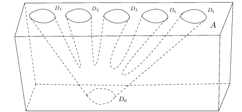
Figure 3: The picture illustrates a 55-pant embedded in MM.

Recall that in Proposition 2.6, we defined a morphism α\alpha from RR to SS where SS is the set of equivalent classes of cobordisms between two countable collections of circles generated by α⁡(xi)=xi~\alpha(x_{i})=\tilde{x_{i}} and α⁡(si)=si~\alpha(s_{i})=\tilde{s_{i}}. In this section, we prove Theorem 2.7, namely, α:R→S\alpha:R\rightarrow S is an isomorphism.

The strategy is to construct a function ϕ\phi from SS to Hom⁡(F∞,F∞)\operatorname{Hom}(F_{\infty},F_{\infty}) such that ϕ∘α=β\phi\circ\alpha=\beta. Since by Theorem 6.13, β\beta is injective, we imply that α\alpha is injective. Together with Proposition 2.6, we conclude that α\alpha is bijective and thus Theorem 2.7 holds.

We first consider the a simpler case when the cobordism does not have braid components.

Definition 7.1.

Let jj be a positive integer and cuboid M=[0,1]3M=[0,1]^{3}. Suppose we have jj input disks Dk​(1≤k≤j)D_{k}(1\leq k\leq j) on the upper surface A={(x,y,1):0≤x,y≤1}A=\{(x,y,1):0\leq x,y\leq 1\} and one output disk D0D_{0} on the lower surface {(x,y,0):0≤x,y≤1}\{(x,y,0):0\leq x,y\leq 1\}. We call the corbodism ρ\rho embedded in MM with input disks Dk​(1≤k≤j)D_{k}(1\leq k\leq j) and output disk D0D_{0} a jj-pant. See Figure 3 for an illustration. The (topological) surface ρ¯=ρ∪⋃0≤k≤jDk\bar{\rho}=\rho\cup\bigcup_{0\leq k\leq j}D_{k} separates MM into two connected components M∖ρ¯=M(1)∪M(2)M\setminus\bar{\rho}=M^{(1)}\cup M^{(2)}. Let M⁡(ρ)M(\rho) denote the connected component which contains some boundary points of MM (i.e. the exterior of surface ρ¯\bar{\rho}). With a little abuse of notations, we also call M⁡(ρ)M(\rho) the exterior of ρ\rho.

Lemma 7.2.

Consider a j-pant ρ\rho embedded in a cuboid MM in the way described in definition 7.1. Let A~=A\∪l=1jDl\tilde{A}=A\backslash\cup_{l=1}^{j}D_{l}. Then the inclusion i:A~↪M⁡(ρ)i:\tilde{A}\hookrightarrow M(\rho) induces an isomorphism i∗:π1​(A~)→π1​(M⁡(ρ))i_{\ast}:\pi_{1}(\tilde{A})\rightarrow\pi_{1}(M(\rho)).

Proof.

We prove by induction on jj.

For j=1j=1, this is true because ρ\rho is a tube in MM and there is an obvious contraction from M⁡(ρ)M(\rho) to A~\tilde{A}.

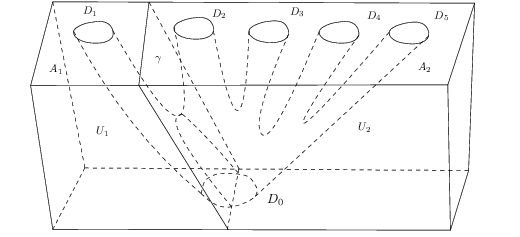
Suppose this holds for j−1j-1. Consider a surface γ\gamma “splitting” M⁡(ρ)M(\rho) into two parts U1U_{1} and U2U_{2} such that U1∩U2=γ∩M⁡(ρ)U_{1}\cap U_{2}=\gamma\cap M(\rho) and U1∪U2=M⁡(ρ)U_{1}\cup U_{2}=M(\rho) in the way shown in Figure 4.

Refer to caption
Figure 4: ρ\rho is a jj-pant and the affine plane γ\gamma separates M⁡(ρ)M(\rho) into U1U_{1} and U2U_{2} where U2U_{2} is essentially the exterior of a (j−1)(j-1)-pant.

Let U1∩A~=A1U_{1}\cap\tilde{A}=A_{1}, U2∩A~=A2U_{2}\cap\tilde{A}=A_{2} and A1∩A2=τA_{1}\cap A_{2}=\tau. Note that U2U_{2} is essentially the exterior of a (j−1)(j-1)-pant embedded in a cuboid. Thus by induction hypothesis, i2:A2↪U2i_{2}:A_{2}\hookrightarrow U_{2} induces an isomorphism i2∗:π1(A2)→π1(U2)i_{2\ast}:\pi_{1}(A_{2})\rightarrow\pi_{1}(U_{2}). Meanwhile, the case when j=1j=1 gives the isomorphism i1∗:π1(A1)→π1(U1)i_{1\ast}:\pi_{1}(A_{1})\rightarrow\pi_{1}(U_{1}) induced by inclusion i1:A1↪U1i_{1}:A_{1}\hookrightarrow U_{1}. Evidently, i0∗:π1(τ)→π1(γ∩M(ρ))i_{0\ast}:\pi_{1}(\tau)\rightarrow\pi_{1}(\gamma\cap M(\rho)) induced by inclusion i0:τ↪γ∩M⁡(ρ)i_{0}:\tau\hookrightarrow\gamma\cap M(\rho) is an isomorphism between trivial groups. Now by using the van Kampen theorem and the naturality of pushout, we deduce that i∗i_{\ast} is an isomorphism. Thus the induction principle proves the lemma. ∎

Recall notations from Section 2. Let A1=N∩Γ1A^{1}=N\cap\Gamma_{1} and A2=N∩Γ2A^{2}=N\cap\Gamma_{2}. We use a2=(0,0,0)a_{2}=(0,0,0) as the base point of A2A^{2} and a1=(0,0,1)a_{1}=(0,0,1) the base point of A1A^{1}. Let BkjB_{k}^{j} be the disk in AjA^{j} with boundary CkjC^{j}_{k} for k=1,2,…k=1,2,\ldots and j=1,2j=1,2. See Figure 6.

Refer to caption
Figure 5: The dashed curves illustrate the generators of fundamental group π1​(Aj~)\pi_{1}(\widetilde{A^{j}}).

Denote Aj~=Aj\⋃k=1∞Bkj\widetilde{A^{j}}=A^{j}\backslash\bigcup_{k=1}^{\infty}B^{j}_{k} for j=1,2j=1,2. For j=1,2j=1,2 and i≥1i\geq 1, we use eije_{i}^{j} to denote the ii-th generator of π1​(Aj~)\pi_{1}(\widetilde{A^{j}}) drawn in Figure 5.

For j=1,2j=1,2, the infinite free group F∞=⟨e1,e2,…⟩F_{\infty}=\langle e_{1},e_{2},\ldots\rangle is isomorphic to π1​(Aj~,aj)\pi_{1}(\widetilde{A^{j}},a_{j}) by mapping

ek→ekj​∀k≥1.e_{k}\rightarrow e_{k}^{j}\;\forall k\geq 1. (38)

This gives us identification

π1​(A1~,a1)≈F∞≈π1​(A2~,a2).\pi_{1}(\widetilde{A^{1}},a_{1})\approx F_{\infty}\approx\pi_{1}(\widetilde{A^{2}},a_{2}). (39)
Refer to caption
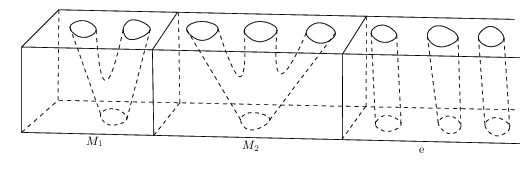
Figure 6: The picture illustrates the shrinking braid s1~​x2~\widetilde{s_{1}}\widetilde{x_{2}}.

Recall that 𝒞\mathcal{C} is the set of all cobordisms. For each r∈𝒞r\in\mathcal{C}, we denote by N⁡(r)N(r) the exterior of r∪⋃{Bkj:k≥1,j=1,2}r\cup\bigcup\{B^{j}_{k}:k\geq 1,j=1,2\} in NN. For t∈[0,1]t\in[0,1], denote Nt​(r)=N⁡(r)∩([0,∞)×[−1,1]×{t}CLOSEN_{t}(r)=N(r)\cap([0,\infty)\times[-1,1]\times\{t\}). For j=1,2j=1,2, denote the embedding map by i​(r)j=Aj~↪N⁡(r)i(r)^{j}=\widetilde{A^{j}}\hookrightarrow N(r) which induces i​(r)∗j:π1​(Aj~,aj)→π1​(N⁡(r),aj)i(r)^{j}_{\ast}:\pi_{1}(\widetilde{A^{j}},a_{j})\rightarrow\pi_{1}(N(r),a_{j}).

Theorem 7.3.

Given r∈𝒞r\in\mathcal{C}, suppose the equivalent class of rr is in SS (i.e. rr is a shrinking braid). Then i​(r)∗1i(r)_{\ast}^{1} is an isomorphism between groups π1​(A1~,a1)\pi_{1}(\widetilde{A^{1}},a_{1}) and π1​(N⁡(r),a1)\pi_{1}(N(r),a_{1}).

Proof.

Recall that, two shrinking braids r1r_{1} and r2r_{2} are said to be equivalent if and only if there is a diffeomorphism G:N→NG:N\rightarrow N such that GG is the identity map on ∂N\partial N and G⁡(r1)=r2G(r_{1})=r_{2}. For any w∈𝒞w\in\mathcal{C}, let w~\widetilde{w} denote the equivalent class of ww. Suppose r~=α⁡(y)\widetilde{r}=\alpha(y) for some y∈Ry\in R. Since yy can be written in the form y=s​xy=sx with s∈B∞s\in B_{\infty} and x∈X∞x\in X_{\infty}, there is a diffeomorphism G:N→NG:N\rightarrow N (which is identity map on ∂N\partial N) such that r′=G⁡(r)r^{\prime}=G(r) is the concatenation of u′,v′u^{\prime},v^{\prime} where u′~=α⁡(s)\widetilde{u^{\prime}}=\alpha(s) and v′~=α⁡(x)\widetilde{v^{\prime}}=\alpha(x). We prove theorem for r′r^{\prime} instead of rr. Since GG is a diffeomorphism preserving boundary of NN, the theorem still holds for rr. Note that N⁡(r′)N(r^{\prime}) is the concatenation of N⁡(u′)¯\overline{N(u^{\prime})} and N⁡(v′)¯\overline{N(v^{\prime})} along the surface C=N1/2​(r′)=N⁡(u′)¯∩N⁡(v′)¯C=N_{1/2}(r^{\prime})=\overline{N(u^{\prime})}\cap\overline{N(v^{\prime})}. Here, N⁡(u′)¯\overline{N(u^{\prime})} and N⁡(v′)¯\overline{N(v^{\prime})} are scaling images of N⁡(u′)N(u^{\prime}) and N⁡(v′)N(v^{\prime}) along zz direction, respectively. See Figure 7. The embedding i(1):C↪N⁡(u′)¯i^{(1)}:C\hookrightarrow\overline{N(u^{\prime})} induces i∗(1):π1​(C)→π1​(N⁡(u′)¯)i_{\ast}^{(1)}:\pi_{1}(C)\rightarrow\pi_{1}(\overline{N(u^{\prime})}) and i(2):C↪N⁡(v′)¯i^{(2)}:C\hookrightarrow\overline{N(v^{\prime})} induces i∗(2):π1​(C)→π1​(N⁡(v′)¯)i_{\ast}^{(2)}:\pi_{1}(C)\rightarrow\pi_{1}(\overline{N(v^{\prime})}).

Refer to caption
Figure 7: r′r^{\prime} is the concatenation of scaling images of u′u^{\prime} and v′v^{\prime}, and N⁡(r′)N(r^{\prime}) is the concatenation of N⁡(u′)¯\overline{N(u^{\prime})} and N⁡(v′)¯\overline{N(v^{\prime})}.

i∗(1)i_{\ast}^{(1)} is an isomorphism by a well-known result on braids. To prove our theorem, it suffices to prove i∗(2)i_{\ast}^{(2)} is an isomorphism. If this is true, then by using van Kampen theorem on N⁡(r′)=N⁡(u′)¯∪N⁡(v′)¯N(r^{\prime})=\overline{N(u^{\prime})}\cup\overline{N(v^{\prime})}, we have

π1​(N⁡(r′))≈π1​(N⁡(u′)¯)∗π1​(C)π1​(N⁡(v′)¯)\displaystyle\pi_{1}(N(r^{\prime}))\approx\pi_{1}(\overline{N(u^{\prime})})\ast_{\pi_{1}(C)}\pi_{1}(\overline{N(v^{\prime})})
≈\displaystyle\approx π1​(N⁡(u′)¯)≈π1​(A1~)\displaystyle\pi_{1}(\overline{N(u^{\prime})})\approx\pi_{1}(\widetilde{A^{1}})

and our theorem follows. Here, the last isomorphism π1​(N⁡(u′)¯)≈π1​(A1~)\pi_{1}(\overline{N(u^{\prime})})\approx\pi_{1}(\widetilde{A^{1}}) is again by results on braids.

Now, as in equation (4), we can write x=x1i1x2i2⋯xkikx=x_{1}^{i_{1}}x_{2}^{i_{2}}\cdots x_{k}^{i_{k}} with integers ij≥0i_{j}\geq 0 for 1≤j≤k1\leq j\leq k.

Let Ml​(l=1,2,…,k)M_{l}(l=1,2,\ldots,k) be kk cuboids. As in definition 7.1, let ρl\rho_{l} be a (il+1)(i_{l}+1)-pant embedded in MlM_{l} with exterior Ml​(ρl)M_{l}(\rho_{l}) for each l=1,2,…,kl=1,2,\ldots,k. Denote by AlA_{l} the upper surface of MlM_{l} and denote Al~=Al∖⋃kDk(l)\widetilde{A_{l}}=A_{l}\setminus\bigcup_{k}D^{(l)}_{k} where {Dk(l):1≤k≤il+1}\{D^{(l)}_{k}:1\leq k\leq i_{l}+1\} are input disks of ρl\rho_{l} in AlA_{l}. Now for l=1,2,…,k−1l=1,2,\ldots,k-1, we glue the right surface of MlM_{l} and the left surface of Ml+1M_{l+1} without changing the relative position of ρl\rho_{l} inside MlM_{l}. Denote the resulting space MM and denote by ρ=∐l=1kρl\rho=\coprod_{l=1}^{k}\rho_{l} the disjoint union of kk cobordisms embedded in MM. Finally let M0M_{0} be the resulting space by gluing the right surface of MM and the left surface of NN in which there is a trivial shrinking braid (i.e. the identity element ee). See Figure 8 for an illustration. Let cobordism ρ0\rho_{0} be the disjoint union of ρ\rho and the trivial shrinking braid (inside M0M_{0}). Denote by M0​(ρ0)M_{0}(\rho_{0}) the exterior of ρ0\rho_{0} in M0M_{0}. Define A0A_{0} to be the upper surface of M0M_{0} and let A0~\widetilde{A_{0}} be the complement of input disks of ρ0\rho_{0} in A0A_{0}. Now, v′v^{\prime} is essentially ρ0\rho_{0}. i.e. There is a diffeomorphism from M0M_{0} to [0,∞)×[−1,1]×[0,12][0,\infty)\times[-1,1]\times[0,\frac{1}{2}] such that it maps ρ0\rho_{0} to v′v^{\prime}, maps M0​(ρ0)M_{0}(\rho_{0}) to N⁡(v′)¯\overline{N(v^{\prime})}, maps A0A_{0} to [0,∞)×[−1,1]×{12}[0,\infty)\times[-1,1]\times\{\frac{1}{2}\} and maps A0~\widetilde{A_{0}} to CC.

Refer to caption
Figure 8: The picture illustrates M0M_{0} for the case when x=x1​x22x=x_{1}x_{2}^{2}.

In order to prove i∗(2)i^{(2)}_{\ast} is an isomorphism, we only need to prove that f∗′:π1​(A0~)→π1​(M0​(ρ0))f^{\prime}_{*}:\pi_{1}(\widetilde{A_{0}})\rightarrow\pi_{1}(M_{0}(\rho_{0})) is an isomorphism where f′:A0~↪M0​(ρ0)f^{\prime}:\widetilde{A_{0}}\hookrightarrow M_{0}(\rho_{0}) is the embedding. By Lemma 7.2, for each l∈{1,2,…,k}l\in\{1,2,\ldots,k\}, il:Al~↪Ml​(ρl)i_{l}:\widetilde{A_{l}}\hookrightarrow M_{l}(\rho_{l}) induces an isomorphism (il)∗:π1​(Al~)↪π1​(Ml​(ρl))(i_{l})_{\ast}:\pi_{1}(\widetilde{A_{l}})\hookrightarrow\pi_{1}(M_{l}(\rho_{l})). Thus by van Kampen theorem and naturality of push out, we imply that f∗′f^{\prime}_{*} is an isomorphism and our theorem follows. ∎

Finally we prove Theorem 2.7:

Proof of Theorem 2.7.

For each r∈Sr\in S and j=1,2j=1,2, recall that i​(r)j=Aj~↪N⁡(r)i(r)^{j}=\widetilde{A^{j}}\hookrightarrow N(r) induces i​(r)∗j:π1​(Aj~,aj)→π1​(N⁡(r),aj)i(r)^{j}_{\ast}:\pi_{1}(\widetilde{A^{j}},a_{j})\rightarrow\pi_{1}(N(r),a_{j}). By (38) and (39), we can regard i​(r)∗j:F∞→π1​(N⁡(r),aj)i(r)^{j}_{\ast}:F_{\infty}\rightarrow\pi_{1}(N(r),a_{j}) for j=1,2j=1,2. By Theorem 7.3, i​(r)∗1i(r)^{1}_{\ast} is an isomorphism. We further identify fundamental groups π1​(N⁡(r),a1)\pi_{1}(N(r),a_{1}) and π1​(N⁡(r),a2)\pi_{1}(N(r),a_{2}) which have different base points. We identify them by connecting a1,a2a_{1},a_{2} with the path γ⁡(t)=(0,0,1−t)\gamma(t)=(0,0,1-t) for t∈[0,1]t\in[0,1] and denote the resulting isomorphism h:π1​(N⁡(r),a1)≈π1​(N⁡(r),a2)h:\pi_{1}(N(r),a_{1})\approx\pi_{1}(N(r),a_{2}). Define ϕ⁡(r)=(i​(r)∗1)−1∘h−1∘(i​(r)∗2)\phi(r)=(i(r)^{1}_{\ast})^{-1}\circ h^{-1}\circ(i(r)^{2}_{\ast}), then ϕ⁡(r):F∞→F∞\phi(r):F_{\infty}\rightarrow F_{\infty}. Thus we have ϕ:S→Hom⁡(F∞,F∞)\phi:S\rightarrow\operatorname{Hom}(F_{\infty},F_{\infty}).

Since r1​r2r_{1}r_{2} is the concatenation for any two shrinking braids r1,r2∈Sr_{1},r_{2}\in S, we have ϕ⁡(r1​r2)=ϕ⁡(r1)∘ϕ⁡(r2)\phi(r_{1}r_{2})=\phi(r_{1})\circ\phi(r_{2}). By Proposition 6.5 and (38), we have ϕ⁡(α⁡(xi))=β⁡(xi)\phi(\alpha(x_{i}))=\beta(x_{i}) and ϕ⁡(α⁡(si))=β⁡(si)\phi(\alpha(s_{i}))=\beta(s_{i}) for each i∈ℕi\in\mathbbm{N}. Since RR is generated by xi,six_{i},s_{i}’s, we have ϕ∘α=β\phi\circ\alpha=\beta. By Theorem 6.13, β\beta is injective and thus α\alpha is injective. Together with Proposition 2.6, α\alpha is bijective and Theorem 2.7 follows. ∎

References

  • [DDRW08] P. Dehornoy, I. Dynnikov, D. Rolfsen, and B. Wiest. Ordering braids. Number 148. American Mathematical Soc., 2008.
  • [Deh94] P. Dehornoy. Braid groups and left distributive operations. Trans. Am. Math., 345(1):115–150, 1994.
  • [Deh98] P. Dehornoy. Transfinite braids and left distributive operations. Math. Z., 228(3):405–433, 1998.
  • [Deh06] P. Dehornoy. The group of parenthesized braids. Adv. Math., 205(2):354–409, 2006.
  • [Deh12] P. Dehornoy. Braids and self-distributivity, volume 192. Birkhäuser, 2012.
  • [Deh18] P. Dehornoy. The braid shelf. J. Knot Theory Ramif., 27(11):1843005, 2018.
  • [FGR+99] R. Fenn, M. T. Greene, D. Rolfsen, C. Rourke, and B. Wiest. Ordering the braid groups. Pacific J. Math, 191(1):49–74, 1999.
  • [Fun01] J. Funk. The hurwitz action and braid group orderings. Theory Appl. Categories, 9(7):121–150, 2001.
  • [Koc04] J. Kock. Frobenius algebras and 2-d topological quantum field theories, volume 59. Cambridge University Press, 2004.
  • [Lav92] R. Laver. The left distributive law and the freeness of an algebra of elementary embeddings. Adv. Math., 91(2):209–231, 1992.
  • [SW00] H. Short and B. Wiest. Orderings of mapping class groups after thurston. Enseign. Math., 46:279–312, 2000, math/9907104.