Kernel-estimated Nonparametric Overlap-Based Syncytial Clustering
Abstract
Commonly-used clustering algorithms usually find ellipsoidal, spherical or other regular-structured clusters, but are more challenged when the underlying groups lack formal structure or definition. Syncytial clustering is the name that we introduce for methods that merge groups obtained from standard clustering algorithms in order to reveal complex group structure in the data. Here, we develop a distribution-free fully-automated syncytial clustering algorithm that can be used with -means and other algorithms. Our approach estimates the cumulative distribution function of the normed residuals from an appropriately fit -groups model and calculates the estimated nonparametric overlap between each pair of clusters. Groups with high pairwise overlap are merged as long as the estimated generalized overlap decreases. Our methodology is always a top performer in identifying groups with regular and irregular structures in several datasets and can be applied to datasets with scatter or incomplete records. The approach is also used to identify the distinct kinds of gamma ray bursts in the Burst and Transient Source Experiment 4Br catalog and the distinct kinds of activation in a functional Magnetic Resonance Imaging study.
Index Terms:
BATSE, DEMP, DEMP+, DBSCAN*, density peaks algorithm, GRB, GSL-NN, -clips, -means, -means, kernel density estimation, KNOB-SynC, MixModCombi, MGHD, MSAL, overlap, PGMM, SDSS, spectral clustering, TiK-meansI Introduction
Cluster analysis [1, 2, 3, 4, 5, 6, 7] is an unsupervised learning method that partitions datasets into distinct groups of homogeneous observations. Finding such structure in the absence of group information can be challenging but is important in many applications, such as taxonomical classification [8], market segmentation [9], software management [10] and so on. As such, a number of methods, ranging from the heuristic [11, 4, 12, 13, 14, 3] to the more formal, model-based [15, 16, 5, 17, 7] approaches have been proposed and implemented.
Most common clustering algorithms, whether model-agnostic methods like -means [14, 18, 19] or model-based approaches such as Gaussian mixture models [20, 5] yield clusters with regular dispersions or structure. For instance, the -means algorithm is geared towards finding homogeneous spherical clusters or spherically-dispersed groups of equal radius. Such algorithms are not designed to find general-shaped or structured groups, therefore, many additional approaches have been suggested to identify irregularly-shaped groups (see, for example, [21, 22, 23, 24, 25, 26, 27]). Kernel -means clustering [21] enhances the -means algorithm by using a kernel function that nonlinearly maps the original (input) space to a higher-dimensional feature space where it may be possible to linearly separate clusters that were not linearly separable in the original space. Spectral clustering [23] uses -means on the first few eigenvectors of a Laplacian of the similarity matrix of the data. Both methods need the number of clusters to be provided: in the case of spectral clustering, [23] suggests estimating this number as the one with the highest gap between successive eigenvalues.
A separate set of approaches modifies the distribution of the mixture components in model-based clustering (MBC) by replacing the commonly-used multivariate Gaussian component with other more general distributions. Some of these approaches simply add dimension reduction in the form of factor models [28, 29] through parsimonious Gaussian mixture models (PGMM). More generally, [30] propose MBC using a mixture of asymmetric shifted Laplace distributions (MixSAL) while [31] suggest using a mixture of generalized hyperbolic distributions (MixGHD). These approaches more fully exploit MBC but can be CPU intensive and are somewhat limited in capturing complex structures.
Evidence accumulation clustering or EAC [22] combines results from multiple runs of the -means algorithm with the underlying rationale that each partitioning provides independent evidence of structure that is then extricated by cross-tabulating the relative frequencies (out of the multiple partitionings) that each observation pair is in the same group. This relative frequency table serves as a similarity matrix for hierarchical clustering: however, implementation of this method can be computationally demanding in terms of CPU speed and memory. [32] developed a nonparametric clustering approach under the premise that each group corresponds to a mode of the estimated multivariate density of the observations. The high-density modes are located and hierarchically clustered with dissimilarity between two modes calculated in terms of the lowest density or number of common points in each mode’s domain of attraction. The “density-based spatial clustering algorithm of applications with noise” (DBSCAN) algorithm [33] groups together points in high-density regions while identifying points in low-density regions as outliers. A refinement (DBSCAN*, by [34]) follows the same principle but classifies so-called border observations as outliers. Both algorithms depend on the minimum cluster size and reachability distance, and also on a cut-off to determine the border and outlying observations. The authors suggest setting this cutoff at the knee of a plot of the -nearest neighbor distances of the observations. In a similar vein, [35] developed a fast Density Peaks (DP) algorithm to determine cluster centers and find outliers while considering the local density of each observation. DP uses the estimated multivariate density in order to classify observations into outliers and does not rely on an explicit cut-off value, but other parameters need to be subjectively specified or estimated to graphically decide on the number of groups. These methods all rely on density estimates and are not immune from the ravages of the curse of dimensionality.
More recent work [24, 25, 26, 27] proposed merging groups found using MBC or -means. Such methods fall into the category of what we introduce in this paper as syncytial clustering algorithms, because they yield a cluster structure resembling a syncytium, a term that in cell biology refers to a multi-nucleated mass of cytoplasm inseparable into individual cells and that can arise from multiple fusions of uninuclear cells. Syncytial clustering algorithms are similar in that they merge or fuse groups that originally corresponded to mixture model components or -means or other regular-structured groups. Resulting partitions have groups with potentially multiple well-defined and structured sub-groups. We outline a few such algorithms next.
MBC is premised on the idea of a one-to-one correspondence between a mixture component of given density form and group. Such injective mapping assumptions are not always tenable so some authors [24, 25, 26] model each group as a mixture of (one or more) components. Operationally, we have a syncytial clustering framework where identified mixture components that are not very distinct from each other are merged [24, 25, 26] into a cluster. [24] successively merge mixture component pairs that result in the highest change in entropy, continuing for as long as the entropy increases. This method, abbreviated here as MMC, is implemented in the R [36] package RMixModCombi [37]. [25] developed the directly estimated misclassification probabilities (DEMP) algorithm to identify candidate components for merging. The author argued that the best measure of group similarity should relate to the classification probability and so proposed that clusters with the highest pairwise misclassification probabilities be merged. The DEMP+ method [26] mimics DEMP but replaces the misclassification probabilities of DEMP with the overlap measure of [38] for Gaussian mixture components. DEMP+ uses Monte Carlo simulation to determine pairwise overlap between merged components and uses thresholds on the maximum pairwise overlap to determine termination. The sliding threshold was empirically suggested to be chosen to be inversely related to dimension.
The MBC algorithms offer a principled approach to the partitioning of observations into groups but are more demanding in CPU time and perhaps unnecessary to use when the objective is simply to find the most appropriate grouping with no particular dogma regarding shape or structure and where using -means as a starting point for an initial clustering may be a fairly plausible but faster alternative. Perhaps recognizing this aspect, [26] contended that DEMP+ can be applied to -means output by assuming equal mixing proportions and homogeneous spherical dispersions in the mixture model. The basis for this assertion is the framing of the -means algorithm of [19] as a Classification Expectation-Maximization (CEM) Algorithm (see [39] for details). But -means clustering makes hard assignments of each observation and, indeed, most commonly-used statistical software programs, such as R [36] use the efficient [18] algorithm that handles computations quite differently and sparingly than [19]. In this vein, [27] provided the K-mH algorithm to merge poorer-separated -means groups. Such groups are identified as per an easily-computed index that uses normal theory with spherical dispersion assumptions. However, the K-mH algorithm has a large number of settings and parameters: using default values and rules-of-thumb provided by the authors, we have found that this method performs well in many datasets but not as well in many others. Therefore, it would be worth investigating other syncytial clustering algorithms that use -means groupings for clustering efficiency while also reducing the need to tune multiple parameter settings.
A separate issue is the impact of Gaussian mixture model assumptions in methods such as DEMP+ when applied to regular-structured groups found using, say, the multivariate -mixture or other appropriate models. A nonparametric method not taking recourse to such distributional assumptions would be desirable in addressing this shortcoming. This paper therefore proposes the Kernel-estimated Nonparametric Overlap-Based Syncytial Clustering (KNOB-SynC) algorithm that successively merges groups from a well-optimized -means solution until some objective and nonparametric data-driven cluster overlap measure vanishes or is no longer reduced. This measure is calibrated through the generalized overlap [40, 41, 42] calculated using smooth estimation of the cumulative distribution function (CDF) developed in Section II. Our algorithm is illustrated and comprehensively evaluated in Section III. Although motivated using -means, the method is general enough to apply to the output of other partitioning algorithms, such as clustering using the [43] distance, or in scenarios with scatter [44] or incomplete records [45]. Section IV also applies our methodology to two interesting settings: in the first case, we identify the differents kinds of gamma ray bursts in the most recent Burst and Transient Source Experiment (BATSE) 4Br catalog. Our second application uses KNOB-SynC to identify activation from single replications of a functional Magnetic Resonance Imaging (fMRI) study obtained from a right-hand finger tapping experiment performed by a right-hand-dominant male. We find our results to both be interpretable and with greater reproducibility than current methods. The paper concludes with some discussion. An appendix provides mathematical proofs for our derived theoretical properties of smooth estimation of the CDF using asymmetric kernel density estimation and detailed graphical illustrations of experimental performance on two-dimensional (2D) datasets and numerical summaries of performance on all datasets.
II Methodological Development
II-A Problem Setup
Let be a random sample of -dimensional observations, with each
| (1) |
where is the number of groups, with if holds and otherwise, is the cluster-specific density of an observation in the th cluster and is the set of observations in the sample from that group. Our specification in (1) refers to a hard clustering framework: we marginally obtain a mixture model if we specify independent identical multinary prior distributions on each . Our objective is to estimate s (equivalently, s) for each with possibly unknown. We also assume that for each , the density for any (i.e. ) can be further described by
| (2) |
where is defined on the positive half of the real line so that is a zero-centered density in with spherical level hyper-surfaces. This means that each group in the dataset can be further decomposed into multiple homogeneous spherically-dispersed subgroups, and if is in and in the th subgroup inside , and zero otherwise. That is, we can model as , or equivalently as
| (3) |
where and for are renumerations, respectively, of all the and for . Therefore, , for and (however, both and are also unknown). The reformulation of (1) in terms of (3) means that the -means algorithm [13, 19, 18] can be employed along with cluster-selection methods (for example, [46, 47, 48]) to obtain a first-pass clustering of the dataset where the observations are partitioned into an estimated number () of homogeneous spherically-dispersed groups. Our proposal is to develop methods for identifying the supersets of these -means (homogeneous spherical) groups to obtain the clusters with also needing to be estimated. These supersets will reveal the general-shaped clustering structure in the data.
From the -groups solution, define the th residual () as
| (4) |
where is the multivariate mean vector of the observations in the th group and . From (4), we obtain the normed residuals, that is, we obtain
| (5) |
for . These may be viewed as a random sample with density function and CDF and having support in . We now provide methods for estimating under assumptions of a smooth CDF.
II-B Smooth estimation of the CDF of the normed residuals
We first introduce a smooth estimator for an univariate CDF. Let be a random sample having CDF and probability density function (PDF) . The natural and most common estimator is the empirical CDF (ECDF) defined as
| (6) |
It is easy to see that is an unbiased estimator of , that is, . Further, it converges almost surely to the true CDF . However, the ECDF is a step function for any and so inappropriate for a smooth continuous CDF, even though it is a smooth function in the limit as [49]. An alternative kernel estimator [50, 51, 49, 52] for replaces the indicator function in (6) by its smooth cousin. Strictly speaking, kernel density estimation is most often employed in nonparametric contexts [49] but can also be extended to smooth CDF estimation by integrating over the domain of the kernel. Let be the CDF of a kernel function . The kernel CDF estimator is then defined as
| (7) |
where is the bandwidth or the smoothing parameter. Equation (7) makes the popular assumption of a symmetric kernel, the most common examples of which are the Gaussian and Epanechnikov [53, 54, 55] kernels. However, using a symmetric kernel when the support of the distribution is not on the entire real line (as is the case with our normed residuals) causes weights to be assigned outside the domain of the observations, resulting in boundary bias [56]. So [57] proposed using an asymmetric kernel in (7) based on the gamma density, with behavior similar to the Gaussian kernel and a comparable rate of convergence in terms of the mean squared error. However, [57]’s estimator is not a valid density for finite sample sizes [58] so we consider the Reciprocal Inverse Gaussian (RIG) kernel density estimator [59]
| (8) |
with . Since is a smooth function the CDF estimate is defined as . Then, integrating with respect to yields the smooth CDF estimator
| (9) |
where is the standard Gaussian CDF. An added benefit of using the RIG kernel over the gamma kernel is that the estimated CDF is in closed form and can be readily evaluated using standard software. We now investigate some theoretical properties of the asymmetric RIG kernel CDF estimator. Before proceeding however, we revisit the definition of the Inverse Gaussian and RIG densities for the sake of completeness and to fix ideas.
Definition 1.
A nonnegative random variable is said to arise from the Inverse Gaussian distribution with parameters if it has the density
| (10) |
Notationally, we write . Also, we have and .
Definition 2.
A nonnegative random variable is said to be from the Reciprocal Inverse Gaussian distribution with parameters if it has the density
| (11) |
Notationally, . Further, is equivalent in law to where and while .
We now develop some properties of the asymmetric kernel RIG to estimate the CDF.
Lemma 3.
Let be independent identically distributed nonnegative-valued random variables with CDF , and PDF that is infinitely differentiable. Also, consider the RIG kernel density defined by where is the standard normal density evaluated at . Consider estimating using as defined in (9). Then, as , and .
Proof.
See Appendix A-A. ∎
Lemma 3 shows that has lower variance than the ECDF and has point-wise Mean Squared Error (MSE) at that is given by .
II-B1 Bandwidth selection
[59] minimized the Mean Integrated Squared Error (MISE) to provide a rule-of-thumb bandwidth selector for the RIG kernel density estimator of the form
| (12) |
However, (12) involves knowledge of the true density and is directly unusable. [59] proposed obtaining by assuming an initial parametric density, say , for and estimating the parameters of the density from the sample. Exact derivations using a lognormal density for were provided [59] but this approach has been found to produce estimates that are biased downwards. We therefore adopt [59]’s approach but use an initial gamma density for and zero otherwise. Under this setup, and . Therefore, we have
| (13) |
with and estimated from the sample using, for example, the method of moments. This is used in (9) to obtain our smoothed RIG-kernel CDF estimator.
The development of this section, when applied to the normed residuals (in place of ), yields a smooth nonparametric kernel-based estimator of their CDF. We use this kernel-estimated CDF in our development of the nonparametric estimation of the overlap measure between groups.
II-C A nonparametric estimator of overlap between groups
Overlap between two groups is an indicator of the extent to which they are indistinguishable from each other. [38] defined the pairwise overlap of two mixture components as the sum of the misclassification probabilities with
| (14) |
For any two mixture components with densities and and mixing proportions and , we have
where and are the parameter sets associated with the th and th mixture components.
[38] calculated (14) for Gaussian mixture densities, but the definition itself is general enough to include other clustering situations including those as general as when we have cluster distributions given by densities of the type in (1). For an equal-proportioned mixture of homogeneous spherical Gaussian densities, [38] showed that between the th and the th cluster where is the standard Gaussian CDF, and are the th and the th cluster means and is the common (homogeneous) standard deviation for each group, estimated unbiasedly as with being the optimized value of the within-sums-of-squares (WSS) of the -groups solution. The sum of and reduces to . The -means formulation of (3) can be viewed more generally [48] and extends beyond the case of Gaussian-distributed groups, so we develop nonparametric methods for estimating the overlap measure.
II-C1 Pairwise overlap between two -means groups
The pairwise overlap (14) between two groups can generally be calculated from as
| (15) |
where represents the normed residual obtained from the th group, and represents the normed pseudo-residual which we define as the norm of the remainder that is obtained by subtracting the th cluster mean from an observation . Let be the RIG kernel-estimated smooth CDF obtained using the bandwidth selected as per (13). Then, can be estimated using (where in the subscript of denotes that the estimated CDF uses the normed residuals). However, the calculation of is not as straightforward. So we estimate using a naïve average estimator
| (16) |
where . The naïve estimator (16) can be considered as an empirical estimator of . Similar estimates of , and therefore , can be obtained. We call this estimated overlap .
II-C2 Pairwise overlap between two composite groups
As described in (2), a composite group is one that can be further decomposed into sub-populations. We now extend the definition of the pairwise overlap for such groups.
Let be defined as in (14) but for composite groups. That is, we use rather than in order to specify that the overlap measure is between composite clusters and . Now . Suppose now that is the th spherical sub-cluster of with mean , , with being the number of spherical sub-clusters in . We assume that if , then implies that is in the subgroup given by . Under this assumption, the density of is defined through its (th) sub-cluster and so
| (17) |
where is a normed residual (obtained, for instance, from the -means solution) for the th spherically-dispersed subgroup in the th cluster. We use the RIG kernel distribution estimator to obtain . From (14), and using the same ideas as in (16) we get the naïve estimator
| (18) |
and similarly for , from where we calculate . Our definitions of s and are consistent in the sense that if and are both -means groups, then . We use this equivalence in the description of our KNOB-SynC algorithm in Section II-D below.
II-C3 Summarizing overlap in a partitioning
Our development so far has provided us with pairwise overlap measures for -means-type (Section II-C1) and composite (Section II-C2) groups. For a -groups (whether of the composite or -means type) partitioning, we get pairwise overlap measures. Summarizing the pairwise overlap measures is important to provide a sense of clustering complexity so [38] originally proposed regulating (maximum of all pairwise overlaps) and (average of all pairwise overlaps) and demonstrated (see Figures 2 and 3 of [38]) the ability to summarize a wide range of cluster geometries. However, because specifying two measures simultaneously is cumbersome, later versions of the CARP [41] and MixSim [42] software packages borrowed ideas from [40] to obtain the generalized overlap where is the largest eigenvalue of the (symmetric) matrix of pairwise overlaps ( for composite groups) and with diagonal entries that are all 1. lies in [0,1] with zero indicating perfect separation between all group densities and 1 indicating indistinguishability between any of them. In this paper, we obtain the estimated generalized overlap using the estimated matrix with off-diagonal entries given by the kernel-estimated pairwise overlaps or , depending on whether we have simple -means-type or composite groups.
II-D The KNOB-SynC Algorithm
Having provided theoretical development for the machinery that we will use, we now describe our multi-phased KNOB-SynC algorithm:
- 1.
The -means phase: This phase finds the optimal partition of the dataset in terms of homogeneous spherically-dispersed groups and has the following steps:
- (a)
For each , obtain -means partitions initialized each of times with distinct seeds randomly chosen from the dataset and run to termination. The best – in terms of the value of the objective function (WSS) at termination – of each set of runs is our putative optimal -means partition for that . We use .
- (b)
When is small relative to (operationally, ), use [46]’s KL criterion to decide on the optimal . Otherwise, for larger , we use the jump statistic [47] on the optimal -means partitions () obtained in Step 1a to determine the optimal (denoted by ). In calculating the jump statistic, we have used , which has become the default in most applications. We refer to [47] for more detailed discussion on this choice of . The corresponding -means solution is the optimal homogeneous spherically-dispersed partition of the dataset. This concludes the -means phase of the algorithm.
- (a)
- 2.
The initial overlap calculation phase: This phase starts with the output of Step 1. That is, we start with a structural definition of the dataset in terms of optimal homogeneous spherically-dispersed groups. Our objective here is to calculate the overlap between each of these groups using nonparametric kernel estimation methods. We proceed as follows:
- (a)
For each observation , compute its normed residual where is defined as in (4). Also, obtain the normed pseudo-residual for , and .
- (b)
- (c)
- (d)
From the overlap matrix , calculate the generalized overlap . Call it .
- (a)
- 3.
The merging phase: The merging phase is triggered only if some of the overlap measures between overlapping clusters are more than the others (operationally, if where is the maximum of the estimated pairwise overlaps) or if is not negligible, that is, if (operationally ). In that case, this phase merges groups, provides pairwise overlap measures between newly-formed composite groups, the updated overlap matrix and the generalized overlap, continuing for as long as the generalized overlap keeps decreasing (by at least ) or is not negligible. Specifically, this phase iteratively proceeds for with the following steps:
- (a)
Merge the groups with the maximum overlap and every pair of groups that have individual pairwise overlaps substantially larger than the generalized overlap . That is, merge every pair of groups , , such that or , for some as described in the comments section below. Call the new merged group and decrease the index labels of the groups with indices greater than . Decrement by 1 for every merged pair.
- (b)
- (c)
The merging phase terminates if , , or . The terminating is the of (1).
- (a)
- 4.
Final clustering solution: The grouping at the end of the merging phase is the final partition of the dataset. This gives us a total of general-shaped groups in the dataset.
Comments:
We provide some additional remarks on KNOB-SynC and relate it to other algorithms for finding general-shaped clusters and settings:
- 1.
The -means phase finds regular-structured (more specifically, homogeneous spherical) groups and, in this regard, is similar to the initial stages of K-mH [27] and EAC [22]. However, EAC repeats -means with fixed several times and is built upon the premise that each -means run does not end up with the same clustering, especially when we do not have underlying homogeneous spherically-dispersed groups. On the other hand, K-mH uses a separability index built on Gaussian assumptions for each cluster and has a large number of user-specified parameters. KNOB-SynC uses nonparametric CDF estimation with a plugin bandwidth selector and a naïve average estimator to calculate the overlap between spherically-dispersed groups and a naïve estimator for the overlap between composite groups. Our methodology has one parameter () that is chosen in a completely data-driven framework. No parameter requires fine-tuning by the practitioner. Also, the number of general-structured groups is decided upon termination that is objectively declared whenever the generalized overlap vanishes or does not go down further.
- 2.
As with MMC, DEMP or DEMP+, the use of cluster distributions in the overlap calculations simplifies and keeps practical computations even for large datasets. In contrast, EAC, DBSCAN, DBSCAN∗, DP and K-mH require memory-intensive cross-tabulation of the entire dataset across multiple clusterings because frequency tables need to be calculated and/or stored.
- 3.
KNOB-SynC uses a naïve estimator to update the overlap between composite groups, unlike DEMP+ which uses Monte Carlo simulations and is slower. Further, DEMP+ uses the maximum overlap that is very sensitive to individual pairwise overlap measures while KNOB-SynC uses the generalized overlap measure [40] that provides a nonlinear summary of all the individual pairwise overlaps.
- 4.
Unlike DEMP or DEMP+, the stopping criterion of KNOB-SynC is data-driven, thus allowing for the possibility of obtaining well-separated and less well-separated partitionings as supported by the data. Our algorithm also has the potential, unlike MMC, DEMP or DEMP+, to merge multiple pairs of groups in a step.
- 5.
KNOB-SynC uses nonparametric CDF estimation but does so in univariate space by exploiting the inherent spherically-dispersed structure (ellipsoidal in the case of clustering with the Mahalanobis distance) of the sub-clusters. Therefore, it has greater immunity against the curse of dimensionality that bedevils multivariate density estimation that is used in algorithms such as DBSCAN∗ and DP.
- 6.
The parameter determines the types of composite groups that are formed. For larger values of , we have groups formed by merging a few pairs at each iteration while smaller values prefer many simultaneous mergers. (For , no merging is possible.) In the first case, we expect to have stringy groups while in the second case, we find clusters that are irregular-shaped but less stringy. A data-driven approach to choosing , that we adopt, runs the algorithm with different values of and uses the final partitioning with the smallest terminating as the optimal clustering.
- 7.
Unlike other syncytial clustering algorithms like DEMP, DEMP+ or K-mH, KNOB-SynC allows for the possibility of multiple pairs of groups to be merged at an iteration.
- 8.
Our initial stage uses -means for speed and efficiency that also allows us to explore larger candidate values of . However, the approach could very well have been used with clustering algorithms obtained using, say, the generalized Mahalanobis distance. The overlap calculations are then easily modified. To see this, suppose that the generalized Mahalanobis distance between two points and is given by , where is any appropriate nonnegative-definite matrix with (say, Moore-Penrose) inverse given by . (A positive definite leads to the usual Mahalanobis distance.) Under the generalized Mahalanobis distance framework, (14) reduces to
(19) which means that the problem reduces to the Euclidean case if we use what we here refer to as the normed Mahalanobis-free residuals (and pseudo-residuals). Operationally, this is equivalent to obtaining , and replacing the with in the calculation of (5) and proceeding as before. This framework also includes the case when we scale each variable before clustering, as happens when the features are on vastly different scales, or when we use principal components (PCs) as our clustering variables – we illustrate these scenarios in Sections III-C6 and IV-A.
- 9.
Our algorithm accommodates clustering scenarios in the presence of scatter as provided, for instance, by the output of the -clips algorithm of [44]. Scatter observations are those that are unlike any other and may be considered as individual groups in their own right. KNOB-SynC incorporates these scatter observations as individual clusters in addition to the groups found from the output of the -clips algorithm and proceeds with the overlap calculation and merging phases as described earlier in this section. We illustrate this scenario in Section III-D1.
- 10.
Datasets often have incomplete records with missing observations in some features. The -means algorithm [45] provides a -means type algorithm for Euclidean distance clustering in this setting. Then, instead of -means, KNOB-SynC can incorporate results from -means in the first stage. For the incompletely-observed records, we calculate the rescaled normed residual in the presence of missing information by removing the missing value from their calculation and re-weighting it appropriately. Specifically, we calculate the th rescaled normed residual as
(20) where represent the available features for the th record that has been assigned to the th spherically-dispersed sub-group with estimated mean . Similar arguments allow for the calculation of the rescaled normed pseudo-residual . The use of the nonparametric CDF estimator in KNOB-SynC provides us with the flexibility to calculate the initial overlap estimates from these scaled-up normed residuals. The merging phase and termination criteria of our algorithm remain unchanged. Section III-D2 illustrates KNOB-SynC on a dataset with incomplete records.
- 11.
The use of nonparametric methods in the overlap calculations means that a large number of methods may be possible to use in the initial partitional phase. The method can also potentially be modified to apply to other kinds of datasets. For instance, the initial clustering can be done for categorical datasets using -modes [60, 61, 62, 63] and then the Generalized or Gaussianized Distributional Transform [64, 65] and copula model [66] can potentially be applied to each cluster to obtain numerical-valued residuals for use with our overlap estimation and calculations.
Having proposed our KNOB-SynC algorithm, we now illustrate and evaluate its performance in relation to a host of competing methods.
III Performance Evaluations
We first illustrate the performance of KNOB-SynC on the 2D Aggregation dataset of [67] and then follow with more detailed performance evaluations on a large number of datasets usually used to evaluate competing algorithms in the literature. These datasets range from two to many dimensions. We compare our methods with a wide range of suitors. These rival methods are the syncytial clustering techniques of K-mH [27] using author-supplied R code, MMC [24] as implemented in the R package MixModCombi, DEMP [25] using the R package fpc and DEMP+ [26]. We also evaluate performance with EAC [22] and GSL-NN [32] using publicly available author-supplied code. We also apply two common connectivity-based techniques of spectral and kernel -means clustering. Both these methods need the number of groups to proceed: for spectral clustering we decide this number to be the one with the highest gap in successive eigenvalues of the similarity matrix [23]. For kernel -means, we set to be the true value: we recognize that our evaluation of kernel -means potentially provides this method with an unfair advantage, however, we proceed in this fashion in order to understand the best case scenario of this competing method. Finally, we also compare our method’s performance relative to DBSCAN∗ as implemented in the R package dbscan [68], DP clustering [35] as implemented in the R package densityClust [69], PGMM [29] using the R package pgmm [70], MSAL using the R package MixSAL [71] and MGHD using the R package MixGHD [72]. Many of these algorithms have multiple parameters that need to be set – in our experiments, we use the default settings where guidance for choosing these parameters is not explicitly available. Also, the DBSCAN∗ and DP clustering algorithms identify scatter/outliers that by definition are those observations that are unlike any other in the dataset, so we follow [44] in considering them as individual singleton clusters in our performance assessments. Performance for each method is evaluated by [73]’s adjusted Rand index measured between the true partition and the estimated final partitioning. In general, : values closer to 1 indicating greater similarity between partitionings and good clustering performance. The index takes values farther from 1 as performance becomes poorer and is expected to take a value of zero for a random assignmment. The index can take arbitrarily negative values, but as very helpfully pointed out to us by a reviewer, the probability of observing is relatively small (see [74] for further discussion on the characteristics of this index).
III-A Illustrative Example: the Aggregation dataset
displays the results of the different phases and iterations of KNOB-SynC. We display the stages of KNOB-SynC for which is when we have the lowest terminating (from among ) for this example. The -means phase of our algorithm identifies 14 clusters with partitioning as in Figure 1a and estimates the initial overlap matrix to be as in Figure 1d. The first merging phase yields the partitioning in Figure 1b with the updated of Figure 1e. The next merging phase only combines one pair of groups and is terminal, resulting in the final partitioning of the dataset as in Figure 1c. The overlap matrix (Figure 1f) indicates well-separated clusters, with only six mislabeled observations relative to the true, and a of 0.98 between the true and estimated classifications.
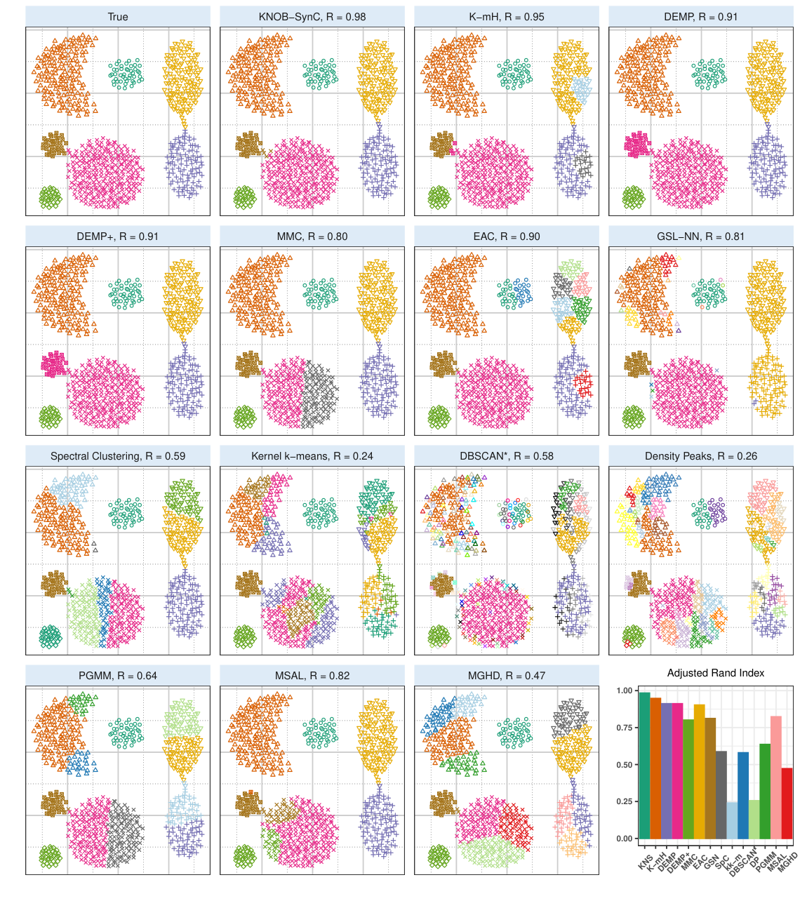
The competing methods (Figure 2) all perform marginally to substantially worse. K-mH is the second best performer () finding groups but breaking the top right cluster into two and also grouping a few other stray observations. Both DEMP and DEMP+ yield the same result (), but MMC (, ) has trouble with the largest group, splitting it into two sub-groups. EAC breaks the top central and large groups on the right into many clusters, resulting in but . Thus, in spite of identifying a large number of groups, EAC is able to capture a fair bit of the complex group structure of this dataset. GSL-NN can not distinguish between the groups on the right but also finds many other small groups elsewhere, ending with groups and . The performance of spectral clustering is worse: it finds groups and has a with the true classification. Despite being provided with the true , kernel -means with is the worst performer in this example, with DP (, ) only marginally better. DBSCAN* at and , correctly finds the large circular group and one of the smallest groups, but the observations in the top left group are almost all classified as outliers/scatter. Among the MBC methods for general-shaped clusters, MSAL at is the best performer, finding groups but having trouble with the larger group at the bottom. PGMM finds groups () with the larger groups split further, while the worst-performing MBC method is MGHD (, .
III-B Additional 2D Experiments
III-B1 Experimental framework
Figure 3 displays the 12 additional 2D datasets used to
evaluate performance of KNOB-SynC and its competitors. Barring the first example, all these datasets have been used by other authors to demonstrate and evaluate performance of their methods. The groups in these datasets have structure ranging from the regular (for example, the 7-spherically-dispersed Gaussian clusters dataset that is modeled on a similar example in [75] and where sophisticated methods like KNOB-SynC are superfluous and unnecessary) to widely-varying complexity. The Banana Arcs dataset has observations clumped in four banana-shaped structures arced around each other. The Banana-clump and Bullseye datasets are from [32] – the former has 200 observations with one spherical group and another arced around it on the left like a banana, while the latter has 400 observations grouped, as its name implies, as a bullseye. The more complex-structured Bullseye-Cigarette dataset [27] has three concentric-ringed groups, two elongated groups above two spherical groups on the left, and another group that is actually a superset of two overlapping spherical groups ( and ). The Compound dataset [76] is very complex-structured with observations in groups that are not just varied in shape, but a group that sits atop another on the right. The Half-ringed clusters dataset [77] has 373 observations in two arc-shaped clusters, one of which is dense and the other being very sparsely-populated. The Path-based dataset [78] has 300 observations in three groups, two of which are regular-shaped and surrounded by a widely arcing third group. The Spiral dataset [78] has 312 observations in three spiral groups that are very difficult for standard clustering algorithms to recover accurately. The SSS dataset has 5015 observations in three S-shaped groups of varying density and orientations while the XXXX dataset has observations distributed in four cross-shaped structures.
III-B2 Results
Figure 4 and Table VIII summarize the performance of all methods on the 2D experimental datasets. Detailed displays of different methods on individual datasets are in Appendix B. The summaries indicate across-the-board good performance of KNOB-SynC with it always being a top performer. In its worst case, KNOB-SynC gets a (on the Path-based dataset) where it terminates early (Figure 18) but here also it is the fourth-best performer,
behind spectral clustering (), MGHD () and PGMM (). The competing syncytial clustering methods do well in some cases, but not in others where other methods perform better. Among the syncytial clustering methods, K-mH performs better than DEMP, DEMP+ and MMC whose performance can sometimes be poor (e.g., on the Bullseye, Half-ringed clusters and Spiral datasets – vide Figures 14, 17 and 20). It is on these datasets that the other methods (EAC, GSL-NN, and spectral clustering) do better. The performance of kernel--means even with known true number of groups is varied, being very good sometimes (e.g., in the Bananas-clump dataset of Figure 13) but very poor in other cases (e.g., as seen before in the Aggregation dataset) where almost every other method does well. The three general MBC methods perform similarly but PGMM does a bit better than MSAL and MGHD. DBSCAN∗ and, especially DP, generally perform poorly – however, DBSCAN∗ performs well in some cases. We quantify performance of each method against its competitors in terms of its average deviation from the best performer. Specifically, for each dataset, we compute the deviation (or difference) in of a method from that of the best performer for that dataset. The average deviation () of a method over all datasets is an overall indicator of its performance. Table VIII provides and the standard deviation or SD () of the differences. On the average, KNOB-SynC is the best performer (and with the lowest ) followed by GSL-NN, K-mH and EAC. This conclusion of KNOB-SynC’s superior overall performance is also supported by Figure 4. We surmise that KNOB-SynC does well across the different datasets because of its ability by construction to merge many or few components at a time, with the exact choice of merges and termination objectively selected and determined by the distinctiveness of the resulting partitioning as per .
III-C Higher-Dimensional Datasets
We also study the performance of KNOB-SynC and its competitors on higher-dimensional datasets. These datasets are modest- to higher-dimensional, with between 173 to 10993 records. For the higher-dimensional datasets (i.e., with non-redundant dimension greater than 10), we find that all methods other than GSL-NN generally perform better when used on the first few () kernel principal components (KPCs) rather than on the raw data. For these methods and these datasets, we use the first KPCs of each dataset with chosen as the first time after which increases in the eigenvalues corresponding to the successive KPCs are below 0.5%. GSL-NN is implemented on the original datasets. Further, KNOB-SynC, K-mH and EAC are built on -means whose results depend on the scale of the features. So, for these methods, we scaled each feature by the SD prior to analysis unless the features were all collected on a similar scale, as with the E. coli example of Section III-C2 or the log-transformed GRB dataset of Section IV-A. (Following the usual rule-of-thumb in multivariate statistics, we assume that features are on similar scales if the most variable feature has SD no more than four times that of the feature with lowest variability.) Each dataset and the performance of each method is first described individually. A comprehensive summary of the performance of each method on each dataset follows in Section III-C11.
III-C1 Simplex-7 Gaussian Clusters
This dataset, from [32], is of Gaussian realizations of size 50, 60, 70, 80, 90, 100 and 110 each from seven clusters with means set at the vertices of the seven-dimensional unit simplex and homogeneous spherical dispersions with common SD of 0.25 in each dimension. Like the 7-Spherical dataset, this dataset exemplifies a case where standard methods such as -means or Gaussian MBC should be adequate. Therefore it is a test of whether our algorithm and its competitors are able to refrain from identifying spurious complexity. All methods, except for EAC, DBSCAN* and DP, identify seven groups and have good clustering performance. In particular, the syncytial methods have very good performance (); other methods have . EAC still performs well () but finds groups. DBSCAN* is the worst performer () on this dataset, finding many outliers (). DP’s performance is middling at and with many outliers ().
III-C2 E. coli Protein Localization
The E. coli dataset, publicly available from the University of California Irvine’s Machine Learning Repository (UCIMLR) [79], concerns identification of protein localization sites for the E. coli bacteria [80]. There are eight protein localization sites: cytoplasm, inner membrane without signal sequence, periplasm, inner membrane with an uncleavable signal sequence, outer membrane, outer membrane lipoprotein, inner membrane lipoprotein, and inner membrane with a cleavable signal sequence. Identifying these sites is an important early step for finding remedies [80]. Each protein sequence has a number of numerical attributes – see [81] for a listing and their detailed description. Two attributes are binary, but 326 of the 336 sequences have common values for these attributes. We restrict our investigation to these sequences and drop the two binary attributes from our list of variables. These 326 sequences have no representation from the inner membrane or outer membrane lipoproteins. Additionally, we also drop two sequences because they are the lone representatives from the inner membrane with cleavable sequence site [82].
| 1 | 2 | 3 | 4 | 5 | 6 | 7 | 8 | 9 | |
|---|---|---|---|---|---|---|---|---|---|
| cytoplasm | 138 | 0 | 0 | 4 | 0 | 0 | 0 | 0 | 1 |
| inner membrane, no signal sequence | 7 | 62 | 0 | 0 | 0 | 3 | 3 | 1 | 0 |
| inner membrane, uncleavable signal sequence | 1 | 32 | 0 | 0 | 0 | 0 | 0 | 1 | 0 |
| outer membrane | 0 | 0 | 17 | 2 | 0 | 0 | 0 | 0 | 0 |
| periplasm | 3 | 1 | 2 | 38 | 8 | 0 | 0 | 0 | 0 |
Therefore we have observations from true classes. KNOB-SynC identifies groups. Table I presents the confusion matrix containing the number of times a protein from a localization site is assigned to each KNOB-SynC group. Ignoring stray assignments, the sites are fairly well-defined in the first four groups, with . Uncleavable signal sequences from the inner membrane site are difficult to distinguish from those that are also from there but have no signal sequence. Sequences from the other sites are better-clarified. Among the alternative methods, EAC does slightly better ( but identifies 10 groups. The remaining methods all do slightly to substantially worse. DEMP, DEMP+ and K-mH each identify four groups but with . K-mH finds only two groups () while the rest find more groups but disagree more strongly with the true localizations. DBSCAN∗ finds a large number of groups () with relatively poor performance (). DP is marginally better () while PGMM () and MGHD () improves on DP, each finding 8 groups. (MSAL did not converge to a solution.) Overall, EAC and KNOB-SynC are the top two performers, with DEMP and DEMP+ close behind.
III-C3 Standard Wine Recognition
The standard wine recognition dataset [83, 84], also available from the UCIMLR contains measurements on wine samples that are obtained from its chemical analysis. There are 59, 71 and 48 wines of the Barolo, Grignolino and Barbera cultivars, so . Because here, we use KPCs. KNOB-SynC is the best performer, finding groups with a clustering performance of . The first group contains all the 59 wines from the Barola cultivar and 2 Grignolino wines. The second group contains 66 wines, all exclusively from the Grignolino cultivar. The third group has 2 Grignolino and 48 Barbera wines. Thus, there is very good definition among the KNOB-SynC groups. On the other hand, only MMC (), K-mH (), PGMM ( and EAC () perform modestly while the others are substantially worse with DBSCAN∗, in particular, classifying all observations as outliers, resulting in and .
III-C4 Extended Wine Recognition
A reviewer very helpfully pointed out that the dataset used in Section III-C3 is actually a reduced variant, and a fuller version of the dataset with 27 variables is available in the R package pgmm. We used KPCs in our experimental evaluations on this larger dataset. DEMP and DEMP+ () show perfect classification while MGHD () and MMC () also perform well. KNOB-SynC is a top performer and the best among the distribution-free methods, finding groups and with a clustering performance of . The first group here has 58 Barola and 2 Grignolino wines. The second group contains 68 wines from the Grignolino cultivar and the one Barolo wine that was not placed in the first group. The third group has the 48 Barbera wines and the one remaining Grignolino wine. Similar to the 13-dimensional case, we get good definition among the groups. Other methods not discussed here do moderately to substantially worse.
III-C5 Olive Oils
The olive oils dataset [85, 86] has measurements on 8 chemical components for 572 samples of olive oil taken from 9 different areas in Italy that are from three regions: Sardinia and Northern and Southern Italy. This is an interesting dataset with sub-classes (areas) inside classes (regions). Indeed, [27] were able to identify, with one misclassification, sub-groups within the regions but not the areas (; we however get using the authors’ supplied code) – they surmised that it may be more possible to identify characteristics of olive oils based on regions defined by physical geography rather than areas demarcated by political geography. We therefore analyze performance on this dataset both in terms of how regions and areas are recovered. KNOB-SynC identifies regions (Table II) with oils from the Sardinian and Northern regions correctly classified into the first two groups. The Southern region oils are split into our two remaining groups, one containing all but 2 of the 25 North Apulian samples and 6 of the 36 Sicilian samples, and the other group containing all the Southern oils.
| Region | Area | 1 | 2 | 3 | 4 |
|---|---|---|---|---|---|
| Sardinia | Coast-Sardinia | 33 | 0 | 0 | 0 |
| Inland-Sardinia | 65 | 0 | 0 | 0 | |
| North | East-Liguria | 0 | 0 | 50 | 0 |
| West-Liguria | 0 | 0 | 50 | 0 | |
| Umbria | 0 | 0 | 51 | 0 | |
| South | Calabria | 0 | 56 | 0 | 0 |
| North-Apulia | 0 | 2 | 0 | 23 | |
| South-Apulia | 0 | 206 | 0 | 0 | |
| Sicily | 0 | 30 | 0 | 6 |
In terms of clustering performance, KNOB-SynC gets when compared to the true areal grouping but when compared to the true regional grouping. For this dataset DEMP (), DEMP+ () and MSAL () are the top performers with respect to the true areal grouping. The remaining methods all have middling performance. When compared with the true regional grouping, KNOB-SynC is by far the best performer. Overall, the clustering performance of KNOB-SynC for the regional grouping marginally trumps the performance of DEMP for the areal grouping and so may be considered to be more accurate in uncovering the group structure in the dataset.
III-C6 Image Segmentation
The image segmentation dataset, also available from the UCIMLR, is on 19 attributes of the scene in each image manually classified to be from BRICKFACE, CEMENT, FOLIAGE, GRASS, PATH, SKY and WINDOW. (Thus, .) We combine the training and test datasets to obtain 330 instances of each scene, so . There is a lot of redundancy in the attributes so we reduce the dataset to 8 PCs that together explain at least 99.9% of the total variance in the dataset. The PCs are obtained from the correlation matrix because the 19 attributes have vastly different scales. The KNOB-SynC solution finds clusters, with . The confusion matrix (Table III) indicates that the SKY images are perfectly identified while GRASS and, to a lesser extent, PATH and CEMENT, are fairly well-identified. On the other hand, the partitioning struggles to distinguish between BRICKFACE, FOLIAGE and WINDOW.
| 1 | 2 | 3 | 4 | 5 | 6 | 7 | 8 | 9 | 10 | 11 | 12 | |
|---|---|---|---|---|---|---|---|---|---|---|---|---|
| BRICKFACE | 330 | 0 | 0 | 0 | 0 | 0 | 0 | 0 | 0 | 0 | 0 | 0 |
| CEMENT | 42 | 257 | 0 | 4 | 0 | 27 | 0 | 0 | 0 | 0 | 0 | 0 |
| FOLIAGE | 300 | 5 | 0 | 0 | 0 | 5 | 2 | 7 | 3 | 1 | 3 | 4 |
| GRASS | 1 | 0 | 327 | 0 | 0 | 2 | 0 | 0 | 0 | 0 | 0 | 0 |
| PATH | 0 | 0 | 0 | 269 | 0 | 61 | 0 | 0 | 0 | 0 | 0 | 0 |
| SKY | 0 | 0 | 0 | 0 | 330 | 0 | 0 | 0 | 0 | 0 | 0 | 0 |
| WINDOW | 309 | 13 | 0 | 0 | 0 | 8 | 0 | 0 | 0 | 0 | 0 | 0 |
Among other methods, only EAC () and MGHD () are modestly to marginally better than KNOB-SynC. Inspection of the EAC grouping indicates many small groups but also difficulty in separating FOLIAGE and WINDOW, placing them together in one group. Further, BRICKFACE is split into five groups, four of which are predominantly of this kind, but the fifth group is unable to distinguish 146 observations of BRICKFACE from 32, 52 and 62 observations of CEMENT, FOLIAGE and WINDOW, respectively. The other methods all perform moderately to substantially worse (Table IX) with PGMM, MSAL and DBSCAN∗ unable to find clustering solutions.
III-C7 Yeast Protein Localization
The yeast protein localization dataset [87], also obtained from the UCIMLR, was used by [26] to illustrate the application of DEMP+. This dataset is on the localization of the proteins in yeast into one of sites and has two attributes (presence of “HDEL” substring and peroxisomal targeting signal in the C-term) that are essentially binary and trinary. Following [26], we drop these variables and use the other variables, namely signal sequence recognition scores based on (a) McGeoch’s and (b) von Heijne’s methods, (c) ALOM membrane spanning region prediction score, and discriminant analysis scores of the amino acid content of (d) N-terminal region (20 residues long) of mitochondrial and non-mitochondrial proteins and (e) vacuolar and extracellular proteins and (f) discriminant scores of nuclear localization signals of nuclear and non-nuclear proteins. For this dataset, all methods perform poorly. KNOB-SynC () is the best performer – the other clustering methods essentially randomly allocate observations. Surprisingly, DEMP+ (, ) performs very poorly. ([26] only used the first five of our variables to illustrate the DEMP+ method: we find no appreciable improvement even then, with and . Personal queries to the author did not successfully resolve this discrepancy.) It appears therefore that the yeast protein localization dataset may be difficult to accurately partition in a completely unsupervised framework.
III-C8 Acute Lymphoblastic Leukemia
The Acute Lymphoblastic Leukemia (ALL) training dataset of [88] was used by [32] to illustrate GSL-NN in a high-dimensional small sample size framework. We use the standardized dataset in [32] that measured the oligonucleotide expression levels of the 1000 highest-varying genes in 215 patients suffering from one of seven leukemia subtypes, namely, T-ALL, E2A-PBX1, BCR-ABL, TEL-AML1, MLL rearrangement, Hyperploid chromosomes, or an unknown category labeled OTHER. Some subtypes have very few cases: for instance, only 9, 14 and 18 patients are of type BCR-ABL, MLL and E2A-PBX1, respectively. For this dataset, we use KPCs for all methods but GSL-NN. The -means stage of KNOB-SynC identifies six groups, none of which are merged in the merging phase, resulting in the best partitioning among all competing methods. Table IV
| 1 | 2 | 3 | 4 | 5 | 6 | |
|---|---|---|---|---|---|---|
| Hyperdiploid 50 | 0 | 0 | 2 | 35 | 5 | 0 |
| E2A-PBX1 | 0 | 17 | 0 | 0 | 1 | 0 |
| BCR-ABL | 0 | 0 | 2 | 1 | 6 | 0 |
| TEL-AML1 | 4 | 2 | 8 | 2 | 36 | 0 |
| MLL | 0 | 3 | 10 | 0 | 1 | 0 |
| T-ALL | 0 | 0 | 1 | 0 | 0 | 27 |
| OTHER | 51 | 0 | 0 | 0 | 1 | 0 |
presents the confusion matrix containing the number of cases a patient of a leukemia subtype was assigned to a KNOB-SynC group. We see that most leukemia subtypes are distinctively identified in the KNOB-SynC solution. The alternative methods perform mildly to substantially worse with PGMM, spectral clustering, GSL-NN and DP having clustering solutions () that are the next best after KNOB-SynC. Other methods generally do poorly, with MSAL and MGHD unable to find solutions while DBSCAN∗ classifies all observations as outliers.
III-C9 Zipcode images
The zipcode images [32] dataset consists of images of handwritten Hindu-Arabic numerals and is our second higher-dimensional example. As in the ALL dataset of Section III-C8, we normalize the observations to have zero mean and unit variance so that the Euclidean distance between any two normalized images is negatively and linearly related to the correlation between their pixels. We extract and use the first KPCs for all algorithms but GSL-NN. KNOB-SynC identifies 9 groups and has the best clustering performance (). DP is the second best () performer but finds groups (including singletons) followed by MGHD (), K-mH (), GSL-NN and spectral clustering (both with but and 23). The other methods all perform moderately to substantially worse.

Figure 5 displays the 9 KNOB-SynC groups. While misclassifications abound in almost all groups, there is good agreement with 0, 1, 2, the leaner 8s and, (to a lesser extent) 3 and 6, largely correctly identified. The digit 2 is placed in two groups, of the leaner and the rounded versions. The group where 3 predominates also has some 5s and 8s but the categorization makes visual sense. Another group is composed largely of 4s, 7s and 9s but that placement also appears visually explainable. Clearer and straighter 7s and 9s are placed in a separate group. Our partitioning finds it harder to distinguish between 5 and 6 but here also the commonality of the strokes in the digits assigned to this group explains this categorization. Thus we see that KNOB-SynC is not only the best performer for this dataset but also provides interpretable results. We comment that our application of all methods to this dataset has been entirely unsupervised: methodologies that also account for spatial context and pixel neighborhood may further improve the grouping but are outside the purview of this paper.
III-C10 Handwritten Pen-digits
| 0 | 1 | 2 | 3 | 4 | 5 | 6 | 7 | 8 | 9 | 11 | 12 | 13 | 14 | 15 | |
|---|---|---|---|---|---|---|---|---|---|---|---|---|---|---|---|
| 0 | 1099 | 1 | 0 | 0 | 19 | 0 | 21 | 0 | 0 | 2 | 0 | 1 | 0 | 0 | 0 |
| 1 | 0 | 657 | 358 | 34 | 1 | 0 | 2 | 2 | 0 | 89 | 0 | 0 | 0 | 0 | 0 |
| 2 | 0 | 2 | 1141 | 0 | 0 | 0 | 0 | 0 | 0 | 1 | 0 | 0 | 0 | 0 | 0 |
| 3 | 0 | 4 | 2 | 1046 | 1 | 0 | 0 | 0 | 0 | 2 | 0 | 0 | 0 | 0 | 0 |
| 4 | 0 | 5 | 1 | 2 | 1118 | 0 | 1 | 0 | 0 | 17 | 0 | 0 | 0 | 0 | 0 |
| 5 | 0 | 1 | 0 | 252 | 0 | 625 | 0 | 0 | 2 | 175 | 0 | 0 | 0 | 0 | 0 |
| 6 | 0 | 0 | 1 | 0 | 0 | 1 | 1054 | 0 | 0 | 0 | 0 | 0 | 0 | 0 | 0 |
| 7 | 0 | 144 | 5 | 2 | 0 | 0 | 0 | 914 | 0 | 0 | 0 | 0 | 77 | 0 | 0 |
| 8 | 4 | 0 | 0 | 3 | 0 | 1 | 0 | 1 | 461 | 0 | 139 | 321 | 48 | 24 | 53 |
| 9 | 24 | 9 | 0 | 72 | 3 | 0 | 0 | 0 | 1 | 714 | 0 | 0 | 0 | 232 | 0 |
UCIMLR is a larger dataset that has 16 attributes from 250 handwritten samples of 30 writers. (There are records because eight samples are unavailable.) We use KPCs in our analysis [27, used the first 7 PCs and got and ]. KNOB-SynC finds groups and is the best performer (). It separates the digits 0, 2, 3, 4, 6 and, to a lesser extent, 7 fairly well but identifying 1, 5 and 9 is a bit more challenging (Table V). It also identifies multiple types of 8. MGHD finds the correct number and is the next-best performer . The other methods perform moderately to substantially worse with MSAL unable to find a clustering solution.
III-C11 Summary of Performance
Figure 6 and Table IX summarize performance of all methods on the higher-dimensional experiments. As in the 2D case, KNOB-SynC is almost always among the top performers for high-dimensional datasets. Indeed, KNOB-SynC has the lowest average difference in from that of the best-performing method over all datasets (Table IX). The other methods generally perform worse, with EAC, PGMM and kernel--means (with true number of groups) among the better ones. Thus, the results of our experiments on real and synthetic datasets indicate good performance of KNOB-SynC relative to its competitors.
III-D Extensions of KNOB-SynC
As indicated in Section II, the development of our syncytial clustering methodology is based on the nonparametric estimation of the CDF of the residuals and so can be applied to other scenarios. We explore performance of our methodology in two such settings.
III-D1 KNOB-SynC in the presence of scatter
[44] provided the -clips algorithm for -means clustering in the presence of scatter, or observations that are unlike any other in the dataset. Our KNOB-SynC methodology and software readily incorporates -clips results by replacing the -means phase with that algorithm, and proceeding by including the scatter points as individual singleton clusters. We illustrate our methodology on the first 100 images of the Olivetti faces database [91] that were used by [35] to illustrate their DP algorithm. The 100 images under our consideration are of 10 faces each of 10 individuals taken at different angles and under different light conditions. Therefore, each individual can be considered to be a group with members that are that person’s 10 images. Each image has a total of 10,304 pixels so we use the first 37 KPCs. While this application does not have any true scatter points, we use this application to illustrate KNOB-SynC with -clips because it was used by [35] to showcase DP that finds scatter (outliers, in their parlance) in addition to clusters.
The -clips algorithm with the default Bayesian Information Criterion (BIC) [92] finds only two well-defined homogeneous spherical clusters and 68 scatter points. We use the trace of the within-sums-of-squares-and-products matrix, rather than its determinant [44], in our objective function in order to satisfy the condition of homogenous spherical clusters around which our base KNOB-SynC algorithm is built. Thus, we have a total of 70 initial groups. KNOB-SynC’s merging phase ends with 9 large groups, 5 small groups and 1 scatter observation (so ) and .
| Assigned Groups | ||||||||||||||||
| Individual | 1 | 2 | 3 | 4 | 5 | 6 | 7 | 8 | 9 | 10 | 11 | 12 | 13 | 14 | 15 | 16 |
| 1 | 9 | 0 | 0 | 0 | 0 | 0 | 0 | 0 | 0 | 0 | 0 | 0 | 1 | 0 | 0 | 0 |
| 2 | 0 | 10 | 0 | 0 | 0 | 0 | 0 | 0 | 0 | 0 | 0 | 0 | 0 | 0 | 0 | 0 |
| 3 | 0 | 0 | 8 | 0 | 0 | 0 | 0 | 0 | 0 | 0 | 2 | 0 | 0 | 0 | 0 | 0 |
| 4 | 0 | 0 | 0 | 10 | 0 | 0 | 0 | 0 | 0 | 0 | 0 | 0 | 0 | 0 | 0 | 0 |
| 5 | 0 | 0 | 0 | 0 | 3 | 0 | 0 | 0 | 0 | 0 | 0 | 2 | 0 | 2 | 1 | 2 |
| 6 | 0 | 0 | 0 | 0 | 0 | 10 | 0 | 0 | 0 | 0 | 0 | 0 | 0 | 0 | 0 | 0 |
| 7 | 0 | 0 | 0 | 0 | 0 | 0 | 10 | 0 | 0 | 0 | 0 | 0 | 0 | 0 | 0 | 0 |
| 8 | 0 | 0 | 0 | 0 | 0 | 0 | 0 | 10 | 0 | 0 | 0 | 0 | 0 | 0 | 0 | 0 |
| 9 | 0 | 0 | 0 | 0 | 0 | 0 | 0 | 0 | 10 | 0 | 0 | 0 | 0 | 0 | 0 | 0 |
| 10 | 0 | 0 | 0 | 0 | 0 | 0 | 0 | 0 | 0 | 9 | 0 | 0 | 0 | 0 | 1 | 0 |
The results are displayed in Table VI and Figure 7 – for comparison, the latter also displays the results reported in [35] which found 9 clusters and 62 scatter points, resulting in and . (The figure displays images assigned to a group by means of a distinctive sequential palette. Because there are not enough colors to also identify each scatter point with its individual sequential palette, we use an individual randomized nominal palette for each scatter assignment.)


KNOB-SynC identifies images from six individuals (Persons 2, 4, 6, 7, 8 and 9) perfectly and the first, third and the tenth individuals nearly so. The fifth individual is characterized into 5 smaller groups that includes the case where one image is grouped together with the one misclassified image of the tenth person. The performance of our algorithm overwhelms that reported in [35]. We note that we used the first 37 KPCs with our KNOB-SynC algorithm while [35] used the original images with similarity metric as in [93]. Using DP () or DBSCAN∗ () with Euclidean similarity on the 37 KPCs gave us worse results.
III-D2 KNOB-SynC with incomplete records
We now illustrate a scenario where KNOB-SynC is applied to a dataset with incomplete records. In this example, we replace the -means phase with [45]’s -means algorithm that modifies -means to account for incomplete records. The authors also develop a modified jump statistic to select the number of groups. The -means results are input into the merging phase of KNOB-SynC and the algorithm proceeds as usual.
We illustrate our methodology on a subset [94] of the Sloan Digital Sky Survey (SDSS) dataset that measures five features (brightness, in psfCounts, size in petroRads, texture, and two measures of shape ( and that we refer to as Shape1 and Shape2 in our analysis) on 1220 galaxies and 287 stars. Thus the true and . The dataset has some missing values for the shape measures of 42 galaxies.
The -means algorithm with the modified jump statistic of [45] finds homogeneous spherically-dispersed groups. The initial overlap calculations of Step 2 of our algorithm yield and . The merging phase is triggered, and terminates with groups.


| KNOB-SynC Groups | ||||
|---|---|---|---|---|
| 1 | 2 | 3 | 4 | |
| Galaxies | 1159 | 2 | 56 | 3 |
| Stars | 0 | 287 | 0 | 0 |
Figure 8 provides a 3D radial visualization [65] of the clustering results and a confusion matrix of the obtained grouping vis-a-vis the true classification. We see that KNOB-SynC groups all the 287 stars together, but also includes 2 galaxies. The remaining galaxies are all partitioned into groups of 1159, 56 and 3 observations. The large galaxy group and the group with stars are all well-separated from the ones in the smaller galaxy groups. The second-largest KNOB-SynC galaxy group has larger-sized galaxies while the three galaxies in the last group have larger Shape1 and brightness. This illustration demonstrates KNOB-SynC’s ability to identify general-shaped clusters even in the presence of incomplete records. We note that some of the competing methods such as K-mH or EAC may be modified to incorporate -means results but such modifications to both the methodology and software is outside the scope of this paper.
Our experimental evaluations comprehensively demonstrate that our KNOB-SynC algorithm works very well in finding general-shaped clusters. Indeed, our methodology can also incorporate scenarios that allow for scatter or incomplete records in the dataset.
IV Real-world applications
In this section we apply KNOB-SynC to first find the different kinds of Gamma Ray Bursts (GRBs) in an astronomy catalog and second, to identify activation detected in fMRI experiments. The ground truth is unknown in both these applications, so we compare our results with other available evidence in the literature.
IV-A Determining the distinct kinds of Gamma Ray Bursts
There is tremendous interest in understanding the source and nature of Gamma Ray Bursts (GRBs) that are the brightest electromagnetic events known to occur in space [95, 96]. Many researchers [97, 98, 99] have hypothesized that GRBs are of several kinds, but the exact number and descriptive properties of these groups is an area of active research and investigation. Most analyses have traditionally focused on univariate and bivariate statistical and descriptive methods for classification and found two groups but other authors [100, 95] have found three different kinds of GRBs when using more variables in the clustering. Recent careful analyses [101, 102] has conclusively established five ellipsoidally-shaped groups in the GRB dataset obtained from the BATSE 4Br catalog. Indeed, [102] established that all nine fields of the BATSE 4Br catalog have important clustering information using methods developed in [103]. These nine fields are the two duration variables (time by which 50% and 90% of the flux arrive), the four time-integrated fluences in the 20-50, 50-100, 100-300, and keV spectral channels, and the (three) measurements on peak fluxes in time bins of 64, 256 and 1024 milliseconds. The authors used multivariate -mixtures MBC on the logarithm of the measurements, and BIC for model selection, to arrive at their result of five ellipsoidally-shaped groups.
GRB datasets have typically been analyzed after using a transformation to remove skewness in the dataset. This summary transformation is somewhat arbitrary so [104] used their Transformation-infused -means (TiK-means) algorithm to alternately transform features and cluster skewed datasets. A modification [104] of the jump statistic that accounts for the use of transformations in the algorithm found five groups that were characterized as long-intermediate-intermediate, short-faint-intermediate, short-faint-soft, long-bright-hard and long-intermediate-hard in terms of their duration (), total fluence () and spectral hardness () which are the summaries used to characterize GRB groups [100].
The fields of the BATSE 4Br catalog are heavily correlated in the log-scale. This has led many researchers to argue for and summarily ignore all but a few variables in their analysis. Here we explore performance using KNOB-SynC on the first three PCs (accounting for 96.27% of the total variance) of the nine scaled log-transformed variables which is equivalent to using KNOB-SynC with the generalized Mahalanobis distance. The -means phase applied on the 3 PCs finds 5 groups. KNOB-SynC does not enter the merging stage at all since the maximum and generalized overlaps are the same. Comparison of our results (Figure 9 and Table VII) with those of [104] shows fairly good agreement in the confusion matrix (). The first and the fourth groups have short burst durations () and soft spectral hardness () although the first group has fainter total fluence (). Groups 2 and 3 have long durations and bright fluences but different spectral hardness. Group 5 has long duration GRBs but with intermediate fluence and spectral hardness. The true number and kinds of GRB groups is not known but our results show that the KNOB-SynC solution yields groups that are distinct, interpretable and in line with the newer results obtained by TiK-means [104] or MBC [101, 102].
| KNOB-SynC | 1 | 207 | short-intermediate-soft | |||
| 2 | 187 | long-bright-soft | ||||
| 3 | 459 | long-intermediate-hard | ||||
| 4 | 318 | short-faint-soft | ||||
| 5 | 428 | long-bright-hard | ||||
| TiK-means | 1 | 197 | short-intermediate-soft | |||
| 2 | 188 | long-bright-soft | ||||
| 3 | 429 | long-intermediate-hard | ||||
| 4 | 333 | short-faint-soft | ||||
| 5 | 452 | long-bright-hard |
| KNOB-SynC | ||||||
|---|---|---|---|---|---|---|
| 1 | 2 | 3 | 4 | 5 | ||
| Tik-means | 1 | 188 | 2 | 2 | 3 | 2 |
| 2 | 0 | 181 | 0 | 0 | 7 | |
| 3 | 1 | 0 | 420 | 2 | 6 | |
| 4 | 13 | 0 | 7 | 313 | 0 | |
| 5 | 5 | 4 | 30 | 0 | 413 | |
IV-B Activation detection in a fMRI finger-tapping task experiment
Our second application uses KNOB-SynC to identify activation in fMRI experiments. One objective of fMRI is to determine cerebral regions that respond to a task or particular stimulus [105, 106, 107, 108]. A typical approach relates, after correction and pre-processing, the observed Blood Oxygen Level Dependent (BOLD) time course sequence at each image voxel to the expected BOLD response [109, 110, 111] by fitting a general linear model [112] and obtaining a test statistic (often a -statistic) that tests for significance at that voxel. Thresholding methods [113, 114] are often used on these -statistics to determine activation. Attempts to use clustering algorithms have been made, but [115] found that despite the advantages of speed and simplicity, -means is not, in general, a good performer because it fits “data idiosyncracies” and pathologies. We therefore explore if KNOB-SynC can improve the -means clustering solution on these datasets.
Our dataset for this experiment is from a right-hand finger-tapping experiment of a right-hand-dominant male and was acquired over twelve regularly-spaced sessions in a two-month span. We choose only 5 of these sessions that were identified in [40] as the ones with the highest reliability. Because there is no known gold standard, our comparison here will be of the five partitionings detected in each replication with each other. Each dataset was preprocessed and voxel-wise -scores were obtained that quantified the test statistic under the hypothesis of no activation at each voxel. We refer to [116] and [117] for imaging details. At each of the voxels, we compute the -scores to test the hypothesis that the expected BOLD levels are significantly related to the right-hand tapping at a voxel. These -scores for each replication are our (one-dimensional) dataset. Because of the large size of the dataset, most competing methods are impractical to apply, so we only use KNOB-SynC here. (For computational reasons also, we do not estimate in the -means phase but set it at .)


The 50 homogeneous -means groups in each of the five replicates when supplied to the merging phase each terminated with syncytial groups. For the first replicate, the largest group has 178307 (99.4%) voxels – this is essentially the region of no activation. The other replicates have 178898 (99.7%), 178129 (99.3%), 179087 (99.8%), and 178658 (99.6%) voxels in this group. Figure 10a displays the -scores at the activated voxels over four slices of the brain. The displayed slices comprise the ipsi- and contra-lateral pre-motor cortices (pre-M1), the primary motor cortex (M1), the pre-supplementary motor cortex (pre-SMA), and the supplementary motor cortex (SMA). We see broad agreement between the replications in each of the four slices. We compare our KNOB-SynC results with the robust adaptive smoothed thresholding (AR-FAST) algorithm of [118] implemented by the R package RFASTfMRI [119] which shows far less agreement among the 5 replicates in terms of detected activation in the four slices. Specifically, KNOB-SynC (Figure 10a) identifies activation in the left M1 and in the ipsi-lateral pre-M1 areas. There is some identified activation in the contra-lateral pre-M1, pre-SMA and SMA voxels. On the other hand, AR-FAST (Figure 10b) finds less activation in the left M1 and in the ipsi-lateral pre-M1 areas. Figure 10c displays the [120] index of the activation detected (using KNOB-SynC) between each pair of replications. Figure 10d displays similar Jaccard index calculations with regard to activation detected using AR-FAST. The Jaccard indices are higher for KNOB-SynC-found activation for each pair of replications and show greater reproducibility. The summarized Jaccard index of [40] which provides an overall measure of reproducibility of activation detected across replicates is 0.238 for KNOB-SynC and 0.102 for AR-FAST which was shown [118] to be a top performer on this dataset. We comment that while the overall Jaccard indices are low for both methods, the low value of 0.238 also reflects the challenge of activation detection in single-subject fMRI. Seen in this context, KNOB-SynC does quite well. This example illustrates the potential of KNOB-SynC to improve and refine clustering solutions making it possible, for instance, to use -means and to alleviate some of the concerns raised in [115].
V Discussion
This paper has proposed a syncytial clustering algorithm called KNOB-SynC that merges groups found by standard clustering algorithms such as -means, and does so in a data-driven and fully objective way. A R package called SynClustR implements our method in the function KNOBSynC and the competing K-mH syncytial algorithm in the function kmH and is publicly available at https://github.com/ialmodovar/SynClustR. Our method is distribution-free and can apply to the results of many standard clustering algorithms. We use the overlap measure of [38] for merging and for decisions but use kernel-based nonparametric methods to calculate this overlap. Our algorithm has no parameters that require fine-tuning by the user and, as pointed out by a reviewer, shows robust performance across many datasets of many dimensions and with little to tremendous complexity, when compared against a host of other methods. Further, our methodology is general enough to extend to situations with incomplete records or where clustering is done in the presence of scatter. Application of KNOB-SynC to data from the BATSE 4Br catalog provides further evidence of five kinds of GRBs. Our approach is also demonstrated to potentially make it possible to adapt -means clustering for activation detection in fMRI.
This paper also developed estimation methods of the CDF using the asymmetric RIG kernel. We used the plugin-bandwidth selector that minimizes the MISE as our bandwidth choice but it would be good to develop and investigate more sophisticated approaches. Further, our development in this paper provides an opportunity to develop nonparametric methods for diagnostics in clustering. For instance, our developed kernel CDF estimator could be used to determine uncertainties in -means classifications. A reviewer has also very kindly drawn our attention to the fact that the construction of composite clusters that underlies the idea behind syncytial clustering has also been used in the context of semi-supervised clustering [121] where, instead of estimated overlap as used in this paper, available class labels are used in deciding to merge pairs of groups. We believe that such an approach may also benefit from our methodology, especially when not all classes have representation in the supervised portion of the dataset. Thus, we see that although we have made an important contribution, a number of issues remain that would benefit from further attention.
References
- [1] D. B. Ramey, “Nonparametric clustering techniques,” in Encyclopedia of Statistical Science. New York: Wiley, 1985, vol. 6, pp. 318–319.
- [2] G. J. McLachlan and K. E. Basford, Mixture Models: Inference and Applications to Clustering. New York: Marcel Dekker, 1988.
- [3] L. Kaufman and P. J. Rousseuw, Finding Groups in Data. New York: John Wiley & Sons, 1990.
- [4] B. S. Everitt, S. Landau, and M. Leesem, Cluster Analysis (4th ed.). New York: Hodder Arnold, 2001.
- [5] V. Melnykov and R. Maitra, “Finite mixture models and model-based clustering,” Statistics Surveys, vol. 4, pp. 80–116, 2010.
- [6] R. Xu and D. C. Wunsch, Clustering. NJ, Hoboken: John Wiley & Sons, 2009.
- [7] C. Bouveyron, G. Celeux, B. T. Murphy, and A. E. Raftery, Model-Based Clustering and Classification for Data Science: With Applications in R. Cambridge Series in Statistical and Probabilistic Mathematics, 2019.
- [8] C. D. Michener and R. R. Sokal, “A quantitative approach to a problem in classification,” Evolution, vol. 11, pp. 130–162, 1957.
- [9] A. Hinneburg and D. Keim, “Cluster discovery methods for large databases: from the past to the future,” in Proceedings of the ACM SIGMOD International Conference on the Management of Data, 1999.
- [10] R. Maitra, “Clustering massive datasets with applications to software metrics and tomography,” Technometrics, vol. 43, no. 3, pp. 336–346, 2001.
- [11] S. Johnson, “Hierarchical clustering schemes,” Psychometrika, vol. 32:3, pp. 241–254, 1967.
- [12] A. Jain and R. Dubes, Algorithms for clustering data. Englewood Cliffs, NJ: Prentice Hall, 1988.
- [13] E. Forgy, “Cluster analysis of multivariate data: efficiency vs. interpretability of classifications,” Biometrics, vol. 21, pp. 768–780, 1965.
- [14] J. MacQueen, “Some methods for classification and analysis of multivariate observations,” Proceedings of the Fifth Berkeley Symposium, vol. 1, pp. 281–297, 1967.
- [15] D. Titterington, A. Smith, and U. Makov, Statistical Analysis of Finite Mixture Distributions. Chichester, U.K.: John Wiley & Sons, 1985.
- [16] G. McLachlan and D. Peel, Finite Mixture Models. New York: John Wiley and Sons, Inc., 2000.
- [17] P. D. McNicholas, Mixture model-based classification. Chapman and Hall/CRC, 2016.
- [18] J. A. Hartigan and M. A. Wong, “A -means clustering algorithm,” Applied Statistics, vol. 28, pp. 100–108, 1979.
- [19] S. Lloyd, “Least squares quantization in PCM,” Information Theory, IEEE Transactions on, vol. 28, no. 2, pp. 129–137, 1982.
- [20] C. Fraley and A. E. Raftery, “Model-based clustering, discriminant analysis, and density estimation,” Journal of the American Statistical Association, vol. 97, pp. 611–631, 2002.
- [21] I. Dhillon, Y. Guan, and B. Kulis, “A unified view of kernel k-means, spectral clustering and graph cuts,” University of Texas at Austin, Tech. Rep. TR-04-25, 2004.
- [22] A. L. Fred and A. K. Jain, “Combining multiple clusterings using evidence accumulation,” IEEE transactions on pattern analysis and machine intelligence, vol. 27, no. 6, pp. 835–850, 2005.
- [23] U. von Luxburg, “A tutorial on spectral clustering,” Statistics and Computing, vol. 17, no. 4, pp. 395–416, December 2007.
- [24] J.-P. Baudry, A. E. Raftery, G. Celeux, K. Lo, and R. Gottardo, “Combining mixture components for clustering,” Journal of Computational and Graphical Statistics, vol. 19, no. 2, pp. 332 – 353, 2010.
- [25] C. Hennig, “Methods for merging Gaussian mixture components,” Advances in Data Analysis and Classification, 2010.
- [26] V. Melnykov, “Merging mixture components for clustering through pairwise overlap,” Journal of Computational and Graphical Statistics, vol. 25, no. 1, pp. 66–90, 2016.
- [27] A. D. Peterson, A. P. Ghosh, and R. Maitra, “Merging -means with hierarchical clustering for identifying general-shaped groups,” Stat, vol. 7, no. 1, p. e172, 2018.
- [28] Z. Ghahramani and G. E. Hinton, “The EM algorithm for factor analyzers,” University of Toronto, Toronto, Canada, Tech. Rep. CRG-TR-96-1, 1997.
- [29] P. D. McNicholas and T. B. Murphy, “Parsimonious Gaussian mixture models,” Statistics and Computing, vol. 18, no. 3, pp. 285–296, 2008.
- [30] B. C. Franczak, R. P. Browne, and P. D. McNicholas, “Mixtures of shifted asymmetric Laplace distributions,” IEEE Transactions on Pattern Analysis and Machine Intelligence, vol. 36, no. 6, pp. 1149–1157, 2014.
- [31] R. P. Browne and P. D. McNicholas, “A mixture of generalized hyperbolic distributions,” Canadian Journal of Statistics, vol. 43, no. 2, pp. 176–198, 2015.
- [32] W. Stuetzle and R. Nugent, “A generalized single linkage method for estimating the cluster tree of a density,” Journal of Computational and Graphical Statistics, 2010.
- [33] M. Ester, H.-P. Kriegel, J. Sander, X. Xu et al., “A density-based algorithm for discovering clusters in large spatial databases with noise.” in KDD-96, vol. 96, no. 34, 1996, pp. 226–231.
- [34] R. J. Campello, D. Moulavi, and J. Sander, “Density-based clustering based on hierarchical density estimates,” in Pacific-Asia conference on knowledge discovery and data mining. Springer, 2013, pp. 160–172.
- [35] A. Rodriguez and A. Laio, “Clustering by fast search and find of density peaks,” Science, vol. 344, no. 6191, pp. 1492–1496, 2014.
- [36] R Development Core Team, R: A Language and Environment for Statistical Computing, R Foundation for Statistical Computing, Vienna, Austria, 2018, ISBN 3-900051-07-0. [Online]. Available: http://www.R-project.org
- [37] J.-P. Baudry and G. Celeux, RmixmodCombi: Combining Mixture Components for Clustering, 2014, r package version 1.0. [Online]. Available: https://CRAN.R-project.org/package=RmixmodCombi
- [38] R. Maitra and V. Melnykov, “Simulating data to study performance of finite mixture modeling and clustering algorithms,” Journal of Computational and Graphical Statistics, vol. 19, no. 2, pp. 354–376, 2010.
- [39] C. Fraley and A. E. Raftery, “How many clusters? which cluster method? answers via model-based cluster analysis,” Computer Journal, vol. 41, pp. 578–588, 1998.
- [40] R. Maitra, “A re-defined and generalized percent-overlap-of-activation measure for studies of fMRI reproducibility and its use in identifying outlier activation maps,” Neuroimage, vol. 50, no. 1, pp. 124–135, 2010.
- [41] V. Melnykov and R. Maitra, “CARP: Software for fishing out good clustering algorithms,” Journal of Machine Learning Research, vol. 12, pp. 69 – 73, 2011.
- [42] V. Melnykov, W.-C. Chen, and R. Maitra, “MixSim: An R package for simulating data to study performance of clustering algorithms,” Journal of Statistical Software, vol. 51, no. 12, pp. 1–25, 2012. [Online]. Available: http://www.jstatsoft.org/v51/i12/
- [43] P. C. Mahalanobis, “On the generalised distance in statistics,” Proceedings of the National Institute of Sciences of India, vol. 2, no. 1, p. 49–55, 1936.
- [44] R. Maitra and I. P. Ramler, “Clustering in the presence of scatter,” Biometrics, vol. 65, pp. 341 – 352, 2009.
- [45] A. Lithio and R. Maitra, “An efficient k-means-type algorithm for clustering datasets with incomplete records,” Statistical Analysis and Data Mining: The ASA Data Science Journal, vol. 11, no. 6, pp. 296–311, 2018.
- [46] W. J. Krzanowski and Y. Lai, “A criterion for determining the number of groups in a data set using sum-of-squares clustering,” Biometrics, pp. 23–34, 1988.
- [47] C. A. Sugar and G. M. James, “Finding the number of clusters in a dataset,” Journal of the American Statistical Association, vol. 98, no. 463, 2003.
- [48] R. Maitra, V. Melnykov, and S. Lahiri, “Bootstrapping for significance of compact clusters in multi-dimensional datasets,” Journal of the American Statistical Association, vol. 107, no. 497, pp. 378–392, 2012.
- [49] B. W. Silverman, Density Estimation for Statistics and Data Analysis. London: Chapman & Hall/CRC, 1986.
- [50] M. Rosenblatt, “Remarks on some nonparametric estimates of a density function,” The Annals of Mathematical Statistics, vol. 27, no. 3, p. 832, 1956.
- [51] E. Parzen, “On estimation of a probability density function and mode,” The Annals of Mathematical Statistics, vol. 33, no. 3, p. 1065, 1962.
- [52] M. P. Wand and M. C. Jones, Kernel Smoothing. London: Chapman & Hall/CRC, 1995.
- [53] V. A. Epanechnikov, “Non-parametric estimation of a multivariate probability density,” Theory of Probability and its Applications, vol. 14, p. 153–158, 1969.
- [54] A. Azzalini, “A note on the estimation of a distribution function and quantiles by a kernel method,” Biometrika, vol. 68, no. 1, pp. 326–328, 1981.
- [55] R.-D. Reiss, “Nonparametric estimation of smooth distribution functions,” Scandinavian Journal of Statistics, pp. 116–119, 1981.
- [56] T. Bouezmarni and O. Scaillet, “Consistency of asymmetric kernel density estimators and smoothed histograms with application to income data,” Econometric Theory, vol. 21, no. 02, pp. 390–412, 2005.
- [57] S. X. Chen, “Probability density function estimation using gamma kernels,” Annals of the Institute of Statistical Mathematics, vol. 52, no. 3, pp. 471–480, 2000.
- [58] Y. Jeon and J. H. T. Kim, “A gamma kernel density estimation for insurance loss data,” Insurance: Mathematics and Economics, vol. 53, pp. 569–579, 2013.
- [59] O. Scaillet, “Density estimation using inverse and reciprocal inverse Gaussian kernels,” Nonparametric Statistics, vol. 16, no. 1-2, pp. 217–226, 2004.
- [60] Z. Huang, “Clustering large data sets with mixed numeric and categorical values,” in Proceedings of the First Pacific Asia Knowledge Discovery and Data Mining Conference. Singapore: World Scientific, 1997, p. 21–34.
- [61] ——, “Extensions to the -means algorithm for clustering large data sets with categorical values,” Data Mining and Knowledge Discovery, vol. 2, p. 283–304, 1998.
- [62] A. Chaturvedi, P. E. Green, and J. D. Caroll, “-modes clustering,” Journal of Classification, vol. 18, pp. 35–55, 2001.
- [63] K. S. Dorman and R. Maitra, “An efficient -modes algorithm for clustering categorical datasets,” ArXiv e-prints:2006.03936, 2020.
- [64] L. Rüschendorf, Mathematical Risk Analysis. Berlin Heidelberg: Springer-Verlag, 2013.
- [65] Y. Zhu, F. Dai, and R. Maitra, “Three-dimensional radial visualization of high-dimensional continuous or discrete datasets,” ArXiv e-prints:1905.09505, Mar. 2019.
- [66] R. B. Nelsen, An Introduction to Copulas, 2nd ed. New York: Springer, 2006.
- [67] A. Gionis, H. Mannila, and P. Tsaparas, “Clustering aggregation,” ACM Transactions on Knowledge Discovery from Data (TKDD), vol. 1, no. 1, p. 4, 2007.
- [68] M. Hahsler and M. Piekenbrock, dbscan: Density Based Clustering of Applications with Noise (DBSCAN) and Related Algorithms, 2018, r package version 1.1-3. [Online]. Available: https://CRAN.R-project.org/package=dbscan
- [69] T. L. Pedersen, S. Hughes, and X. Qiu, densityClust: Clustering by Fast Search and Find of Density Peaks, 2017, r package version 0.3. [Online]. Available: https://CRAN.R-project.org/package=densityClust
- [70] P. D. McNicholas, A. ElSherbiny, A. F. McDaid, and T. B. Murphy, pgmm: Parsimonious Gaussian Mixture Models, 2018, r package version 1.2.3. [Online]. Available: https://CRAN.R-project.org/package=pgmm
- [71] B. C. Franczak, R. P. Browne, P. D. McNicholas, and K. L. Burak, MixSAL: Mixtures of Multivariate Shifted Asymmetric Laplace (SAL) Distributions, 2018, r package version 1.0. [Online]. Available: https://CRAN.R-project.org/package=MixSAL
- [72] C. Tortora, A. ElSherbiny, R. P. Browne, B. C. Franczak, , P. D. McNicholas, and D. D. Amos., MixGHD: Model Based Clustering, Classification and Discriminant Analysis Using the Mixture of Generalized Hyperbolic Distributions, 2019, r package version 2.3.2. [Online]. Available: https://CRAN.R-project.org/package=MixGHD
- [73] L. Hubert and P. Arabie, “Comparing partitions,” Journal of Classification, vol. 2, pp. 193–218, 1985.
- [74] D. Steinley, “Properties of the Hubert-Arabie adjusted Rand index.” Psychological methods, vol. 9, no. 3, p. 386, 2004.
- [75] R. Maitra, “Initializing partition-optimization algorithms,” IEEE/ACM Transactions on Computational Biology and Bioinformatics, vol. 6, pp. 144–157, 2009.
- [76] C. T. Zahn, “Graph-theoretical methods for detecting and describing gestalt clusters,” IEEE Transactions on computers, vol. 100, no. 1, pp. 68–86, 1971.
- [77] A. K. Jain and M. H. C. Law, “Data clustering: A user’s dilemma,” in Pattern Recognition and Machine Intelligence. PReMI 2005, ser. Lecture Notes in Computer Science, S. K. Pal, B. S., and B. S., Eds., vol. 3776. Berlin, Heidelberg: Springer, 2005, pp. 1–10.
- [78] H. Chang and D.-Y. Yeung, “Robust path-based spectral clustering,” Pattern Recognition, vol. 41, no. 1, pp. 191 – 203, 2008. [Online]. Available: http://www.sciencedirect.com/science/article/pii/S0031320307002038
- [79] D. J. Newman, S. Hettich, C. L. Blake, and C. J. Merz, “UCI repository of machine learning databases,” 1998.
- [80] K. Nakai and M. Kinehasa, “Expert sytem for predicting protein localization sites in gram-negative bacteria,” PROTEINS: Structure, Function, and Genetics, vol. 11, pp. 95–110, 1991.
- [81] P. Horton and K. Nakai, “A probablistic classification system for predicting the cellular localization sites of proteins,” Intelligent Systems in Molecular Biology, pp. 109–115, 1985.
- [82] R. Maitra, “A statistical perspective to data mining,” Journal of the Indian Society of Probability and Statistics, vol. 6, pp. 28–77, 2002.
- [83] M. Forina, R. Leardi, and S. Lanteri, “PARVUS - an extendible package for data exploration, classification and correlation,” Via Brigata Salerno, 16147 Genoa, Italy, 1988.
- [84] D. C. S. Aeberhard and O. de Vel, “Comparison of classifiers in high dimensional settings,” Department of Computer Science and Department of Mathematics and Statistics, James Cook University of North Queensland, Tech. Rep. 92-02, 1992.
- [85] M. Forina and E. Tiscornia, “Pattern recognition methods in the prediction of italian olive oil origin by their fatty acid content,” Annali di Chimica, vol. 72, pp. 143–155, 1982.
- [86] M. Forina, C. Armanino, S. Lanteri, and E. Tiscornia, “Classification of olive oils from their fatty acid composition,” in Food Research and Data Analysis. London: Applied Science Publishers, 1983, pp. 189–214.
- [87] K. Nakai, “UCI machine learning repository,” 1996. [Online]. Available: http://archive.ics.uci.edu/ml
- [88] E.-J. Yeoh, M. E. Ross, S. A. Shurtleff, W. Williams, D. Patel, R. Mahfouz, F. G. Behm, S. C. Raimondi, M. V. Relling, A. Patel, C. Cheng, D. Campana, D. Wilkins, X. Zhou, J. Li, H. Liu, C.-H. Pui, W. E. Evans, C. Naeve, L. Wong, and J. R. Downing, “Classification, subtype discovery, and prediction of outcome in pediatric acute lymphoblastic leukemia by gene expression profiling,” Cancer Cell, vol. 1, no. 2, pp. 133 – 143, 2002.
- [89] F. Alimoglu, “Combining multiple classifiers for pen-based handwritten digit recognition,” Master’s thesis, Institute of Graduate Studies in Science and Engineering, Bogazici University, 1996.
- [90] F. Alimoglu and E. Alpaydin, “Methods of combining multiple classifiers based on different representations for pen-based handwriting recognition,” in Proceedings of the Fifth Turkish Artificial Intelligence and Artificial Neural Networks Symposium (TAINN 96), Istanbul, Turkey, 1996.
- [91] F. S. Samaria and A. C. Harter, “Parameterization of a stochastic model for human face identification,” in Proceedings of the Second IEEE Workshop on Applications of Computer Vision, Sarasota, Florida, 1994, pp. 138–142.
- [92] G. Schwarz, “Estimating the dimensions of a model,” Annals of Statistics, vol. 6, pp. 461–464, 1978.
- [93] M. P. Sampat, Z. Wang, S. Gupta, A. C. Bovik, and M. K. Markey, “Complex wavelet structural similarity: A new image similarity index,” IEEE Transactions on Image Processing, vol. 18, no. 11, pp. 2385–2401, 2009.
- [94] K. Wagstaff, “Clustering with missing values: No imputation required,” in Classification, clustering, and data mining applications. Springer, 2004, pp. 649–658.
- [95] T. Chattopadhyay, R. Misra, A. K. Chattopadhyay, and M. Naskar, “Statistical evidence for three classes of gamma-ray bursts,” Astrophysical Journal, vol. 667, no. 2, p. 1017, 2007.
- [96] T. Piran, “The physics of gamma-ray bursts,” Rev. Mod. Phys., vol. 76, pp. 1143–1210, Jan 2005.
- [97] E. P. Mazets, S. V. Golenetskii, V. N. Ilinskii, V. N. Panov, R. L. Aptekar, I. A. Gurian, M. P. Proskura, I. A. Sokolov, Z. I. Sokolova, and T. V. Kharitonova, “Catalog of cosmic gamma-ray bursts from the KONUS experiment data. I.” Astrophysics and Space Science, vol. 80, pp. 3–83, Nov. 1981.
- [98] J. P. Norris, T. L. Cline, U. D. Desai, and B. J. Teegarden, “Frequency of fast, narrow gamma-ray bursts,” Nature, vol. 308, p. 434, Mar. 1984.
- [99] J.-P. Dezalay, C. Barat, R. Talon, R. Syunyaev, O. Terekhov, and A. Kuznetsov, “Short cosmic events - A subset of classical GRBs?” in American Institute of Physics Conference Series, ser. American Institute of Physics Conference Series, W. S. Paciesas and G. J. Fishman, Eds., vol. 265, 1992, pp. 304–309.
- [100] S. Mukherjee, E. D. Feigelson, G. Jogesh Babu, F. Murtagh, C. Fraley, and A. Raftery, “Three types of gamma-ray bursts,” Astrophyical Journal, vol. 508, pp. 314–327, Nov. 1998.
- [101] S. Chattopadhyay and R. Maitra, “Gaussian-mixture-model-based cluster analysis finds five kinds of gamma-ray bursts in the BATSE catalogue,” Monthly Notices of the Royal Astronomical Society, vol. 469, no. 3, pp. 3374–3389, 2017.
- [102] ——, “Multivariate t-mixture-model-based cluster analysis of BATSE catalogue establishes importance of all observed parameters, confirms five distinct ellipsoidal sub-populations of gamma-ray bursts,” Monthly Notices of the Royal Astronomical Society, vol. 481, no. 3, pp. 3196–3209, 07 2018.
- [103] A. E. Raftery and N. Dean, “Variable selection for model-based clustering,” Journal of the American Statistical Association, vol. 101, pp. 168–178, 2006.
- [104] N. S. Berry and R. Maitra, “Tik-means: Transformation-infused k-means clustering for skewed groups,” Statistical Analysis and Data Mining: The ASA Data Science Journal, vol. 12, no. 3, pp. 223–233, 2019.
- [105] P. A. Bandettini, A. Jesmanowicz, E. C. Wong, and J. S. Hyde, “Processing strategies for time-course data sets in functional mri of the human brain,” Magnetic Resonance in Medicine, vol. 30, pp. 161–173, 1993.
- [106] J. W. Belliveau, D. N. Kennedy, R. C. McKinstry, B. R. Buchbinder, R. M. Weisskoff, M. S. Cohen, J. M. Vevea, T. J. Brady, and B. R. Rosen, “Functional mapping of the human visual cortex by magnetic resonance imaging,” Science, vol. 254, pp. 716–719, 1991.
- [107] K. K. Kwong, J. W. Belliveau, D. A. Chesler, I. E. Goldberg, R. M. Weisskoff, B. P. Poncelet, D. N. Kennedy, B. E. Hoppel, M. S. Cohen, R. Turner, H.-M. Cheng, T. J. Brady, and B. R. Rosen, “Dynamic magnetic resonance imaging of human brain activity during primary sensory stimulation,” Proceedings of the National Academy of Sciences of the United States of America, vol. 89, pp. 5675–5679, 1992.
- [108] S. Ogawa, T. M. Lee, A. S. Nayak, and P. Glynn, “Oxygenation-sensitive contrast in magnetic resonance image of rodent brain at high magnetic fields,” Magnetic Resonance in Medicine, vol. 14, pp. 68–78, 1990.
- [109] K. J. Friston, P. Jezzard, and R. Turner, “Analysis of functional MRI time-series,” Human Brain Mapping, vol. 1, pp. 153–171, 1994.
- [110] G. H. Glover, “Deconvolution of impulse response in event-related BOLD fMRI,” Neuroimage, vol. 9, pp. 416–429, 1999.
- [111] N. A. Lazar, The Statistical Analysis of Functional MRI Data. Springer, 2008.
- [112] K. J. Friston, A. P. Holmes, K. J. Worsley, J.-B. Poline, C. D. Frith, and R. S. J. Frackowiak, “Statistical parametric maps in functional imaging: A general linear approach,” Human Brain Mapping, vol. 2, pp. 189–210, 1995.
- [113] S. D. Forman, J. D. Cohen, M. Fitzgerald, W. F. Eddy, M. A. Mintun, and D. C. Noll, “Improved assessment of significant activation in functional magnetic resonance imaging (fmri): Use of a cluster-size threshold,” Magnetic Resonance in Medicine, vol. 33, pp. 636–647, 1995.
- [114] C. R. Genovese, N. A. Lazar, and T. E. Nichols, “Thresholding of statistical maps in functional neuroimaging using the false discovery rate:,” Neuroimage, vol. 15, pp. 870–878, 2002.
- [115] B. Thirion, G. Varoquaux, E. Dohmatob, and J.-B. Poline, “Which fMRI clustering gives good brain parcellations?” Frontiers in Neuroscience, vol. 8, p. 167, 2014. [Online]. Available: https://www.frontiersin.org/article/10.3389/fnins.2014.00167
- [116] R. Maitra, S. R. Roys, and R. P. Gullapalli, “Test-retest reliability estimation of functional MRI data,” Magnetic Resonance in Medicine, vol. 48, pp. 62–70, 2002.
- [117] R. Maitra, “Assessing certainty of activation or inactivation in test-retest fMRI studies,” Neuroimage, vol. 47, no. 1, pp. 88–97, 2009.
- [118] I. A. Almodóvar-Rivera and R. Maitra, “FAST adaptive smoothed thresholding for improved activation detection in low-signal fMRI,” IEEE Transactions on Medical Imaging, vol. 38, no. 12, pp. 2821–2828, 2019.
- [119] I. Almodóvar-Rivera and R. Maitra, “RFASTfMRI: Fast adaptive smoothing and thresholding for improved activation detection in low-signal fMRI,” 2019, R Package, URL http://github.com/ialmodovar/RFASTfMRI.
- [120] P. Jaccard, “Ètude comparative de la distribution florale dans une portion des alpes et des jura,” Bulletin del la Sociètè Vaudoise des Sciences Naturelles, vol. 37, p. 547–579, 1901.
- [121] M. Śmieja and M. Wiercioch, “Constrained clustering with a complex cluster structure,” Advances in Data Analysis and Classification, vol. 11, no. 3, pp. 493–518, 2017.
Appendix A
A-A Proof of Lemma 3
Proof.
We have , where the random variable . The last equality holds because the inner integral . Then, expanding around its mean and also using yields
| (21) |
For the variance, from the definition, . The second term is easily obtained from (21). It remains to derive the second moment of the estimator, which can be recast as
| (22) |
where using a similar random variable and tactics as used in the reductions leading to (21). Since , we have that and so . Therefore, we have
But and so that
| (23) |
For the second term in (22), expanding around its mean yields
| (24) |
The derivative in the integrand is
so that (24) equals . We now use a Taylor series expansion of around 0 to get . Inserting this result into (24) and combining with (23) means that (22) is and the approximate expressions for the variance in Lemma 3 follow. ∎
Appendix B Detailed Experimental Evaluations
Figures 11-22 illustrate performance on 2D datasets obtained by KNOB-SynC, K-mH, DEMP, DEMP+, MMC, EAC, GSL-NN, Spectral clustering, kernel -means, DBSCAN*, Density peaks, PGMM, MSAL and MGHD. In all cases, plotting character and color represent the true and estimated group indicator. Tables VIII and IX display performance, in terms of and estimated , on 2D and higher-dimensional datasets, of KNOB-SynC (denoted as KNS in the table), K-mH, DEMP (DM), DEMP+ (DM+), MMC, EAC, GSL-NN (GSN), spectral clustering (SpC), kernel--means (k-m), DBSCAN* (D*), density peaks (DP), PGMM (PGM), MSAL (MSL) and MGHD (MHD). For k-m, was set at the true and not estimated. For each method, the absolute deviation of for that method from the highest for each dataset was obtained: the average and SD of these absolute deviations are also reported for each method in the last row.


| Dataset | KNS | K-mH | DM | DM+ | MMC | EAC | GSN | SpC | k-m | D* | DP | PGM | MSL | MHD |
|---|---|---|---|---|---|---|---|---|---|---|---|---|---|---|
| 7-Spherical | 0.99 | 0.89 | 1 | 1 | 0.63 | 0.56 | 0.63 | 0.56 | 0.72 | 0.53 | 0.78 | 1 | 0.99 | 0.64 |
| 7 | 10 | 7 | 7 | 5 | 7 | 5 | 20 | 7 | 4 | 9 | 7 | 7 | 13 | |
| Aggregation | 0.98 | 0.95 | 0.91 | 0.91 | 0.80 | 0.90 | 0.81 | 0.59 | 0.24 | 0.58 | 0.26 | 0.64 | 0.82 | 0.43 |
| 7 | 9 | 6 | 6 | 8 | 12 | 11 | 7 | 7 | 277 | 54 | 12 | 7 | 15 | |
| Banana-arcs | 0.91 | 1 | 0.43 | 0.50 | 0.11 | 1 | 1 | 1 | 0.7 | 0.98 | 0.48 | 0.41 | 0.39 | 0.50 |
| 5 | 4 | 11 | 10 | 52 | 4 | 4 | 4 | 4 | 47 | 460 | 9 | 4 | 8 | |
| Banana-clump | 0.98 | 1 | 0.77 | 1 | 0.67 | 1 | 1 | 1 | 0.92 | 0 | 0.19 | 0.75 | 0.37 | 0.65 |
| 4 | 2 | 3 | 2 | 4 | 2 | 2 | 4 | 2 | 1 | 12 | 3 | 2 | 5 | |
| Bullseye | 1 | 1 | 0.21 | 0.31 | 0.15 | -0.01 | 1 | 1 | 0.53 | 0.95 | 0.09 | 0.26 | -0.00 | 0.26 |
| 2 | 2 | 7 | 5 | 11 | 2 | 2 | 2 | 2 | 14 | 23 | 5 | 2 | 5 | |
| Bullseye-Cig | 0.91 | 1 | 0.62 | 0.61 | 0.17 | 1 | 1 | 0.23 | 0.44 | 0.99 | 0.56 | 0.53 | 0 | 0.44 |
| 7 | 6 | 7 | 7 | 5 | 9 | 14 | 16 | 8 | 17 | 115 | 4 | 1 | 4 | |
| Compound | 0.93 | 0.5 | 0.74 | 0.74 | 0.59 | 0.81 | 0.74 | 0.37 | 0.5 | 0.82 | 0.42 | 0.71 | 0.59 | 0.43 |
| 19 | 13 | 5 | 5 | 5 | 6 | 6 | 13 | 6 | 117 | 9 | 6 | 6 | 12 | |
| Half-ringed | 0.88 | 0.95 | 0.37 | 0.37 | 0.12 | 1 | 0.26 | 0.20 | 0.03 | 0.07 | 0.1 | 0.21 | 0.27 | 0.3 |
| 16 | 3 | 6 | 6 | 11 | 2 | 2 | 8 | 2 | 155 | 17 | 5 | 2 | 5 | |
| Path-based | 0.55 | 0.42 | 0.41 | 0.41 | 0 | 0.41 | 0 | 0.72 | 0.35 | 0.18 | 0.23 | 0.59 | 0.44 | 0.60 |
| 21 | 2 | 2 | 2 | 3 | 15 | 3 | 3 | 3 | 217 | 9 | 7 | 3 | 7 | |
| SCX-Bananas | 0.95 | 1 | 0.81 | 0.79 | 0.19 | 1 | 1 | 0.87 | 0.23 | 0.99 | 0.25 | 0.44 | 0.52 | 0.38 |
| 8 | 8 | 7 | 9 | 39 | 8 | 8 | 4 | 8 | 25 | 389 | 16 | 8 | 17 | |
| Spiral | 0.86 | 0.01 | 0 | 0 | 0 | 0.14 | 1 | 0.35 | -0 | 0.1 | 0.42 | 0.06 | 0 | 0.09 |
| 3 | 2 | 1 | 1 | 1 | 9 | 3 | 11 | 3 | 208 | 7 | 7 | 1 | 7 | |
| SSS | 1 | 0.77 | 0.77 | 0.84 | 0.63 | 1 | 1 | 0.20 | 0.36 | 0.95 | 0.16 | 0.37 | 0.94 | 0.40 |
| 3 | 5 | 5 | 4 | 27 | 4 | 3 | 19 | 3 | 29 | 385 | 7 | 3 | 7 | |
| XXXX | 0.95 | 0.96 | 1 | 1 | 1 | 1 | 1 | 0.29 | 0.99 | 0.99 | 0.33 | 0.90 | 1 | 0.74 |
| 10 | 5 | 4 | 4 | 4 | 4 | 4 | 20 | 4 | 8 | 20 | 6 | 4 | 9 | |
| 0.06 | 0.17 | 0.35 | 0.32 | 0.58 | 0.22 | 0.17 | 0.40 | 0.53 | 0.35 | 0.64 | 0.44 | 0.48 | 0.52 | |
| 0.06 | 0.28 | 0.31 | 0.31 | 0.33 | 0.35 | 0.27 | 0.34 | 0.31 | 0.39 | 0.20 | 0.29 | 0.38 | 0.21 |
| Dataset | KNS | K-mH | DM | DM+ | MMC | EAC | GSN | SpC | k-m | DBSCAN* | DP | PGMM | MSAL | MGHD |
|---|---|---|---|---|---|---|---|---|---|---|---|---|---|---|
| Simplex-7 | 0.97 | 0.97 | 0.97 | 0.97 | 0.97 | 0.94 | 0.94 | 0.92 | 0.94 | 0.03 | 0.58 | 0.97 | 0.98 | 0.96 |
| () | 7 | 7 | 7 | 7 | 7 | 6 | 7 | 7 | 7 | 508 | 79 | 7 | 7 | 7 |
| E.coli | 0.72 | 0.63 | 0.70 | 0.68 | 0.59 | 0.77 | 0.03 | 0.26 | 0.45 | 0.31 | 0.38 | 0.48 | 0 | 0.60 |
| () | 9 | 4 | 4 | 4 | 8 | 10 | 16 | 15 | 7 | 174 | 12 | 8 | 1 | 8 |
| Wines-13 | 0.92 | 0.62 | 0.52 | 0.5 | 0.67 | 0.6 | 0.38 | 0.43 | 0.6 | 0 | 0.26 | 0.66 | 0 | 0.16 |
| () | 3 | 11 | 7 | 7 | 7 | 8 | 7 | 23 | 7 | 178 | 15 | 5 | 1 | 6 |
| Wines-27 | 0.93 | -0.01 | 1 | 1 | 0.91 | 0.62 | 0 | 0.35 | 0.88 | 0 | 0.56 | 0.85 | 0 | 0.95 |
| () | 3 | 2 | 3 | 3 | 4 | 7 | 1 | 8 | 3 | 178 | 12 | 3 | 1 | 3 |
| Olive Oils-Area | 0.55 | 0.56 | 0.85 | 0.82 | 0.66 | 0.55 | 0.51 | 0.48 | 0.56 | 0.47 | 0.40 | 0.61 | 0.70 | 0.58 |
| () | 4 | 8 | 7 | 12 | 11 | 14 | 5 | 18 | 9 | 201 | 27 | 5 | 9 | 7 |
| Olive Oils-Region | 0.89 | 0.69 | 0.45 | 0.47 | 0.22 | 0.46 | 0.67 | 0.23 | 0.4 | 0.44 | 0.41 | 0.59 | 0.58 | 0.54 |
| () | 4 | 8 | 7 | 12 | 11 | 14 | 5 | 18 | 9 | 201 | 27 | 5 | 9 | 7 |
| Image | 0.54 | 0.48 | 0.49 | 0.46 | 0.28 | 0.59 | 0.10 | 0.22 | 0.52 | 0 | 0.38 | 0 | 0 | 0.56 |
| () | 12 | 17 | 18 | 17 | 46 | 40 | 48 | 45 | 7 | 1 | 56 | 1 | 1 | 7 |
| Yeast | 0.22 | 0.01 | -0.01 | -0.01 | 0.04 | 0.004 | 0.003 | 0.11 | 0.14 | 0 | 0.03 | 0 | 0 | 0.04 |
| () | 5 | 4 | 6 | 6 | 37 | 13 | 33 | 17 | 10 | 1 | 44 | 1 | 1 | 10 |
| ALL | 0.68 | 0.19 | 0.14 | 0.14 | 0.35 | 0.53 | 0.54 | 0.55 | 0.5 | 0 | 0.45 | 0.61 | 0 | 0 |
| () | 6 | 18 | 6 | 6 | 9 | 9 | 5 | 12 | 7 | 215 | 41 | 7 | 1 | 1 |
| Zipcode | 0.76 | 0.55 | 0.35 | 0.33 | 0.01 | 0.21 | 0.54 | 0.54 | 0 | 0 | 0.58 | 0.52 | 0 | 0.56 |
| () | 9 | 22 | 36 | 33 | 1 | 45 | 7 | 23 | 10 | 2000 | 53 | 6 | 1 | 6 |
| Pendigits | 0.72 | 0.51 | 0.58 | 0.6 | 0.26 | 0.58 | 0.004 | 0.42 | 0.3 | 0.3 | 0.54 | 0.44 | 0 | 0.67 |
| () | 15 | 9 | 40 | 32 | 59 | 58 | 59 | 48 | 10 | 7 | 9 | 6 | 1 | 10 |
| 0.04 | 0.29 | 0.21 | 0.22 | 0.31 | 0.22 | 0.44 | 0.35 | 0.27 | 0.62 | 0.35 | 0.24 | 0.56 | 0.25 | |
| 0.09 | 0.27 | 0.20 | 0.20 | 0.23 | 0.17 | 0.29 | 0.21 | 0.21 | 0.26 | 0.16 | 0.15 | 0.33 | 0.26 |