FastFCA-AS: joint diagonalization based acceleration of full-rank spatial covariance analysis for separating any number of sources
Abstract
Here we propose FastFCA-AS, an accelerated algorithm for Full-rank spatial Covariance Analysis (FCA), which is a robust audio source separation method proposed by Duong et al. [“Under-determined reverberant audio source separation using a full-rank spatial covariance model,” IEEE Trans. ASLP, vol. 18, no. 7, pp. 1830–1840, Sept. 2010]. In the conventional FCA, matrix inversion and matrix multiplication are required at each time-frequency point in each iteration of an iterative parameter estimation algorithm. This causes a heavy computational load, thereby rendering the FCA infeasible in many applications. To overcome this drawback, we take a joint diagonalization approach, whereby matrix inversion and matrix multiplication are reduced to mere inversion and multiplication of diagonal entries. This makes the FastFCA-AS significantly faster than the FCA and even applicable to observed data of long duration or a situation with restricted computational resources. Although we have already proposed another acceleration of the FCA for two sources, the proposed FastFCA-AS is applicable to an arbitrary number of sources. In an experiment with three sources and three microphones, the FastFCA-AS was over 420 times faster than the FCA with a slightly better source separation performance.
| Nobutaka Ito, Tomohiro Nakatani |
| NTT Communication Science Laboratories, NTT Corporation, Kyoto, Japan |
| {ito.nobutaka, nakatani.tomohiro}@lab.ntt.co.jp |
Index Terms— Microphone arrays, source separation, joint diagonalization.
1 Introduction
Duong et al. [1] have proposed a robust audio source separation method, which is called Full-rank spatial Covariance Analysis (FCA) in this paper. The FCA performs source separation by using the multichannel Wiener filter optimal in the Minimum Mean Square Error (MMSE) sense. To design the multichannel Wiener filter properly, it is crucial to accurately estimate the covariance matrices of the source signals. In the FCA, these covariance matrices are estimated from the observed signals by the maximum likelihood method based on the Expectation-Maximization (EM) algorithm. A major drawback of the FCA is expensive computation. Indeed, the above EM algorithm involves inversion and multiplication of covariance matrices at each time-frequency point in each iteration. Since each of these matrix operations requires computation of complexity (: the matrix order) and the number of time-frequency points is normally huge, the FCA suffers from a heavy computational load. This may render the FCA inapplicable to observed data of long duration or a situation with restricted computational resources, such as hearing aids, distributed microphone arrays, online speech enhancement, etc.
In the two-source case, the above issue is addressed by a recently developed accelerated algorithm for the FCA based on joint diagonalization by the generalized eigenvalue problem [2, 3]. This method exploits the well-known property that, for diagonal matrices, matrix inversion and matrix multiplication are reduced to mere inversion and multiplication of diagonal entries. Owing to this property, the joint diagonalization reduces the computational complexity of matrix inversion and matrix multiplication from to . Consequently, the computation time of the FCA is curtailed significantly. However, this method has a significant drawback of being only applicable to two sources. Hence, we hereafter refer to this method as FastFCA-TS (Fast FCA for Two Sources).
To accelerate the FCA even when the number of sources exceeds two, here we propose FastFCA-AS (Fast FCA for an Arbitrary number of Sources). Since joint diagonalization based on the generalized eigenvalue problem is inapplicable to such a case, we introduce an alternative way of joint diagonalization. Specifically, joint diagonalization of the covariance matrices of the source signals is realized by maximum likelihood estimation of a basis-transform matrix for joint diagonalization and the diagonalized covariance matrices. We propose a hybrid algorithm combining the EM algorithm and the fixed point iteration for the maximum likelihood parameter estimation. Consequently, the proposed FastFCA-AS leads to significantly accelerated source separation even when the number of sources exceeds two.
We follow the following conventions in this paper. Signals are represented in the Short-Time Fourier Transform (STFT) domain, where the time and the frequency indices are denoted by and respectively. The number of frames is denoted by , and the number of frequency bins up to the Nyquist frequency by . denotes the column zero vector of an appropriate dimension, the identity matrix of an appropriate order, the diagonal matrix whose diagonal entries are given by the vector , transposition, Hermitian transposition, the trace, and the determinant. ‘’ means that is defined by .
The rest of this paper is organized as follows. Section 2 formulates the source separation problem we deal with in this paper. Section 3 reviews the conventional FCA. Section 4 describes the proposed FastFCA-AS. Section 5 describes experimental evaluation, and finally Section 6 concludes this paper.
2 Problem Formulation
Suppose source signals are observed by microphones. Let denote the observed signal at the th microphone and the observed signals at all microphones. We model by the sum of components corresponding to the source signals: . The components are called source images. The source separation problem we deal with in this paper is one of estimating from .
3 FCA: Full-rank Spatial Covariance Analysis
3.1 Full-Rank Spatial Covariance Model
The FCA assumes that independently follow the zero-mean complex Gaussian distribution:
| (1) |
Here, denotes the complex Gaussian distribution with mean and covariance matrix for a random vector , and denotes the covariance matrix of . Importantly, is assumed to be parametrized as
| (2) |
where models the spatial characteristics of the th source signal, and the power spectrum of the th source signal. The matrix is called a spatial covariance matrix, and assumed to be Hermitian, positive definite (and thus full-rank). The parameter is assumed to be positive.
3.2 Maximum Likelihood Estimation of Model Parameters
Once the model parameters and have been obtained, the source image can be estimated, e.g., by the MMSE estimator (also known as the multichannel Wiener filter):
| (3) |
where is given by (2). Since the parameters and are not known a priori, they are estimated from the observed signals by the maximum likelihood method. This amounts to solving the following optimization problem:
| (4) |
Here, denotes the ensemble of the parameters and , and the log-likelihood function:
| (5) |
‘’ means that is a positive definite Hermitian matrix.
3.3 Expectation-Maximization Algorithm
The FCA realizes the maximum likelihood estimation by the EM algorithm [4], in which an Expectation step (E-step) and an Maximization step (M-step) are iterated alternately.
In the E-step, the current estimates of the parameters and are used to update the posterior probability of , which turns out to be a complex Gaussian distribution again:
| (6) |
where denotes the mean and the covariance matrix. Therefore, the E-step amounts to updating and . This is done by the following update rules:
| (7) | ||||
| (8) |
where is given by (2). Note that (7) coincides with the MMSE estimator in (3).
In the M-step, the estimates of the parameters and are updated using and obtained in the E-step. The update rules are as follows:
| (9) | ||||
| (10) |
3.4 Drawback
A major drawback of the FCA is expensive computation. Indeed, each iteration of the above EM algorithm requires matrix inversion and matrix multiplication at each time-frequency point as seen from (7) and (8). Indeed, each iteration requires matrix inversions and matrix multiplications. For example, for the experimental setting in Section 5: ; ; , the number of matrix inversions is per iteration, and the number of matrix multiplications is per iteration.
4 FastFCA-AS: accelerated FCA for An Arbitrary Number of Sources
4.1 Approach: Joint Diagonalization
This section describes the proposed FastFCA-AS, an accelerated version of the FCA applicable to an arbitrary number of sources. The FastFCA-AS exploits the well-known fact that, for diagonal matrices, matrix inversion and matrix multiplication are reduced to mere inversion and multiplication of diagonal entries, which are both of complexity instead of . This implies that, if were all diagonal, matrix inversion and matrix multiplication in (7) and (8) would be reduced to mere inversion and multiplication of diagonal entries. However, elements of (that is, the th source signal observed at different microphones) are normally mutually correlated, which implies that its covariance matrix has non-zero off-diagonal entries.
This motivates us to consider joint diagonalization of the spatial covariance matrices . That is, we consider transforming into some diagonal matrices by a single non-singular matrix as follows:
| (11) |
For sources, the generalized eigenvalue problem yields and that satisfy (11) [5]. In the recently developed FastFCA-TS [2, 3], this approach is employed to accelerate the FCA without degrading the source separation performance. However, the FastFCA-TS is limited to the two-source case.
For more than two sources, the generalized eigenvalue problem based approach is inapplicable. Instead, in the proposed FastFCA-AS, is assumed to be parametrized as
| (12) |
(12) is obtained by solving (11) for . The parameters , , and are estimated from the observed signals by the maximum likelihood method. This makes it possible to accelerate the FCA even for more than two sources.
4.2 Objective Function
The maximum likelihood method amounts to solving the following optimization problem:
| (13) |
Here, denotes the ensemble of the parameters , , and . denotes the log-likelihood function:
| (14) |
denotes the set of the non-singular complex matrices of order .
4.3 Optimization Algorithm
The FastFCA-AS realizes the maximum likelihood estimation by a hybrid algorithm combining the EM algorithm and the fixed point iteration. In this algorithm, the following two steps are alternated:
- 1.
Update and by applying one iteration of the EM algorithm.
- 2.
Update by the fixed point iteration.
4.3.1 EM-Based and Update
The EM-based and update consists of the E-step and the M-step described in the following.
In the E-step, the posterior probability of is updated based on the current parameter estimates. As in the conventional FCA, turns out to be a complex Gaussian distribution given by (6) with the mean given by (7) and the covariance matrix by (8). Unlike the FCA, however, in (7) and (8) is given by
| (15) |
Substitution of (15) into (7) and (8) yields
| (16) | ||||
| (17) |
Therefore, and , basis-transformed versions of and , can be updated by (16) and (17), in which matrix inversion and matrix multiplication are of complexity instead of owing to the joint diagonalization.
In the M-step, and are updated based on maximization of the following Q-function:
| (18) |
Partial differentiation with respect to and leads to the following update rules:
| (19) | ||||
| (20) |
where is computed in an entry-wise manner.
4.3.2 Fixed Point Iteration Based Update
The basis-transform matrix is updated based on the fixed point iteration applied to the log-likelihood function (14). Partial differentiation (the matrix Wirtinger derivative [6]) of (14) with respect to the complex conjugate of is given by
| (21) |
Setting (21) to zero and vectorizing both sides of the equation yields
| (22) |
owing to the formula . Here, vec denotes the operator that stacks the column vectors of the input matrix, and the Kronecker product. Noting the block diagonal structure, we can rewrite (22) as follows:
| (23) |
Here, denotes the th column of the matrix , and the -entry of the matrix . The fixed point iteration consists in iterating (23).
4.4 Advantage
The proposed FastFCA includes only matrix inversions per iteration of the hybrid algorithm and no matrix multiplications, where denotes the number of iterations in the fixed point iteration. Note that, unlike the FCA, the number of matrix inversions does not depend on , which is typically large. Here, matrix inversions and matrix multiplications for diagonal matrices were not counted, because their computational complexity is instead of . For the experimental setting in Section 5 where , the number of matrix inversions is only per iteration of the hybrid algorithm.
4.5 Discussion
Here we described the hybrid algorithm combining the EM algorithm and the fixed point iteration. Other optimization techniques could also be employed. For example, the fixed point iteration for updating could be replaced by the gradient method, the natural gradient method, Newton’s method, etc. We could also employ the normal EM algorithm, in which is also updated in the M-step.

| sampling frequency | 16 kHz |
|---|---|
| frame length | 1024 (64 ms) |
| frame shift | 512 (32 ms) |
| window | square root of Hann |
| number of iterations | 20 |

5 Experimental Evaluation
We conducted a source separation experiment to compare the proposed FastFCA-AS with the FCA [1] (see Section 3). These methods were implemented in MATLAB (R2013a) and run on an Intel i7-2600 3.4-GHz octal-core CPU. Observed signals were generated by convolving 8 s-long English speech signals with room impulse responses [7] measured in an experiment room. The locations of the sources and the microphones are depicted in Fig. 1. The reverberation time was 130, 200, 250, 300, 370, or 440 ms, and for each reverberation time, ten trials were conducted with different combinations of speech signals. The parameters were initialized based on mask-based covariance matrix estimation [8, 9] with the masks obtained by the method in [7]. The source images were estimated using the multichannel Wiener filter in all algorithms. Some other conditions are found in Table 1.
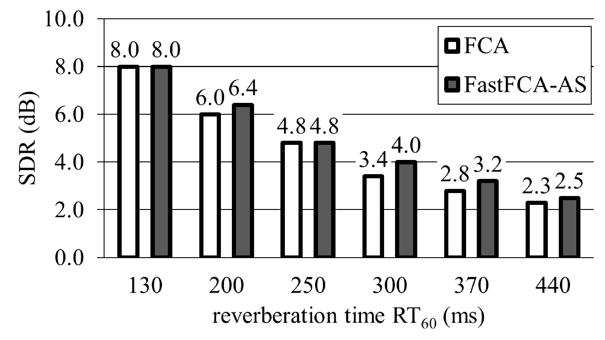
Figure 2 shows the Real Time Factor (RTF) of the parameter estimation averaged over all ten trials and all six reverberation times, and Figure 3 shows the Signal-to-Distortion Ratio (SDR) [10] averaged over all three sources and all ten trials. The proposed FastFCA-AS was over 420 times faster than the FCA with its source separation performance slightly better than the FCA.
6 Conclusions
In this paper, we have proposed the FastFCA-AS, an accelerated algorithm for the FCA. Compared to the conventional FastFCA-TS, the FastFCA-AS has a major advantage of being applicable to not only two sources but also more than two sources.
References
- [1] N.Q.K. Duong, E. Vincent, and R. Gribonval, “Under-determined reverberant audio source separation using a full-rank spatial covariance model,” IEEE Trans. ASLP, vol. 18, no. 7, pp. 1830–1840, Sept. 2010.
- [2] N. Ito, S. Araki, and T. Nakatani, “FastFCA: A joint diagonalization based fast algorithm for audio source separation using a full-rank spatial covariance model,” arXiv preprint, May 2018, arXiv: 1805.06572.
- [3] N. Ito, S. Araki, and T. Nakatani, “FastFCA: Joint diagonalization based acceleration of audio source separation using a full-rank spatial covariance model,” in Proc. EUSIPCO, Sept. 2018 (accepted).
- [4] A.P. Dempster, N.M. Laird, and D.B. Rubin, “Maximum likelihood from incomplete data via the EM algorithm,” Journal of the Royal Statistical Society: Series B (Methodological), vol. 39, no. 1, pp. 1–38, 1977.
- [5] G.H. Golub and C.F. Van Loan, Matrix Computations, The Johns Hopkins University Press, Baltimore, 1983.
- [6] A. Hjørungnes and D. Gesbert, “Complex-valued matrix differentiation: Techniques and key results,” IEEE Trans. SP, vol. 55, no. 6, pp. 2740–2746, June 2007.
- [7] H. Sawada, S. Araki, and S. Makino, “Underdetermined convolutive blind source separation via frequency bin-wise clustering and permutation alignment,” IEEE Trans. ASLP, vol. 19, no. 3, pp. 516–527, Mar. 2011.
- [8] M. Souden, S. Araki, K. Kinoshita, T. Nakatani, and H. Sawada, “A multichannel MMSE-based framework for speech source separation and noise reduction,” IEEE Trans. ASLP, vol. 21, no. 9, pp. 1913–1928, Sept. 2013.
- [9] T. Yoshioka, N. Ito, M. Delcroix, A. Ogawa, K. Kinoshita, M. Fujimoto, C. Yu, W.J. Fabian, M. Espi, T. Higuchi, S. Araki, and T. Nakatani, “The NTT CHiME-3 system: Advances in speech enhancement and recognition for mobile multi-microphone devices,” in Proc. ASRU, Dec. 2015, pp. 436–443.
- [10] E. Vincent, R. Gribonval, and C. Févotte, “Performance measurement in blind audio source separation,” IEEE Trans. ASLP, vol. 14, no. 4, pp. 1462–1469, Jul. 2006.