Incomplete Nested Dissection
Abstract
We present an asymptotically faster algorithm for solving linear systems in well-structured 3-dimensional truss stiffness matrices. These linear systems arise from linear elasticity problems, and can be viewed as extensions of graph Laplacians into higher dimensions. Faster solvers for the 2-D variants of such systems have been studied using generalizations of tools for solving graph Laplacians [Daitch-Spielman CSC’07, Shklarski-Toledo SIMAX’08].
Given a 3-dimensional truss over vertices which is formed from a union of convex structures (tetrahedral meshes) with bounded aspect ratios, whose individual tetrahedrons are also in some sense well-conditioned, our algorithm solves a linear system in the associated stiffness matrix up to accuracy in time . This asymptotically improves the running time by Nested Dissection for all .
We also give a result that improves on Nested Dissection even when we allow any aspect ratio for each of the convex structures (but we still require well-conditioned individual tetrahedrons). In this regime, we improve on Nested Dissection for .
The key idea of our algorithm is to combine nested dissection and support theory. Both of these techniques for solving linear systems are well studied, but usually separately. Our algorithm decomposes a 3-dimensional truss into separate and balanced regions with small boundaries. We then bound the spectrum of each such region separately, and utilize such bounds to obtain improved algorithms by preconditioning with partial states of separator-based Gaussian elimination.
1 Introduction
Linear systems in truss stiffness matrices arise from linear elasticity problems for simulating the effect of forces on geometrically embedded objects [ST08, DS07]. A truss is an undirected weighted graph over vertices which are points embedded in dimensions. We refer to the weights as stiffness coefficients. The associated truss stiffness matrix is a matrix, which can be written as a sum of rank-one positive semi-definite matrices such that each matrix corresponds to an edge in the truss graph.
Graph Laplacian matrices can be viewed as a special case of truss stiffness matrices, in which each vertex is embedded in 1 dimension. 2-dimensional variants have been studied in [ST08] and [DS07]. In this paper, we solve linear systems in truss stiffness matrices of 3-dimensional meshes. These meshes commonly arise from applying finite element methods [SF73] to simulating 3-dimensional physical space in scientific computing and numerical analysis.
Unlike linear systems in graph Laplacians for which nearly-linear time solvers exist (see for example [ST14, KMP10, KMP11, PS14, CKM+14, KS16], etc.), solving linear systems in general truss stiffness matrices can be as hard as solving linear systems over the reals [KZ17], even for 2-dimensional non-planar trusses.
Throughout this paper, we are interested in 3-dimensional trusses with additional geometric structures. Specifically, we assume a truss is a tetrahedral mesh, which can be decomposed into several convex simplicial complexes. In addition, each edge has bounded length and stiffness coefficient, and each tetrahedron has bounded aspect ratio. The aspect ratio of a tetrahedron is the ratio between its volume and the cubic of its diameter. Bounded aspect ratio of simplices is a common criterion in mesh generation [BEG94, Che89, MV92, Rup93].
Existing works which use geometric structures to speed up algorithms are mostly for planar graphs (e.g., [Fre87, Goo95, HKRS97, BKM+11a]). A common structure underlying these speed-ups is the -division. An -division divides a graph into balanced pieces in which only few edges are between any two pieces [Fre87, Goo95, KMS13]. Then divide-and-conquer can be applied. Usually one layer of -division is sufficient for running time speedups [BKM+11a, ŁS11, BENWN14], while recursive -divisions lead to even faster algorithms [HKRS97, BKM+11b, KMS13]. Designing efficient algorithms for 3-dimensional graphs is much harder than in 2-dimensions, even for graphs with bounded genus surface embedded graphs [EN11, BENWN14, BCFN16].
Existing linear system solvers for 3-dimensional tetrahedral meshes are mainly based on nested dissection, which produces a vertex ordering for sparse Gaussian elimination [Geo73, LRT79, MT90, AY10]. The main idea of nested dissection is to recursively compute small separators, which recursively partition a (sub)graph into separate and balanced pieces. Due to small overlaps between any two pieces, Gaussian elimination with this ordering introduces only a small fill-in size. The study of nested dissection, and the prevalence of linear systems in 3-D complexes in turn motivated the study of small separators for 3-dimensional meshes [MT90, MTTV98]. However, the existence of 3-D complexes with no sub-linear sized constant-fraction separators [MT90] means that such algorithms critically depend on the aspect ratios of the individual tetrahedrons.
In addition, support theory has been widely used for solving linear systems in graph Laplacian matrices [ST14, CKM+14] and generalized Laplacian matrices (e.g., connection Laplacians [KLP+16]). Instead of directly solving the original linear system, support theory seeks a sparse preconditioner and iteratively solves a sequence of linear systems (refer to a survey [Axe85]). Both nested dissection and support theory are well-studied techniques in the literature of solving linear systems, but usually they are applied separately.
We design a new approach for solving linear systems in 3-D truss stiffness matrices, by combining the ideas of nested dissection and support theory. We show that the -time11 1 Here we assume that multiplying two matrices needs time , following the convention of nested dissection literature [Geo73, LRT79, GNP94]. We will discuss the running time by using fast matrix multiplication in Appendix B. bound for solving systems on simplicial complexes with bounded aspect ratios [MT90] can be further improved for truss matrices on simplicial complexes formed as a union of convex tetrahedral meshes.
Theorem 1.1 (Informal statement).
Given a linear system in the stiffness matrix of a 3-D truss over vertices satisfying:
- 1.
is a mesh of tetrahedrons formed by a union of convex simplicial complexes with constant aspect ratio each,
- 2.
each edge of has constant length and stiffness coefficient,
- 3.
each tetrahedron of has constant aspect ratio,
and an error parameter , there is an algorithm which outputs a solution of the linear system up to accuracy in time .
Theorem 1.1 improves on Nested Dissection for all . We also show a second result that improves on Nested Dissection even when we allow any aspect ratio for each of the convex structures (but we still require individual tetrahedrons to have bounded aspect ratio and size). In this regime, we improve on Nested Dissection provided .
Our requirements for trusses have more restrictions than the previous nested dissection based algorithms [MT90], which only requires constant aspect ratios for individual tetrahedrons. Our additional restrictions are mainly due to the need to derive spectral bounds for the preconditioner. Assumptions such as bounded edge lengths and stiffness coefficients (in addition to aspect ratios) are also present in previous work by Daitch and Spielman [DS07], which forms the starting point for our key technical results on eigenvalues of 3-D simplicial complexes. Furthermore, the need to maintain null spaces as well as truss structures in intermediate steps of Gaussian elimination places additional requirements on the mesh structure.
Our algorithm can be viewed as incomplete nested dissection. Specifically, for each convex simplicial complex, we compute an -division whose boundaries have nice structures. We then eliminate all interior vertices of the -division, which gives a partial state of Gaussian elimination. To solve the remaining linear system, we simply use the -division boundaries to precondition the intermediate submatrix of the Gaussian elimination as an incomplete Cholesky factorization. Our key technical result shows that the associated stiffness matrix of carefully chosen boundaries has bounded condition number, which may be of independent interest.
This algorithm only relies on the geometric structures of the underlying graphs and good eigenvalue bounds of the associated matrices. Our presentation only represents a basic instantiation of utilizing both geometric structures and spectral ideas to solve linear systems. It is likely that the same techniques can be extended to more linear systems.
Finally, due to reliance on numerical as well as combinatorial structures, our result, as well as previous works on faster linear system solvers for truss matrices [ST08, DS07], are limited to meshes with both bounded side lengths and aspect ratios. This is significantly more restrictive than nested dissection based algorithms that only depend on the aspect ratios of the truss elements. We believe in future works it would be useful to extend our approach to more general cases, and more systematically study the necessity of restricting to such special cases.
1.1 Related Works
| Algorithm | D | Global Req. | Local Req. | Runtime |
| Gaussian Elimination | any | any | none | |
| Fast Inversion [LG14] | any | any | none | |
| Nested Dissection [LRT79] | 2 | any | none | |
| Nested Dissection [MT90] | 3 | any | aspect ratio (AR) | |
| Fretsaw Extension [ST08] | 2 | any | none | unspecified |
| Augmented Tree [DS07] | 2 | stiffly-connected | size, AR, stiffness coefs. | about |
| Theorem 3 | 3 | (convex & AR) | size, AR, stiffness coefs. | |
| Theorem 3.2 | 3 | convex | size, AR, stiffness coefs. |
A comparison of related results and their geometric requirements are given in Table 1. Many geometric restrictions are crucial to designing fast linear system solvers. In addition to requirements on individual truss elements (e.g., bounded aspect ratios, edge lengths and stiffness coefficients), a truss being stiffly connected, defined in [DS07], is important as a global requirement. From a physical view, any deformation of a stiffly connected truss, except a translation and / or a rotation, requires energy. From an algebraic view, the associated stiffness matrix of a stiffly connected truss only has a trivial null space. In our algorithm, we always guarantee that our preconditioner of a convex truss is stiffly connected.
Both direct methods (mainly Gaussian elimination, refer to [Geo73, LRT79, MT90, GNP94, LG14]) and iterative methods (e.g., conjugate gradient, multigrid methods, etc., refer to [Fed64, Axe85, Saa03]) have been widely studied for solving linear systems with additional structures. Combining these two methods has led to fast linear system solvers in graph Laplacians and its generalizations (e.g., [ST14, KMP10, KMP11, PS14, KLP+16, CKP+17, KS16] etc.).
One key idea among these algorithms is incomplete Cholesky factorization. It was used in [KS16] to accelerate Gaussian elimination for graph Laplacian linear systems. Each time the algorithm eliminates a vertex, it sparsifies the partial Cholesky factorization by randomly picking a subset of its nonzeros. In addition, sparsified block Cholesky factorization and multigrid methods were applied in [KLP+16] to solving connection Laplacian linear systems. In [KLP+16], they eliminate a subset of vertices, sparsify its Schur complement (which is an intermediate submatrix of Gaussian elimination, refer to Definition 2.4 for a formal definition) without explicitly computing it, and then repeat this process recursively.
The analyses of both these two papers crucially rely on the fact that graph Laplacian matrices and connection Laplacian matrices are closed under taking the Schur complement. However, this fact does not hold for truss stiffness matrices, for which the Schur complements can be essentially any PSD matrices [KZ17]. The hard instance given in [KZ17] is a 2D non-planar truss. In this paper, instead, we utilize the geometric structures, balanced divisions, and tetrahedral meshes whose tetrahedrons form simplicial complexes and have bounded size and aspect ratio. In this setting we can approximate Cholesky factorization.
One way of measuring the quality of a sparse approximated Cholesky factorization is the relative condition number of the sparse matrix and the original matrix, which determines the number of iterations of preconditioned iterative algorithms. Cheeger’s inequality provides tight bounds on the smallest nonzero eigenvalues of graph Laplacian matrices through sparse cuts in graphs [Chu96]. Extensions to higher-order eigenvalues, connection Laplacian matrices, and simplicial complexes can be found in [LGT14, BSS13, SKM14, PRT16], etc. However, it is unclear whether a Cheeger-type inequality exists for truss stiffness matrices.
1.2 Organization of the Remaining Paper
In Section 2, we give definitions and notations on graphs and linear algebra, and formally define truss stiffness matrices. In Section 3, we present our algorithm for solving linear systems in 3-dimensional trusses and prove our main theorems. Sections 4 and 5 bound eigenvalues of a well-structured truss stiffness matrix which is the key lemma for proving our main results. In Section 6 we show our algorithm for constructing preconditioners, and in Section 7 we show our nested dissection based algorithms for solving linear systems in these preconditioners. Appendix A gives some useful facts on Schur complements, and Appendix B gives our running times parameterized by .
2 Preliminaries
2.1 Tetrahedral Meshes
For a subset , we define the diameter of to be the maximum Euclidean distance between any pair of points in . We define the aspect ratio of to be the ratio between the radius of the smallest ball containing and the radius of the largest ball inscribed in . In mesh generation, aspect ratio is a common criterion for individual elements (see for example [BEG94, Che89, MT90, MV92, Rup93]).
A tetrahedron is the convex hull of four non-coplanar points in . We will specify tetrahedrons in terms of sets of four such points. We refer to a set of tetrahedrons as a tetrahedral mesh.
We say a tetrahedral mesh is a simplicial complex if the intersection of every two tetrahedrons is either empty or a face of both two tetrahedrons. A simplicial complex is convex if the union of the images of its simplices is convex, as defined in [CFM+14].
Definition 2.1.
A tetrahedral mesh is said to be simple iff it is a simplicial complex and every tetrahedron has bounded aspect ratio.
The following definition characterizes rigidity and stiffness of a tetrahedral mesh, which is an adaption of Definition 2.3 in [DS07].
Definition 2.2.
The rigidity graph of a tetrahedral mesh is a graph whose vertices correspond to tetrahedrons and whose edges connect any two tetrahedrons sharing a triangle face. A tetrahedral mesh is stiffly-connected iff (1) its rigidity graph is connected, and (2) for any vertex in the mesh, the rigidity subgraph induced on the tetrahedrons containing this vertex is connected.
We define a bounding box of a convex 3D shape to be a 3D box such that: (1) the box contains all points of this shape, and (2) the volume of the box is same as the volume of this shape up to a constant factor. [BHP01] gives a linear time algorithm which computes a bounding box of a convex shape in 3 dimensions.
Lemma 2.3.
(Lemma 3.6 of [BHP01]) Given a 3D convex shape, one can compute in linear time a bounding box of this shape.22 2 The lemma statement in [BHP01] gives a bound related to the minimum-volume bounding box of the input shape, but their proof uses the volume of the shape as a lower bound of the volume of . Moreover, the aspect ratio of the bounding box is same as the aspect ratio of the given shape up to a constant factor.
2.2 Vectors and Matrices
Given a vector , for , we denote the th entry of , and we denote the subvector whose entries are . The Euclidean norm of is defined as .
Given a matrix , for , we denote the th entry of . A square matrix is a positive semi-definite matrix (PSD) iff for every vector we have . We denote the smallest nonzero eigenvalue of .
For two symmetric matrices , we say iff is PSD. We define the condition number of relative to , denoted by , to be
In addition, we define Schur complements which arise from the process of Gaussian elimination.
Definition 2.4 (Schur complement).
Let be a partition of the indices of a square matrix so that where are block matrices, the Schur complement of onto is
We will use the following fact of Schur complements.
Fact 2.5 (Lemma 4 of [RTL76]).
Let be a symmetric matrix, the th entry of the Schur complement only if there exists a sequence of indices such that all are nonzero.
Fact 2.6.
Let be a symmetric PSD matrix and be its Schur complement.
- 1.
is a symmetric PSD matrix.
- 2.
.
2.3 Solving Linear Systems
Our algorithm combines two of the most important tools for solving linear systems: Nested dissection and preconditioning. Below, we give a brief introduction to some of the central results on these techniques.
Classic results due to Lipton, Rose, and Tarjan [LRT79], and Miller and Thurston [MT90] combine to show that linear systems arising from simple tetrahedral meshes (see Definition 2.1) can be solved in time. These results concern linear equations in an matrix where the indices can be embedded as points that form the vertices of an explicitly given, simple tetrahedral mesh, and is non-zero only if the vertices and share an edge in the tetrahedral mesh.
Theorem 2.7 (Nested dissection [MT90]).
Let be a symmetric matrix defined on a simple tetrahedral mesh. A Cholesky factorization can be computed in time , in which is a permutation matrix and is a lower triangular matrix with nonzero entries. As a result, a linear system in can be solved in time by Gaussian elimination.
Theorem 2.7 can be extended to a block matrix where is a constant positive integer. Each vertex of the underlying graph corresponds to indices of . In addition, the block corresponding to the column indices for vertex and the row indices for should be non-zero only if the vertices and share an edge in the tetrahedral mesh, or if , i.e. when the block is on the diagonal.
The Nested Dissection algorithm relies on invoking separators recursively. A separator is a set of indices such that the remaining indices can be partitioned into two sets and such that every entry with and has . Furthermore, we guarantee that the partition is roughly balanced, for example, each of and contains no more than indices. Nested Dissection recursively repeats the partitioning process on the union of each subset and the separator itself, that is, and . Given such a recursive partition scheme, we reorder the indices of the matrix so that the indices in the separator are eliminated last, and we then order the indices in and recursively in a similar way. We perform Gaussian elimination on the matrix according to this ordering, which only introduces a small fill-in size and few multiplication counts. This approach also works for eliminating a subset of the variables, resulting in a Schur complement on the rest.
Both the running time and representation cost of nested dissection algorithms are bottlenecked by the costs of the top-level separators. In Algorithm 1 TrussSolver, we will utilize improved running time bounds for nested dissection when better separators exist. The following lemma characterizes the performance of Nested Dissection given better top-level separators.
Lemma 2.8.
Suppose we have a recursive separator decomposition of a simplicial complex with bounded aspect ratio tetrahedrons such that:
- 1.
the number of leaves, and hence total number of recursive calls, is at most .
- 2.
each leaf (bottom layer partition) has at most tetrahedrons.
- 3.
each top separator has size at most .
Then we can find an exact Cholesky factorization of the associated stiffness matrix in time , and the total resulting fill-in is .
We give a proof of the above lemma in Section 7.1, which is an adaption of the analysis in [LRT79] We remark that the algorithmic realization of this can be viewed as utilizing the nested dissection algorithm 2.7 to complete this structure into a full separator tree.
Last but not least, we state the following theorem for preconditioned conjugate gradient, which will be used in bounding the running time of our algorithm.
Theorem 2.9 (Preconditioned conjugate gradient [Axe85]).
Let be two symmetric positive semidefinite matrices and let . Each iteration of the preconditioned conjugate gradient multiplies one vector by , solves one linear system in , and performs a constant number of vector additions. For any , the algorithm outputs an satisfying in such iterations.
We remark that while there are settings where the convergence of preconditioned conjugate gradient is numerically unstable, the eigenvalue-based bound that we utilize here is stable once the solves involving have polynomially small errors.
2.4 Truss Stiffness Matrices
We extend the definition of 2-dimensional truss stiffness matrices from [DS07] (see Definition 2.1 and 2.2) to 3 dimensions.
Definition 2.10 (3-dimensional truss).
3-dimensional truss is given by
- •
A set of vertices embedded at distinct points
- •
A mesh (i.e. set) of tetrahedrons , each specified in terms of four vertices, i.e. we identify tetrahedron with both four vertices and the convex hull of .
- •
A set of edges which is exactly the set of pairs of vertices that appear in some tetrahedron together. Each edge represents a straight idealized bar between vertex points and .
- •
A function , which assigns a stiffness coefficient to each edge . The stiffness coefficient represents the stiffness of the idealized bar corresponding to edge .
Definition 2.11 (Truss stiffness matrix).
Let be a 3-dimensional truss. For each edge , we define an edge vector with 6 nonzero entries:
The stiffness matrix of the truss is defined as
In general, solving linear systems in truss stiffness matrices can be as hard as solving linear systems in real matrices [KZ17].
In this paper, we study 3D trusses with some additional geometric structures. These structures enable us to design linear system solvers that run much faster than solvers for general simple tetrahedral meshes.
Definition 2.12.
We say a 3D truss is edge-simple if its tetrahedral mesh is simple and every tetrahedron has bounded edge lengths and stiffness coefficients (i.e. both are bounded above and below by constants).
Definition 2.13.
We say a 3D truss is convex edge-simple if it is edge-simple, and its tetrahedral mesh is convex.
3 Algorithm Overview
In this section, we present our algorithm for solving linear systems in stiffness matrices of edge-simple 3D trusses. Our first main result concerns trusses formed by combining convex edge-simple trusses, each with constant aspect ratio upper bounded by some arbitrarily large but fixed constant.
Theorem 3.1.
Given an edge-simple 3-D truss with vertices, formed from a union of convex edge-simple trusses each with aspect ratio at most 33 3 A slightly modified analysis extends this result to allow each individual truss has aspect ratio , where is the number of vertices of the th individual truss., and an error parameter , there is an algorithm which solves a linear system in the corresponding stiffness matrix up to accuracy in time .
This theorem is appealing because in many modeling applications, only large constant aspect ratios are needed for individual convex parts that are being combined. In Theorem 3, we see that the performance degrades smoothly towards the running time of Nested Dissection as approaches .
Our second main result deals with the case when we allow a truss formed from convex edge-simple trusses, each of which may have arbitrarily large aspect ratio.
Theorem 3.2.
Given an edge-simple 3-D truss with vertices, formed from a union of convex edge-simple trusses, and an error parameter , there is an algorithm which solves a linear system in the corresponding stiffness matrix up to accuracy in time .
We remark that the geometric assumptions of Theorem 3.2 are in many ways fairly weak. We need the individual truss tetrahedrons to have small aspect ratio, but each of the convex edge-simple trusses may overall have a wide range of shapes: It can form a ball, a pancake, or even a very long beam with arbitrarily large aspect ratio. The dependence on is fairly bad and has not been carefully optimized, meaning currently that only about convex edge-simple trusses can be combined while still achieving a speed-up over nested dissection. Even so, this allows the construction of some shapes with genus up to .
Fast matrix multiplication can be used in our algorithm, as well as earlier routines. In accordance with previous works on nested dissection, and to simplify presentation, we assume (the matrix multiplication constant) throughout our calculations. However, in Appendix B, we also give the -dependent bounds. Assuming as in [LG14], the bounded aspect ratio case from Theorem 3 takes time , while the arbitrary aspect ratio case from Theorem 3.2 takes time . In both cases the running times are less than the bound obtained by plugging into 3-D nested dissection.
Our algorithm pseudocode is stated in Algorithm 1. Note this algorithm proves both Theorem 3 and 3.2. Theorem 3 is a special case where in line 4.
3.1 Main Ideas
Both our main theorems are based on speeding up Nested Dissection by combining it with preconditioning and iterative solvers. In Section 2.3 we gave a brief outline of Nested Dissection. In classical Nested Dissection, the main bottleneck that constrains the running time of the algorithm is the process of applying Gaussian elimination to the few separators in the top levels of the separator tree, after having eliminated all the matrix indices at lower levels. The intermediate matrix that arises during Nested Dissection after eliminating the indices at lower levels is in fact the Schur complement onto the separators at top levels.
Our central idea that gives us an advantage over Nested Dissection is that: the outer boundary of tetrahedrons of a single convex edge-simple truss44 4 It can be a subset of one of the input individual convex edge-simpletrusses. with small aspect ratio is a good preconditioner for the Schur complement of the whole truss onto the boundary.
By forcing Nested Dissection to use these outer boundaries of individual convex edge-simple trusses as the top-level separator, we get a separator which has a good sparse preconditioner. Fortunately, we can also ensure that this top-level separator has a small size.
The phenomenon that the boundary itself is a good preconditioner for the Schur complement onto the boundary has a natural interpretation based on structural mechanics. The quadratic form associated with the Schur complement corresponds to the energy associated with deforming the whole truss by squishing or stretching the boundary vertices while leaving the interior intact and finding the positions of the interior vertices that minimize the overall energy. We show that this energy is not much more than the energy that arises from applying the same deformation to just the boundary tetrahedrons after deleting the interior vertices.
This means that we can speed up the process of applying the inverse of the Schur complement onto the boundary, which is the bottleneck of nested dissection. We avoid directly inverting the Schur complement by instead solving a linear system in the Schur complement using the boundary itself as a preconditioner in preconditioned conjugate gradient. Because the boundary is much sparser than the Schur complement, and has much fewer tetrahedrons than the initial mesh, we significantly reduce the running time.
How good a preconditioner the boundary is for the Schur complement depends on the number of tetrahedrons in the initial convex mesh. If the mesh is large, then the preconditioner is worse in the sense that solving an associated linear system is time-consuming, but the gain from hollowing out the mesh is relatively larger, because the number of tetrahedrons on the surface is relatively smaller. Ideally, we want to balance these two phenomena against each other. We can ensure a good trade-off between these two effects by first dividing very large convex trusses into smaller chunks before hollowing out these chunks and using the resulting boundaries, which now look somewhat like a Swiss cheese, as a preconditioner.
All together, this approach of partitioning, hollowing out, preconditioning, and using Nested Dissection gives us Theorem 3.
If the aspect ratios of individual convex trusses are allowed to be extremely large, so that the trusses can be very thin, then we cannot gain much by hollowing out the trusses. However, if an individual convex truss has large aspect ratio, then we can get good separators for Nested Dissection by slicing the truss along its longest dimension. Combining this observation with our preconditioning approach, we are able to obtain Theorem 3.2, which has no requirements on the aspect ratios of each of the trusses we are combining. Unfortunately, leveraging both the preconditioning behavior and the existence of good separators for individual large aspect ratio trusses requires fairly technical work, which currently introduces a bad dependence on in this version of our main result.
3.2 Bounding Eigenvalues of an Edge-Simple and Stiffly-Connected Truss
Our main structural results are bounds on the condition number of the stiffness matrix of a edge-simple and stiffly connected (see Definition 2.2) simplicial complex. As each vertex is involved in at most a constant number of tetrahedrons, we can easily obtain bounds on the maximum eigenvalue.
Thus, our main technical contribution is a lower bound on the minimum non-zero eigenvalue of the stiffness matrix of a 3D edge-simple truss. We state the explicit bound in Lemma 3.3. Such a bound is analogous to the bound on minimum eigenvalues of a path in a graph.
Lemma 3.3.
Let be an edge-simple and stiffly-connected 3D truss. Let be the number of vertices of and be the diameter. Let denote the associated stiffness matrix. Then, and .
Our proof is heavily motivated by the Path Lemma by Daitch and Spielman [DS07], which bounds the minimum non-zero eigenvalue of the stiffness matrix of a path of triangles in 2D. We start by shifting all the tetrahedrons by the normals w.r.t. a particular centering tetrahedron, which in effect projects away the coordinates from the null space. Then we lower bound the minimum dot-product of a quadratic form in terms of the pairwise differences among these tetrahedrons. However, our calculations result in an exponential factor loss depending on the “hop distance” between the first and last tetrahedrons. This is due to the accumulation of rotational operators, which we need to treat as matrices instead of simple rotations.
We are not sure whether this exponential increase is simply due to an algebraic artifact in our proof. To circumvent it, we instead show that there exists a particular centering where a pair of close-by tetrahedrons are placed apart. This proof relies on analyzing the “average behavior” of all centerings globally. It once again relies on treating the initial rotations and projections as linear operators, and working directly with the singular values of these projection operators.
3.3 Proving the Main Result for Small Aspect Ratio Truss Unions
To accelerate Nested Dissection, we need to find a set of balanced separators that are small and whose Schur complements have good sparse preconditioners.
To build these good separators, motivated by -divisions, we divide each of the small-aspect ratio trusses in our union of trusses into smaller chunks, such that the boundary of each chunk is a good preconditioner of the Schur complement onto that boundary. The union of all these boundaries is called a hollowing. To create a hollowing, we fix two parameters: a bounding box that determines the directions of each smaller chunks of the hollowing, and a size parameter that controls the size of the smaller chunks. We call each smaller chunk as a region.
Definition 3.4 (-hollowing).
Given a convex edge-simple3D truss , a bounding box of , and a parameter where is the aspect ratio of , a -hollowing of is another edge-simple 3D truss such that, , , and is the subset of that arises from edges in , while is just the restriction of to . I.e. edges maintain the same stiffness factors as in . Also
- 1.
contains points. consists of disjoint chunks, each of which has vertices and is incident to vertices of .
- 2.
for every plane whose normal vector has angle with the longest direction of , the number of tetrahedrons in intersected by is
- 3.
.
The next lemma describes the performance of algorithm Hollow, Algorithm 2 in Section 6, that we use to compute a -hollowing of a convex edge-simple truss.
Lemma 3.5.
Given a convex edge-simple 3-dimensional truss with vertices, a bounding box of , and a positive integer such that the aspect ratio of is at most , the algorithm returns a -hollowing of , and runs in time .
Proof of Theorem 3.
Let be a edge-simple 3-D truss with vertices, formed from a union of convex edge-simple trusses, say , each with aspect ratio at most . For each , let be the number of vertices of , and define . In Algorithm 1, for each , we compute a -hollowing, where is a bounding box of . By Lemma 2.3 and 3.5, the total running time here is . In each -hollowing region, we eliminate its interior vertices in total time
The Schur complement onto the boundaries has
nonzeros. We then run preconditioned conjugate gradient (PCG) to solve the linear system in the Schur complement by preconditioning it via the union of the -hollowings, say . Note by Jensen’s inequality, has size
Before running PCG, we compute a Cholesky factorization of by nested dissection. According to Theorem 2.7, the running time is , and the fill-in size is . By Definition 3.4, the condition number is . According to Theorem 2.9, the number of PCG iterations is at most to output a solution up to accuracy . In each PCG iteration, we do a matrix-vector multiplication with the Schur complement in time , and solve a linear system in in time . Thus the total running time is . ∎
3.4 Proving the Main Result for All-Aspect Ratio Truss Unions
We extend our result to cover the case when the union of convex edge-simple trusses also include trusses with arbitrarily large aspect ratios. The lemma below shows that large aspect ratio implies the existence of good plane separators, which is proven in Section 7.
Lemma 3.6.
Given a convex edge-simple 3D truss with aspect ratio at least , say, , and its bounding box . Let be a unit vector along the longest direction of , and let be a unit vector with . Then every plane orthogonal to intersects at most tetrahedrons.
The above lemma tells us that a single convex edge-simple truss with large aspect ratio has a good plane separator. It turns out that even if we have many such trusses whose longest dimension may point in different directions, and we have hollowed-out trusses from small aspect ratio parts, we can still find a single plane that acts as a reasonably good separator for all of these trusses at the same time. This is captured by the following lemma, which is obtained by instantiating Lemma 7.3 with and .
Lemma 3.7 (Combining Separators).
Given a edge-simple 3D truss , which is a union of convex edge-simple trusses with up to vertices in total. Let be a truss by selectively computing -hollowings of some of the pieces with parameter
There exists a randomized algorithm which with high probability returns a vertex ordering so that a complete elimination of has size , and takes time to compute.
The algorithm that achieves Lemma 3.7 is Algorithm 4 ConvexTrussUnionND in Section 7. Given these lemmas, we can now sketch a proof of Theorem 3.2.
Proof of Theorem 3.2.
We bound the running time of Algorithm 1 TrussSolver with the preconditioner and nested dissection constructed as per Lemma 3.7.
Since all the hollowings involve pieces with , Definition 3.4 gives a bound of on the condition number, and in turn a bound of on the number of PCG iterations via Theorem 2.9. Furthermore, similar to the proof of Theorem 3, the Schur complement of onto the elements of has size , and computing them by eliminating all interior vertices of our hollowings takes time .
4 Bounding the Smallest Nonzero Eigenvalue of a edge-simple Truss
In this section, we prove Lemma 3.3, which lower bounds the smallest nonzero eigenvalue of a edge-simple 3D truss. We restate Lemma 3.3 in the following.
Lemma 3.3.
Let be an edge-simple and stiffly-connected 3D truss. Let be the number of vertices of and be the diameter. Let denote the associated stiffness matrix. Then, and .
4.1 Main Ideas
The proof of Lemma 3.3 is an extension of the path support lemma by Daitch and Spielman [DS07]. That proof relies on recentering a vector , which is a unit vector orthogonal to the null space, with respect to the a single face by transforming it along the null space of .
Let be a 3D stiffly-connected truss over vertices. The null space of the stiffness matrix of can be characterized as:
- 1.
, , : for each , the corresponding 3-dimensional vector ( and ) has 1 for its -coordinate (-coordinate, and -coordinate, respectively) and 0 for the other two coordinates.
- 2.
, , : fix an arbitrary index , for each :
Also, as many of our arguments are symmetric across dimensions, we will use , and to represent symmetric indexing over the dimensions, or pairs of dimensions respectively. Finally, as centering and exploring a simplicial complex from a particular triangle introduces an ordering on the tetrahedrons, faces, and edges, we will define our edges, triangles, and tetrahedrons as ordered tuples:
- 1.
Edges: ,
- 2.
Triangles: we denote these as . Here means the edge .
- 3.
Tetrahedrons: an ordered 4-tuples of pairwise adjacent points, . Here means the (triangle) surface , and means the edge .
With these notations in mind, we can center a vector w.r.t. a particular (oriented) triangle surface . This can be viewed as an extension of the centering lemma in [DS07]. We prove the following Lemma in Section 4.2.
Lemma 4.1.
Given a stiffly-connected, edge-simple truss , let be a vector orthogonal to the null space of its stiffness matrix. For each oriented triangle , there exists a (unique) vector with scalar shift parameters , , :
| (1) |
satisfying:
- 1.
the plane containing the points is parallel to the plane containing .
- 2.
The edge is parallel to the edge .
Daitch and Spielman then showed that with any centering, the value of is lower bounded by the sum of a series of shifted values, or in simpler terms, the norm of for some edge . However, our extension of this bound (which we will describe next in Lemma 4.4) to the 3-D case has an exponential dependency on the distance in tetrahedrons between and . As a result, we first show the existence of a good centering, namely one where there exist an edge close to whose endpoints are far apart. This notion of distance can be defined in terms of ‘hop count’ of tetrahedrons.
Definition 4.2.
The tetrahedron-distance between a pair of objects and in a simplicial complex is the shortest sequence of tetrahedrons
such that , , and for all , and share a triangle face.
We remark that because all edges and angles are within some constant range, this combinatorial distance is within constant factors of the Euclidean distance of the associated points. However, we will not make use of this connection.
Lemma 4.3.
Given a stiffly-connected, edge-simple truss with vertices and diameter , let be a unit vector orthogonal to the null space of the stiffness matrix of . There exists an oriented triangle and a pair of points within tetrahedron-distance of satisfying:
We prove this lemma in Section 4.3.
We can then check, via an argument similar to [DS07], that such a centering and distance pair implies a large quadratic form. The following lemma will be proved in Section 5.
Lemma 4.4.
Given a stiffly-connected, edge-simple truss with stiffness matrix , an oriented triangle , and a pair of points within tetrahedron-distance of , we have
4.2 Centering a Vector (Proof of Lemma 4.1)
To prove Lemma 4.1, we define the following operation. Let be any fixed plane in and let . We define to be the vector obtained by first projecting onto plane and then rotating the projected vector on the plane counterclockwise by . The following claim shows that can be written as a linear combination of .
Claim 4.5 (Rotation matrix).
Let be any fixed plane in , and let be its normal vector. Then,
Proof.
Let
be the rotation matrix which rotates a vector on the plane counterclockwise by . Then,
We can check that . It implies that .
On the other hand,
Thus, the claim holds. ∎
Claim 4.6.
Let be a nonzero vector. Then matrix
has rank 3.
Proof.
The 2-by-2 bottom left submatrix has determinant . If , then clearly has rank 3 and we have done; otherwise, the 3rd and the 4th rows are independent.
Now it suffices to show that the 2nd row is independent of the 3rd and the 4th rows. Assume by contradiction, suppose
By solving the last two equations, we get and . Plugging these values into the 1st equation, we have , which contradicts that . ∎
Proof of Lemma 4.1.
Let be the normal vector of the plane containing , that is,
We first show that there exist such that the vector
satisfies the first condition. It suffices to show that the following linear system has a solution for real numbers ’s:
Rearrange it and write it in matrix form:
It suffices to show that the coefficient matrix has rank 2.
Assume by contradiction, there is some such that
It equals to
Let . Since vectors are not parallel, we have . Besides, . Write the above equation in matrix form:
By Claim 4.6, the coefficient matrix has rank 3, which implies that . It contradicts that .
Then we show that there exist such that
satisfies both conditions.
Let be the plane containing . Let satisfy
Then, there exists an appropriate multiplier such that the vector
is parallel to . Besides, since both and are parallel to the plane , the vector is parallel to the plane .
4.3 Existence of Good Centering (Proof of Lemma 4.3)
In this section we prove Lemma 4.3.
The proof is by contradiction. We assume that for every centering at a triangle , for every pair within tetrahedron-distance 3 of satisfies
| (3) |
where for a sufficiently large constant .
Recall that in Lemma 4.1, for each centering at , we define 3 scalar coefficients
for the null space vectors in Equation (1). We will write the vector containing these 3 coefficients as .
To prove Lemma 4.3, we need the following lemma. It says that, under the assumption in Equation (3), the difference between the coefficient vectors w.r.t. to two close centering triangles is small.
Lemma 4.7.
Assume that for every centering triangle and every pair of points within distance of satisfies Equation (3). Then for every pair of centering triangles and within constant tetrahedron distance to each other, we have
The next lemma implies that: for any two vertices such that each is centered w.r.t. a triangle close to itself, the difference between the two centered vertices is small.
Lemma 4.8.
Let be two arbitrary vertices of . Let () be a triangle containing (and , respectively). Under the assumption in Equation (3), we have
Proof.
Let be a shortest path from to . Note . Let be a triangle next to for . The path from vertex , centered at , to vertex , centered at , can be expressed as the following:
Taking norm on both sides and applying the triangle inequality, we an bound the norm of the LHS by the sum of norm of each term in the RHS.
Now we prove Lemma 4.3.
Proof of Lemma 4.3.
For each vertex , let denote an arbitrary triangle next to vertex . We can write vector as
| (5) |
where
Note that the last two terms of Equation (5) are in the null space of . Thus,
On the other hand, by the triangle inequality,
We apply Lemma 4.8 to the first term, and apply Equation (4) (which is true for any two close centering triangles) times for the second term:
By our choice of for a sufficiently large constant , we get a contradiction. ∎
It remains to prove Lemma 4.7. For it, we define a matrix w.r.t. a given vector :
We will use the following properties of .
Lemma 4.9.
For the matrix as defined in Equation (4.3), its singular values are , and its null space is multiples of the vector .
Proof.
For any vector , the cross product . That is, is the vector obtained by:
- 1.
First projecting onto the plane with normal vector , say , and
- 2.
then rotating the projected vector on the plane by counterclockwise.
From this description, we can infer that
and any vector orthogonal to is on this plane . Such vectors are not affected by the first step projection, and their lengths are not changed by the subsequent rotation. This means for such vectors we have . Thus, the singular values of are 1,1,0. ∎
Lemma 4.10.
If and are vectors with length at least such that the angle between them is , then the matrix
is full rank, and has minimum eigenvalue at least .
Proof.
Let be a unit vector. Decompose :
where , is a unit vector orthogonal to , and is a unit vector orthogonal to . Then,
By Lemma 4.9, and . Thus,
The second equality is due to that is a unit vector.
Therefore,
implies that , and thus the matrix has full rank. ∎
Equipped with the above lemmas, we prove Lemma 4.7.
Proof of Lemma 4.7.
Let and be two triangle centerings for which there exist two edges belong to same tetrahedron, say , such that vertices are all within tetrahedron-distance constant of both and .
Recall is defined in Equation (1). Subtracting
from the corresponding equation for gives:
Plugging in the definition of :
Subtracting this equation from centering triangle in turn cancels the term on the RHS, giving:
Together with the corresponding equation for ,
Multiplying on both sides gives:
Solving the above linear equations and taking norm on both sides:
Applying Lemma 4.9 and 4.10 on the first two terms, and applying the triangle inequality and the assumption in Equation (3) give:
∎
5 Proof of Path Lemma
We now prove Lemma 4.4, which lower bounds the quadratic form of an edge-simple and stiffly-connected truss stiffness matrix by the distance between two centered points. As we now only deal with a single centering in this section, we will drop this superscription for simplicity and relabel all indices w.r.t. this centering. Our relabeling is similar to that in [DS07].
5.1 Relabeling Tetrahedrons and Vertices
Fix an arbitrary tetrahedron, say , and we center the vector w.r.t. one of the triangle faces of as in Lemma 4.1. Use as root, we run breadth-first-search (BFS) in the rigidity graph (refer to Definition 2.2) of , and relabel the tetrahedrons of according to this BFS ordering. For example, the neighbor tetrahedrons of are labeled as . Let be the corresponding BFS tree in which each node represents a tetrahedron in .
Based on , we relabel the vertices of as follows. We label the vertices of by in an arbitrary order. Each child of (and subsequent recursions) shares a triangle face with their respective parent tetrahedron and thus only requires us to label one vertex per child tetrahedron, which can be labeled according to the BFS ordering.
For each newly labeled vertex , we use to denote the tetrahedron encompassing the and its parental face. Besides, we use a 3-dimensional vector to consist of the indexes of the parental face sorted in ascending order, and is assumed that indexing this vector is implicitly modulo 3. Then, . For completeness, we define . See Figure 1 for an example.

5.2 Distance between Local Minimizers and the Centered Vectors
Let be a unit vector which is orthogonal to defined at the beginning of Section 4.1. By Lemma 4.1, there exist scalars such that the vector
satisfies:
- 1.
the plane containing is parallel to the plane , and
- 2.
is parallel to .
We drop the superscription when the context is clear.
For each , we define a 3-dimensional vector . is a vector on the plane of and minimizes the energy / quadratic form, suppose both are fixed. That is,
| (9) |
For each , is a vector which minimizes the energy / quadratic form, suppose all the three points of are fixed. That is,
| (10) |
We then define the distance between each local minimizer and the centered vector . Specifically,
This definition intermediately gives that ,
| (13) |
Note that equation (13) describes the net stress on an edge.
Let
Let such that for each ,
where and denotes accessing specific dimensions of vectors modulo 3. Then we define
Similarly, for , let
and
| (14) |
where with
Claim 5.1.
| (15) |
Proof.
Claim 5.2.
Proof.
We first show that the diagonals of are equal to .
Similarly, we have
Then, we show that the off-diagonals of are 0.
The last equation is due to the 3 columns of the matrix are linearly dependent. Similarly,
This completes the proof. ∎
Plugging the above equations into the definition of ’s gives:
Claim 5.3.
For each ,
5.3 Bounding the Norm of in terms of ’s
Rearranging the above equation gives that for each ,
| (16) |
Our goal is to express each as a function of . If each term in the right hand side of Equation (16) satisfies
for some and , then we can substitute it by Equation (16) with the left hand side being . The substitution terminates when the right hand side term becomes .
Claim 5.4.
Let () be a term appearing in the right hand side of Equation (16). There exist satisfying
Proof.
Without the loss of generality, assume . If , then ; if , then . The remaining proof focuses on .
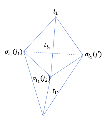
Let be the other vertex in tetrahedron . Let be the parent of in the BFS tree . , and the two tetrahedrons and share a triangle face containing vertices . See Figure 2. If , then
Otherwise , we prove the statement by case analysis.
Case 1. .
By our labeling rules, vertex is the one with the maximum index among all the vertices of and it is contained in the triangle shared by and .
Thus, and
for some .
Case 2. .
Then, and
.
Note .
By induction on the tetrahedron index , we can see that there exist satisfying
.
∎
We use a recursion tree to express the process of recursively substituting via Equation (16). The root of is , and each node of represents a term which is substituted at that point. The leaves are , which equals by Equation (5.2).
Claim 5.5.
The number of nodes in the recursion tree is at most .
Proof.
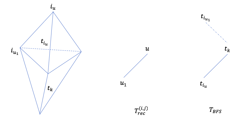
Since is a binary tree, it suffices to prove that the height of is at most . For each non-leaf node of , let be a child of . According to Equation (16) and our labeling rules, is a vertex in tetrahedron and . Let be the tetrahedron such that and share a triangle face containing vertices . Then in , is the parent of . Since , in , the depth of is smaller than the depth of . See Figure 3. It implies that the height of is at most the height of , which is at most .
∎
At each node of the recursion tree , by applying Equation (16) with the left hand side being , we introduce a term related to . For each non-root node , denote the parent of in . Let be the path from the root node to node in . For each non-root node , define
| (17) |
For root node , define . By recursively applying Equation (16), we get
where . By the triangle inequality and the multiplicative inequality of 2-norm,
| (18) |
We bound for each non-root node by the following claim.
Claim 5.6.
Let be the maximum edge length, and let be the minimum tetrahedron volume. Define , which is a constant by our assumption that all tetrahedrons have constant aspect ratios and all edge lengths are constant. For each non-root in , .
Proof.
Let be the vertices along the path . By the proof of Claim 5.5, the length of is at most . Let and for each . By Equations (17), (14), and (15),
Recall that from Claim 5.1,
which is equal to the volume of the tetrahedron generated by vectors , and . Similarly, equals to the volume of the tetrahedron generated by vectors , and . Thus, by our definition ,
Thus,
∎
5.4 Bounding the Quadratic Form
Claim 5.7 (Lemma 3.7 of [DS07]).
Under the assumption: the angle between and is in the range for some constant . For any fixed unit vector ,
Claim 5.8.
Under the assumption of constant edge lengths: for each , the determinant of the matrix:
Furthermore, for any fixed unit vector , for each ,
Proof.
The determinant of matrix is the signed volume of tetrahedron , which is constant by our assumption.
We claim that for any unit vector , there exists some such that . Assume by contradiction, for every we have . This means that all three vectors are between two 2D planes with distance and orthogonal to . This contradicts the assumption that the volume of tetrahedron is constant.
Thus, we have
∎
Therefore,
Applying the Cauchy-Schwarz inequality on the above equation and Equation (19) gives the path lemma.
6 Computing a -Hollowing of a Convex Edge-simple Truss
In this section, we present Algorithm 2 Hollow, which is used as a subroutine for line 6 of Algorithm 1 TrussSolver. The input of Algorithm 2 consists of a convex edge-simple 3D truss , a bounding box and an integer parameter . The algorithm outputs a -hollowing of . We can check that the algorithm terminates in time . These together prove Lemma 3.5.
Given that each individual tetrahedron has constant volume and constant aspect ratio, the following observation converts counting the number of tetrahedrons in a truss intersecting a 2D plane into the intersection area of this truss and the plane.
Observation 6.1.
Let be a convex edge-simple 3D truss, and let be a 2D plane. Let be the intersection area of and . Then the number of tetrahedrons in intersecting is upper bounded by .
Proof.
Since every individual tetrahedron in has constant volume and constant aspect ratio, a tetrahedron of intersects only if all points of this tetrahedron is within some constant distance of . The number of tetrahedrons of intersecting can be upper bounded by the volume within some constant distance to . Thus, the number of tetrahedrons of intersecting is at most . ∎
6.1 Bounding the Size of
In this section, we show that , computed by Algorithm 2, has a small size. That is, satisfies the first condition of the -hollowing definition in Definition 3.4.
Note in Algorithm 2 line 1, the bounding box is divided into small cubes of volume each. We call a small cube as a region. The tetrahedrons in a region are the tetrahedrons of which intersect a single small cube. A tetrahedron can appear in at most eight regions.
The following lemma upper bounds the number of tetrahedrons of in each region.
Lemma 6.2.
Given a convex edge-simple 3D truss of vertices, a bounding box and a positive integer , let returned by Algorithm 2. Then, has at most tetrahedrons.
Note the shortest side length of the bounding box of is at least . The requirement guarantees that the shortest side length is at least so that an -division exists.
Proof.
Note has regions. It suffices to show that each region of has at most tetrahedrons.
Let be a region of . A tetrahedron of belongs to region if either this tetrahedron is within constant distance to the boundary of , or this tetrahedron is within constant distance to the part of the boundary of that’s contained in . Since every tetrahedron of has constant volume and aspect ratio, the number of tetrahedrons within constant distance to the boundary of is . It remains to bound the number of tetrahedrons within constant distance to the boundary of that’s contained in .
Define . Since both and are convex, is convex. Let the surface area of a shape. By Observation 6.1, the number of boundary tetrahedrons of contained in is .
Let be the smallest ball containing . Since is a cube, we have
So it suffices to show . We do so by giving a one-to-one mapping of every point from the surface of onto .
Let which maps each face of to a subset of the surface of , defined as follows. Consider a face of , say , with vertices in a clockwise order. Let be the plane containing . cuts into two parts, let be the part of the smaller volume (break a tie arbitrarily), aka the sphere cap generated by the plane .
For each , let be the plane orthogonal to that passes through and (if , then the intersection line is ). Let be the point of intersection of the surface of with the planes and (if , then is the intersect vertex of and the surface of ).
We define to be the surface of enclosed by . See Figure 4 for an example.

For each face of , the orthogonal projection of onto the plane is . Thus
In addition, since is convex, for any two distinct faces and , and are also disjoint. So we have
Combining this with then completes the proof. ∎
6.2 Bounding the Number of Tetrahedrons in Intersecting with a Plane
In this section, we show that , computed by Algorithm 2, has a small overlap with any plane whose normal vector has an angle between with the longest direction of . That is, satisfies the second condition of the -hollowing definition in Definition 3.4.
Lemma 6.3.
Given a convex edge-simple 3D truss of vertices, a bounding box and a positive integer , let returned by Algorithm 2. Let be a unit vector such that the angle between and let the angles with the three directions of the box (normals to its faces) be , for some . Then, the number of tetrahedrons in which intersect any plane orthogonal to is at most
Without loss of generality, we assume that the bounding box is axis-parallel, that is, the sides of are parallel to the three axes: the axis, the axis and the -axis. We say an axis-paralleled box has side lengths , if the sides parallel to the -axis have length , the sides parallel to the -axis have length , and the sides parallel to the -axis have length , respectively.
To prove Lemma 6.3, we need the following claim, which bounds the intersection area of a 2D plane and a 3D box.
Claim 6.4.
Let be a 3D axis-parallel box of side lengths . Let be a unit vector such that the angle between and the -axis (the -axis, and the -axis) is (, respectively). Suppose . Then the intersection area of any 2D plane orthogonal to and the 3D box satisfies
Proof.
Since the three terms in the right hand side are symmetric, we only prove can be upper bounded by the first term and the other two follow in a similar way.
Let be the two faces of which are orthogonal to the -axis, without loss of generality, assume has a smaller -coordinate.
If intersects neither nor , then the volume of is equal to .
If intersects say with line , see Figure 5, then we draw a line going through point and parallel to the -axis, which intersects face at point , similarly we draw a line going through point and parallel to the -axis, which intersects face at point . We cut the box by the plane , see Figure 5. Note that the volume of the convex hull of , the right one in Figure 5, equals to , which is smaller than the volume of .


Similarly, if intersects , then we can draw two lines parallel to the -axis and going through the two intersection points respectively and get a shape of volume smaller than the volume of . Note that the intersection between and cannot coincide with , otherwise the angle . We can check that the shape we get must contain , and the two faces of the shape which are orthogonal to the -axis are congruent. If we cut the shape along the plane , then we can shift the left part along the -axis and glue the two faces which are orthogonal to the -axis, and get a parallelepiped which has as a face. Figure 6 shows the parallelepiped we get from the example of Figure 5. Thus,
That is, . This completes the proof. ∎
Now we prove Lemma 6.3.
Proof of Lemma 6.3.
Let be the number of regions (that is, small cubes of the hollowing) of which intersect a 2D plane , and let be the maximum number of tetrahedrons of a single region of which intersect the plane . The number of tetrahedrons in the hollowing which intersect can be upper bounded by .
We first bound , the number of regions of which intersect the plane . A cube region intersects the plane only if all its points are within a distance of . We put two planes, say , which are parallel to the plane , above and below with distance to . All cube regions which intersect the plane must be within the two planes and . By Claim 6.4, the volume of the box between the two planes is at most
Since each cube has volume at most , we can bound the number of cube regions which intersect the plane
We then bound , the maximum number of tetrahedrons of a single region of which intersect the plane . Consider the tetrahedrons of in this single cube region which intersect a some hollowing plane. These tetrahedrons are within constant distance of an square, which is on a plane orthogonal to one of the direction of the bonding box. By Observation 6.1 and Claim 6.4, the number of these tetrahedrons which intersect the plane is at most . Thus, we can bound the maximum number of tetrahedrons of a single cube region which intersect the plane
Therefore, the number of tetrahedrons of the hollowing which intersect the plane is at most
Note that we have and . The above number is upper bounded by
∎
6.3 Bounding the Relative Condition Number of
In this section, we show that the condition number of and is small. That is, satisfies the third condition of the -hollowing definition in Definition 3.4.
Since is convex, each region of is connected. Lemma 3.3 implies that and has the same null space. By Lemma 3.3, the smallest nonzero eigenvalue of is lower bounded by the diameter and the size of each region of .
Lemma 6.5.
Let be the truss stiffness matrix of a convex edge-simple 3D truss . Given a positive integer and a bounding box , let be returned by Algorithm 2. Let be the associated truss stiffness matrix of . Then,
where consists of all vertices in .
Proof.
The first inequality is equivalent to: is a symmetric PSD matrix. Let be the truss obtained by removing all the edges of whose two endpoints are both in . Let be the associated truss stiffness matrix of . We can check that
By Fact 2.6, is a symmetric PSD matrix.
It remains to prove the second inequality. Note the planes of Algorithm 2 line 1 divide into small regions. Let denote the subgraph induced by on the th region, and let denote the subgraph induced by on the boundary of the th region. Let be the associated truss stiffness matrices of and respectively. Let denote the boundary vertices of the th region. Let be the Schur complement of w.r.t. to .
Since is a convex edge-simple 3D truss, each vertex in has constant degree and each edge has constant length and elasticity parameter. It implies . By Fact 2.6, .
According to Algorithm 2 from line 2 to line 4, in each , the tetrahedrons are arranged in simplicial complex and is connected. By Lemma 3.3, the null spaces of and the null space of are the same. Besides, each has vertices and diameter , by Lemma 6.2. Applying Lemma 3.3 gives:
This implies:
Note each edge of only appears in a constant number of regions. Thus,
This completes the proof. ∎
7 Nested Dissection
In this section, we present our solver for the constructed preconditioners, Algorithm 4 ConvexTrussUnionND, which is used as a subroutine in line 8 of Algorithm 1 TrussSolver.
We first prove Lemma 2.8 in Section 7.1. Then, in Section 7.2, we use Lemma 2.8 to analyze the performance of Algorithm 4, which proves Lemma 3.7.
7.1 Proof of Lemma 2.8
We restate Lemma 2.8 with running time phrased in terms of the matrix multiplication exponent .
Lemma 2.8.
Suppose we have a recursive separator decomposition of a simplicial complex with bounded aspect ratio tetrahedrons such that:
- 1.
the number of leaves, and hence total number of recursive calls, is at most .
- 2.
each leaf (bottom layer partition) has at most tetrahedrons.
- 3.
each top separator has size at most .
Then we can find an exact Cholesky factorization of the associated stiffness matrix with multiplication count and fill-in size .
Nested dissection according to the separator decomposition stated in Lemma 2.8 has three parts of cost:
- 1.
Inverting leaf components:
- (a)
the cost only associated with vertices not belonging to top-level separators;
- (b)
the cost associated with top-level separators.
- (a)
- 2.
Inverting top-level separators.
We first analyze the cost of inverting top-level separators. Note that top-level separators are disjoint. After eliminating all leaf components, we get a layered graph. That is, its vertices can be partitioned into for some positive integer such that there is no edge between and for . Algorithm 3 gives a numbering for a layered graph, and Claim 7.1 analyzes its performance.
Claim 7.1.
Let be a layered graph with layers of at most vertices each. Algorithm 3 LayeredGraphND returns a numbering such that, Gaussian elimination according to this order has fill-in size and multiplication count .
Proof.
We follow the proofs of [LRT79]. We first bound the fill-in size. Consider a recursion of Algorithm 3 on a graph with vertices, let denote the maximum number of fill-in edges whose lower numbered endpoint is numbered by this recursion. Suppose this recursion deals with layers . The algorithm numbers the vertices in the middle layer, that is, , which can be viewed as a separator whose removal separates the graph into two disjoint and balanced parts. The fill-in edges whose lower numbered endpoint is in consists of the following edges: (1) edges whose both endpoints are in ; and (2) edges whose one endpoint is in and the other is in (if exists) or (if exists). Since each layer has at most vertices,
Note . Thus, the total fill-in size is .
We then bound the multiplication count. For a recursion of Algorithm 3 on a graph with vertices, let denote the maximum multiplication count associated with vertices in this graph which are going to be numbered in this recursion. Similar to the analysis of the fill-in, we have
Thus, the total multiplication count is . ∎
Proof of Lemma 2.8.
We first bound the fill-in size. Note each leaf component has vertices in which vertices are in some top-level separators and are labeled by higher numbers. By the result in [LRT79] and [MT90], the fill-in introduced by inverting each leaf component is
There are totally leaf components. Thus, the fill-in size introduced by inverting all leaf components is .
By Claim 7.1, the fill-in size of inverting top-level separators is . Thus, the total fill-in size is
Here, we use Cauchy-Schwarz inequality to drop the second term.
We then bound the multiplication count. By [MT90], when inverting each leaf component, the multiplication count only associated with vertices not belonging to top-level separators is . By Claim 7.1, the multiplication count of inverting top-level separators is .
It remains to upper bound the multiplication count associated with top-level separators when inverting a leaf component. We adapt the analysis in [LRT79].
We prove a more general result. Consider a tetrahedral mesh with vertices, in which vertices are in a top-level separator and have been labeled with higher numbers. Let be the multiplication count associated these top-level vertices when running nested dissection on .
Nested dissection finds a separator of size for . The multiplication count associated with the top-level vertices when inverting this separator can be upper bounded by . This gives the following recursion:
Here, the maximum is taken over
We can compute that
Note each leaf component is incident to at most two top-level separators. Thus, the multiplication count associated with the top-level vertices when inverting this leaf component is
Combining the other two parts of cost, and the fact that there are totally leaf components, the total multiplication count is
If we replace by 3, then we can drop the factor in the above equation, which gives the result in the statement. ∎
7.2 Proof of Lemma 3.7
We now present Algorithm 4 ConvexTrussUnionND. The input consists of a edge-simple 3D truss which is a union of convex edge-simple trusses, a bounding box for each convex edge-simple truss, the index subset of small-aspect-ratio trusses and -hollowings for each small-aspect-ratio truss. The output is an elimination ordering for the union of the hollowings of small-aspect-ratio trusses and the large-aspect-ratio trusses. This proves Lemma 3.7.
We first prove that there exists a good direction such that: the angle between and the longest direction of each bounding box is in a proper range.
Lemma 7.2.
Let and be unit vectors. Then there exists a unit vector such that
| (20) |
Proof.
We pick a unit vector uniformly at random. For any fixed ,
Here, is the volume of a cap of a 3D unit ball with height , and is the volume of a 3D unit ball. We have and . Plugging these volumes into the above equation,
Take the opposite:
By union bound,
Thus,
This implies there exists a as desired. ∎
We independently pick unit vectors uniformly at random. By a Chernoff bound, we can find a direction satisfying Equation (20) with high probability.
Recall that Lemma 6.3 states that: any 2D plane orthogonal to intersects a small number of tetrahedrons in a -hollowing of a convex edge-simple 3D truss. Lemma 3.6 bounds the number of tetrahedrons in a convex edge-simple 3D truss which intersect a single 2D plane orthogonal to . We restate it in the following, which can be proved by combining Observation 6.1 and Claim 6.4.
Lemma 3.6.
Let be a convex edge-simple 3D truss of vertices, and let be a bounding box of . Let be a unit vector such that the angle between and the longest direction of is . Then any plane orthogonal to intersects in at most tetrahedrons.
Lemma 6.3 and Lemma 3.6 together imply that: the top-level separator computed in Algorithm 4 has a small size. This, together with nested dissection in [MT90], lets us prove that Algorithm 4 outputs an elimination ordering with a small fill-in size and multiplication count.
Lemma 7.3.
Given a edge-simple 3D truss of vertices which is a union of convex edge-simple trusses with vertices each, running Algorithm 1, , with Line 8 replaced by Algorithm 4, , leads to performance in terms of that is optimized by setting
in Line 4 of Algorithm 1, TrussSolver. In terms of , the hollowing parameter, and , the number of top-level separators, this gives an elimination ordering with fill-in size at most
that can be computed in time
where is the matrix multiplication exponent.
Proof.
We apply Lemma 2.8. According to Algorithm 4 line 2, for each , the angle between the longest direction of the th bounding box and has cosine value in .
We first upper bound the number of vertices in each top-level separators, that is, the number of tetrahedrons in which intersects a plane , see Algorithm 4 line 4. For each , by Lemma 6.3, the number of tetrahedrons in intersect a plane is at most
since . For each , by Lemma 3.6, the number of tetrahedrons in intersect a plane is at most
since . The two terms have same exponent for when we set . Note Algorithm 2 requires that . Thus, here we need .
Thus, the total number of tetrahedrons in which intersect a single separator plane is then at most:
The last inequality is by Jensen’s inequality.
There are totally top-level separators, which separates the whole truss into separate components and each component has vertices, according to Algorithm 4 line 3.
We plug these parameters into Lemma 2.8, the total fill-in size is
and the multiplication count is
This completes the proof. ∎
References
- [Axe85] Owe Axelsson. A survey of preconditioned iterative methods for linear systems of algebraic equations. BIT Numerical Mathematics, 25(1):165–187, 1985.
- [AY10] Noga Alon and Raphael Yuster. Solving linear systems through nested dissection. In Foundations of Computer Science (FOCS), 2010 51st Annual IEEE Symposium on, pages 225–234. IEEE, 2010.
- [BCFN16] Glencora Borradaile, Erin Wolf Chambers, Kyle Fox, and Amir Nayyeri. Minimum cycle and homology bases of surface embedded graphs. arXiv preprint arXiv:1607.05112, 2016.
- [BEG94] Marshall Bern, David Eppstein, and John Gilbert. Provably good mesh generation. Journal of Computer and System Sciences, 48(3):384–409, 1994.
- [BENWN14] Glencora Borradaile, David Eppstein, Amir Nayyeri, and Christian Wulff-Nilsen. All-pairs minimum cuts in near-linear time for surface-embedded graphs. arXiv preprint arXiv:1411.7055, 2014.
- [BHP01] Gill Barequet and Sariel Har-Peled. Efficiently approximating the minimum-volume bounding box of a point set in three dimensions. J. Algorithms, 38(1):91–109, January 2001.
- [BKM+11a] Glencora Borradaile, Philip N Klein, Shay Mozes, Yahav Nussbaum, and Christian Wulff-Nilsen. Multiple-source multiple-sink maximum flow in directed planar graphs in near-linear time. In Foundations of Computer Science (FOCS), 2011 IEEE 52nd Annual Symposium on, pages 170–179. IEEE, 2011.
- [BKM+11b] Glencora Borradaile, Philip N Klein, Shay Mozes, Yahav Nussbaum, and Christian Wulff-Nilsen. Multiple-source multiple-sink maximum flow in directed planar graphs in near-linear time. In Foundations of Computer Science (FOCS), 2011 IEEE 52nd Annual Symposium on, pages 170–179. IEEE, 2011. Available at: https://arxiv.org/abs/1105.2228.
- [BSS13] Afonso S Bandeira, Amit Singer, and Daniel A Spielman. A cheeger inequality for the graph connection laplacian. SIAM Journal on Matrix Analysis and Applications, 34(4):1611–1630, 2013.
- [CFM+14] Michael B. Cohen, Brittany Terese Fasy, Gary L. Miller, Amir Nayyeri, Richard Peng, and Noel Walkington. Solving 1-laplacians in nearly linear time: Collapsing and expanding a topological ball. In Proceedings of the Twenty-Fifth Annual ACM-SIAM Symposium on Discrete Algorithms, SODA 2014, Portland, Oregon, USA, January 5-7, 2014, pages 204–216, 2014. Available at: https://www.cs.cmu.edu/~glmiller/Publications/Papers/CoFMNPW14.pdf.
- [Che89] L Paul Chew. Guaranteed-quality triangular meshes. Technical report, Cornell University, 1989.
- [Chu96] Fan RK Chung. Laplacians of graphs and cheeger’s inequalities. Combinatorics, Paul Erdos is Eighty, 2(157-172):13–2, 1996.
- [CKM+14] Michael B Cohen, Rasmus Kyng, Gary L Miller, Jakub W Pachocki, Richard Peng, Anup B Rao, and Shen Chen Xu. Solving sdd linear systems in nearly m log 1/2 n time. In Proceedings of the 46th Annual ACM Symposium on Theory of Computing, pages 343–352. ACM, 2014.
- [CKP+17] Michael B. Cohen, Jonathan Kelner, John Peebles, Richard Peng, Anup B. Rao, Aaron Sidford, and Adrian Vladu. Almost-linear-time algorithms for markov chains and new spectral primitives for directed graphs. In Proceedings of the 49th Annual ACM SIGACT Symposium on Theory of Computing, STOC 2017, pages 410–419, New York, NY, USA, 2017. ACM.
- [DS07] Samuel I Daitch and Daniel A Spielman. Support-graph preconditioners for 2-dimensional trusses. arXiv preprint cs/0703119, 2007.
- [EN11] Jeff Erickson and Amir Nayyeri. Computing replacement paths in surface embedded graphs. In Proceedings of the twenty-second annual ACM-SIAM symposium on Discrete Algorithms, pages 1347–1354. Society for Industrial and Applied Mathematics, 2011.
- [Fed64] Radii Petrovich Fedorenko. The speed of convergence of one iterative process. USSR Computational Mathematics and Mathematical Physics, 4(3):227–235, 1964.
- [Fre87] Greg N. Frederickson. Fast algorithms for shortest paths in planar graphs, with applications. SIAM J. Comput., 16(6):1004–1022, 1987.
- [Geo73] Alan George. Nested dissection of a regular finite element mesh. SIAM Journal on Numerical Analysis, 10(2):345–363, 1973.
- [GNP94] John R Gilbert, Esmond G Ng, and Barry W Peyton. An efficient algorithm to compute row and column counts for sparse cholesky factorization. SIAM Journal on Matrix Analysis and Applications, 15(4):1075–1091, 1994.
- [Goo95] Michael T Goodrich. Planar separators and parallel polygon triangulation. Journal of Computer and System Sciences, 51(3):374–389, 1995.
- [HKRS97] Monika R Henzinger, Philip Klein, Satish Rao, and Sairam Subramanian. Faster shortest-path algorithms for planar graphs. journal of computer and system sciences, 55(1):3–23, 1997.
- [KLP+16] Rasmus Kyng, Yin Tat Lee, Richard Peng, Sushant Sachdeva, and Daniel A. Spielman. Sparsified cholesky and multigrid solvers for connection laplacians. In Proceedings of the Forty-eighth Annual ACM Symposium on Theory of Computing, STOC ’16, pages 842–850, New York, NY, USA, 2016. ACM.
- [KMP10] Ioannis Koutis, Gary L. Miller, and Richard Peng. Approaching optimality for solving SDD linear systems. In Proceedings of the 2010 IEEE 51st Annual Symposium on Foundations of Computer Science, FOCS ’10, pages 235–244, Washington, DC, USA, 2010. IEEE Computer Society. Available at http://arxiv.org/abs/1003.2958.
- [KMP11] Ioannis Koutis, Gary L. Miller, and Richard Peng. A nearly-m log n time solver for SDD linear systems. In Proceedings of the 2011 IEEE 52nd Annual Symposium on Foundations of Computer Science, FOCS ’11, pages 590–598, Washington, DC, USA, 2011. IEEE Computer Society. Available at http://arxiv.org/abs/1102.4842.
- [KMS13] Philip N Klein, Shay Mozes, and Christian Sommer. Structured recursive separator decompositions for planar graphs in linear time. In Proceedings of the forty-fifth annual ACM symposium on Theory of computing, pages 505–514. ACM, 2013.
- [KS16] Rasmus Kyng and Sushant Sachdeva. Approximate gaussian elimination for laplacians-fast, sparse, and simple. In Foundations of Computer Science (FOCS), 2016 IEEE 57th Annual Symposium on, pages 573–582. IEEE, 2016.
- [KZ17] Rasmus Kyng and Peng Zhang. Hardness results for structured linear systems. arXiv preprint arXiv:1705.02944, 2017.
- [LG14] François Le Gall. Powers of tensors and fast matrix multiplication. In Proceedings of the 39th international symposium on symbolic and algebraic computation, pages 296–303. ACM, 2014. Available at: https://arxiv.org/abs/1401.7714.
- [LGT14] James R Lee, Shayan Oveis Gharan, and Luca Trevisan. Multiway spectral partitioning and higher-order cheeger inequalities. Journal of the ACM (JACM), 61(6):37, 2014.
- [LRT79] Richard J Lipton, Donald J Rose, and Robert Endre Tarjan. Generalized nested dissection. SIAM journal on numerical analysis, 16(2):346–358, 1979.
- [ŁS11] Jakub Łącki and Piotr Sankowski. Min-cuts and shortest cycles in planar graphs in o (n loglogn) time. In European Symposium on Algorithms, pages 155–166. Springer, 2011.
- [MT90] Gary L Miller and William Thurston. Separators in two and three dimensions. In Proceedings of the twenty-second annual ACM symposium on Theory of computing, pages 300–309. ACM, 1990.
- [MTTV98] Gary L Miller, Shang-Hua Teng, William Thurston, and Stephen A Vavasis. Geometric separators for finite-element meshes. SIAM Journal on Scientific Computing, 19(2):364–386, 1998.
- [MV92] Scott A Mitchell and Stephen A Vavasis. Quality mesh generation in three dimensions. In Proceedings of the eighth annual symposium on Computational geometry, pages 212–221. ACM, 1992.
- [PRT16] Ori Parzanchevski, Ron Rosenthal, and Ran J Tessler. Isoperimetric inequalities in simplicial complexes. Combinatorica, 36(2):195–227, 2016.
- [PS14] Richard Peng and Daniel A Spielman. An efficient parallel solver for sdd linear systems. In Proceedings of the forty-sixth annual ACM symposium on Theory of computing, pages 333–342. ACM, 2014.
- [RTL76] Donald J Rose, R Endre Tarjan, and George S Lueker. Algorithmic aspects of vertex elimination on graphs. SIAM Journal on computing, 5(2):266–283, 1976.
- [Rup93] Jim Ruppert. A new and simple algorithm for quality 2-dimensional mesh generation. In Proceedings of the fourth annual ACM-SIAM Symposium on Discrete algorithms, pages 83–92. Society for Industrial and Applied Mathematics, 1993.
- [Saa03] Yousef Saad. Iterative methods for sparse linear systems. SIAM, 2003.
- [SF73] Gilbert Strang and George J Fix. An analysis of the finite element method, volume 212. Prentice-hall Englewood Cliffs, NJ, 1973.
- [SKM14] John Steenbergen, Caroline Klivans, and Sayan Mukherjee. A cheeger-type inequality on simplicial complexes. Advances in Applied Mathematics, 56:56–77, 2014.
- [ST08] Gil Shklarski and Sivan Toledo. Rigidity in finite-element matrices: Sufficient conditions for the rigidity of structures and substructures. SIAM Journal on Matrix Analysis and Applications, 30(1):7–40, 2008.
- [ST14] Daniel A Spielman and Shang-Hua Teng. Nearly linear time algorithms for preconditioning and solving symmetric, diagonally dominant linear systems. SIAM Journal on Matrix Analysis and Applications, 35(3):835–885, 2014.
Appendices
Appendix A Schur Complements
In this section, we prove Fact 2.6 on Schur complements. Throughout this subsection, let
be a symmetric matrix. Let be the size of and be the size of . Recall that the Schur complement
We restate Fact 2.6 below.
Fact 2.6.
Let be a symmetric PSD matrix defined as above, and let be its Schur complement. Then,
- 1.
is a symmetric PSD matrix.
- 2.
.
To prove this fact, we need the following fact and a special case of Weyl inequalities.
Fact A.0.1.
For any fixed vector ,
Proof.
We expand the left hand side,
Taking derivative w.r.t. and setting it to be 0 give that
Plugging into (A),
This completes the proof. ∎
Theorem A.0.2 (A special case of Weyl inequalities).
Let and where are symmetric matrices and is a PSD matrix. Let be eigenvalues of a matrix. Then, .
Appendix B Running Times In Terms of Fast Matrix Multiplication
We now restate the running times of our algorithms in terms of faster matrix multiplication / inversion routines. Specifically, we assume inverting an matrix takes time , where [LG14].
We first examine purely nested dissection based algorithms. The running time of these algorithms are dominated by the cost of inverting the matrix at the top-most level. Thus, the running time of 3-D nested dissection from [MT90] as given in Theorem 2.7 is
while the performance of Lemma 2.8 becomes
We now propagate these different costs for constructing the nested dissection partial states into our running time analyses.
For the bounded aspect ratio case described in Theorem 3, recall that the input truss is a union of convex pieces of vertices each. Hollowing with parameter
now takes time
while still giving a Schur complement of size
on the boundaries, and total boundary size of
Theorem 2.7 then gives that solving this problem on just the boundary elements takes time
and results in a total fill-in of
Putting these parameters back into the condition number bound of gives an iteration count of , which in turn gives a total cost of
We can (slightly) simplify this using the fact that to drop the first term: it is always upper bounded by the third. Also, since , we will focus on optimizing the exponent on , that is, we want to pick to minimize the maximum of
By running an LP solver, we get:
- •
when this is optimized at , which gives a total cost of .
- •
when , this is optimized at . Here the exponents on the three terms are , and respectively, and we have , so so the total cost is bounded by .
For the more general case from Theorem 3.2, combining the bounds from Lemma 7.3 with the
- •
cost of computing the Schur complement of eliminating the innards of the hollowings, and
- •
the size of the these Schur complements, and
- •
iteration count of PCG
gives a total cost of:66 6 We drop the factor here, given for any constant .
Since , we drop the first term. We can simplify this by moving and to the outermost, and only optimizing the remaining terms:
Let . Since Algorithm 2 requires that and in Lemma 7.3 we set , we have . Subject to this requirement, we minimize the maximum of the following terms:
By running an LP solver, we get:
- •
when this is optimized at and , which gives a total cost of ()
- •
when , an optimum solution is and for a total cost of .