Ergodicity of Iwasawa continued fractions via markable hyperbolic geodesics

Since the early work by Lagrange and Gauss linking regular continued fractions (CFs) to algebra and dynamical systems, an extensive and ongoing effort has focused on expanding the scope of CF theory to new algorithms. While regular CFs represent the fractional part $x-\left\lfloor x\right\rfloor$ of a real number $x\in\mathbb{R}$ as a descending iterated fraction

with positive integer digits, a menagerie of one-dimensional CF variants have been formed by modifying various aspects of this simple construction: whether by changing positive quantities to negative, altering the set of allowable digits, or selecting a different set of numbers to have expansions. (See §1.2 for an introduction to many of these variants.)

After over 200 years of study, the one-dimensional CFs are largely well-understood. Most of them inherit the essential properties of regular CFs from the viewpoints of algebra, dynamics, and geometry: Lagrange’s Theorem, shift map ergodicity, and Diophantine interpretation, respectively. The study of one-dimensional CFs has been facilitated by a connection to hyperbolic geometry, pioneered by Artin [3] and developed by Series [57], Katok and Ugarcovici [33, 34, 35], and others. In particular, Artin observed that the Gauss map for regular CFs can be identified with a section of geodesic flow in a finite cover of the modular surface; leading to extensive developments in both CF theory and the study of geodesics on hyperbolic manifolds.

In trying to extend these properties beyond one-dimensional CFs, one is immediately confronted by the question of how to generalize one-dimensional CFs to more than one dimension. Several algorithms, such as those of Jacobi-Perron, Brun, and Selmer, act by building up the CF expansion to several different real values simultaneously [56]. Other algorithms, such as the Hurwitz complex CF algorithm [30] or the Heisenberg CF algorithm studied previously by the authors [38], treat points in these spaces as single entities with a single continued fraction expansion.¹¹ 1 Yet another type of CF-like algorithm deriving more from geometric properties can be seen in [24, 27]. This is analogous to how complex points can be understood either via their real and complex part (i.e., essentially in $\mathbb{R}^{2}$) or as an element in complex space (in $\mathbb{C}$). In this paper we will generally be interested in the latter form of higher-dimensional CF expansion, as it has a more natural connection to hyperbolic geometry.

The story of these higher-dimensional CFs has been markedly different from their real CF cousins. Despite interest in these topics stretching back to the 1850’s [22, 23], only a small number of algorithms are known to be well-behaved. Among them is the A. Hurwitz complex CF [30], which represents a complex number $z$ with real and imaginary part both in $[-1/2,1/2)$ as a descending iterated fraction

(See 1.2.6 for a full description.) Proofs of, for example, ergodicity for these well-behaved algorithms are extremely delicate [45]: the space of the algorithm has a serendipitous decomposition, which results in a finite range property among other features, and this allows high-powered results (such as those in [32, 54]) to be applied. Should the algorithm be perturbed, even slightly (see §1.2.6 and Figure 2), the decomposition will break down and the methods will no longer apply.

As a major goal of this paper is to prove properties like ergodicity for a larger variety of higher-dimensional CFs (including perturbed variations of standard algorithms), let us discuss some of the roadblocks to using traditional techniques. First of all, one does not expect the structure of the cylinder sets (the sets of numbers whose expansion all start with the same sequence of digits) to have a simple structure, so methods like those cited above will not apply. Second, the natural extension of even some one-dimensional CF variants (see [2, §7]) as well as simple higher-dimensional CFs (see [18, 28]) is already fractal in nature, which makes it difficult to prove results about the natural extension, let alone about the simpler algorithm. Third, making a precise connection between CF digits and geodesic coding is ‘‘fraught with minor discrepancies’’ and in its strong form would imply properties such as Serret’s tail equivalence theorem [50] that are known to fail for higher-dimensional CFs. Indeed, the geodesic coding approach has long been considered ‘‘intrinsically two-dimensional’’ [1].

In this paper, we develop a softer version of geodesic coding, which we refer to as geodesic marking. In a typical²² 2 What we describe here is an arithmetic coding, in the terminology of Katok and Ugarcovici [33]. Codings formed by cutting sequences are related. geodesic coding, we look at a given geodesic from two perspectives: first, we have a bi-infinite sequence formed by the continued fraction digits of both the forward and backward endpoints of the geodesic, and second, we have a bi-infinite sequence of intersections of our geodesic with a particular cross-section. A shift in one sequence should correspond to a shift in the other. In particular, returning to the cross-section after flowing along the geodesic should move the CF expansion forward one digit. Our geodesic marking still has the two bi-infinite sequences, but now returning to the cross-section can move the CF expansion forward several digits at a time. Thus the first-return map to the cross-section now corresponds to a jump transformation for the continued fraction. This jump transformation, in practice, skips over strings of small digits.³³ 3 What counts as a small digit could be made effective, but we do not do so here. It should be noted that small digits appear to cause some of the roadblocks mentioned above: cylinder sets associated to small digits tend to be irregular, while those of large digits are far better behaved, for instance. So, in essence, geodesic markings skip over the troublesome parts of CF algorithms.

Geodesic marking provides a robust connection between these higher-dimensional CFs and hyperbolic geometry which is preserved even under perturbation of the algorithm. The following theorem illustrates some significant cases our work applies to:

In particular, this illustrates how our work applies to several different spaces (complex numbers, quaternionic numbers, octonionic numbers, and the Heisenberg group) and many systems within those spaces (folded and $\alpha$-type variants are discussed in more detail in §1.2, see also Figure 2). Our results also apply to several one-dimensional CF algorithms, such as folded real CFs and some of Nakada’s $\alpha$-CFs (see §1.2.3 and §1.2.4).

While convergence follows standard arguments, the ergodicity statement is a substantial breakthrough for higher-dimensional CFs, where it was only previously known for specific complex CF variants, such as the A. Hurwitz and J. Hurwitz CFs. Our approach furthermore provides a flexible, unifying method for understanding both one-dimensional and higher-dimensional CFs.

Theorem 1.1 follows from a more general result concerning CFs on boundaries of rank-one symmetric spaces of non-compact type, which we refer to as Iwasawa inversion spaces. CFs were first extended to this setting by the authors in [38], where a CF theory on the non-commutative Heisenberg group was proposed. In [9], Chousionis-Tyson-Urbanski, studying conformal iterated function systems, defined Iwasawa continued fractions on the closely-related Iwasawa groups (see §1.4). Here, we extend the definition of Iwasawa CFs to an Iwasawa CF algorithm associating a digit sequence to each point in an Iwasawa inversion space and leverage the connection to hyperbolic geometry to prove the following theorem:

We will postpone the full definitions of these terms until §2, but will provide some insight into them now. Discreteness simply says that the modular group $\mathcal{M}$ associated to our CF algorithm acts discretely on the corresponding hyperbolic space. It is necessary to ensure that we have a finite-volume hyperbolic manifold (generalizing the modular surface) in which to look at geodesic flow. Properness says that the only points under consideration for our CF algorithm have norm bounded away from 1. This guarantees that CF expansions converge quickly, among other properties. Properness also helps us avoid indifferent fixed points in our dynamical system, which have been noted before to cause infinite invariant measures [13]. Completeness says that the set of digits for our CF algorithm is maximal in an appropriate sense, the upshot of which is that the sequence of digits in the CF expansion of a point is functionally the only expansion the hyperbolic geometry can see.

In the case where a system is not complete, we can still obtain a partial result:

A full description of central symmetries will appear in §3.7. For the moment, we can consider centrally symmetric systems as ones where the system is incomplete due to the appearance of hidden symmetries, such as $x\mapsto-x$, as in §1.2.4.

The use of geodesic marking, as opposed to classical geodesic coding, is critical to Theorem 1.2. As noted above, one typical corollary of geodesic coding is Serret’s tail-equivalence theorem for every point. That is, two points lie in the same orbit of the modular group $\mathcal{M}$ if and only if the tails of their CF digit sequences agree. However, for the A. Hurwitz complex CFs, Lakein [36] provides an explicit counterexample to tail-equivalence.⁴⁴ 4 Lakein’s counterexample makes use of an element not belonging to $\mathcal{M}$, but this can be remedied by multiplying his choice of $A$ by $\mathbbm{i}$. Thus, one would not expect for geodesic coding to be available in this case. Geodesic marking, on the other hand, avoids certain points which exhibit pathological behavior, those with all small CF digits. This allows for an ergodicity result and leads to the following a.e. tail equivalence result for Iwasawa CFs (proven as Theorem 6.17), which is novel for all higher-dimensional algorithms including folded A. Hurwitz complex CFs:

The question of tail-equivalence is being actively researched even for one-dimensional CFs, see [5, 50]. The importance of small digits versus large digits to tail-equivalence has been noted before in [48].

We now describe a number of well-known variants of continued fractions, primarily in the one-dimensional case, that are of interest to us. We will discuss the algorithms in an increasing order of complexity (see Figure 1 for a diagram), pointing out the variations that motivate the definition of Iwasawa CFs: namely, the choice of underlying space, inversion, digit sequence, and fundamental domain for the corresponding lattice; as well as the definitions of properness, completeness, and discreteness. A more thorough discussion of the class of Iwasawa CFs is provided in §3, along with a more complete list of known Iwasawa CF algorithms in Table 1.

We now outline our proof of ergodicity in the case of nearest-integer CFs with inversion $\iota_{-}$, where some simplifications are possible (cf. Remark 1.5). Ergodicity is certainly not new in the nearest-integer case, and connections to geodesic flow have been used since at least the work of Adler-Flatto [1].⁶⁶ 6 From a historical perspective, using ergodicity of geodesic flow to prove the ergodicity of a CF alogrithm is backwards. The ergodicity of regular CFs was shown first, and the ergodicity of geodesic flow in the modular surface was proven using this [3, 25]. For a more thorough treatment of these techniques in the regular CF case, we recommend [19, §9.6].

We start by viewing $\mathbb{R}$ as the real axis in $\mathbb{C}$, and interpret the upper half-plane as the hyperbolic plane $\mathbb{H}^{2}_{\mathbb{R}}$. Both the integer shifts $\mathcal{Z}$ and the inversion $\iota$ on $\mathbb{R}$ extend to the half-plane, where they now act by isometries. The modular group $\mathcal{M}$ generated by $\mathcal{Z}$ and $\iota$ acts on $\mathbb{H}^{2}_{\mathbb{R}}$ discretely, and gives rise to a tiling of the space by translates of the tile $\mathcal{T}$ bounded by the vertical lines $x=\pm 1/2$ and the unit circle $\mathbb{S}$. Notably, each of the lines $x=\pm 1/2$ are equal to $M\mathbb{S}$ for an appropriate $M\in\mathcal{M}$. We will study hyperbolic geodesics $\gamma$, which takes the form of either a vertical line or a semi-circle that intersects $\mathbb{R}$ at right angles.

We will derive ergodicity for the CF shift map from the ergodicity of the geodesic flow on the modular surface $\mathcal{M}\backslash\mathbb{H}^{2}_{\mathbb{R}}$, which we can think of as the tile $\mathcal{T}$ with ‘‘opposite sides’’ identified. That is, the sides $x=\pm 1/2$ are identified by the translation $z\mapsto z+1$, and the two halves of the circular arc at the bottom are identified via $z\mapsto-1/z$. By Mautner’s Theorem 6.3, geodesic flow in $\mathbb{H}^{2}_{\mathbb{R}}$ is ergodic. In particular, a generic geodesic $\gamma$ is dense in $\mathcal{M}\backslash\mathbb{H}^{2}_{\mathbb{R}}$, see Figure 3.

It appears to be intuitively clear that, for a geodesic $\gamma\subset\mathbb{H}$, the continued fraction expansion of the forward endpoint $\gamma_{+}\in\mathbb{R}$ can be immediately read off from the sequence of tiles that $\gamma$ traverses in $\mathbb{H}^{2}$, or, equivalently, from the sequence of elements of $\mathcal{M}$ that are used to normalize it back to the starting tile. Indeed, it appears that the inversion corresponds to $\gamma$ crossing $\mathbb{S}$ and the digits count the number of vertical lines crossed before returning to $\mathbb{S}$ after an inversion. Our goal will be to formalize this relationship in sufficient detail to prove the ergodicity of the shift map $T$ from the ergodicity of the geodesic flow on $\mathcal{M}\backslash\mathbb{H}^{2}_{\mathbb{R}}$, doing so without relying on two-dimensional geometry, which has been central to previous approaches.

Let $\gamma$ be a vertical geodesic as in Figure 3. Let $a_{1}=[-1/\gamma_{+}]$ be the first nearest-integer CF digit of $\gamma_{+}$ and $M_{1}^{-1}(z)=-1/z-a_{1}$ the corresponding element of $PSL(2,\mathbb{Z})$ enacting the nearest-integer CF shift $T(\gamma_{+})$. Applying $M_{1}^{-1}$ to all of $\gamma$, we obtain Figure 4a. We denote the natural elements of $PSL(2,\mathbb{Z})$ enacting $T^{i}$ by $M_{i}^{-1}$.

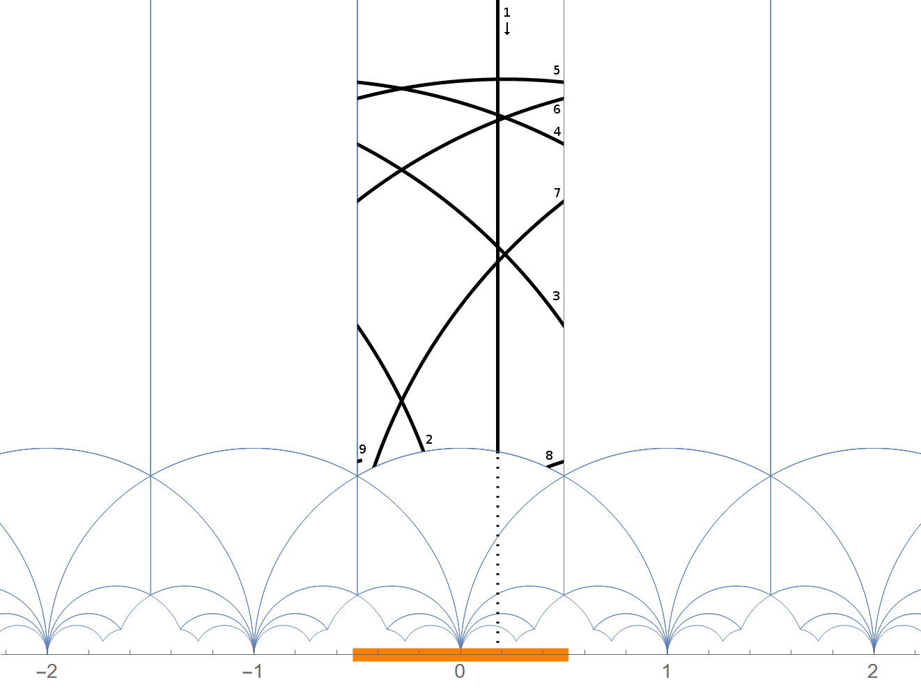
Consider now the subsegment $\gamma^{\prime}$ of $\gamma$ strictly between the intersection with $\mathbb{S}$ and before the intersection with $M_{1}\mathbb{S}$. The intersection of $\gamma$ with $M_{1}\mathbb{S}$ can be used to recover the first CF digit of $\gamma_{+}$, since we have that $M_{1}^{-1}(z)=-1/z+a_{1}$. However, intersections of $\gamma^{\prime}$ with other $\mathcal{M}$-translates of $\mathbb{S}$ do not correspond to digits of $\gamma_{+}$. We wish to find a subset of $\mathbb{S}$ for $\gamma$ to intersect with that does not detect these ‘‘spurious’’ intersections of $\gamma^{\prime}$ seen in Figure 4a, but does continue to detect (most of) the crossings of $\gamma$ with $M_{i}\mathbb{S}$. In this way intersections of $\gamma$ with $\mathcal{M}\mathbb{S}$ correspond strongly to iterations of the shift map $T^{i}$ on $\gamma_{+}$, and so the behavior of geodesic flow will strongly correlate to the behavior of the shift map $T$. We will do this in the unit tangent bundle of $\mathbb{H}^{2}_{\mathbb{R}}$, by restricting the allowed unit vectors over $\mathbb{S}$. The process is summarized in Figure 4.

We first quickly prove that $M_{1}^{-1}\gamma$ in fact crosses $\mathbb{S}$. Indeed, we have that $M_{1}^{-1}\gamma_{+}$ is inside $\mathbb{S}$, while $\left|a_{i}\right|\geq 2$, so that $M_{1}^{-1}(\gamma_{-})=M_{1}^{-1}(\infty)=-a_{i}$ is outside of $\mathbb{S}$. While this bound appears to deteriorate to $\left|M_{i}^{-1}\gamma_{-}\right|\geq 1$ with additional iterations, by looking at the permissible digits one shows that $\left|M_{i}^{-1}\gamma_{-}\right|$ is bounded below by the golden ratio $\phi$. See Remark 1.5 for the more general approach to this step.

In Figure 4a, we see that $\gamma^{\prime}$ has (at least) two intersections occur that we do not want to code: the intersection with the sphere centered at the point $(1,0)$, and the intersection with the vertical line $x=1.5$. The first of these is avoided simply by restricting to the vectors in $T^{1}\mathbb{S}$ that point towards $K=[-1/2,1/2)$ (i.e., whose corresponding geodesics terminate in $K$). By completeness, any (non-identity) $\mathcal{Z}$-translate of these vectors must land outside of $K$. In particular, the corresponding vectors on the sphere centered at $(1,0)$ point to the interval $[1/2,3/2)$, whereas we know that $M_{1}^{-1}\gamma_{+}\in K$. Thus this intersection is avoided.

The second spurious intersection in our example requires more work, and we rule it out by making two observations about $M_{1}^{-1}\gamma^{\prime}$ that are predicated on the use of horoheight and horoballs (shown in green in Figure 4, cf. Ford circles). We may measure horoheight either from $\infty$, in which case horoheight is simply the $y$ coordinate and a horoball is a set of the form $\{(x,y):y>y_{0}\}$, or from a (rational) point on the $x$-axis, in which case horoheight can be thought of as depth into the corresponding cusp, and horoballs appear as Euclidean disks tangent to the $x$-axis. For our first observation, the fact that $\left|M^{-1}_{1}\gamma_{+}\right|\leq 1/2$ and $\left|M^{-1}_{1}\gamma_{-}\right|\geq\phi$ implies that the intersection of $M^{-1}_{1}\gamma^{\prime}$ with $\mathbb{S}$ occurs away from the $x$-axis, in the smaller ‘‘wall’’ region (see Figure 4b)

and that the intersection with $M^{-1}_{1}\mathbb{S}$ is likewise bounded away from the $x$-axis. That is, $M_{1}^{-1}\gamma^{\prime}$ is contained in a horoball $\mathcal{B}=\{y>\epsilon\}$ for some $\epsilon>0$. For our second observation, consider a mapping $M\in\mathcal{M}$ that sends the line $x=1.5$ to $\mathbb{S}$. Normalizing $M_{1}^{-1}\gamma^{\prime}$ further by $M$, we see (Figure 4c) that $MM_{1}^{-1}\gamma^{\prime}\subset M\mathcal{B}$ is now contained in one of the horoballs based at a finite rational point. In particular, this provides (see Corollary 5.6) an upper bound $c=\left(\frac{3}{2}(5\sqrt{5}-11)\right)^{-1/2}\approx 1.923$ on how far $MM_{1}^{-1}\gamma^{\prime}$ travels away from the $x$-axis. We can reject the intersection of $MM_{1}^{-1}\gamma^{\prime}$ with $\mathbb{S}$ (and thus the intersection of $M_{1}^{-1}\gamma^{\prime}$ with the line $x=1.5$) by restricting to the vectors in $T^{1}\mathbb{W}$ that are returning from a cusp excursion towards $\infty$ of depth at least $c$. We will denote by $\mathcal{C}_{\mathbb{W}}$ the set of such vectors that also point towards $K$. This is our desired refinement of $\mathbb{S}$ (Figure 4d).

Our choice of $\mathcal{C}_{\mathbb{W}}$ by construction avoids all spurious intersections, but may also inadvertently ignore some intersections corresponding to small digits or even entire geodesics. We say that a geodesic $\gamma$ is markable if it intersects $\mathcal{M}$-translates of $\mathcal{C}_{\mathbb{W}}$ infinitely often in both the past and future, and it is easy to see that almost every geodesic is markable, see Corollary 6.6. The Markable Geodesic Theorem 5.1 records the desired link between the CF digits of a markable geodesic $\gamma$ and its intersections with $\mathcal{M}$-translates of $\mathcal{C}_{\mathbb{W}}$: intersections occur only with walls of the form $M_{i}\mathcal{C}_{\mathbb{W}}$, the intersections occur in the desired order, and no other intersections occur.

With the section $\mathcal{C}_{\mathbb{W}}$ in hand, we return to the question of ergodicity. We begin by working through a number of closely related functions acting on different spaces, pulling ergodicity from one function to the next. The ergodicity of geodesic flow on the modular surface $\mathcal{M}\backslash\mathbb{H}^{2}_{\mathbb{R}}$ implies the ergodicity of the first return map to the projection of $\mathcal{C}_{\mathbb{W}}$ onto the modular surface. We can then lift this first return map back to $\mathbb{H}^{2}_{\mathbb{R}}$ to obtain an isomorphic and thus equally ergodic map $\psi:\mathcal{C}_{\mathbb{W}}\to\mathcal{C}_{\mathbb{W}}$ (Proposition 6.9). We then conjugate this system with the projection $\pi$ from the unit tangent bundle of $\mathbb{H}^{2}_{\mathbb{R}}$ to $\hat{\mathbb{R}}\times\hat{\mathbb{R}}$ that takes any geodesic $\gamma$ to its forward and backward endpoints $(\gamma_{+},\gamma_{-})$, obtaining an ergodic mapping $\Psi=\pi\circ\psi\circ\pi^{-1}$ on $\pi(\mathcal{C}_{\mathbb{W}})$. This map acts by taking a point $(\gamma_{+},\gamma_{-})$ to $(M_{i}^{-1}\gamma_{+},M_{i}^{-1}\gamma_{-})$ for some $i$. Thus, in the first coordinate, $\Psi$ acts by $T^{i}$, where $i$ may depend on the value of $\gamma_{+}$, i.e., this is a jump transformation associated to $T$.

Although we could conclude this jump transformation is ergodic, the ergodicity of a jump transformation does not imply the ergodicity of the original map in general. So to recover the ergodicity of $T$, we step back to $\hat{\mathbb{R}}\times\hat{\mathbb{R}}$. Namely, we consider a natural-extension-like function $\hat{T}$ on $K\times\hat{\mathbb{R}}$ such that the action of $\hat{T}$ on the first coordinate is simply $T$. We show that the action of $\hat{T}$ on $\overline{K}=\bigcup_{i=0}^{\infty}\hat{T}^{i}\pi(\mathcal{C}_{\mathbb{W}})$ is well-behaved (Lemma 6.10) and that, in fact, $\Psi$ is simply the map induced by restricting $\hat{T}$ to $\pi(\mathcal{C}_{\mathbb{W}})$ (Lemma 6.11). Induced maps have far greater structure than jump transformations and so we are able to conclude the ergodicity of $\hat{T}$ on $\overline{K}$ from the ergodicity of $\Psi$ (Lemma 6.12) and from there conclude the ergodicity of $T$ by restricting to the first coordinate.

Iwasawa CFs are the most general setting for our methods, which rely heavily on the fact that Iwasawa inversion spaces are boundaries of rank one symmetric spaces of non-compact type. Indeed, Iwasawa inversion spaces are precisely the spaces with this property, with the exclusion, due to the break down of vector-space-based techniques, of the exceptional $\mathbb{X}^{1}_{\mathbb{O}}$ that can be defined over the non-associative octonions. Our notion of Iwasawa inversion space differs slightly from the notion of Iwasawa groups of [9], which excludes $\mathbb{X}^{n}_{\mathbb{R}}$ and allows $\mathbb{X}^{1}_{\mathbb{O}}$.

We remark further that boundaries of rank one symmetric spaces of non-compact type are arguably the most general setting for geometric CFs and Diophantine theory: they are characterized [37, 12] as homogeneous geodesic locally compact spaces admitting both a dilation (a notion of fraction) and a well-behaved inversion. (The Cygan metric we work with is not itself geodesic, but gives rise to a geodesic path metric.)

The present work suggests the following further directions of study:

Following this introduction, in §2 we provide the general theory and definitions for Iwasawa inversion spaces. In §3 we define Iwasawa CFs, give further examples (including Table 1) and study conditions that guarantee discreteness, properness, and completeness. In §4, we quickly prove the convergence of Iwasawa CFs. In §5, we will build up the theory surrounding markable geodesics, culminating in the Markable Geodesic Theorem. In §6, we use the Markable Geodesic Theorem to prove the ergodicity of the CF shift map for an Iwasawa CF expansion and, in applications of this result, prove Theorems 1.3 and 1.4.

A.L. was supported by University of Michigan NSF RTG grant 1045119. This article was written during visits by the authors to University of Texas at Tyler, George Mason University, University of Michigan, and the Ohio State University. The authors thank these institutions for their hospitality, and Simons Travel Grant and GEAR Grant NSF DMS 11-07452 for the travel funding. The authors would also like to thank Jayadev Athreya and Ralf Spatzier for their helpful comments, and the anonymous referee for the extensive suggestions that improved the exposition of this paper.

Abstractly, an Iwasawa inversion space $\mathbb{X}$ is an Iwasawa $N$-group associated by the Iwasawa (KAN) decomposition to a non-exceptional rank one semi-simple Lie group $G$ and the parabolic boundary at infinity of the rank one symmetric space $G/K$. We now recall the explicit construction and Euclidean-like structure of these spaces. Most of the contents of this section can be found in [9, 20, 51].

Fix an associative division algebra $k$ over the reals --- the real, complex, or quaternionic numbers⁷⁷ 7 When working over quaternions, we will use the convention $\frac{p}{q}:=pq^{-1}$. — and an integer $n\geq 1$. (It appears that one could also consider the exceptional case of octonions, but we will not do so here.) Recall that $k$ has a real part $\text{Re}(k)$ isomorphic to $\mathbb{R}$ and a complementary imaginary part $\text{Im}(k)$ satisfying $\dim_{\mathbb{R}}(\text{Im}(k))=\dim_{\mathbb{R}}(k)-1$. We denote the standard norm of an element of $k$ or $k^{n}$ by $\left\|\cdot\right\|$, and refer to $\left\|\cdot\right\|$-preserving $k$-linear automorphisms of $k^{n}$ as unitary transformations.

Over the reals, $\mathbb{X}^{n}_{\mathbb{R}}$ reduces to $\mathbb{R}^{n}$ with $*$ acting by the usual vector addition. For $k\neq\mathbb{R}$, $\mathbb{X}^{n}_{k}$ is a step-2 nilpotent group (one uses $*$ to emphasize the non-commutativity), with identity $(0,0)$, and the inverse of a group element $(z,t)$ given by $(-z,-t)$.

One gives $\mathbb{X}$ a gauge $\left|\cdot\right|$ and Cygan metric $d$ (also known in different contexts as the Korányi metric or gauge metric) by defining

The Cygan metric is largely analogous to the Euclidean metric, insofar as its automorphisms include analogs of translations (left multiplication by an element of $\mathbb{X}$ is an isometric isomorphism); dilations (for each $r>0$, the mapping $\delta_{r}(z,t)=(rz,r^{2}t)$ is a group isomorphism that rescales the metric by factor $r$); and rotations (unitary automorphisms of $k^{n}$ extend to isometric group isomorphisms of $\mathbb{X}$).

On the other hand, the metric is fractal for $k\neq\mathbb{R}$: it is not a path metric (cf. the closely associated Carnot-Carathéodory path metric) and gives $\mathbb{X}$ Hausdorff dimension $n\dim_{\mathbb{R}}(k)+2(\dim_{\mathbb{R}}(k)-1)$ which is not equal to its topological dimension $(n+1)\dim_{\mathbb{R}}(k)-1$. The latter is due to the fact that large metric balls are stretched by $\delta_{r}$ along the $t$ direction, while small ones are flattened out along the $z$ direction.

The Korányi inversion $\iota_{-}:\mathbb{X}\setminus\{0\}\rightarrow\mathbb{X}\setminus\{0\}$ is defined by

The Korányi inversion is a natural generalization of the mapping $x\mapsto-1/x$, and in particular satisfies the following pair of identities for $h,h^{\prime}\in\mathbb{X}\setminus\{0\}$, [12]:

In particular, $\iota_{-}$ sends each sphere $S(0,r)$ to the sphere $S(0,1/r)$, and preserves the unit sphere. We prove the identities in a broader context in Theorem 2.11.

More generally, $\mathbb{X}$ admits inversions of the form

where $A$ is a unitary transformation of $k^{n}$. We show in Lemma 2.10 that all inversions satisfy generalizations of Equations 2.1.

Fix an Iwasawa inversion space $\mathbb{X}=\mathbb{X}^{n}_{k}$. We extend the structure and Cygan metric of $\mathbb{X}$ to $k^{n+1}$ as follows, motivated by Parker [51]:

Consider the Hermitian form $\langle\cdot,\cdot\rangle_{J}$ of signature $(n+1,1)$ defined on $k^{n+2}$ by

and let $\mathcal{S}=\{(1:a:b)\;:\;\left\|a\right\|<2\text{Re}(b)\}\subset\mathbb{P}(k^{n+2})$ be the Siegel region. One can show that $\Phi$ induces a bijection between $\mathbb{H}$ and $\mathcal{S}$, and furthermore $\mathcal{S}$ is the projectivization of the negative cone of $J$. This induces an action of the projective unitary group $G=\mathbb{P}U(J)$ on $\mathbb{H}$, cf. §4.

For $\mathbb{H}=\mathbb{H}^{2}_{\mathbb{R}}$, $d_{\mathbb{H}}$ is agrees with the familiar metric $\frac{1}{y}ds$ if one takes $x=z$ and $y=w^{2}$. One has $\Phi(\mathbb{H})=\{(1:a:b)\;:\;2b>a^{2}\}\subset\mathbb{RP}^{2}$, and a projective change of coordinates recovers the Klein disk model of $\mathbb{H}^{2}_{\mathbb{R}}$ with its $SO(2,1)$-invariant metric.

In general, the Siegel region is projectively equivalent to a unit ball in projective space $\mathbb{P}(k^{n+2})$. The mapping $\Phi|_{\mathbb{X}}:\partial\mathbb{H}\rightarrow\partial\Phi(\mathbb{H})$ omits a single point, which we identify with the point $\infty$ in the one-point compactification of $k^{n+1}$ (and its subsets $\mathbb{X}$ and $\overline{\mathbb{H}}$).

Returning to the Cygan metric, we record two connections to the projective embedding:

With the above machinery, we can provide a simple description of the Korányi inversion, extended to $\overline{\mathbb{H}}$, and prove the inversion identities (2.1).

References

- [1] Roy L. Adler and Leopold Flatto, The backward continued fraction map and geodesic flow, Ergodic Theory Dynam. Systems 4 (1984), no. 4, 487–492. MR 779707
- [2] Pierre Arnoux and Thomas A. Schmidt, Cross sections for geodesic flows and -continued fractions, Nonlinearity 26 (2013), no. 3, 711–726. MR 3018939
- [3] Emil Artin, Ein mechanisches system mit quasiergodischen bahnen, Abh. Math. Sem. Univ. Hamburg 3 (1924), no. 1, 170–175. MR 3069425
- [4] M. Bauer and A. Lopes, A billiard in the hyperbolic plane with decay of correlation of type , Discrete Contin. Dynam. Systems 3 (1997), no. 1, 107–116. MR 1422542
- [5] Florin P Boca and Claire Merriman, Coding of geodesics on some modular surfaces and applications to odd and even continued fractions, Indagationes Mathematicae 29 (2018), no. 5, 1214–1234.
- [6] Robert Burton, Cornelis Kraaikamp, and Thomas Schmidt, Natural extensions for the Rosen fractions, Transactions of the American Mathematical Society 352 (2000), no. 3, 1277–1298.
- [7] Kariane Calta and Thomas A. Schmidt, Continued fractions for a class of triangle groups, J. Aust. Math. Soc. 93 (2012), no. 1-2, 21–42. MR 3061992
- [8] Wensheng Cao and John R. Parker, Shimizu’s lemma for quaternionic hyperbolic space, Comput. Methods Funct. Theory 18 (2018), no. 1, 159–191. MR 3764717
- [9] Vasilis Chousionis, Jeremy Tyson, and Mariusz Urbański, Conformal graph directed Markov systems on Carnot groups, Mem. Amer. Math. Soc. 266 (2020), no. 1291, viii+155. MR 4126256
- [10] Bastiaan Cijsouw, Complex continued fraction algorithms, Master’s thesis, Radboud University, 2015.
- [11] John H. Conway and Derek A. Smith, On quaternions and octonions: their geometry, arithmetic, and symmetry, A K Peters, Ltd., Natick, MA, 2003. MR 1957212
- [12] Michael Cowling, Anthony H Dooley, Adam Korányi, and Fulvio Ricci, H-type groups and Iwasawa decompositions, Advances in Mathematics 87 (1991), no. 1, 1 – 41.
- [13] Karma Dajani, Doug Hensley, Cor Kraaikamp, and Valentina Masarotto, Arithmetic and ergodic properties of ‘flipped’ continued fraction algorithms, Acta Arithmetica 153 (2012), no. 1, 51–79.
- [14] Karma Dajani and Cor Kraaikamp, Ergodic theory of numbers, vol. 29, American Mathematical Soc., 2002.
- [15] Karma Dajani, Cor Kraaikamp, and Wolfgang Steiner, Metrical theory for -Rosen fractions, J. Eur. Math. Soc. (JEMS) 11 (2009), no. 6, 1259–1283. MR 2557135
- [16] Karma Dajani, Cor Kraaikamp, and Niels van der Wekken, Ergodicity of -continued fraction expansions, J. Number Theory 133 (2013), no. 9, 3183–3204. MR 3057071
- [17] S. G. Dani, Continued fraction expansions for complex numbers—a general approach, Acta Arith. 171 (2015), no. 4, 355–369. MR 3430769
- [18] Hiromi Ei, Shunji Ito, Hitoshi Nakada, and Rie Natsui, On the construction of the natural extension of the Hurwitz complex continued fraction map, Monatshefte für Mathematik 188 (2019), no. 1, 37–86.
- [19] Manfred Einsiedler and Thomas Ward, Ergodic theory with a view towards number theory, Graduate Texts in Mathematics, vol. 259, Springer-Verlag London, Ltd., London, 2011. MR 2723325
- [20] William M. Goldman, Complex hyperbolic geometry, Oxford Mathematical Monographs, The Clarendon Press, Oxford University Press, New York, 1999, Oxford Science Publications. MR 1695450
- [21] Karlheinz Gröchenig and Andrew Haas, Backward continued fractions, Hecke groups and invariant measures for transformations of the interval, Ergodic Theory Dynam. Systems 16 (1996), no. 6, 1241–1274. MR 1424398
- [22] William R. Hamilton, On continued fractions in quaternions, Phil. Mag., iii (1852), 371–373; iv (1852), 303; v (1853), 117–118, 236–238, 321–326.
- [23] by same author, On the connexion of quaternions with continued fractions and quadratic equations, Proc. Royal Irish Acad. 5 (1853), 219–221, 299–301.
- [24] Grant Paul Hayward, The action of the Picard group on hyperbolic 3-space and complex continued fractions, Ph.D. thesis, University of the Witwatersrand, Faculty of Science, School of Mathematics, 2014.
- [25] Gustav A Hedlund, A metrically transitive group defined by the modular groups, American Journal of Mathematics 57 (1935), no. 3, 668–678.
- [26] Doug Hensley, Continued fractions, World Scientific Publishing Co. Pte. Ltd., Hackensack, NJ, 2006. MR 2351741
- [27] Sa’ar Hersonsky and Frédéric Paulin, Diophantine approximation for negatively curved manifolds, Mathematische Zeitschrift 241 (2002), no. 1, 181–226.
- [28] Ghaith Hiary and Joseph Vandehey, Calculations of the invariant measure for Hurwitz continued fractions, Experimental Mathematics (2019), 1–13.
- [29] Robert Hines, Badly approximable numbers over imaginary quadratic fields, Acta Arith. 190 (2019), no. 2, 101–125. MR 3984261
- [30] Adolf Hurwitz, Über die Entwicklung complexer Grössen in Kettenbrüche, Acta Math. 11 (1887), no. 1-4, 187–200. MR 1554754
- [31] by same author, Über eine besondere Art der Kettenbruch-Entwicklung reeller Grössen, Acta Math. 12 (1889), no. 1, 367–405. MR 1554778
- [32] Shunji Ito and Michiko Yuri, Number theoretical transformations with finite range structure and their ergodic properties, Tokyo J. Math 10 (1987), 1–32.
- [33] Svetlana Katok and Ilie Ugarcovici, Arithmetic coding of geodesics on the modular surface via continued fractions, European women in mathematics—Marseille 2003, CWI Tract, vol. 135, Centrum Wisk. Inform., Amsterdam, 2005, pp. 59–77. MR 2223106
- [34] by same author, Symbolic dynamics for the modular surface and beyond, Bull. Amer. Math. Soc. (N.S.) 44 (2007), no. 1, 87–132. MR 2265011
- [35] by same author, Applications of -continued fraction transformations, Ergodic Theory Dynam. Systems 32 (2012), no. 2, 755–777. MR 2901369
- [36] Richard B. Lakein, Continued fractions and equivalent complex numbers, Proc. Amer. Math. Soc. 42 (1974), 641–642. MR 0382179
- [37] Enrico Le Donne, A metric characterization of Carnot groups, Proc. Amer. Math. Soc. 143 (2015), no. 2, 845–849. MR 3283670
- [38] Anton Lukyanenko and Joseph Vandehey, Continued fractions on the Heisenberg group, Acta Arith. 167 (2015), no. 1, 19–42. MR 3310489
- [39] by same author, Intrinsic Diophantine approximation in Carnot groups and in the Siegel model of the Heisenberg group, Monatsh. Math. 192 (2020), no. 3, 651–676. MR 4109520
- [40] S. Marmi, P. Moussa, and J.-C. Yoccoz, The Brjuno functions and their regularity properties, Comm. Math. Phys. 186 (1997), no. 2, 265–293. MR 1462766
- [41] Valentina Masarotto, Metric and arithmetic properties of a new class of continued fraction expansions, Ph.D. thesis, Master Thesis, Universita di Padova and Leiden University, 2009.
- [42] F. I. Mautner, Geodesic flows on symmetric Riemann spaces, Ann. of Math. (2) 65 (1957), 416–431. MR 0084823
- [43] Dieter Mayer and Fredrik Strömberg, Symbolic dynamics for the geodesic flow on Hecke surfaces, J. Mod. Dyn. 2 (2008), no. 4, 581–627. MR 2449139
- [44] Carminda Margaretha Mennen, The algebra and geometry of continued fractions with integer quaternion coefficients, Ph.D. thesis, University of the Witwatersrand, 2015.
- [45] Hitoshi Nakada, On the Kuzmin’s theorem for the complex continued fractions, Keio Engrg. Rep. 29 (1976), no. 9, 93–108. MR 463401
- [46] by same author, Metrical theory for a class of continued fraction transformations and their natural extensions, Tokyo J. Math. 4 (1981), no. 2, 399–426. MR 646050
- [47] by same author, On ergodic theory of A. Schmidt’s complex continued fractions over Gaussian field, Monatsh. Math. 105 (1988), no. 2, 131–150. MR 930432
- [48] Hitoshi Nakada and Rie Natsui, On the equivalence relations of -continued fractions, Indagationes Mathematicae 25 (2014), no. 4, 800–815.
- [49] Hitoshi Nakada and Wolfgang Steiner, On the ergodic theory of Tanaka–Ito type -continued fractions, Tokyo Journal of Mathematics 1 (2021), no. 1, 1–15.
- [50] Giovanni Panti, Slow continued fractions, transducers, and the Serret theorem, Journal of Number Theory 185 (2018), 121–143.
- [51] John R. Parker, Shimizu’s lemma for complex hyperbolic space, Internat. J. Math. 3 (1992), no. 2, 291–308. MR 1146815
- [52] Mark Pollicott, The Picard group, closed geodesics and zeta functions, Trans. Amer. Math. Soc. 344 (1994), no. 2, 857–872. MR 1240946
- [53] Asmus L Schmidt, Diophantine approximation of complex numbers, Acta mathematica 134 (1975), no. 1, 1–85.
- [54] F Schweiger and M Waterman, Some remarks on Kuzmin’s theorem for F-expansions, Journal of Number Theory 5 (1973), no. 2, 123–131.
- [55] Fritz Schweiger, Ergodic theory of fibred systems and metric number theory, Oxford Science Publications, The Clarendon Press, Oxford University Press, New York, 1995. MR 1419320
- [56] Fritz Schweiger et al., Multidimensional continued fractions, Oxford University Press on Demand, 2000.
- [57] Caroline Series, The modular surface and continued fractions, J. London Math. Soc. (2) 31 (1985), no. 1, 69–80. MR 810563
- [58] Iekata Shiokawa, Ryuji Kaneiwa, and Jun-ichi Tamura, A proof of Perron’s theorem on Diophantine approximation of complex numbers, Keio Engrg. Rep. 28 (1975), no. 12, 131–147. MR 0429773
- [59] Shigeru Tanaka, A complex continued fraction transformation and its ergodic properties, Tokyo J. Math. 8 (1985), no. 1, 191–214. MR 800085
- [60] Shigeru Tanaka and Shunji Ito, On a family of continued-fraction transformations and their ergodic properties, Tokyo J. Math. 4 (1981), no. 1, 153–175. MR 625125
- [61] William Thurston, Geometry and topology of three-manifolds, 1980.
- [62] Joseph Vandehey, Lagrange’s theorem for continued fractions on the Heisenberg group, Bull. Lond. Math. Soc. 47 (2015), no. 5, 866–882. MR 3403968
- [63] by same author, Non-trivial matrix actions preserve normality for continued fractions, Compos. Math. 153 (2017), no. 2, 274–293. MR 3705225
- [64] Robert J. Zimmer, Ergodic theory and semisimple groups, Monographs in Mathematics, vol. 81, Birkhäuser Verlag, Basel, 1984. MR 776417
- [65] Иванъ Владиславовичъ Слешинскй, Дополнение къ заметке о сходимости непрерывныхъ дробей, Математический сборник 14 (1889), no. 3, 436–438.