Memory efficient distributed sliding super point cardinality estimation by GPU

Suppose there are two networks $ANet$ and $BNet$. These two networks are contacting with each other through a set of edge routers $ER$. $ANet$ might be a city-wide network or even a country-wide network. And $BNet$ might be another city-wide network or the Internet. All traffic between $ANet$ and $BNet$ could be observed from $ER$. Split this traffic by successive time slices as shown in figure 1.

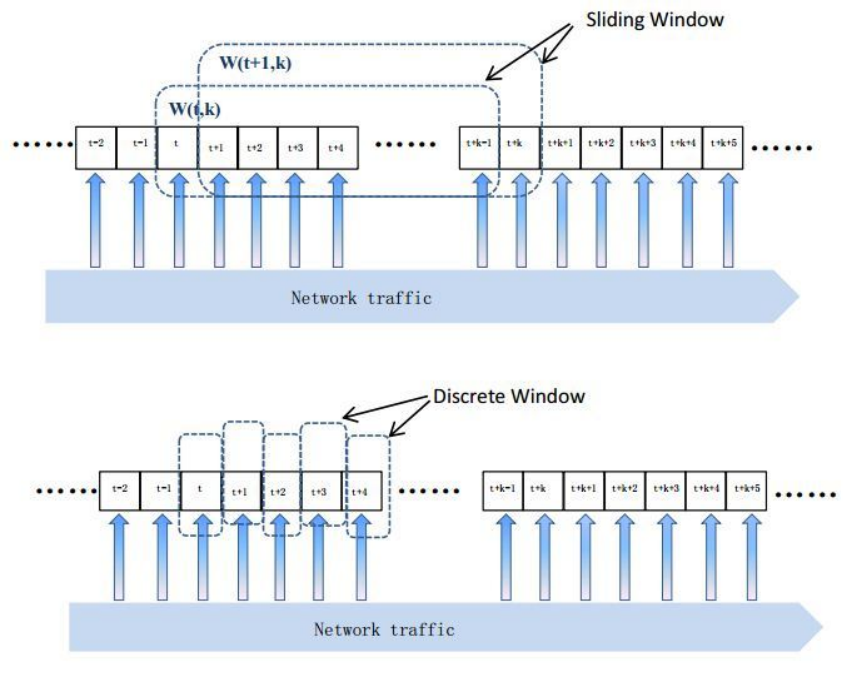
These time slices have the same duration. The length of a time slice could be 1 second, 1 minute or any period in different situations. Every time slice is identified by a number. A sliding time window $W(t,k)$ contains $k$ successive slices starting from the $t$ time slice as shown in the top part of figure 1. Sliding time window will move forward one slice once a time. So two adjacent sliding time windows contain $k-1$ same slices. When $k$ is set to 1, there is no duplicate time period between two adjacent windows, which is the case of discrete time window in the bottom part of figure 1.

Let $ANet$ be the network from which we want to detect super points. A host’s packets stream in a sliding time window is defined as below.

$aip$’s opposite hosts stream $ST(aip,t,k)$ could be derived from $Pkt(aip,t,k)$ by extracting the other IP address except $aip$. A IP address $bip$ may appear several times in $ST(aip,t,k)$ because $aip$ can send several packets to $bip$ or receive many packets from $bip$. Hosts in $ST(aip,t,k)$ make up of opposite hosts set of $aip$, written as $OH(aip,t,k)$. The number of element in $OH(aip,t,k)$, denoted as $|OH(aip,t,k)$, is no bigger than that of $ST(aip,t,k)$. $|OH(aip,t,k)|$ is the cardinality of $aip$ in sliding time window $W(t,k)$. Sliding super point is defined according to host’s cardinality.

When $k=1$, sliding super point could be called as super point. Threshold $\theta$ is defined by users for different applications. It could be selected according to the average cardinality of all host in the past or the normal cardinality of a server. How to get $|OH(aip,t,k)|$ from $ST(aip,t,k)$ is a hard task. Because packets pass through $ER$ with high speed and every packet could only be scanned a time in the stream. How to process every coming packet and give an accurate estimation of $|OH(aip,t,k)|$ at the end of the last time slice of $W(t,k)$ is the key step in the whole algorithm.

The key step of sliding super point detecting is to determine if a host is a super point in a sliding time window. Because discrete time window is a special case of sliding time window and working under discrete time window is much simpler than that under sliding time window, we firstly introduce how to judge super point under discrete time window and then give its sliding time window version.

For a host $aip$, the task of judging super point under discrete time window is to determine if $|OH(aip,t,1)|\geq\theta$ by scanning every host in $ST(aip,t,1)$ once. Rough estimator $RE$ proposed in this paper is a memory efficient algorithm which can tell if a host is a super point in a time period with only 8 bits. These 8 bits are initialized to zero at the begin of a time period. $RE$ samples and records hosts in $ST(aip,t,1)$ by the least significant bits of their hashed values. Least significant bit of an integer is defined in the below.

For example, $LSB(3)=0$, $LSB(40)=3$. The binary formatters of 3 and 40 are "11" and "101000". The first bit of $BIN(3)$ is ‘1’, so $LSB(3)$ equals to 0. While $BIN(40)$ meets its first ‘1’ until the fourth bit, so its $LSB$ is 3. For every host $bip$ in $OH(aip,t,1)$, RE hashes it to a random value between 0 and $2^{32}-1$ by a hash function $H_{1}$ (20). If $LSB(H_{1}(bip))$ is smaller than an integer $\tau$, this IP will not be recorded by $RE$ where $\tau$ is derived from $\theta$ by equation 1.

When $LSB(H_{1}(bip))\geq\tau$, a bit selected by $H_{2}(bip)$ will be set where $H_{2}$ is another hash function mapping $bip$ to a value between 0 and $\eta-1$.

$RE$ deals with every host in $ST(aip,t,1)$ in this way. At the end of slice $t$, if the number of ‘1’ bits is no smaller than $\rho*\eta$, $|OH(aip,t,1)|$ is judged as bigger than $\theta$ by $RE$, where $\rho=0.99*(1-e^{-1/3})$. $\rho$ is acquired from (21).

$RE$ has a high probability to report a super point.

Suppose there are $\alpha$ hosts in $OH(aip,t,1)$ updating $RE$. The probability that there are $\eta_{1}$ bits are set to 1 is :

Every host in $OH(aip,t,1)$ has probability $\frac{1}{2^{\tau}}$ to update $RE$. So the probability that there are $\alpha$ hosts in $OH(aip,t,1)$ updating $RE$ is:

Combine equation 2 and 3, we will get the probability that there are $\eta_{1}$ ‘1’ bits in $RE$ after scanning $ST(aip,t,1)$ as shown in equation 4.

.

The probability that there are more than ${\eta}_{1}$ ‘1’ bits in $RE$ after scanning $ST(aip,t,1)$ could be derived from 4 as shown in equation 5.

Equation 5 proofs that $RE$ has a high probability to detect super point in discrete time window. There is only one time slice in $W(t,1)$. So one bit is enough to represent if a host appears in this slice. But when $k>1$, a single bit can’t know if some hosts still appear in $W(t+1,k)$ when the window sliding from $W(t,k)$.

Unlike discrete version using $\eta$ bits, $RE$ sliding version $SRE$ uses $\eta$ short integers, where each short integer is unsigned short integer with 16 bits, to record host’s cardinality. $SRE$ has five operations: initialization, hosts scanning, super point detection, slice updating, $SRE$s merging.

Before $SRE$ launching, every short integer will be initialized to the biggest value 65535. Like $RE$, $SRE$ scans every host in a time slice $t+k-1$ by hashing the host, comparing the LSB of hashed value with $\tau$. When the hashed value is no smaller than $\tau$, an short integer will be selected and set to 0, unlike $RE$ which sets a bit to 1. Let $SRE[i]$ point to the $i$th short integer in $SRE$. The weight of $RE$ is the number of 1 bits in it. But the weight of $SRE$ is the number of integer whose value is smaller than $k$, denoted as $|SRE|^{k}$. $SRE$ will check $aip$ at the end of time slice $t+k-1$. It judges if $aip$ is super point by comparing its weight $|SRE|^{k}$ with $\eta*\rho$ like $RE$. After checking $aip$, the window will slide to $W(t+1,k)$. $SRE$ will not initialize its short integers at the beginning of a new time slice. But every short integer will increment 1 before scanning new hosts in this time slice. A short integer in $SRE$ records the distance between the nearest time slice when it is set and the scanning time slice. So when the window moves forward, the distance will grow too. If a short integer is mapped by some host in the time slice, the distance is 0. When merging two $SRE$s together, short integers in the new $SRE$ will be selected from the biggest ones. Algorithm 1 and 2 describe the hosts scanning and $SRE$ merging process.

There is no accessing conflict in $SRE$ which means $SRE$ could deal with several hosts parallel to speed up the process. $SRE$ can determine if a host is super point in a window. But there are millions of hosts in $ANet$ for a high speed network. It’s too expensive and slow to allocate a $SRE$ for every host in $ANet$. A smart structure based on $SRE$ is devised to solve this problem. The new algorithm uses a fixed number of $SRE$s to record hosts and restore sliding super points at the end of a time slice as shown in the next part.

Many hosts in $ANet$ have a smaller cardinality. Allocating a $SRE$ for every host will waste lots of memory and slow down hosts scanning speed. Based on $SRE$, a smart structure, called as reversible sliding rough estimator array RSRA, is proposed. RSRA contains $2^{q}$ columns and r rows of sliding rough estimators as shown in figure 2. Let RSRA[i,j] point to the $SRE$ in the $i$th row, $j$th column. This structure is reversible because sliding super point could be reconstructed from it without any other data. This reversible ability comes from a novel hash functions group, reversible hash functions group RHFG.

RHFG is an array of r hash functions, each of which hashes an IP address to a value between 0 and $2^{q}-1$. Let RHFG[i] represent the $i$th hash function. RHFG[0] is a random hash function (22) which maps a IP address to an integer between 0 and $2^{q}-1$, $0\leq RHFG[0](aip)\leq 2^{q}-1$ where $aip\in ANet$. The rest $r-1$ hash functions are derived from $RHFG[0]$ according the following equation.

In equation 6, $1\leq i\leq r-1$, $aip\in ANet$. $\delta$ is an positive integer that smaller than q and $(r-2)*\delta+q\geq 32$. “XOR" is the bit wise exclusive or operation. "$>>$" is the bit wise right shift operation. According to the property of “XOR", we can recover $(aip>>(i*\delta))mod(2^{q})$ by equation 7.

$(aip>>(i*\delta))mod(2^{q})$ is q successive bits of $aip$ starting from $i*\delta$, written as $B(i)$. Because $(r-2)*\delta+q\geq 32$, every bit in $aip$ will appear in some $B(i)$ where $1\leq i\leq r-1$. For a host $aip\in ANet$, let RHFG(aip) represent the array of r hashed values where $RHFG(aip)=\{RHFG[0](aip),RHFG[1](aip)$ $,\cdots,RHFG[r-1](aip)\}$. $aip$ could be regained from $RHFG(aip)$ by extracting bits from $B(i)$.

$RHFG$ has high randomness and reversible ability. It is used to select $r$ sliding rough estimators from each row of RSRA for every host in $ANet$. For a host $aip$ in $ANet$, its r sliding rough estimators are denoted as $RSRA(aip)=\{RSRA[0,RHFG[0](aip)]$ $,RSRA[1,RHFG[1](aip)]$ $,\cdots,$ $RSRA[r-1,RHFG[r-1]$ $(aip)]\}$. A IP pair is a set of two IP addresses extracting from a packet where one address is in $ANet$ and the other is in $BNet$. When a IP pair comes, these r sliding rough estimators will be updated at the same time as shown in algorithm 3.

Algorithm 3 describes how to update RSRA for a IP pair. But there are millions of IP pairs every second for example in a 40 Gb/s network. Dealing with these IP pairs one by one will consume much time for a single thread. In algorithm 3 only line 14 update memory while others are computing operations such as getting sliding estimator index in RSRA, calculating which distance recorder to be set. A distance recorder could be set to zero multi times which makes sure that there is no need to synchronize among memory access and several IP pairs could update RSRA at the same time.

Nowadays CPU contains several cores, from 2 to 22 or more such as Intel E5-2699v4. When exploiting all cores of CPU to scan IP pairs parallel, the processing speed will be raised. But the memory bandwidth of CPU will limit the increment. What’s more, the price of CPU grows rapidly with the number of cores because the single core of CPU is so powerful, high frequency and complex control ability, that it occupies much space on chip.

Unlike CUP’s core, each core of GPU is a little simple, lower frequency and fewer controlling unit, but occupies much smaller space. So a GPU could contain hundreds or even thousands of cores in a chip easily. The total computation ability of GPU is much stronger than that of CPU. And GPU has a lower memory access latency because it has several memory controllers for multi threads. For tasks, which dealing with different data by the same instructions, GPU can acquire a high speed-up. IP pair scanning is such a task.

IP pair scanning consumes the most time in sliding super points detection because the huge number of IP pairs appearing in every slot. Every IP pair is processed by the same algorithm, algorithm 3. So thousands of threads running algorithm 3 could be launched to scan thousands of IP pairs at the same time. Figure 3 illustrates how to detect sliding super point on GPU.

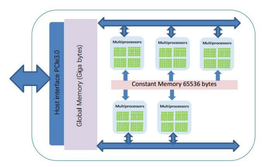
IP pair will be copied to GPU’s global memory by PCI-E bus. A IP pair buffer on GPU memory, which can contain $\alpha$ IP pairs, is allocated to receiving IP pairs. When the buffer is full or IP pairs in a slot are all copied, the same number of threads, as the number of receiving IP pairs, will be launched on GPU to process these IP pairs. Every thread reads one IP pair from global memory and update a distance recorder in RSRA which locating in global memory too. For IP v4 address, the buffer of IP pair occupies $8*\alpha$ bytes. When $\alpha$ is set to $2^{15}$, this buffer needs 256 KB memory. The graphic memory on GPU, ranging from 1 GB to 11 GB, is big enough to hold it. Although the RSRA requires more memory than IP pair buffer, the global memory is plenty enough to store a RSRA which is big enough for a 40 Gb/s networks. Other running parameters, such as hash function parameters, r, q and $\delta$, are stored in the constant memory which is read only but has high speed. A low cost GPU, which can be brought within 200 dollars, is fast enough to scan IP pairs in 40 Gb/s in real time. RSRA could be deployed in many nodes at different places to processes packets in the distributing environment. Every node should maintain the same size $RSRA$ and same hash functions’ parameters.

After scanning all IP pairs in a slice, sliding super point will be reconstructed from RSRA. If there are many nodes in the distributing environment, $RSRA$ in these nodes should be merged to a global one by $SRE$ merging and sliding super point will be detected from this global $RSRA$. According to the feature of RHFG, if $RSRA(aip)$ is known, $aip$ could be restored from it. But $RSRA(aip)$ is not stored directly. According to the definition, if $aip$ is a sliding super point, every sliding rough estimator in $RSRA(aip)$ will contain no less than $\eta*\rho$ short integers whose value is smaller than $k$. The sliding rough estimator whose weight is no less than $\eta*\rho$ is called as hot sliding rough estimator denoted by $HSE$.

A candidate tuple $CT$ consists of r $HSE$s could be acquired by selecting a $HSE$ from every $HSE(i)$ where $0\leq i\leq r-1$. $CT=\{he_{0},he_{1},he_{2},\cdots,he_{r-1}\}$ where $he_{i}\in HE(i)$. Sliding super point could be regained by testing all of these candidate tuples.

Two additional buffers of candidate tuples are used in this algorithm, one for storing and the other for reading. Their roles exchange in different levels when adding hot estimators in different rows. Let $SCTB$ point to the candidate tuple buffer for storing and $RCTB$ point to the candidate tuple buffer for reading.

Candidate tuple in these two buffers grows incrementally from empty to a valid tuple containing $r$ hot estimators in different rows. Let $CTB_{1}$ and $CTB_{2}$ represent these two buffers respectively. Figure 4 shows how candidate tuple grows with two buffers’ support.

These two candidate tuple buffers are located on GPU’s global memory. Candidate tuple $CT_{2}=\{he_{0},he_{1},he_{2}\}$ with three hot estimators, selected from $HSE(0)$, $HSE(1)$, $HSE(2)$ separately, will be inserted into $CTB_{1}$ after checking. The checking procedure is to test if $B(1)$ and $B(2)$ extracted from $CT_{2}$ is valid, if the left $q-\delta$ bits of $B(1)$ is the same as the right $q-\delta$ bits of $B(2)$. Only when passing the test, will $CT_{2}$ be added to $CTB_{1}$. When $q-\delta$ is big, only a small part of such candidate tuple will appear in $CTB_{1}$. The memory updating latency caused by candidate tuple insertion will be concealed by the huge parallel running threads on GPU. So candidate tuple checking determines the time consumption of a thread. When every thread deals with the same amount of candidate tuples, they will finish approximately at the same time. In this situation, the load of every thread is balance and GPU realizes its full potential.

There are total $Q=|HSE(0)|*|HSE(0)|*|HSE(0)|$ candidate tuples like $CT_{2}$. Suppose $V$ threads are launched on GPU to deal with these candidate tuples. Let $U$, $V$, $Q$ and $W$ be non-negative integers. In order to let every thread has the same candidate tuples to check, each thread will be assigned at least $U=Q/V$ candidate tuples evenly. Still there are $W=Q\ mod\ V$ candidate tuples rest. In these $V$ threads, every of first $W$ threads has $U+1$ candidate tuple and every of the rest $V-W$ threads has $U$ candidate tuple. Let $CT_{2}(i)$ represent the set of candidate tuples to be tested by the $i$th threads in GPU which can be acquired from $HSE(0)$, $HSE(1)$, $HSE(2)$. Algorithm 4 shows how every thread checks candidate tuples.

$CT_{2}(TID)$ could be acquired from $HSE(0)$, $HSE(1)$, $HSE(2)$ according to the index of a GPU thread. When testing candidate tuple in $CTB_{2}(TID)$, valid candidate tuple which passes checking process from line 9 to 11 will be stored in $SCTB$ for further checking with hot estimators in other rows.

When all threads finished, $CTB_{1}$ which has stored all valid candidate tuples extracting from the first three rows will work as reading buffer and the other buffer, $CTB_{2}$ will be used for storing new candidate tuple as shown in figure 4.

For $HSE(i)$ where $i\geq 3$, a new candidate tuple for checking is generated from a candidate tuple in reading tuple buffer, candidate tuple buffer which has stored valid candidate tuple, and a hot estimator in it. Then $Q=|RCTB|*|HSE(i)|$ where $|RCTB|$ means the number of candidate tuple storing in reading candidate tuple buffer. When $i$ is an odd number, $RCTB$ points to $CTB_{1}$, $SCTB$ points to $CTB_{2}$; when $i$ is an even number, $CBT_{1}$ and $CBT_{2}$ exchange roles. A new candidate tuple consists of a hot estimator in $HSE(i)$ and a candidate tuple in $RCTB$. The set of such new candidate tuple to be checked by the $j$th thread, $CT_{i}(j)$, could be generated from $HSE(i)$ and $RCTB$. Algorithm 5 shows how to check new candidate tuples.

When checking a candidate tuple newly adding a hot estimator in $HSE(i)$, only $B(i-1)$ and $B(i)$ should be tested. After update candidate tuple with the last row, $SCTB$ contains candidate tuple from which a valid host could be reconstructed. Set $Q=|SCTB|$, $U=\frac{Q}{V}$ and launch $V$ threads. Every thread scans $U$ or $U+1$ reconstructed hosts to estimate their opposite number according their union sliding estimators in the candidate tuple and check if they are sliding super points. By this method, every thread on GPU has the similar load with the cost of additional buffers for storing middle candidate tuples. Nowadays GPU has plenty global memory and the buffers not occupy many space because the number of sliding super points takes up a small part of hosts.

$RSRA$ reconstructs sliding super points fast on GPU. But it can’t get their cardinality and some fake host may hide in the candidate list. This problem will be solved by the method proposed in the next section.

References

- [1] Cisco. Global ip traffic forecast. http://www.cisco.com/c/en/us/solutions/collateral/service-provider/visual-networking-index-vni/vni-hyperconnectivity-wp.pdf, 2017. Online.
- [2] Monowar H. Bhuyan, D.K. Bhattacharyya, and J.K. Kalita. Surveying port scans and their detection methodologies. Comput. J., 54(10):1565–1581, October 2011.
- [3] Mansour Alsaleh and P. C. van Oorschot. Network scan detection with lqs: A lightweight, quick and stateful algorithm. In Proceedings of the 6th ACM Symposium on Information, Computer and Communications Security, ASIACCS ’11, pages 102–113, New York, NY, USA, 2011. ACM.
- [4] Poonam Sinai Kenkre, Anusha Pai, and Louella Colaco. Real Time Intrusion Detection and Prevention System, pages 405–411. Springer International Publishing, Cham, 2015.
- [5] Martin Roesch. Snort - lightweight intrusion detection for networks. In Proceedings of the 13th USENIX Conference on System Administration, LISA ’99, pages 229–238, Berkeley, CA, USA, 1999. USENIX Association.
- [6] S. Karthik and J. J. Shah. Analysis of simulation of ddos attack in cloud. In International Conference on Information Communication and Embedded Systems (ICICES2014), pages 1–5, Feb 2014.
- [7] Jelena Mirkovic and Peter Reiher. A taxonomy of ddos attack and ddos defense mechanisms. SIGCOMM Comput. Commun. Rev., 34(2):39–53, April 2004.
- [8] S. T. Zargar, J. Joshi, and D. Tipper. A survey of defense mechanisms against distributed denial of service (ddos) flooding attacks. IEEE Communications Surveys Tutorials, 15(4):2046–2069, Fourth 2013.
- [9] J. Mirkovic, G. Prier, and P. Reiher. Attacking ddos at the source. In 10th IEEE International Conference on Network Protocols, 2002. Proceedings., pages 312–321, Nov 2002.
- [10] Chenfeng Vincent Zhou, Christopher Leckie, and Shanika Karunasekera. A survey of coordinated attacks and collaborative intrusion detection. Comput. Secur., 29(1):124–140, February 2010.
- [11] Shobha Venkataraman, Dawn Song, Phillip B. Gibbons, and Avrim Blum. New streaming algorithms for fast detection of superspreaders. In in Proceedings of Network and Distributed System Security Symposium (NDSS, pages 149–166, 2005.
- [12] J. Cao, Y. Jin, A. Chen, T. Bu, and Z. L. Zhang. Identifying high cardinality internet hosts. In IEEE INFOCOM 2009, pages 810–818, April 2009.
- [13] Guang Cheng and Yongning Tang. Line speed accurate superspreader identification using dynamic error compensation. Computer Communications, 36(13):1460 – 1470, 2013.
- [14] P. Wang, X. Guan, T. Qin, and Q. Huang. A data streaming method for monitoring host connection degrees of high-speed links. IEEE Transactions on Information Forensics and Security, 6(3):1086–1098, Sept 2011.
- [15] W. Liu, W. Qu, J. Gong, and K. Li. Detection of superpoints using a vector bloom filter. IEEE Transactions on Information Forensics and Security, 11(3):514–527, March 2016.
- [16] Kyu-Young Whang, Brad T. Vander-Zanden, and Howard M. Taylor. A linear-time probabilistic counting algorithm for database applications. ACM Trans. Database Syst., 15(2):208–229, June 1990.
- [17] Shane Ryoo, Christopher I. Rodrigues, Sara S. Baghsorkhi, Sam S. Stone, David B. Kirk, and Wen-mei W. Hwu. Optimization principles and application performance evaluation of a multithreaded gpu using cuda. In Proceedings of the 13th ACM SIGPLAN Symposium on Principles and Practice of Parallel Programming, PPoPP ’08, pages 73–82, New York, NY, USA, 2008. ACM.
- [18] John E. Stone, David Gohara, and Guochun Shi. Opencl: A parallel programming standard for heterogeneous computing systems. IEEE Des. Test, 12(3):66–73, May 2010.
- [19] Seon-Ho Shin, Eun-Jin Im, and MyungKeun Yoon. A grand spread estimator using a graphics processing unit. Journal of Parallel and Distributed Computing, 74(2):2039 – 2047, 2014.
- [20] Piotr Indyk. A small approximately min-wise independent family of hash functions. Journal of Algorithms, 38(1):84 – 90, 2001.
- [21] Daniel M. Kane, Jelani Nelson, and David P. Woodruff. An optimal algorithm for the distinct elements problem. In Proceedings of the Twenty-ninth ACM SIGMOD-SIGACT-SIGART Symposium on Principles of Database Systems, PODS ’10, pages 41–52, New York, NY, USA, 2010. ACM.
- [22] Mihai Patrascu and Mikkel Thorup. The power of simple tabulation hashing. In Proceedings of the Forty-third Annual ACM Symposium on Theory of Computing, STOC ’11, pages 1–10, New York, NY, USA, 2011. ACM.
- [23] Center for Applied Internet Data Analysis. The caida anonymized internet traces. http://www.caida.org/data/passive, 2017. Online;accessed 2017.