On semi-supervised learning
Alejandro Cholaquidisa, Ricardo Fraimana and Mariela Sued b
a CABIDA and Centro de Matemática,
Facultad de Ciencias, Universidad de la República, Uruguay
b Instituto de Cálculo,
Facultad de Ciencias Exactas y Naturales, Universidad de Buenos Aires
Semi-supervised learning; Small training sample; Consistency.
Abstract
Semi-supervised learning deals with the problem of how, if possible, to take advantage of a huge amount of unclassified data, to perform a classification in situations when, typically, there is little labeled data. Even though this is not always possible (it depends on how useful, for inferring the labels, it would be to know the distribution of the unlabeled data), several algorithm have been proposed recently.
A new algorithm is proposed, that under almost necessary conditions, attains asymptotically the performance of the best theoretical rule as the amount of unlabeled data tends to infinity. The set of necessary assumptions, although reasonable, show that semi-supervised classification only works for very well conditioned problems. The focus is on understanding when and why semi-supervised learning works when the size of the initial training sample remains fixed and the asymptotic is on the size of the unlabeled data. The performance of the algorithm is assessed in the well known “Isolet” real-data of phonemes, where a strong dependence on the choice of the initial training sample is shown.
1 Introduction
Semi-supervised learning (SSL) dates back to the 60’s, starting with the pioneering works of Scudder (1965), Fralick (1967) and Agrawala (1970), among others. Later on, the problem was addressed by the highly influential works of Castelli and Cover (1995); Castelli and Cover (1996). The first one shows that when the size of the unlabelled sample is equal to infinity, the classification error converges exponentially fast to the Bayes risk, if the size of the labelled sample converges to infinity. In the second one it is assumed that the density of the covariates is given by a parametric model , where is known except for the parameters and . Under regularity conditions consistency is shown if the minimum between and converges to infinity.
Recently SSL has gained paramount importance due to the huge amount of data coming from diverse sources, such as the internet, genomic research, text classification, and many others; see, for instance Zhu (2008) or Chapelle, Schölkopf and Zien, eds. (2006) for a survey on SSL. This large amount of data is typically unlabelled; the main purpose of SSL is to jointly classify these data in the presence of a small “training sample”. Namely, a lot of unlabelled data together with a small quantity of labelled data must be combined to classify each unlabelled observation. As in Arnold et al (2007) “A setting that is closely related to semi-supervised learning is transductive learning Vapnik (1998); Joachims (1999); Joachims (2003)”, which is a special case of SSL, where the auxiliary unlabelled data-set coincides with the test sample. On the other hand, from a transductive learning procedure any other data point can be classified with any machine learning algorithm, by using as training sample the output of the transductive procedure.
On the other hand, as discussed in Chapelle, Schölkopf and Zien, eds. (2006), the following question naturally arises: “in comparison with a supervised algorithm that uses only labelled data, can one hope to have a more accurate prediction by taking into account the unlabelled points? […] In principle, the answer is yes”. Nevertheless, having a large set of data to classify is like knowing , the distribution of the features vector; thus, the gain in prediction accuracy depends on the ability of to provide information on . As it is pointed in Chapelle and Zien (2005), “the cluster assumption is key to successful semi-supervised learning”, which is expressed in terms of the so called valley condition. Roughly speaking, this condition imposes to have a deep valley between the classes. In other words, clustering techniques have to perform reasonably well in the presence of only unlabelled data. Smoothness of the labels with respect to the features, or low density at the decision boundary, are examples of the kind of hypotheses required to get satisfactory results in the cluster analysis literature.
Another important issue in SSL is the amount of labelled data necessary to be able to classify the unlabelled data. In the framework of generative models,
when is assumed to be an identifiable mixture of parametric distributions, Zhu (2008) argued that “ideally we only need one labelled example per component” to fully determine the mixture distribution. Indeed, under the regularity conditions presented in Section 5, one labelled example per component will also be enough to prove the consistency of the algorithm that we propose in this work.
Recently, other approaches as self-training, co-training, transductive support vector machines, and graph-methods among others, have been reported. Although there is a large body of literature on SSL, as it is pointed out by Azizyan et al. (2013), “making precise how and when these assumptions actually improve inferences is surprisingly elusive, and most papers do not address this issue; some exceptions are Rigollet (2007), Singh et al. (2008), Lafferty and Wasserman (2007), Nadler et al. (2009), Ben-David et al. (2008), Sinha and Belkin (2009), Belkin and Niyogi (2004), Vapnik (1998), Wang et al. (2007) and Niyogi (2008)”. In Haffari and Sarkar (2007) the well known Yarowski algorithm is analyzed, while in Azizyan et al. (2013) an interesting method called “adaptive semi-supervised inference” is introduced, and a minimax framework for the problem is provided.
Our proposal is focused on the case of a small and fixed training sample size, but the amount of the unlabelled data goes to infinity (see Figure 1). We provide a simple algorithm to classify the unlabelled data, which has a resemblance to Yarowski’s formulation. We prove that, under some natural and necessary conditions (some of them are in terms of well–known geometric constraints on the support of coming from stochastic geometry), our method performs as good as the theoretical (unknown) best rule, with probability one, asymptotically in . These conditions are discussed in Section 8 where we argue that most of them seems to be necessary.
The algorithm is of the “self-training” type; this means that at every step a point from the unlabelled set is labelled using the training sample built up to that step, and incorporated into the training sample. In this way the training sample increases from one step to the next. A simplified, computationally more efficient alternative algorithm is also provided in Section 6.
This paper is organized as follows: Section 2 introduces the basic notation and the set-up necessary to read the rest of the article. Section 3 proves that the Bayes rule is the best one to classify the unlabelled sample. In Section 4 we introduce the algorithm and prove that all the unlabelled data are classified. Section 5 proves that, as the number of unlabelled data grows to infinity, the algorithm performs as good as Bayes rule. In Section 6 we introduce a simplified and faster algorithm. Section 7 analyses two examples using simulated data, and a third one based on a real data set. Lastly, Section 8 discusses the hypotheses. The proofs are included in Appendixes A and B.
2 Notation and set-up
Along this work we use to denote probability events, namely, subsets of a (rich enough) probability space . Instead are used to denote subsets in the Euclidean space . In most of the cases, the probability events are defined through conditions on the random variables that concern . We use the same letter in different styles with the hope to facilitate the reading of the work.
We consider endowed with the Euclidean norm . The open ball of radius centered at is denoted by . With a slight abuse of notation, if , then we write . The -dimensional Lebesgue measure is denoted by , while . For and , the -interior of is defined as . The distance from a point to a set is denoted by , i.e. . If , then denotes its boundary, its interior, its complement, and its closure. Let be a given realization of a sample with the same distribution as , where . We assume that they are identically distributed but not necessarily independent. Let denote the conditional mean of given ; namely, . Consider an iid sample with the same distribution as , where . The sample is known while the labels are unobserved.
3 Theoretical best rule
It is well known that the optimal rule for classifying a single new datum is given by the Bayes rule, . In the present paper, we move from the classification problem of a single datum to a framework where each coordinate of must be classified. The label associated with each coordinate may be constructed on the basis of the entire vector and, therefore, a classification rule comprises functions , where indicates the label assigned to based on the entire set of observations . The performance of a rule is given by its mean classification error, namely Observe that the random variable is not necessarily for some .
The next result establishes that the optimal classification rule classifies each element ignoring the presence of the rest of the observations, by means of invoking the Bayes rule.
Proposition 1.
The performance of a rule is bounded from below by , and the lower bound is attained with the rule , where for all .
In practice, since the distribution of is unknown, an estimator of may be defined by a sequence , where indicates the label to be assigned to the element . In what follows we try to find a sequence , such that
| (1) |
where denotes the expectation wrt .
Remark 1.
It can be surprising that the limit in display (1) does not depend explicitly on the size of the initial training sample . Our purpose is to analyze under which conditions such a strong statement can be derived. As it is proved in Theorem 1, the initial training sample must be well located in the sense of assumption H8 given below. Moreover, strong but almost necessary assumptions discussed in Section 8 are required to get the desired result.
Next section presents an algorithm that, under several conditions (given in section 5), satisfies a stronger property. More precisely, we will show that
where and is the step of the algorithm at which the point is classified.
4 Algorithm
We provide an algorithm which is asymptotically optimal in the sense of satisfying condition (1). For this purpose, we update the training sample sequentially incorporating into the initial set an observation in with a predicted label . At each step we choose the point whose score to predict its label is as extreme as possible, as stated in display (3). Scores are constructed according to the majority rule in a neighborhood of the corresponding observations to be classified; i.e., we estimate with a Nadaraya-Watson estimator using a uniform kernel, based on both and those points already classified by the algorithm up to the present step. In this way we choose the “best classifiable point” from those that remain unclassified, as indicated in the following recipe:
- Initialization:
Let , , .
- STEP :
For in , choose the best classifiable point in , from those that are at a distance smaller than from the points already classified, as follows: let ; for , consider
(2) (3) If there is more than one satisfying (3), choose one that maximizes
(4) Then label with defined by , where is the classification rule associated with defined in (2). Namely, . Consider
- OUTPUT:
.
Alternatively, to reduce the computational time, in Step , instead of choosing only one point satisfying (3) and maximizing (4), it is possible to choose, among the points that satisfy (3), all those fulfilling (4). More precisely, we define as the set of all the points that satisfy (3) and that maximize . Then we label with defined by for all , where is the classification rule associated with defined in (2). More precisely, . Lastly
The results discussed in the remainder of this work hold for both versions of the algorithm. To simplify the notation, they are only presented for the first version, labelling one point at each step. However, the data analysis developed in Section 7 is based on the second version of the algorithm.
We will now prove that the algorithm classifies the whole set . For that purpose, define and assume that and are connected and coverable, as stated in condition H3 below. Observe that , where is assumed to be the support of the random vector . We decided to include H3 to facilitate the proof of Proposition 2. In Proposition 3 we will provide sufficient conditions which guarantee the validity of H3. Such conditions are expressed in terms of geometric restrictions on , , regularity assumptions on the density function of the distribution of , and on the rate at which the bandwidth decreases to zero. These conditions will also be discussed in Section 8. Additionally, we require to have at least one point of the training sample in , for . To be more precise, consider the following assumptions:
- H1.
.
- H2.
For , is connected, and
- H3.
The covering property: the probability event fulfills , for , where,
- H4.
There exists in such that , for .
In the sequel, we will assume H1 and therefore . We can now establish that, for large enough, the algorithm assigns labels to each point in .
Proposition 2.
Assume , i), and . Then, with probability one, for large enough, all the points in are classified by the algorithm: , where and, for , .
Remark 2.
If we estimate with a -nearest neighbor rule instead of the kernel procedure proposed in this work, the result presented in Proposition 2 holds with no assumptions.
More generally, in the algorithm might be replaced by other local nonparametric regression estimator like neural networks. However, among other conditions, the diameter of the partition cells will play an important role. The analysis of consistency of the proposed algorithm based on -nn or neural network rules is beyond the scope of this manuscript.
5 Consistency of the algorithm
To prove the consistency of the algorithm additional conditions are required. They involve regularity properties of different sets and the rate at which decreases. Define the following sets, illustrated in Figure 9:
Besides H1-H4 introduced in Section 4, we will also assume that both the -interior and of and , respectively, are connected and coverable, as stated in H5. This hypothesis (as we will see in Appendix B) is fulfilled if we assume that the set , , has positive reach, (as introduced in Federer (1959)) and . Assumption H7 holds if , as it is proved in Abdous and Theodorescu (1989). Moreover, the density of the distribution of needs to take larger values on the interiors than on the borders , as indicated in H6. Finally, all the labels in the training set must agree with those determined by the Bayes’s rule, apart from being well located, as presented in H8. Namely, consider the following set of hypotheses, which will be discussed in Section 8:
- H5.
There exists such that, for and for any , is connected, and the probability event fulfills , where
(5) for .
- H6.
The Valley Condition: The probability function induced by has a density verifying that exists such that for all there is , such that when
(6) - H7.
The kernel density estimator converges to uniformly over its support , almost surely:
(7) - H8.
Good training set: for all ; moreover, there exists in such that , for , for some . Observe that H8 implies H4.
Even if no condition is imposed on the bandwidth , the algorithm implicitly assumes that it converges to zero. Indeed, in Proposition 3, we ask for rates of convergence to guarantee the validity of condition H3, H5 and H7, aside from
some regularity conditions on and the sets for .
Following the notation in Federer (1959), let be the set of points with a unique projection on , denoted by . That is, for , is the unique point that achieves the minimum of for . For , let reach. The reach of is defined by and is said to be of positive reach if .
Proposition 3.
Assume that H2 i) and ii) hold and that is compact supported, continuous, bounded from below by a positive constant. Assume also that , for . The bandwidth fulfills and . Then H3, H5 and H7 hold.
The main result of this work is presented in Theorem 1; it states that the algorithm proposed in Section 4 is consistent, in the sense defined in (1). To prove this result, we will invoke the following preliminary lemmas. The first of them, Lemma 1, establishes that the first point classified differently from the Bayes rule is in the boundary region . Then, in Lemma 2, we combine the valley condition with the uniform consistency of the kernel estimator to show that, asymptotically, there are more points of in than in . Lemma 3 states that all the points far enough from the boundary region are labeled by the algorithm, with the same label that the one given by the Bayes rule. To be more precise, recall that, and define
Look at the first time, , where the algorithm assigns a label different from that prescribed by the Bayes rule, if such a step exists; otherwise, define . Namely,
| (8) |
From now on, we will say that a point is badly classified whenever ; otherwise the point will be called well classified. The next result establishes that is in .
Lemma 1.
Assume that H1 and H8 hold. Then,
Lemma 2.
Assume H6 and H7. Then, , for any where
Lemma 3.
Assume H1–H8. Then, for any
| (9) |
and therefore, on , we have that
| (10) |
6 A faster algorithm
The algorithm given in Section 4 classifies a few points of at each step. This can be discouraging when is too large. In order to overcome this issue, we will introduce a simple modification that gives rise to a faster procedure in terms of computational time (see Table 3), at the expense of introducing a small increment in the classification error rate (this increment can be controlled but with computational cost).
The idea is to pre-process the sample , and project it on a grid , as we describe in what follows. We can assume, without loss of generality, that with . For fixed, to be determined by the practitioner, consider for . The -grid on is determined by the points of the form with , for . Each point in the grid determines a cell
Given , let be the set of points in the grid whose corresponding cell intersects ; now project (or collapse) on , in the sense that the algorithm will be applied to in lieu of . Then, all the points in will be classified with the label assigned to by the algorithm.
7 Examples with simulated and real data
In this section we report some numerical results, comparing the performance of the SSM algorithm presented in Section 4 and its faster version, introduced in Section 6, with that of other supervised algorithms. Specifically, -nearest neighbors (-nn) and support vector machines (SVM) are the supervised techniques used to assign labels of each element in on the basis of the training sample .
The classification error rate of each algorithm is computed in three scenarios. In the first two, we use artificially generated data, whereas in the last one we employ a real data set. The first example compares efficiency of the three algorithms (-nn, SVM and the SSL algorithm introduced in section 4). The second one shows the effect of the grid size with respect to classification error rate and computational time. The third one is a well known real-data set where we illustrate the crucial effect of the initial training sample .
7.1 A first simulated example
The joint distribution of is generated as follows: consider first the curve in the square , defined by . All the points in the square that are below will be labeled with while those that are above the curve will be labeled with . Now, to emulate the valley condition, those points close to will be chosen with less probability than those far away. To do so, let and denote the set of points in the square which are at -distance larger / smaller than from , respectively. Namely, and , where is the supremum norm. Let , and be independent random variables, with , and . Consider the random variable , while if and if .
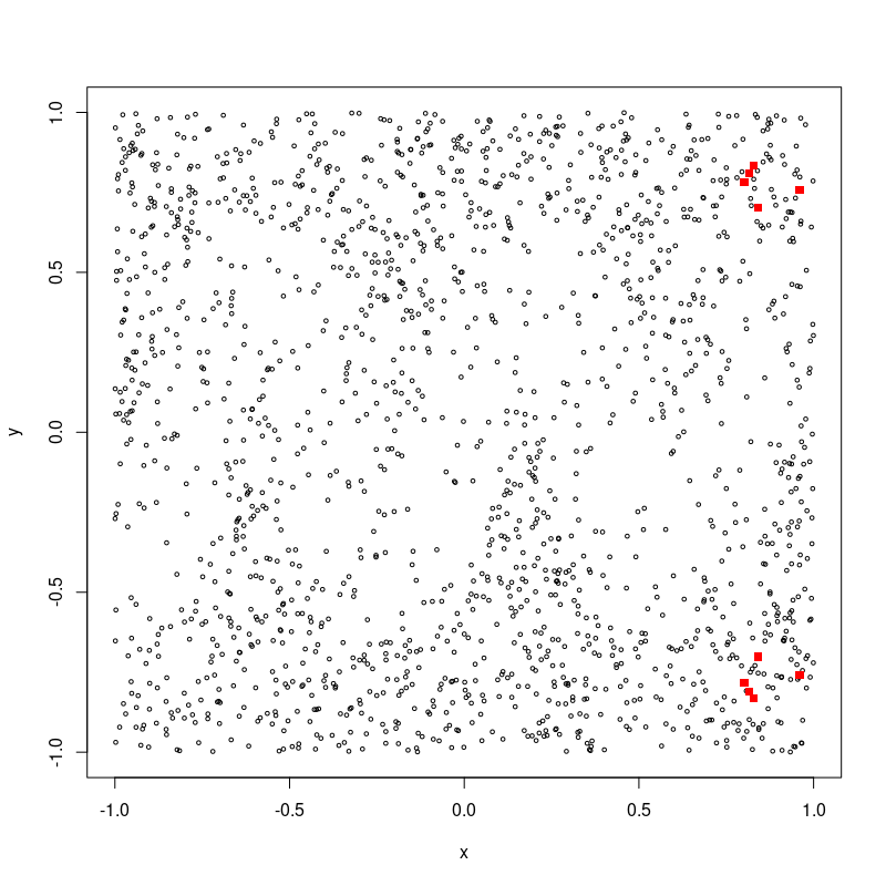
We first study the performance of our algorithm, analyzing the error rates among 50 replications of the described scheme, with , and . An histogram of the classification errors is presented on the right panel of Figure 2 and a summary is reported in Table 1. There are four out of the fifty replications where the classification errors are much higher than in the other cases. These extreme results can be attributed to the initial training sample (see assumption H8). The initial training sample for the best and the worst case (in terms of classification error rate) are also shown on the left panels of Figure 2.


| Min. | 1st Qu. | Median | Mean | 3rd Qu. | Max. |
| 0.0179 | 0.0267 | 0.0365 | 0.0458 | 0.0469 | 0.1554 |
Next, we compare the misclassification error of the semi-supervised methods introduced in this work with that of some supervised classification algorithms trained with to label . -nn is, naturally, the first method to be considered. As often happens in the presence of a tuning parameter, the choice of may impact on the performance of the procedure. In particular, in the present scenario, will be chosen on the base of the training set , with , which may turn in an unstable recipe to select . To analyze the distribution of in such a situation, we generated 1000 samples of and for each of them we computed . The results are shown in Figure 3.

The three more frequent values of ( and ) were used to classify with a -nn method trained with . The mean error rates among 1000 replications are given in Table 2. It is worth to mention that the error rates of SSL and -nn are computed with 50 and 1000 replications, respectively. This is due to computational demands of each procedure.
| Min. | 1st Qu. | Median | Mean | 3rd Qu. | Max. | |
|---|---|---|---|---|---|---|
| 0.026 | 0.076 | 0.097 | 0.104 | 0.123 | 0.289 | |
| 0.034 | 0.091 | 0.114 | 0.124 | 0.147 | 0.368 | |
| 0.052 | 0.108 | 0.129 | 0.142 | 0.163 | 0.448 |
Finally, we kept and vary , choosing , with . At each of the steps, new unlabelled data are included to conform the set . Four competitors were considered: -nn with chosen by cross validation, support vector machine (SVM, using the package LIBSVM in julia 1.2), both of them trained with , and our SSL proposal with and . The whole procedure is repeated times. In figure 4 we plot the median, mean, 0.25, and 0.75 quantile of the misclassification errors respectively. As expected, the misclassification errors for -nn and SVM remain mainly constant, while the misclassification error of the SSL algorithm decreases with . Observe that for around 500 the SSL algorithm outperforms its competitors.


Figure 5 exhibits the labels assigned by four different methods to a fixed realization of both and . In the first row we show the labels assigned by the algorithm (with ), and the fast version of it. In the second row, the labels assigned by -nn, with =7 and SVM. The classification error rates corresponding to each method are , , and , respectively.


7.2 A second example using simulated data
To generate the data consider two bi-variate normal random vectors and . Let . The conditional distribution of given , for , is given by .
We consider two cases: , (see Figure 6 left) and , (see Figure 6 right); in both cases . In the first case the Bayes error is and in the second one is .
We generate iid, with distributed as , and sample size . In each replication, we used and bandwidth to run the algorithm.
The average of the computational time as well as the error rate over 50 replications are reported in Table 3, for different grid sizes. As it is shown in Table 3, there is a trade-off between computation time and efficiency. However, if the cell sizes of the grid are reasonably small (as in the first column of Table 3), the misclassification errors are essentially the same, while the computational time decreases. The simulation was performed in Julia 1.0.1, running on an Intel i7-8550U.


| Without Grid | Grid step 0.1 | Grid step 0.15 | |||
| First Case | |||||
| Time | Error | Time | Error | Time | Error |
| 4.2s | 0.0323 | 2.8s | 0.043 | 1.1s | 0.046 |
| Second Case | |||||
| Time | Error | Time | Error | Time | Error |
| 5.15s | 0.084 | 2.7s | 0.10 | 0.98s | 0.117 |
7.3 A real data example
We consider the well known Isolet data set of speech features from the UCI Machine Learning Repository Asuncion and Newman (2007), comprising 617 attributes associated with the English pronunciation of the 26 letters of the alphabet. The data come from 150 people who spoke the name of each letter twice. There are three missing data, not considered in the study. Feature vectors include: spectral coefficients, contour features, sonorant features, pre-sonorant features, and post-sonorant features, and are described in Fanty and Cole (1991). The spectral coefficients account for 352 of the features. The exact order of appearance of the features is not known.
We apply the semi-supervised algorithm to the binary problem given by the E-set comprising the letters and the R-set with the remaining letters except for the letters , starting with a small labelled data set of 10 elements from each group. Then consists of data.
To pre-process the data, we first removed the first repetition of every letter. Next, we kept only those data whose nearest neighbour is at a distance smaller than a threshold (the value was selected to reduce the misclassification error, and to reduce the computational time, in order repeat it 100 times). This pruning procedure reduced the sample to data. To study how the misclassification error varies with respect to the training sample, we randomly chose a training sample 100 times. We compared with -nn choosing by cross validation, using replicates. A summary of the misclassification error rates is shown in Figure 7 right, while the density of the errors of SSL is shown in Figure 7 left.
![[Uncaptioned image]](1805.09180v3/densityerr.png)
| Min. | 1st Qu. | Median | Mean | 3rd Qu. | Max. | |
|---|---|---|---|---|---|---|
| SSL | 0.028 | 0.076 | 0.139 | 0.130 | 0.184 | 0.247 |
| -nn | 0.048 | 0.124 | 0.149 | 0.144 | 0.168 | 0.216 |
8 Some remarks regarding the assumptions
We discuss briefly the set of assumptions considered. Firstly, we would like to point out that the results we are looking at are quite strong, since the training sample is frozen at a small fixed size and the asymptotic is on the unlabeled data size. These results should not be misinterpreted. Without these hypotheses, the semi-supervised classification methods may work better than the classical supervised classification methods but the consistency will not be verified if the size of the training sample remains fixed.
- 1)
In order for an algorithm to work for the semi-supervised classification problem, the initial training sample (whose size does not need to tend to infinity) must be well located. We require that satisfies for all , which is a quite mild hypothesis. In many applications, a stronger condition can be assumed. For instance, if the two populations are sick or healthy, the initial training sample can be chosen as the set of individuals for whom the covariate ensures the condition on the patient, that is, or . On the other hand, if the initial training sample is not well located, then any algorithm might classify almost all observations wrongly. Indeed, consider the case where the distribution of the population with label 0 is and the other is . This will be the case if we start for instance with the pairs .
The effect of the initial training sample is illustrated in the real-data example where the misclassification error varies between 0.028 and 0.247 by changing at random . - 2)
The connectedness of and is also critical. In a situation like the one shown in Figure 8, the points in the connected component for which there is no point in (represented as squares) will be classified as the circles by the algorithm. However, if and have a finite number of connected components and there is at least one pair in each of them with , it is easy to see that the algorithm will be consistent.
- 3)
The uniform kernel assumption can be replaced by any regular kernel satisfying for some positive constants , and the results still hold.
- 4)
In Proposition 3 we assume that has a continuous density with compact support . If that is not the case, it is possible to take a large enough compact set such that is very small and therefore just a few data from is left out.
- 5)
The following example shows that H5 is necessary for consistency. Indeed, suppose that and with , then for all , . Unless the training sample contains two points and with and very close to , semi-supervised methods will fail. Regardless of the value of , the classes 0 and 1 are indistinguishable since the joint distribution is in all cases .
Moreover, there is no consistent semi-supervised algorithm for fixed. To see this, consider a training sample in with fixed size . Let us denote , , and the labels assigned by any algorithm. Then if , conditioned to the training sample , if we choose we will miss-classify at least data-points, and if , we will do the same.

9 Concluding remarks
In this paper we address the problem of semisupervised learning. We propose a simple algorithm and analize its asymptotic behaviour.
The focus is on understanding when and why SSL works when the training sample is small and frozen, and the asymptotic is in the sense of the strong formulation given in equation (1), where the limit is only on the size of the unlabelled data-set.
From the discussion on Section 8 it follows that SSL will only work under the almost necessary hypotheses we have assumed.
The first simulation example shows the behaviour of our algorithm. In particular Figure 2 and Table 1 exhibit the effect of the initial training sample on the output of the procedure, which is related to assumption H8. We also study the effect of increasing the size of the unlabelled data, where we compare with two well known competitors: -nearest neighbours and support vector machine. Our SSL proposal outperforms the competitors if is larger than .
The second simulated example studies the trade-off between computation time and efficiency. Lastly, on the real-data example we challenge our algorithm by comparing with the -nearest neighbour rule performed on . In this case the results are only slightly better.
Appendix A
Proof of Proposition 1.
Observe that , for . Thus,
and therefore,
showing that , for any . The lower bound is attained by choosing the th coordinate of
equal to . Moreover, the accuracy of equals that of a single coordinate; namely .
Proof of Proposition 2.
We will prove that if H1, H2 i) and H4 are satisfied, then
. Combining this inclusion with H3 we conclude that .
To prove that
, we will see that if
| (11) |
all the elements of are labeled by the algorithm. To do so, note that, by H4, there exists in such that , for . We will now prove that the algorithm starts. Since is in and (11) holds with , there exists with . In particular, and so . This guarantees that and hence the algorithm can start.
Assume now that we have classified points of . We will prove that there exists at least one point satisfying the iteration condition required at step : . By H1 we can assume that . Take such that . We will consider now two possible cases: (i) if , then and so, by (11), for some . Since is in and , we conclude that . Assume now that (ii) . Since is connected and (11) holds, the union of , with , is also a connected set and, therefore,
Finally, take
and such that
to conclude that .
Proof of Lemma 1.
By H1, we can assume that for all .
Assume first that , that is, , , and all the points labelled up to the step by the algorithm are well classified. Now, suppose by contradiction , which means that and thus, . This implies that
for all , contradicting the label assigned to according to the majority rule that is used by the algorithm.
Thus, , and so . Analogously, if , we deduce that .
Proof of Lemma 2.
Given , choose such that , for introduced in H6. We will prove is included in as far as and therefore, from (7), we conclude that .
Now, note that on , we get that and so, on , for and , Thus, on ,
when . This proves that , for such that .
Proof of Lemma 3.
When , . This fact implies that, on the event , the following identity holds: . Thus, to prove (9), we need to show that, for
We will argue by contradiction, assuming that there exists
for which . Invoking H8, and there exists . These facts guarantee that , and since we are working on , we get that
| (12) |
Next, we will argue that there exist such that . To do so, consider the following two cases:
- (i)
- (ii)
Assume now that . Since is connected, the union of balls given in (12) is connected, and then,
Thus, there exist and with , which implies that .
To finish the proof, we will show that such a should have been chosen by the algorithm to be labelled before , which implies that , contradicting that . This contradiction show that no such exists, as announced. Since , we get that , the set of candidates to be labelled by the algorithm at step . Indeed, since and , . Thus, implying that attains the maximum stated in (3). Invoking now Lemma 2, since while is in (see Lemma 1), we know that ; thus, should have been chosen before . This conclude the prof of the result.
Proof of Theorem 1
Recall that denotes the label assigned by the algorithm to the observation. The empirical mean accuracy of classification satisfies
Consider , and . Combining the results obtained in Proposition 2 and Lemma 2 with condition H5, we conclude that , for . By (10), on , we have that and therefore
Then, on , we have that and so
| (13) |
On the other hand,
From Lemma 3, on , , and therefore, on ,
By H2 ii), the last term in the previous display converges to zero when , and thus
| (14) |
Combining (13) and (14) we deduce the announced convergence. The consistency defined in (1) follows from the Dominated convergence theorem.
Appendix B
In this section we will prove that under , conditions , and holds if we impose some geometric restrictions on and . In order to make this Appendix self contained, we need some geometric definitions and also include some results which will be invoked.
First we introduce the concept of Hausdorff distance. Given two compact non-empty sets , the Hausdorff distance or Hausdorff–Pompei distance between and is defined by
Next, we define standard sets, according to Cuevas and Fraiman (1997) (see also Cuevas and Rodríguez-Casal (2004)).
Definition 1.
A bounded set is said to be standard with respect to a Borel measure if there exists and such that where denotes the Lebesgue measure on .
Roughly speaking, standardness prevents the set from having peaks that are too sharp.
The following theorem is proved in Cuevas and Rodríguez-Casal (2004)).
Theorem 2.
(Cuevas and Rodríguez-Casal (2004) ) Let be a sequence of iid observations in drawn from a distribution . Assume that the support of is compact and standard with respect to . Then
| (15) |
where , , and is the standardness constant introduced in Definition 1.
Remark 3.
Theorem 2 implies that, if we choose with , then for large enough. This in turn implies that if is connected, is connected.
As a consequence of Theorem 2, we get the following covering property that will be used to prove Proposition 2 and H5 alone Proposition 3.
Lemma 4.
Let be a sequence of iid observations in drawn from a distribution with support . Let , be compact and standard with respect to restricted to , with . Consider such that and . Then, with probability one, for large, where .
Proof.
We need to work with restricted to , in order to do that, consider the sequence of stopping times defined by and the sequence of visits to given by . Then, are iid, distributed as , with support . Observe that the distribution of is the restriction of to . Since is compact and standard wrt we can invoke Theorem 1 for , in order to conclude that there exists a positive constant depending on , such that for ,
| (16) |
where . Define now as the number of visits to the set up to time . Namely, By the law of large numbers, a.e., and therefore, for large enough, . Thus, by (16), recalling that , we get that
In particular,
∎
This last lemma will be applied to get the covering properties stated in H2 and H5 for and . The following results are needed to show that these sets satisfy the conditions imposed in Lemma 4.
Lemma 5.
Let be a distribution with support such that and . Assume that has density bounded from below by . Let such , then is standard with respect to , the restriction of to (i.e ), for all , with .
Proof.
Let . By corollary 4.9 in Federer (1959) applied to , we get that , and now by proposition 1 in Aaron, Cholaquidis and Cuevas (2017), is standard, with (see Definition 1). ∎
Lemma 6.
Let be a non-empty, connected, compact set with . Then for all , is connected.
Proof.
Let . By corollary 4.9 in Federer (1959) applied to , . Then, the function if , and if where denotes the metric projection onto , is well defined. By item 4 of theorem 4.8 in Federer (1959), is a continuous function, so it follows that is connected. ∎
Proof of Proposition 3.
Since (this follows from Proposition 1 and 2 in Cuevas, Fraiman and Pateiro-López (2012) together with Proposition 2 in Cholaquidis et al. (2014)), then . By Lemma 5, choosing , the set is standard with respect to restricted to , for . By Lemma 4, with , is coverable; finally we get that H3 is satisfied.
To prove H5 i) observe that the connectedness of follows from that of (H2 i) together with Lemma 6. For H5 ii), take small enough such that , which should exist because of H2 ii). By (1) in Erdös (1945), using that , we get that . Finally to prove the covering stated in H5 first observe that, by Lemma 5, is standard wrt restricted to . Invoking Lemma 4 with and recalling that we get the covering property stated in H5 iii).
Lastly the uniform convergence stated in H7 follows from Theorem 6 in Abdous and Theodorescu (1989), since is uniformly continuous, assumptions (i)-(iii) hold for the uniform kernel and the bandwidth fulfills .
Acknowledgments
We thank two referees and an associated editor for their constructive comments and insightful suggestions, which have improved the presentation of the present manuscript. We also thank to Damián Scherlis for helpful suggestions.
References
- Aaron, Cholaquidis and Cuevas (2017) Aaron, C., Cholaquidis, A., and Cuevas, A. (2017). Stochastic detection of some topological and geometric features. Electronic Journal of Statistics 11(2): 4596–4628. http://dx.doi.org/10.1214/17-EJS1370
- Abdous and Theodorescu (1989) Abdous, B. and Theodorescu, R. (1989). On the Strong Uniform Consistency of a New Kernel Density Estimator. Metrika 11: 177–194.
- Agrawala (1970) Agrawala, A.K. (1970). Learning with a probabilistic teacher. IEEE Transactions on Automatic Control 19: 716–723
- Arnold et al (2007) Arnold, A., Nallapati, R. and Cohen, W. (2007). A Comparative Study of Methods for Transductive Transfer Learning. Seventh IEEE International Conference on Data Mining Workshops (ICDMW )
- Asuncion and Newman (2007) Asuncion, A., and Newman, D.J. (2007). UCI Machine Learning Repository, http://www.ics.uci.edu/~mlearn/MLRepository.html, University of California, Irvine, School of Information and Computer Sciences
- Azizyan et al. (2013) Azizyan, M., Singh, A., and Wasserman, L. (2013). Density-sensitive semisupervised inference. The Annals of Statistics 41(2): 751–771.
- Belkin and Niyogi (2004) Belkin, M., and Niyogi, P. (2004). Semi-supervised learning on Riemannian manifolds. Machine Learning 56: 209–239.
- Ben-David et al. (2008) Ben-David, S., Lu, T. and Pal, D.(2008). Does unlabelled data provably help? Worst-case analysis of the sample complexity of semi-supervised learning. In 21st Annual Conference on Learning Theory (COLT). Available at http://www.informatik.uni-trier.de/~ley/db/conf/colt/colt2008.html.
- Chapelle, Schölkopf and Zien, eds. (2006) Chapelle, O., Schölkopf, B., and Zien, A., eds. (2006). Semi-Supervised Learning. MIT Press.
- Chapelle and Zien (2005) Chapelle, O. and Zien, A. (2005). Semi-Supervised Classification by Low Density Separation AISTATS Vol. 2005, pp. 57–64.
- Cholaquidis et al. (2014) Cholaquidis, A., Cuevas, A. and Fraiman, R. (2014). On Poincaré cone property. Ann. Statist., 42, 255–284.
- Castelli and Cover (1995) Castelli, V., and Cover, T. M. (1995). On the exponential value of labeled samples. Pattern Recognition Letters, 16(1), 105-111.
- Castelli and Cover (1996) Castelli, V., and Cover, T. M. (1996). The relative value of labeled and unlabeled samples in pattern recognition with an unknown mixing parameter. I EEE Transactions on information theory, 42(6), 2102-2117.
- Cuevas and Fraiman (1997) Cuevas, A., and Fraiman, R. (1997). A plug-in approach to support estimation. Annals of Statistics 25: 2300–2312.
- Cuevas and Rodríguez-Casal (2004) Cuevas, A., and Rodríguez-Casal, A. (2004). On boundary estimation. Adv. in Appl. Probab. 36: 340–354.
- Cuevas, Fraiman and Pateiro-López (2012) Cuevas, A., Fraiman, R. and Pateiro-López, B. (2012). On statistical properties of sets fulfilling rolling-type conditions. Adv. in Appl. Probab. 44 311–329.
- (1945) Erdös, P. (1945). Some remarks on the measurability of certain sets. Bull. Amer. Math. Soc. 51 728–731.
- Fanty and Cole (1991) Fanty, M., and Cole, R. (1991). Spoken letter recognition. In: R.P. Lippman, J. Moody, and D.S. Touretzky (Eds.), Advances in Neural Information Processing Systems, 3. Morgan Kaufmann, San Mateo, CA.
- Federer (1959) Federer, H. (1959). Curvature measures. Trans. Amer. Math. Soc. 93: 418–491.
- Fralick (1967) Fralick, S.C. (1967). Learning to recognize patterns without a teacher. IEEE Transactions on Information Theory 13: 57–64.
- Haffari and Sarkar (2007) Haffari, G. and Sarkar, A. (2007). Analysis of Semi-Supervised Learning with the Yarkowsky algoritm. Proceedings of the 23rd Conference on Uncertainty in Artificial Intelligence, UAI 2007. Vancouver, BC. July 19–22, 2007.
- Joachims (1999) Joachims, T. (1999). Transductive inference for text classification using support vector machines. In ICML 16 1999
- Joachims (2003) Joachims, T. (2003). Transductive learning via spectral graph partitioning. In ICML 2003
- Lafferty and Wasserman (2007) Lafferty, J., and Wasserman, L. (2008). Statistical analysis of semi-supervised regression. Conference in Advances in Neural Information Processing Systems. 801–808.
- Nadler et al. (2009) Nadler, B., Srebro, N., and Zhou, X. (2009). Statistical analysis of semi-supervised learning: The limit of infinite unlabelled data. In Advances in Neural Information Processing Systems Vol. 22. MIT Press, pp. 1330–1338.
- Niyogi (2008) Niyogi, P. (2008). Manifold regularization and semi-supervised learning: Some theoretical analyses. Technical Report TR-2008-01, Computer Science Dept., Univ. of Chicago. Available at http://people.cs.uchicago.edu/~niyogi/papersps/ssminimax2.pdf.
- Rigollet (2007) Rigollet, P. (2007). Generalized error bound in semi-supervised classification under the cluster assumption. J. Mach. Learn. Res. 8: 1369–1392. MR2332435.
- Scudder (1965) Scudder, H. J. (1965). Probability of error of some adaptive patter-recognition machines. IEEE Transactions on Information Theory 11: 363–371.
- Singh et al. (2008) Singh, A., Nowak, R. D., and Zhu, X.(2008). Unlabeled data: Now it helps, now it doesn’t. Technical report, ECE Dept., Univ. Wisconsin-Madison. Available at www.cs.cmu.edu/~aarti/pubs/SSL_TR.pdf.
- Sinha and Belkin (2009) Sinha, K., and Belkin, M. (2009). Semi-supervised learning using sparse eigenfunction bases. In Advances in Neural Information Processing Systems Vol. 22. Y. Bengio, D. Schuurmans, J. Lafferty, C.K.I. Williams and A. Culotta, eds. MIT Press, pp. 1687–1695.
- Vapnik (1998) Vapnik, V. (1998). Statistical Learning Theory. John Wiley & Sons
- Wang et al. (2007) Wang, J., Shen, X., and Pan, W. (2007). On transductive support vector machines. Contemporary Mathematics, 443, 7–20.
- Zhu (2008) Zhu, X. (2008). Semi-Supervised learning literature survey. http://pages.cs.wisc.edu/~jerryzhu/research/ssl/semireview.html