Probabilistic Riemannian submanifold learning with wrapped Gaussian process latent variable models
Anton Mallasto Søren Hauberg Aasa Feragen
Department of Computer Science University of Copenhagen DTU Compute Technical University of Denmark Department of Computer Science University of Copenhagen
Abstract
Latent variable models (LVMs) learn probabilistic models of data manifolds lying in an ambient Euclidean space. In a number of applications, a priori known spatial constraints can shrink the ambient space into a considerably smaller manifold. Additionally, in these applications the Euclidean geometry might induce a suboptimal similarity measure, which could be improved by choosing a different metric. Euclidean models ignore such information and assign probability mass to data points that can never appear as data, and vastly different likelihoods to points that are similar under the desired metric. We propose the wrapped Gaussian process latent variable model (WGPLVM), that extends Gaussian process latent variable models to take values strictly on a given ambient Riemannian manifold, making the model blind to impossible data points. This allows non-linear, probabilistic inference of low-dimensional Riemannian submanifolds from data. Our evaluation on diverse datasets show that we improve performance on several tasks, including encoding, visualization and uncertainty quantification.
1 INTRODUCTION
Unsupervised learning aims at modelling structure in unlabeled data, such as its geometry. Sometimes, information on this geometry is available through spatial constraints or a non-Euclidean metric, e.g. the data lives on a Riemannian manifold. Incorporating the known Riemannian manifold in a probabilistic model should improve model fit, and save us from learning what we already know. In this work, we study a probabilistic latent variable model that takes the geometry into account.
Where do manifolds come from? Data points on a sphere are forced to have norm one, covariance matrices are symmetric and positive definite, and shapes do not depend on scale, rotation or placement. Enforcing such constraints or invariances, one replaces the ambient Euclidean space by an ambient manifold. The ambient space refers to the set of all those points, which the model views as possible data points. The constraints alter the shortest paths between data objects, giving rise to a Riemannian metric. Riemannian metrics can also be imposed by modelling choices; closeness under the Euclidean metric does not always express desired similarity of data objects. These metrics can be learned from data (Hauberg et al., 2012) or imposed based on domain knowledge (Arsigny et al., 2006).
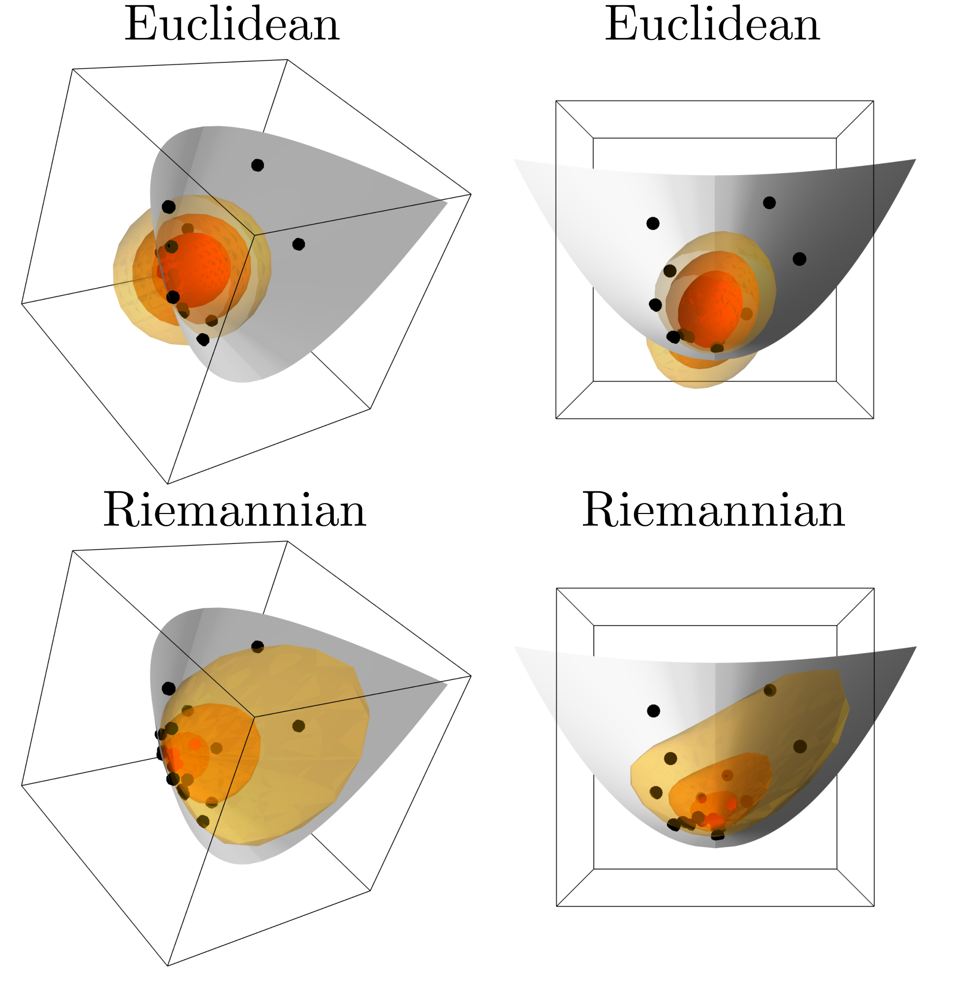
Euclidean probabilistic models on manifold data assign probability mass to impossible data points under spatial constraints. Furthermore, points that are similar under the chosen non-Euclidean metric can be assigned very different likelihoods, which can cause a poor fit to the data. Both issues affect especially the uncertainty estimates. These issues can be avoided by exploiting the Riemannian geometry in the model. Fig. 1 shows points in , the space of symmetric positive-definite matrices, with fitted Euclidean and Riemannian models. The points outside the cone are not matrices. Under the Log-Euclidean metric, which generalizes the log transform to matrices, elements on the boundary (in gray) lie infinitely far from interior points. The metrics, and hence the induced models, are vastly different. This results in the Riemannian model with an improved model fit.
Contributions. Motivated by these observations, we introduce the wrapped Gaussian process latent variable model (WGPLVM). This extends the Gaussian process latent variable model (GPLVM) to data on Riemannian manifolds by employing wrapped Gaussian processes (WGPs). Like the GPLVM, the WGPLVM defines a probabilistic model between elements in a lower dimensional latent space and the data, providing uncertainty estimates. As WGPs take values strictly on a given Riemannian manifold, the WGPLVM enforces known constraints and invariances, and accounts for modelling choices concerning the metric.
We demonstrate the WGPLVM on several different manifolds and tasks. We show that our method provides more efficient encoding of the original data compared to the Euclidean GPLVM, provides superior uncertainty estimates and better captures trends in the data, resulting in improved visualization results.
Related Literature. First, we discuss methods in manifold learning, which view data points as elements of a Euclidean space. Then, we discuss related work in submanifold learning, that works strictly on Riemannian manifolds. Note that some manifold learning methods can impose known geometry on the latent space. Models relying on kernels (e.g. the GPLVM and WGPLVM) can encode such structure on the latent space (Lin et al., 2017). This is different from imposing geometric constraints on the data space.
Manifold learning infers a low-dimensional manifold that captures the trend of given data. Classical algorithms (Tenenbaum et al., 2000; Roweis and Saul, 2000; Belkin and Niyogi, 2003) learn a low distortion projection from a data submanifold of the original, Euclidean ambient space, onto a low-dimensional Euclidean space. Latent variable models (LVMs) (Kingma and Welling, 2014; Goodfellow et al., 2014; Lawrence, 2005) learn the reverse latent embedding from the latent space into the ambient space, associating each point in the latent space with an ambient space point. In the well-known Gaussian process latent variable model (GPLVM) (Lawrence, 2005), the latent embedding is a Gaussian process (GP) over the latent space, and hence learns not only a manifold embedding into , but also a model of its uncertainty. GPLVMs have inspired other LVMs (Titsias and Lawrence, 2010; Lawrence and Moore, 2007; Urtasun and Darrell, 2007), that all rely on Euclidean geometry. Urtasun et al. (2008) consider topologically constrained LVMs and Varol et al. (2012) consider GPLVMs with spatial constraints, where the constraints are enforced through slack variables and local linearization. Our method works intrinsically on the specific Riemannian manifold, taking the topology, spatial constraints and the Riemannian metric into account. Thus the WGPLVM falls into the category of submanifold learning.
Submanifold learning algorithms, illustrated in Fig. 2, aim to infer a model from a latent space to a submanifold (dashed red) of a known ambient manifold of points that satisfy the constraints. The map associates the data (dark grey) with latent variables (blue). Principal geodesic analysis (PGA) (Fletcher et al., 2004; Huckemann et al., 2010) estimates geodesic submanifolds, Riemannian principal curves (Hauberg, 2016) and barycentric subspaces (Pennec, 2015) estimate less constrained submanifolds. Probabilistic PGA (Zhang and Fletcher, 2013) introduces uncertainty by estimating probabilistic geodesic subspaces. The WGPLVM contributes non-geodesic, probabilistic learning of the submanifold from a prior model, allowing considerable flexibility compared to previous models.
Examples of manifold valued data include directional statistics, which consider spherical data (Urtasun et al., 2006; Mardia and Jupp, 2009), covariance matrices as data objects in economics and computer vision (Wilson and Ghahramani, 2011; Tuzel et al., 2006) and in diffusion MRI or materials science (Batchelor et al., 2005; Fletcher and Joshi, 2004), and statistics of shape, which is of fundamental interest in computer vision (Kendall, 1984; Freifeld and Black, 2012). In each example, the common approach is to incorporate the Riemannian structure in the statistical analysis.
2 PRELIMINARIES
This section introduces the necessary preliminaries and notation. We first review Gaussian processes (GPs) and the Gaussian process latent variable model (GPLVM) (Lawrence, 2004). Next, we summarize the necessary concepts from Riemannian geometry. Subsequently, we review the wrapped Gaussian processes (WGPs) introduced by Mallasto and Feragen (2018), which form the cornerstone of the present work.
Gaussian processes. Let denote a multivariate Gaussian distribution (GD) with mean and covariance matrix , and write the associated probability density function as for . A Gaussian process (GP) is a collection of random variables, so that any finite subcollection is jointly Gaussian, where are elements of the index set. Any GP is uniquely characterized by
| (1) | ||||
called the mean function and covariance function , denoted . For more about GPs and their applications, see Rasmussen (2004).
Gaussian process latent variable model. The Gaussian process latent variable model (GPLVM) is a GP-based dimensionality reduction technique, which aims to learn a probabilistic model relating elements in the low dimensional latent space to observed data , with . The model approximates the manifold that lives on. The probabilistic model is computed by choosing a prior GP with hyper-parameters . The hyper-parameters are optimized with the latent variables to maximize the log-likelihood
| (2) | ||||
where , and denote the corresponding data matrices. Finally, we condition the optimal prior on the chosen latent variables and data , to yield the predictive distribution of the model. Note that any prediction has support in the whole , thus ignoring any constraints or invariances.
In differential geometric terms, a GPLVM can be viewed to learn a stochastic chart for the approximate manifold on which the dataset lives.
Riemannian geometry. A Riemannian manifold is a smooth manifold with a Riemannian metric, i.e. a smoothly varying inner product on the tangent space at each , which induces a distance function on . Each in the tangent bundle defines a geodesic (locally shortest path) on , so that and .
The Riemannian exponential map is given by , where is the geodesic corresponding to . The exponential at is a diffeomorphism between a neighborhood and a neighborhood , which is chosen in a maximal way to preserve injectivity. The logarithmic map is characterized by the identity . Outside of , we use to denote with a minimal norm, chosen in a measurable way. The complement of in is called the cut-locus at , where unique geodesics cannot be defined. Multiple useful manifolds have empty cut-locus, so that , including manifolds with non-positive curvature as well as the space of positive-definite symmetric matrices used below.
Let and . The differential (in some coordinate chart) is given by (see supplementary material for (Pennec, 2016))
| (3) |
where are Jacobi fields solving the linear ordinary differential equation
| (4) |
with initial conditions , , and , . Here is given by and is an orthonormal basis for , defined by and each evolves through parallel transportation. Furthermore, denotes the curvature tensor and is the -by- identity matrix, where is the dimension of the manifold. For a thorough exposition in Riemannian geometry, see (Do Carmo, 1992).
Let be Riemannian manifolds with metrics , exponential maps and logarithmic maps for . Then turns into a Riemannian manifold when endowed with the metric , which has the component-wise computed exponential map . The logarithmic map on the product manifold is defined likewise.

Wrapped Gaussian distributions. Let be an -dimensional geodesically complete Riemannian manifold. Let be a measure on and be a measurable map. We define the push-forward as for any measurable set in . A random point on follows a wrapped Gaussian distribution (WGD), if for some and a symmetric positive definite matrix
| (5) |
denoted by . The WGD is thus defined by a GD in the tangent space , that is pushed-forward onto by the exponential map (see Fig. 3). We call the basepoint of , and the tangent space covariance.
Two random points , are jointly WGD, if is a WGD on the product manifold , given by
| (6) |
for some matrix . Then, can be conditioned on , resulting in a push-forward of a Gaussian mixture in by the exponential map
| (7) |
where is the preimage of . The means and covariance matrices of the Gaussian mixture components are given by
| (8) |
and the component weights are
| (9) |
Wrapped Gaussian processes.
Wrapped Gaussian processes generalize GPs to Riemannian manifolds (Mallasto and Feragen, 2018). A collection of random points on a Riemannian manifold indexed over a set is a wrapped Gaussian process (WGP), if every finite subcollection is jointly WGD on . The functions
| (10) | ||||
are called the basepoint function and the tangent space covariance function of (also called as kernel of ), respectively. To denote such a WGP, we use the notation .
Formally, a WGP can be viewed as a GP on , the family of tangent spaces over the basepoint function . Then, the resulting GP is pushed forward to using the Riemannian exponential map over to obtain the WGP, see Fig. 4.

3 WRAPPED GAUSSIAN PROCESS LATENT VARIABLE MODEL
We now introduce the wrapped Gaussian process latent variable model (WGPLVM) for data lying on an -dimensional ambient Riemannian manifold . The goal of WGPLVM is to learn a lower-dimensional submanifold , where the data is assumed to reside. The WGPLVM model is a straight-forward generalization of the GPLVM model, where instead of GPs, we maximize the likelihood of our data combined with the latent variables under the WGPs that are suitable for the manifold context. The WGPLVM pipeline is illustrated in Fig. 5.
We consider a family of WGPs from the latent space onto the ambient manifold , where are hyperparameters, that will be optimized over. The basepoint function can be utilized to delocalize the learning process in order to avoid distortions of the metric caused by linearization of the curved . The kernel affects how observations in different tangent spaces affect each other. For coherence, the kernel should be adapted to a smooth frame (a smoothly changing basis over ). Such a frame can e.g. be constructed by parallel transporting a basis along .
The likelihood assigned by the prior to a data point with associated latent variable is
| (11) | ||||
where and .
The approximation in Eq. (11) only takes into account the preimage of with a minimal norm (and thus maximal likelihood), denoted by . The expression gives a lower bound for , thus, maximizing the likelihood of maximizes the lower bound for . It also enforces the WGPLVM to prefer local models over ones that wrap considerably around the manifold. Note that, for manifolds with empty cut-locus (such as ones with non-positive curvature), the approximation in (11) is exact.
The objective function to be maximized is then the approximated log-likelihood
| (12) | ||||
for which the gradient with respect to is given by
| (13) | ||||
The differential can be computed using Jacobi fields as explained in expression (3), if no analytical expression exists.
Assuming that the data is i.i.d, the approximate log-likelihood for the data set can be written using Eq. (12), by considering as a single element of the product manifold . This quantitity is then maximized by optimizing over the latent variables and the hyperparameters , resulting in the optimal latent variables and hyperparameters for the kernel.
The approximate submanifold can then be predicted at arbitrary latent variables , by conditioning on the data with the associated latent variables (using Eq. (7)). The conditional distribution will then be a non-centered GP defined on pushed forward by the exponential map (see Fig. 5), resulting in the predictive distribution . Then, the mean prediction is given by .
In Eq. (7), if the preimage is not uniquely defined, the conditional distribution is approximated by using a preimage with minimal norm, as previously. This approximation is justified as the weights of the components of the Gaussian mixture decrease exponentially as increases.
The initial latent variables can be chosen strategically to aid optimization. We use principal geodesic analysis (PGA) (Fletcher et al., 2004) and principal curves (Hauberg, 2016). PGA is appropriate when the data expresses a geodesic trend (analogy of linearity on Riemannian manifolds), which is not the case for the femur dataset, see Fig. 6 in Section 4.
The Computational complexity for the method is , where is the cost of computing the Riemannian logarithm. This varies from manifold to manifold, but for example, in Section 4, the most expensive is for the Log-Euclidean metric on symmetric, positive-definite matrices.
We provide a pseudo-algorithm for the method in the supplementary material.
4 EXPERIMENTS
The WGPLVM is demonstrated on three different manifolds, arising from three different applications: The sphere, Kendall’s shape space (Kendall, 1984), and the space of symmetric, positive definite (SPD) matrices. Furthermore, the WGPLVM is compared with the Euclidean GPLVM, whose predictive distribution is expected not to lie on the manifold. This effect is clearly visible in Fig. 6. A third model, also shown in Fig. 6, is a modification of the Euclidean GPLVM, where the GP predictions are projected onto the manifold in order to make them satisfy the desired constraints.
We first introduce the datasets and their associated tasks, along with dataset-specific details related to training the models. In each case, we train the model assuming independent coordinates, applying the same kernel to each coordinate.
Femur dataset on . A set of directions of the left femur bone of a person walking in a circular pattern (CMU Graphics Lab, 2003; Hauberg, 2016) is measured at time points. The movement is expected to be one dimensional and periodic, and thus we learn a -dimensional submanifold homeomorphic to a circle to approximate the data manifold. The latent variable optimization is initialized using principal curves (Hauberg, 2016), and the prior WGP and GP had kernel
| (14) |
and mean and , respectively, where is the Fréchet mean of the training set and are hyperparameters optimized to maximize the likelihood of the dataset with the latent variables . The trained models are visualized in Fig. 6.
Diatom shapes in Kendall’s shape space. Diatoms are unicellular algae, whose species are related to their shapes. In Kendall’s shape space we analyze a set of outline shapes of 780 diatoms (Jalba et al., 2006; du Buf and Bayer, 2002) from 37 different species. For visualization, a two dimensional latent space is learned, using the prior , with constant basepoint function set to be the Fréchet mean of the population and given by the radial basis function (RBF) kernel
| (15) |
We initialize the GPLVM and WGPLVM models with PGA and PCA, respectively.
Diffusion tensors in . In the space of SPD matrices with the Log-Euclidean metric (Arsigny et al., 2006), we collect a set of diffusion tensors from a diffusion MRI dataset, sampled with approximately uniform fractional anisotropy (FA) values. The FA is a well-known tensor shape descriptor; see the supplementary material for the definition. As SPD matrices form an open subset of the Euclidean space of symmetric matrices, we do not get a “for free” dimensionality reduction by restricting to SPD matrices. Instead, the data is transformed nonlinearly according to the Log-Euclidean metric, which is commonly used for diffusion tensors (Arsigny et al., 2006). The diffusion MRI image was a single subject from the Human Connectome Project (Van Essen et al., 2013; Glasser et al., 2013; Sotiropoulos et al., 2013). In diffusion MRI, low-dimensional encoding with uncertainty estimates may speed up image acquisition and processing.
| Riemannian | Femur | Diatoms | Diffusion tensors | Crypto-tensors |
|---|---|---|---|---|
| GPLVMProj | ||||
| WGPLVM |
| Euclidean | Femur | Diatoms | Diffusion tensors | Crypto-tensors |
|---|---|---|---|---|
| GPLVM | ||||
| GPLVMProj | ||||
| WGPLVM |
Crypto-tensors in . On we collect the price of 10 popular crypto-currencies11 1 Bitcoin, Dash, Digibyte, Dogecoin, Litecoin, Vertcoin, Stellar, Monero, Ripple, and Verge. in the time 2.12.2014-15.5.2018. The crypto-currency intra-relationship at a given time is encoded in the covariance matrix between the prices in the past 20 days; we include every th day in the period, resulting in covariance matrices. Wilson and Ghahramani (2011) provide a discussion of covariance descriptors in economy. As the acquired covariance matrices in have eigenvalues in different orders of magnitude, we use the Log-Euclidean metric (Arsigny et al., 2006), capturing this trend better.
For both datasets, the basepoint function, the kernel and the latent variable initialization are chosen as for Kendall’s shape space. The latent spaces are chosen to be -dimensional for visualization purposes.
Application 1: Encoding. The datasets are divided into training and test sets (consisting of and of the data, respectively), and we learn the models on the training set. Each test element is “encoded” by the projection . We assess the quality of this encoding by measuring the root-mean-square error (RMSE) of the reconstruction, where the error is measured both by the Euclidean metric and the intrinsic metric. Each experiment was repeated 10 times with different training and test sets; the results are reported in Table 1.
Under the intrinsic metric, the WGPLVM performs significantly better on the tensor datasets, and marginally better in the two other cases. Under the Euclidean metric the WGPLVM encoding is better in two cases, worse in one, and inconclusive for the crypto-tensors where no model is significantly better than the others.


Application 2: Uncertainty quantification. Importantly, GPLVM learns a probabilistic model, producing an estimate of uncertainty. We evaluate these uncertainty estimates on all four datasets. Since the predictive distributions live in different spaces, the likelihoods of observed data under the different models are not directly comparable. However, all three models yield confidence intervals, which we compare using 10 resampled training and test sets ( and of the data). The test set is projected onto the predicted submanifold via . Then, we sample the respective predictive distributions times, computing the fraction of samples closer to the mean prediction than the test point. The results are visualized in Fig. 8, where the densities of these fractions are shown with corresponding cumulative distributions. For a perfect model fit, we would observe the curve (dashed line) as the cumulative distribution. The experiment shows that all models estimate uncertainty incorrectly, but that WGPLVM obtains the best estimate.
Application 3: Visualization. In Fig. 7, we illustrate the latent spaces of WGPLVM versus GPLVM on the crypto-tensor dataset, which comes with an associated time variable, shown in color. The WGPLVM provides a smoother and more consistent transition in color, while the GPLVM plots all the earlier (dark blue) tensors on top of each other. Similar visualizations for the other datasets can be found in the supplementary material; in these examples, the two visualizations are not significantly different in quality.
In the supplementary material, we provide a discussion on why our model might perform better in the experiments, including a comparison between the Euclidean and Riemannian geometries.
5 DISCUSSION AND CONCLUSION
We introduced the WGPLVM for non-parametric and probabilistic submanifold learning on Riemannian manifolds. The model encodes known constraints or invariances, and provides model flexibility, as metrics other than the Euclidean one can be incorporated. This is useful if a different metric captures trends in the data better. The model was evaluated on several manifolds and tasks against the GPLVM and a modified GPLVM, which projects predictions onto the manifold.
The experimental results show that the WGPLVM provides a better probabilistic model to fit the data; in particular the uncertainty estimates are superior to the Euclidean models on three out of four datasets, and virtually identical on the fourth. We note that for Euclidean models, the uncertainty is visibly higher. These are strong indications that our model carries out modelling the data distribution better. The mean predictions of the WGPLVM encode the data space significantly better than the GPLVM and projected GPLVM models on two of the datasets, and marginally better on the other two, when measured in the Riemannian metric. Under the Euclidean metricr, the GPVLM performs notably better in one experiment, and WGPLVM marginally better in two. On crypto-tensors, we deem the results inconclusive due to high variance. The aforementioned effects are also seen in the latent space visualizations, e.g. on the cryptotensors the WGPLVM better detects small-scale differences in the early time steps.
One might suspect that the improved performance stems from a “for free” dimensionality reduction through constraints. However, we note that the most significant improvement in both reconstruction error and visualization was obtained on , where the Riemannian manifold is a full-dimensional, convex subset of the Euclidean ambient space. This might still be due to the constraints, which forces the distributions to lie in the manifold. The difference could also be caused by the choice of metric. For the crypto-tensors in particular, we observe that some of the eigenvalues are very small; the Log-Euclidean metric essentially acts as a log-transform and therefore converts the data to a scale on which changes in the smaller eigenvalues can be detected.
In three of the experiments, the mean predictions of GPLVM lie essentially on the manifold, thus the projected version does not improve the mean reconstruction error. However, in the femur experiment, the uncertainty estimates are clearly improved, but also notably outperformed by WGPLVM. Due to the metric and curvature of the manifold, interpolation between two points in the ambient space does not necessarily project even closely onto the manifold interpolation between the projected points. This distortion affects the statistics relying on interpolation, and explains both the reduced reconstruction capability and the increased variance. Furthermore, the projected model ignores any metric choices imposed on the manifold.
Although the WGPLVM provides flexibility through the prior basepoint function, we fixed this to be the Fréchet mean of the training set in our experiments. The choice is well justified if the data is local enough, and makes the comparison to GPLVM fair. The flexibility to delocalize the learning process through the basepoint function is, however, important for inference on manifolds when the locality assumption fails. The non-trivial optimization of the basepoint function thus provides a venue for future research.
In summary, the WGPLVM is a probabilistic submanifold learning algorithm that respects known Riemannian manifold structure in the data by taking values in the associated Riemannian manifold. We compare the model to its Euclidean counterparts on a number of manifolds, datasets and tasks, and show that it has superior representation capabilities more faithful visualizations and improved uncertainty estimates.
Acknowledgements
AM and AF were supported by Centre for Stochastic Geometry and Advanced Bioimaging, funded by a grant from the Villum Foundation, and SH was supported by the European Research Council (ERC) under the European Union’s Horizon 2020 research and innovation programme (grant agreement n∘ 757360), as well as a research grant (15334) from VILLUM FONDEN. Data were provided [in part] by the Human Connectome Project, WU-Minn Consortium (Principal Investigators: David Van Essen and Kamil Ugurbil; 1U54MH091657) funded by the 16 NIH Institutes and Centers that support the NIH Blueprint for Neuroscience Research; and by the McDonnell Center for Systems Neuroscience at Washington University. The data [in part] used in this project was obtained from mocap.cs.cmu.edu. The database was created with funding from NSF EIA-0196217. The authors wish to thank Thomas Hamelryck for helpful comments.
References
- Arsigny et al. (2006) Vincent Arsigny, Pierre Fillard, Xavier Pennec, and Nicholas Ayache. Log-euclidean metrics for fast and simple calculus on diffusion tensors. Magnetic Resonance in Medicine: An Official Journal of the International Society for Magnetic Resonance in Medicine, 56(2):411–421, 2006.
- Batchelor et al. (2005) Phillipp G. Batchelor, Maher Moakher, David. Atkinson, Fernando. Calamante, and Alan Connelly. A rigorous framework for diffusion tensor calculus. Magnetic Resonance in Medicine, 53(1):221–225, 2005. ISSN 1522-2594.
- Belkin and Niyogi (2003) Mikhail Belkin and Partha Niyogi. Laplacian eigenmaps for dimensionality reduction and data representation. Neural Computation, 15(6):1373–1396, 2003.
- CMU Graphics Lab (2003) CMU Graphics Lab. CMU Graphics Lab Motion Capture Database . http://mocap.cs.cmu.edu/, 2003. The data used in this project was obtained from mocap.cs.cmu.edu. The database was created with funding from NSF EIA-0196217.
- Do Carmo (1992) Manfredo Perdigao Do Carmo. Riemannian geometry. Birkhauser, 1992.
- du Buf and Bayer (2002) Hans du Buf and Micha Bayer. Automatic Diatom Identification. 2002.
- Fletcher and Joshi (2004) P. Thomas Fletcher and Sarang Joshi. Principal Geodesic Analysis on Symmetric Spaces: Statistics of Diffusion Tensors, pages 87–98. 2004.
- Fletcher et al. (2004) P. Thomas Fletcher, Conglin Lu, Stephen M. Pizer, and Sarang Joshi. Principal geodesic analysis for the study of nonlinear statistics of shape. IEEE transactions on medical imaging, 23(8):995–1005, 2004.
- Freifeld and Black (2012) Oren Freifeld and Michael J Black. Lie bodies: A manifold representation of 3D human shape. In A. Fitzgibbon et al. (Eds.), editor, European Conference on Computer Vision (ECCV), Part I, LNCS 7572, pages 1–14. Springer-Verlag, 2012.
- Glasser et al. (2013) Matthew F. Glasser, Stamatios N. Sotiropoulos, J. Anthony Wilson, Timothy S. Coalson, Bruce Fischl, Jesper L. Andersson, Junqian Xu, Saad Jbabdi, Matthew Webster, Jonathan R. Polimeni, et al. The minimal preprocessing pipelines for the Human Connectome project. Neuroimage, 80:105–124, 2013.
- Goodfellow et al. (2014) Ian Goodfellow, Jean Pouget-Abadie, Mehdi Mirza, Bing Xu, David Warde-Farley, Sherjil Ozair, Aaron Courville, and Yoshua Bengio. Generative adversarial nets. In Advances in Neural Information Processing Systems (NIPS), 2014.
- Hauberg (2016) Søren Hauberg. Principal curves on Riemannian manifolds. IEEE Transactions on Pattern Analysis and Machine Intelligence (TPAMI), 2016.
- Hauberg et al. (2012) Søren Hauberg, Oren Freifeld, and Michael J. Black. A geometric take on metric learning. In P. Bartlett, F.C.N. Pereira, C.J.C. Burges, L. Bottou, and K.Q. Weinberger, editors, Advances in Neural Information Processing Systems (NIPS) 25, pages 2033–2041. MIT Press, 2012.
- Huckemann et al. (2010) Stephan Huckemann, Thomas Hotz, and Axel Munk. Intrinsic shape analysis: Geodesic PCA for Riemannian manifolds modulo isometric Lie group actions. Statistica Sinica, pages 1–58, 2010.
- Jalba et al. (2006) Andrei C. Jalba, Michael HF Wilkinson, and Jos BTM Roerdink. Shape representation and recognition through morphological curvature scale spaces. IEEE Transactions on Image Processing, 15(2):331–341, feb 2006.
- Kendall (1984) David G. Kendall. Shape manifolds, Procrustean metrics, and complex projective spaces. Bulletin of the London Mathematical Society, 16(2):81–121, 1984.
- Kingma and Welling (2014) Diederik P. Kingma and Max Welling. Auto-Encoding Variational Bayes. In Proceedings of the 2nd International Conference on Learning Representations (ICLR), 2014.
- Lawrence (2004) Neil D Lawrence. Gaussian process latent variable models for visualisation of high dimensional data. In Advances in neural information processing systems, pages 329–336, 2004.
- Lawrence (2005) Neil D. Lawrence. Probabilistic non-linear principal component analysis with Gaussian process latent variable models. J. Mach. Learn. Res., 6:1783–1816, 2005. ISSN 1532-4435.
- Lawrence and Moore (2007) Neil D. Lawrence and Andrew J. Moore. Hierarchical Gaussian process latent variable models. In Proceedings of the 24th international conference on Machine learning, pages 481–488. ACM, 2007.
- Lin et al. (2017) Lizhen Lin, Mu Niu, Pokman Cheung, and David Dunson. Extrinsic gaussian processes for regression and classification on manifolds. arXiv preprint arXiv:1706.08757, 2017.
- Mallasto and Feragen (2018) Anton Mallasto and Aasa Feragen. Wrapped Gaussian process regression on Riemannian manifolds. In CVPR - IEEE Conference on Computer Vision and Pattern Recognition, to appear, 2018.
- Mardia and Jupp (2009) Kanti V. Mardia and Peter E. Jupp. Directional statistics, volume 494. John Wiley & Sons, 2009.
- Pennec (2015) Xavier Pennec. Barycentric subspaces and affine spans in manifolds. In Geometric Science of Information - Second International Conference, GSI 2015, Palaiseau, France, October 28-30, 2015, Proceedings, pages 12–21, 2015.
- Pennec (2016) Xavier Pennec. Barycentric subspace analysis on manifolds. arXiv preprint arXiv:1607.02833, 2016.
- Rasmussen (2004) Carl Edward Rasmussen. Gaussian processes in machine learning. In Advanced lectures on machine learning, pages 63–71. Springer, 2004.
- Roweis and Saul (2000) Sam T. Roweis and Lawrence K. Saul. Nonlinear dimensionality reduction by locally linear embedding. SCIENCE, 290:2323–2326, 2000.
- Sotiropoulos et al. (2013) Stamatios N. Sotiropoulos, Steen Moeller, Saad Jbabdi, Jungqian Xu, Jesper Andersson, Edward John Auerbach, Essa Yacoub, David A. Feinberg, Kawin Setsompop, Lawrence L. Wald, et al. Effects of image reconstruction on fiber orientation mapping from multichannel diffusion MRI: reducing the noise floor using SENSE. Magnetic resonance in medicine, 70(6):1682–1689, 2013.
- Tenenbaum et al. (2000) Joshua B. Tenenbaum, Vin de Silva, and John C. Langford. A global geometric framework for nonlinear dimensionality reduction. Science, 290(5500):2319–2323, 2000.
- Titsias and Lawrence (2010) Michalis Titsias and Neil D. Lawrence. Bayesian Gaussian process latent variable model. In Proceedings of the Thirteenth International Conference on Artificial Intelligence and Statistics, pages 844–851, 2010.
- Tuzel et al. (2006) Oncel. Tuzel, Fatih Porikli, and Peter Meer. Region covariance: A fast descriptor for detection and classification. European Conference on Computer Vision (ECCV), pages 589–600, 2006.
- Urtasun and Darrell (2007) Raquel Urtasun and Trevor Darrell. Discriminative Gaussian process latent variable model for classification. In Proceedings of the 24th international conference on Machine learning, pages 927–934. ACM, 2007.
- Urtasun et al. (2006) Raquel Urtasun, David J. Fleet, and Pascal Fua. 3d people tracking with Gaussian process dynamical models. In Computer Vision and Pattern Recognition, 2006 IEEE Computer Society Conference on, volume 1, pages 238–245. IEEE, 2006.
- Urtasun et al. (2008) Raquel Urtasun, David J. Fleet, Andreas Geiger, Jovan Popović, Trevor J. Darrell, and Neil D Lawrence. Topologically-constrained latent variable models. In Proceedings of the 25th international conference on Machine learning, pages 1080–1087. ACM, 2008.
- Van Essen et al. (2013) David C. Van Essen, Stephen M. Smith, Deanna M. Barch, Timothy EJ Behrens, Essa Yacoub, Kamil Ugurbil, Wu-Minn HCP Consortium, et al. The wu-minn Human Connectome project: an overview. Neuroimage, 80:62–79, 2013.
- Varol et al. (2012) Aydin Varol, Mathieu Salzmann, Pascal Fua, and Raquel Urtasun. A constrained latent variable model. In Computer Vision and Pattern Recognition (CVPR), 2012 IEEE Conference on, pages 2248–2255. Ieee, 2012.
- Wilson and Ghahramani (2011) Andrew Gordon Wilson and Zoubin Ghahramani. Generalised Wishart processes. In UAI 2011, Proceedings of the Twenty-Seventh Conference on Uncertainty in Artificial Intelligence, Barcelona, Spain, July 14-17, 2011, pages 736–744, 2011.
- Zhang and Fletcher (2013) Miaomiao Zhang and P. Thomas Fletcher. Probabilistic principal geodesic analysis. In Advances in Neural Information Processing Systems 26: 27th Annual Conference on Neural Information Processing Systems 2013. Proceedings of a meeting held December 5-8, 2013, Lake Tahoe, Nevada, United States., pages 1178–1186, 2013.
Supplementary Material
A Pseudo-Algorithm forWGPLVM
A pseudo-code algorithm for training the WGPLVM is provied in Alg. 1.
B Details on Manifolds Used
The -sphere is a Riemannian manifold with exponential and logarithmic maps given by
| (16) |
where is the -norm induced by the standard Euclidean innerproduct .
Kendall’s shape space forms a quontient manifold of the sphere, so the operations defined for apply, when working with the right quotient representatives. Kendall’s shape space has the additional constraint of representing shapes with respect to an optimal translation between a pair of shapes. Let be the data matrices of two shapes, where is the amount of landmarks, and each column represents the -coordinates after quontienting away scale and translation. Then, the Procrustean distance between the shapes is given by
| (17) |
where is a rotation matrix. The shapes are aligned by choosing a reference point, and aligning the population elements by minimizing the Procrustean distance.
The space of symmetric, positive definite matrices can be given the structure of a Riemannian manifold, by endowing it with the Log-Euclidean metric. The tangent space at each point is the space of -by- symmetric matrices, and the affine-invariant metric is given by
| (18) |
and the exponential and logarithmic maps are given by
| (19) |
where stands for the matrix exponential and for the matrix logarithm.
C Latent Space Visualization
Here we provide the latent space visualizations for the diffusion-tensor and diatom datasets.


The fractional anisotropy (FA) of a SPD matrix is a shape descriptor taking values between and , where an FA of corresponds to a round tensor, and an FA near corresponds to a very thin one. Given the eigenvalues for an SPD matrix, its FA is defined as
where is the mean of the eigenvalues. In the latent space shown in Fig. 9, the latent variables are colored according to the FA of their associated tensor, and we see that both models provide a smooth transition between different FA values.
The latent space visualization of the diatom dataset is found in Fig. 10; here the latent variables are colored by the species of the corresponding diatom, see Fig. 11 for a visualization of species representatives.


D Comparing the Geometries
In this section, we compare the geometries in Euclidean and Riemannian cases. The aim is to try and understand, when the performance is improved. We do this by visualizing the distribution of data point distances to the corresponding population means, the distances and means computed according to the corresponding metrics.
As can be seen in Fig. 12, in the femur (-sphere) and diatom (Kendall’s shape space) cases, the distributions look very similar. In fact, in the diatom case, they are essentially the same. The Kendall’s shape space forms a quotient manifold of the sphere, which in this case is high dimensional (). In such high dimension, escaping the manifold becomes increasingly more difficult (most of the volume of the sphere is close to the boundary), and thus both the metrics are essentially the same. This might explain, why the WGPLVM did not improve notably on the GPLVM.
In the crypto-tensor experiment, the distribution implies the presence of extreme outliers under the Euclidean metric. The Log-Euclidean metric, on the other hand, transforms the metric scale, evening out the distribution. This could very well explain, why we see large improvement with the WGPLVM compared to the GPLVM.
In the DTI experiment, the distribution of Euclidean distances looks more even. This might imply, that in this occasion, the Euclidean distance is better at capturing the trend of the data. However, the improved uncertainty estimates of the WGPLVM could be explained, as the Euclidean models are not confined to . Therefore, the distributions do not follow the conic shape of .