Hyperbolic Neural Networks

The Möbius addition of $x$ and $y$ in ${\mathbb{D}}_{c}^{n}$ is defined as

In particular, when $c=0$, one recovers the Euclidean addition of two vectors in ${\mathbb{R}}^{n}$. Note that without loss of generality, the case $c>0$ can be reduced to $c=1$. Unless stated otherwise, we will use $\oplus$ as $\oplus_{1}$ to simplify notations. For general $c>0$, this operation is not commutative nor associative. However, it satisfies $x\oplus_{c}\textbf{0}=\textbf{0}\oplus_{c}x=\textbf{0}$. Moreover, for any $x,y\in{\mathbb{D}}^{n}_{c}$, we have $(-x)\oplus_{c}x=x\oplus_{c}(-x)=\textbf{0}$ and $(-x)\oplus_{c}(x\oplus_{c}y)=y$ (left-cancellation law). The Möbius substraction is then defined by the use of the following notation: $x\ominus_{c}y:=x\oplus_{c}(-y)$. See (29, section 2.1) for a geometric interpretation of the Möbius addition.

For $c>0$, the Möbius scalar multiplication of $x\in{\mathbb{D}}_{c}^{n}\setminus\{\textbf{0}\}$ by $r\in\mathbb{R}$ is defined as

and $r\otimes_{c}\textbf{0}:=\textbf{0}$. Note that similarly as for the Möbius addition, one recovers the Euclidean scalar multiplication when $c$ goes to zero: $\lim_{c\to 0}r\otimes_{c}x=rx$. This operation satisfies desirable properties such as $n\otimes_{c}x=x\oplus_{c}\dots\oplus_{c}x$ ($n$ additions), $(r+r^{\prime})\otimes_{c}x=r\otimes_{c}x\oplus_{c}r^{\prime}\otimes_{c}x$ (scalar distributivity²² 2 $\otimes_{c}$ has priority over $\oplus_{c}$ in the sense that $a\otimes_{c}b\oplus_{c}c:=(a\otimes_{c}b)\oplus_{c}c$ and $a\oplus_{c}b\otimes_{c}c:=a\oplus_{c}(b\otimes_{c}c)$.), $(rr^{\prime})\otimes_{c}x=r\otimes_{c}(r^{\prime}\otimes_{c}x)$ (scalar associativity) and $|r|\otimes_{c}x/\|r\otimes_{c}x\|=x/\|x\|$ (scaling property).

If one defines the generalized hyperbolic metric tensor $g^{c}$ as the metric conformal to the Euclidean one, with conformal factor $\lambda_{x}^{c}:=2/(1-c\|x\|^{2})$, then the induced distance function on $({\mathbb{D}}_{c}^{n},g^{c})$ is given by³³ 3 The notation $-x\oplus_{c}y$ should always be read as $(-x)\oplus_{c}y$ and not $-(x\oplus_{c}y)$.

Again, observe that $\lim_{c\to 0}d_{c}(x,y)=2\|x-y\|$, i.e. we recover Euclidean geometry in the limit⁴⁴ 4 The factor $2$ comes from the conformal factor $\lambda_{x}=2/(1-\|x\|^{2})$, which is a convention setting the curvature to $-1$.. Moreover, for $c=1$ we recover $d_{\mathbb{D}}$ of Eq. (4).

Similarly as in the Euclidean space, one can define the notions of hyperbolic angles or gyroangles (when using the $\oplus_{c}$), as well as hyperbolic law of sines in the generalized Poincaré ball $({\mathbb{D}}_{c}^{n},g^{c})$. We make use of these notions in our proofs. See Appendix A.

The Riemannian gyroline element is defined for an infinitesimal $dx$ as $ds:=(x+dx)\ominus_{c}x$, and its size is given by (26, section 3.7):

What is remarkable is that it turns out to be identical, up to a scaling factor of $2$, to the usual line element $2\|dx\|/(1-c\|x\|^{2})$ of the Riemannian manifold $({\mathbb{D}}_{c}^{n},g^{c})$.

The geodesic connecting points $x,y\in{\mathbb{D}}_{c}^{n}$ is shown in (2, 26) to be given by:

Note that when $c$ goes to $0$, geodesics become straight-lines, recovering Euclidean geometry. In the remainder of this subsection, we connect the gyrospace framework with Riemannian geometry.

The following lemma gives the closed-form derivation of exponential and logarithmic maps.

The above maps have more appealing forms when $x=\textbf{0}$, namely for $v\in T_{\textbf{0}}{\mathbb{D}}^{n}_{c}\setminus\{\textbf{0}\},\ y\in{\mathbb{D}}^{n}_{c}\setminus\{\textbf{0}\}$:

Moreover, we still recover Euclidean geometry in the limit $c\to 0$, as $\lim_{c\to 0}\exp_{x}^{c}(v)=x+v$ is the Euclidean exponential map, and $\lim_{c\to 0}\log_{x}^{c}(y)=y-x$ is the Euclidean logarithmic map.

We studied the exponential and logarithmic maps in order to gain a better understanding of the Möbius scalar multiplication (Eq. (7)). We found the following:

This last result enables us to generalize scalar multiplication in order to define matrix-vector multiplication between Poincaré balls, one of the essential building blocks of hyperbolic neural networks.

Finally, we connect parallel transport (from $T_{\textbf{0}}{\mathbb{D}}_{c}^{n}$) to gyrovector spaces with the following theorem, which we prove in appendix B.

As we’ll see later, this result is crucial in order to define and optimize parameters shared between different tangent spaces, such as biases in hyperbolic neural layers or parameters of hyperbolic MLR.

Let’s first reformulate Euclidean MLR from the perspective of distances to margin hyperplanes, as in (19, Section 5). This will allow us to easily generalize it.

Given $K$ classes, one learns a margin hyperplane for each such class using softmax probabilities:

Note that any affine hyperplane in ${\mathbb{R}}^{n}$ can be written with a normal vector $a$ and a scalar shift $b$:

As in (19, Section 5), we note that $\langle a,x\rangle-b=\text{sign}(\langle a,x\rangle-b)\|a\|d(x,H_{a,b})$. Using Eq. (17):

As it is not immediately obvious how to generalize the Euclidean hyperplane of Eq. (18) to other spaces such as the Poincaré ball, we reformulate it as follows:

This new definition relates to the previous one as $\tilde{H}_{a,p}=H_{a,\langle a,p\rangle}$. Rewriting Eq. (19) with $b=\langle a,p\rangle$:

It is now natural to adapt the previous definition to the hyperbolic setting by replacing $+$ by $\oplus_{c}$:

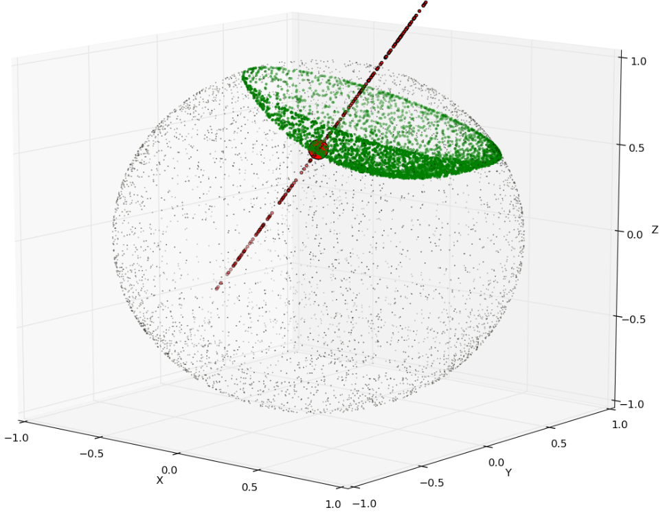
The last equality is shown appendix C. $\tilde{H}_{a,p}^{c}$ can also be described as the union of images of all geodesics in ${\mathbb{D}}^{n}_{c}$ orthogonal to $a$ and containing $p$. Notice that our definition matches that of hypergyroplanes, see (27, definition 5.8). A 3D hyperplane example is depicted in Fig. 1.

Next, we need the following theorem, proved in appendix D:

Putting together Eq. (21) and Thm. 5, we get the hyperbolic MLR formulation. Given $K$ classes and $k\in\{1,\ldots,K\},\ p_{k}\in{\mathbb{D}}^{n}_{c},\ a_{k}\in T_{p_{k}}{\mathbb{D}}^{n}_{c}\setminus\{\textbf{0}\}$:

or, equivalently

Notice that when $c$ goes to zero, this goes to $p(y=k|x)\propto\exp(4\langle-p_{k}+x,a_{k}\rangle)=\exp((\lambda^{0}_{p_{k}})^{2}\langle-p_{k}+x,a_{k}\rangle)=\exp(\langle-p_{k}+x,a_{k}\rangle_{0})$, recovering the usual Euclidean softmax.

However, at this point it is unclear how to perform optimization over $a_{k}$, since it lives in $T_{p_{k}}{\mathbb{D}}_{c}^{n}$ and hence depends on $p_{k}$. The solution is that one should write $a_{k}=P^{c}_{\textbf{0}\to p_{k}}(a^{\prime}_{k})=(\lambda_{\textbf{0}}^{c}/\lambda_{p_{k}}^{c})a^{\prime}_{k}$, where $a^{\prime}_{k}\in T_{\textbf{0}}{\mathbb{D}}_{c}^{n}={\mathbb{R}}^{n}$, and optimize $a^{\prime}_{k}$ as a Euclidean parameter.

If $\varphi:{\mathbb{R}}^{n}\to{\mathbb{R}}^{n}$ is a pointwise non-linearity, then its Möbius version $\varphi^{\otimes_{c}}$ can be applied to elements of the Poincaré ball.

The generalization of a translation in the Poincaré ball is naturally given by moving along geodesics. But should we use the Möbius sum $x\oplus_{c}b$ with a hyperbolic bias $b$ or the exponential map $\exp_{x}^{c}(b^{\prime})$ with a Euclidean bias $b^{\prime}$? These views are unified with parallel transport (see Thm 4). Möbius translation of a point $x\in{\mathbb{D}}_{c}^{n}$ by a bias $b\in{\mathbb{D}}_{c}^{n}$ is given by

We recover Euclidean translations in the limit $c\to 0$. Note that bias translations play a particular role in this model. Indeed, consider multiple layers of the form $f_{k}(x)=\varphi_{k}(M_{k}x)$, each of which having Möbius version $f_{k}^{\otimes_{c}}(x)=\varphi_{k}^{\otimes_{c}}(M_{k}\otimes_{c}x)$. Then their composition can be re-written $f_{k}^{\otimes_{c}}\circ\dots\circ f_{1}^{\otimes_{c}}=\exp_{\textbf{0}}^{c}\circ f_{k}\circ\dots\circ f_{1}\circ\log_{\textbf{0}}^{c}$. This means that these operations can essentially be performed in Euclidean space. Therefore, it is the interposition between those with the bias translation of Eq. (28) which differentiates this model from its Euclidean counterpart.

If a vector $x\in\mathbb{R}^{n+p}$ is the (vertical) concatenation of two vectors $x_{1}\in{\mathbb{R}}^{n}$, $x_{2}\in{\mathbb{R}}^{p}$, and $M\in\mathcal{M}_{m,n+p}({\mathbb{R}})$ can be written as the (horizontal) concatenation of two matrices $M_{1}\in\mathcal{M}_{m,n}({\mathbb{R}})$ and $M_{2}\in\mathcal{M}_{m,p}({\mathbb{R}})$, then $Mx=M_{1}x_{1}+M_{2}x_{2}$. We generalize this to hyperbolic spaces: if we are given $x_{1}\in{\mathbb{D}}_{c}^{n}$, $x_{2}\in{\mathbb{D}}_{c}^{p}$, $x=(x_{1}\ x_{2})^{T}\in{\mathbb{D}}_{c}^{n}\times{\mathbb{D}}_{c}^{p}$, and $M,M_{1},M_{2}$ as before, then we define $M\otimes_{c}x:=M_{1}\otimes_{c}x_{1}\oplus_{c}M_{2}\otimes_{c}x_{2}$. Note that when $c$ goes to zero, we recover the Euclidean formulation, as $\lim_{c\to 0}M\otimes_{c}x=\lim_{c\to 0}M_{1}\otimes_{c}x_{1}\oplus_{c}M_{2}\otimes_{c}x_{2}=M_{1}x_{1}+M_{2}x_{2}=Mx$. Moreover, hyperbolic vectors $x\in{\mathbb{D}}_{c}^{n}$ can also be "concatenated" with real features $y\in{\mathbb{R}}$ by doing: $M\otimes_{c}x\oplus_{c}y\otimes_{c}b$ with learnable $b\in{\mathbb{D}}_{c}^{m}$ and $M\in\mathcal{M}_{m,n}({\mathbb{R}})$.

A simple RNN can be defined by $h_{t+1}=\varphi(Wh_{t}+Ux_{t}+b)$ where $\varphi$ is a pointwise non-linearity, typically $\tanh$, sigmoid, ReLU, etc. This formula can be naturally generalized to the hyperbolic space as follows. For parameters $W\in\mathcal{M}_{m,n}({\mathbb{R}})$, $U\in\mathcal{M}_{m,d}({\mathbb{R}})$, $b\in{\mathbb{D}}_{c}^{m}$, we define:

Note that if inputs $x_{t}$’s are Euclidean, one can write $\tilde{x}_{t}:=\exp_{0}^{c}(x_{t})$ and use the above formula, since $\exp^{c}_{W\otimes_{c}h_{t}}(P^{c}_{\textbf{0}\to W\otimes_{c}h_{t}}(Ux_{t}))=W\otimes_{c}h_{t}\oplus_{c}\exp^{c}_{\textbf{0}}(Ux_{t})=W\otimes_{c}h_{t}\oplus_{c}U\otimes_{c}\tilde{x}_{t}$.

One can also adapt the GRU architecture:

where $\odot$ denotes pointwise product. First, how should we adapt the pointwise multiplication by a scaling gate? Note that the definition of the Möbius version (see Eq. (26)) can be naturally extended to maps $f:{\mathbb{R}}^{n}\times{\mathbb{R}}^{p}\to{\mathbb{R}}^{m}$ as $f^{\otimes_{c}}:(h,h^{\prime})\in{\mathbb{D}}^{n}_{c}\times{\mathbb{D}}^{p}_{c}\mapsto\exp_{\textbf{0}}^{c}(f(\log_{\textbf{0}}^{c}(h),\log_{\textbf{0}}^{c}(h^{\prime})))$. In particular, choosing $f(h,h^{\prime}):=\sigma(h)\odot h^{\prime}$ yields⁵⁵ 5 If $x$ has $n$ coordinates, then $\text{diag}(x)$ denotes the diagonal matrix of size $n$ with $x_{i}$’s on its diagonal. $f^{\otimes_{c}}(h,h^{\prime})=\exp_{\textbf{0}}^{c}(\sigma(\log_{\textbf{0}}^{c}(h))\odot\log_{\textbf{0}}^{c}(h^{\prime}))=\text{diag}(\sigma(\log_{\textbf{0}}^{c}(h)))\otimes_{c}h^{\prime}$. Hence we adapt $r_{t}\odot h_{t-1}$ to $\text{diag}(r_{t})\otimes_{c}h_{t-1}$ and the reset gate $r_{t}$ to:

and similarly for the update gate $z_{t}$. Note that as the argument of $\sigma$ in the above is unbounded, $r_{t}$ and $z_{t}$ can a priori take values onto the full range $(0,1)$. Now the intermediate hidden state becomes:

where Möbius matrix associativity simplifies $W\otimes_{c}(\text{diag}(r_{t})\otimes_{c}h_{t-1})$ into $(W\text{diag}(r_{t}))\otimes_{c}h_{t-1}$. Finally, we propose to adapt the update-gate equation as

Note that when $c$ goes to zero, one recovers the usual GRU. Moreover, if $z_{t}=\textbf{0}$ or $z_{t}=\textbf{1}$, then $h_{t}$ becomes $h_{t-1}$ or $\tilde{h}_{t}$ respectively, similarly as in the usual GRU. This adaptation was obtained by adapting [24]: in this work, the authors re-derive the update-gate mechanism from a first principle called time-warping invariance. We adapted their derivation to the hyperbolic setting by using the notion of gyroderivative [4] and proving a gyro-chain-rule (see appendix E).

References

- [1] Martín Abadi, Paul Barham, Jianmin Chen, Zhifeng Chen, Andy Davis, Jeffrey Dean, Matthieu Devin, Sanjay Ghemawat, Geoffrey Irving, Michael Isard, et al. Tensorflow: A system for large-scale machine learning. 2016.
- [2] Ungar Abraham Albert. Analytic hyperbolic geometry and Albert Einstein’s special theory of relativity. World scientific, 2008.
- [3] Dzmitry Bahdanau, Kyunghyun Cho, and Yoshua Bengio. Neural machine translation by jointly learning to align and translate. In Proceedings of the International Conference on Learning Representations (ICLR), 2015.
- [4] Graciela S Birman and Abraham A Ungar. The hyperbolic derivative in the poincaré ball model of hyperbolic geometry. Journal of mathematical analysis and applications, 254(1):321–333, 2001.
- [5] S. Bonnabel. Stochastic gradient descent on riemannian manifolds. IEEE Transactions on Automatic Control, 58(9):2217–2229, Sept 2013.
- [6] Antoine Bordes, Nicolas Usunier, Alberto Garcia-Duran, Jason Weston, and Oksana Yakhnenko. Translating embeddings for modeling multi-relational data. In Advances in neural information processing systems (NIPS), pages 2787–2795, 2013.
- [7] Samuel R. Bowman, Gabor Angeli, Christopher Potts, and Christopher D. Manning. A large annotated corpus for learning natural language inference. In Proceedings of the 2015 Conference on Empirical Methods in Natural Language Processing (EMNLP), pages 632–642. Association for Computational Linguistics, 2015.
- [8] Michael M Bronstein, Joan Bruna, Yann LeCun, Arthur Szlam, and Pierre Vandergheynst. Geometric deep learning: going beyond euclidean data. IEEE Signal Processing Magazine, 34(4):18–42, 2017.
- [9] James W Cannon, William J Floyd, Richard Kenyon, Walter R Parry, et al. Hyperbolic geometry. Flavors of geometry, 31:59–115, 1997.
- [10] Christopher De Sa, Albert Gu, Christopher Ré, and Frederic Sala. Representation tradeoffs for hyperbolic embeddings. arXiv preprint arXiv:1804.03329, 2018.
- [11] Octavian-Eugen Ganea, Gary Bécigneul, and Thomas Hofmann. Hyperbolic entailment cones for learning hierarchical embeddings. In Proceedings of the thirty-fifth international conference on machine learning (ICML), 2018.
- [12] Mikhael Gromov. Hyperbolic groups. In Essays in group theory, pages 75–263. Springer, 1987.
- [13] Matthias Hamann. On the tree-likeness of hyperbolic spaces. Mathematical Proceedings of the Cambridge Philosophical Society, page 1–17, 2017.
- [14] Christopher Hopper and Ben Andrews. The Ricci flow in Riemannian geometry. Springer, 2010.
- [15] Yoon Kim. Convolutional neural networks for sentence classification. In Proceedings of the 2014 Conference on Empirical Methods in Natural Language Processing (EMNLP), pages 1746–1751. Association for Computational Linguistics, 2014.
- [16] Diederik P Kingma and Jimmy Ba. Adam: A method for stochastic optimization. In Proceedings of the International Conference on Learning Representations (ICLR), 2015.
- [17] Dmitri Krioukov, Fragkiskos Papadopoulos, Maksim Kitsak, Amin Vahdat, and Marián Boguná. Hyperbolic geometry of complex networks. Physical Review E, 82(3):036106, 2010.
- [18] John Lamping, Ramana Rao, and Peter Pirolli. A focus+ context technique based on hyperbolic geometry for visualizing large hierarchies. In Proceedings of the SIGCHI conference on Human factors in computing systems, pages 401–408. ACM Press/Addison-Wesley Publishing Co., 1995.
- [19] Guy Lebanon and John Lafferty. Hyperplane margin classifiers on the multinomial manifold. In Proceedings of the international conference on machine learning (ICML), page 66. ACM, 2004.
- [20] Maximilian Nickel, Volker Tresp, and Hans-Peter Kriegel. A three-way model for collective learning on multi-relational data. In Proceedings of the international conference on machine learning (ICML), volume 11, pages 809–816, 2011.
- [21] Maximillian Nickel and Douwe Kiela. Poincaré embeddings for learning hierarchical representations. In Advances in Neural Information Processing Systems (NIPS), pages 6341–6350, 2017.
- [22] Tim Rocktäschel, Edward Grefenstette, Karl Moritz Hermann, Tomáš Kočiskỳ, and Phil Blunsom. Reasoning about entailment with neural attention. In Proceedings of the International Conference on Learning Representations (ICLR), 2015.
- [23] Michael Spivak. A comprehensive introduction to differential geometry. Publish or perish, 1979.
- [24] Corentin Tallec and Yann Ollivier. Can recurrent neural networks warp time? In Proceedings of the International Conference on Learning Representations (ICLR), 2018.
- [25] Abraham A Ungar. Hyperbolic trigonometry and its application in the poincaré ball model of hyperbolic geometry. Computers & Mathematics with Applications, 41(1-2):135–147, 2001.
- [26] Abraham Albert Ungar. A gyrovector space approach to hyperbolic geometry. Synthesis Lectures on Mathematics and Statistics, 1(1):1–194, 2008.
- [27] Abraham Albert Ungar. Analytic hyperbolic geometry in n dimensions: An introduction. CRC Press, 2014.
- [28] Ivan Vendrov, Ryan Kiros, Sanja Fidler, and Raquel Urtasun. Order-embeddings of images and language. In Proceedings of the International Conference on Learning Representations (ICLR), 2016.
- [29] J Vermeer. A geometric interpretation of ungar’s addition and of gyration in the hyperbolic plane. Topology and its Applications, 152(3):226–242, 2005.
Appendix A Hyperbolic Trigonometry
Hyperbolic angles.
For , we denote by the angle between the two geodesics starting from and ending at and respectively. This angle can be defined in two equivalent ways: i) either using the angle between the initial velocities of the two geodesics as given by Eq. 5, or ii) using the formula