Constrained Graph Variational Autoencoders for Molecule Design
Abstract
Graphs are ubiquitous data structures for representing interactions between entities. With an emphasis on applications in chemistry, we explore the task of learning to generate graphs that conform to a distribution observed in training data. We propose a variational autoencoder model in which both encoder and decoder are graph-structured. Our decoder assumes a sequential ordering of graph extension steps and we discuss and analyze design choices that mitigate the potential downsides of this linearization. Experiments compare our approach with a wide range of baselines on the molecule generation task and show that our method is successful at matching the statistics of the original dataset on semantically important metrics. Furthermore, we show that by using appropriate shaping of the latent space, our model allows us to design molecules that are (locally) optimal in desired properties.
1 Introduction
Structured objects such as program source code, physical systems, chemical molecules and even 3D scenes are often well represented using graphs (Allamanis et al., 2018; Gilmer et al., 2017; Qi et al., 2017; Kipf et al., 2018). Recently, considerable progress has been made on building discriminative deep learning models that ingest graphs as inputs (Gori et al., 2005; Li et al., 2016; Defferrard et al., 2016; Kipf and Welling, 2017). Deep learning approaches have also been suggested for graph generation. More specifically, generating and optimizing chemical molecules has been identified as an important real-world application for this set of techniques (Gómez-Bombarelli et al., 2018; Olivecrona et al., 2017; Segler et al., 2017; Neil et al., 2018; Samanta et al., 2018).
In this paper, we propose a novel probabilistic model for graph generation that builds gated graph neural networks (GGNNs) (Li et al., 2016) into the encoder and decoder of a variational autoencoder (VAE) (Kingma and Welling, 2013). Furthermore, we demonstrate how to incorporate hard domain-specific constraints into our model to adapt it for the molecule generation task. With these constraints in place, we refer to our model as a constrained graph variational autoencoder (CGVAE). Additionally, we shape the latent space of the VAE to allow optimization of numerical properties of the resulting molecules. Our experiments are performed with real-world datasets of molecules with pharmaceutical and photo-voltaic applications. By generating novel molecules from these datasets, we demonstrate the benefits of our architectural choices. In particular, we observe that (1) the GGNN architecture is beneficial for state-of-the-art generation of molecules matching chemically relevant statistics of the training distribution, and (2) the semantically meaningful latent space arising from the VAE allows continuous optimization of molecule properties (Gómez-Bombarelli et al., 2018).
The key challenge in generating graphs is that sampling directly from a joint distribution over all configurations of labeled nodes and edges is intractable for reasonably sized graphs. Therefore, a generative model must decompose this joint in some way. A straightforward approximation is to ignore correlations and model the existence and label of each edge with independent random variables (Erdös and Rényi, 1959; Snijders and Nowicki, 1997; Simonovsky and Komodakis, 2018). An alternative approach is to factor the distribution into a sequence of discrete decisions in a graph construction trace (Li et al., 2018; You et al., 2018). Since correlations between edges are usually crucial in real applications, we pick the latter, sequential, approach in this work. Note that for molecule design, some correlations take the form of known hard rules governing molecule stability, and we explicitly enforce these rules wherever possible using a technique that masks out choices leading to illegal graphs Kusner et al. (2017); Samanta et al. (2018). The remaining “soft” correlations (e.g. disfavoring of small cycles) are learned by our graph structured VAE.
By opting to generate graphs sequentially, we lose permutation symmetry and have to train using arbitrary graph linearizations. For computational reasons, we cannot consider all possible linearizations for each graph, so it is challenging to marginalize out the construction trace when computing the log-likelihood of a graph in the VAE objective. We design a generative model where the learned component is conditioned only on the current state of generation and not on the arbitrarily chosen path to that state. We argue that this property is intuitively desirable and show how to derive a bound for the desired log-likelihood under this model. Furthermore, this property makes the model relatively shallow and it is easy scale and train.
2 Related Work
Generating graphs has a long history in research, and we consider three classes of related work: Works that ignore correlations between edges, works that generate graphs sequentially and works that emphasize the application to molecule design.
Uncorrelated generation
The Erdős-Rényi random graph model (Erdös and Rényi, 1959) is the simplest example of this class of algorithms, where each edge exists with independent probability . Stochastic block models (Snijders and Nowicki, 1997) add community structure to the Erdős-Rényi model, but retain uncorrelated edge sampling. Other traditional random graph models such as those of Albert and Barabási (2002); Leskovec et al. (2010) do account for edge correlations, but they are hand-crafted into the models. A more modern learned approach in this class is GraphVAEs (Simonovsky and Komodakis, 2018), where the decoder emits independent probabilities governing edge and node existence and labels.
Sequential generation
Johnson (2017) sidesteps the issue of permutation symmetry by considering the task of generating a graph from an auxiliary stream of information that imposes an order on construction steps. This work outlined many ingredients for the general sequential graph generation task: using GGNNs to embed the current state of generation and multi-layer perceptrons (MLPs) to drive decisions based on this embedding. Li et al. (2018) uses these ingredients to build an autoregressive model for graphs without the auxiliary stream. Their model gives good results, but each decision is conditioned on a full history of the generation sequence, and the authors remark on stability and scalability problems arising from the optimization of very deep neural networks. In addition, they describe some evidence for overfitting to the chosen linearization scheme due to the strong history dependence. Our approach also uses the ingredients from Johnson (2017), but avoids the training and overfitting problems using a model that is conditioned only on the current partial graph rather than on full generation traces. In addition, we combine Johnson’s ingredients with a VAE that produces a meaningful latent space to enable continuous graph optimization Gómez-Bombarelli et al. (2018).
An alternative sequential generation algorithm based on RNNs is presented in You et al. (2018). The authors point out that a dense implementation of a GGNN requires a large number of operations to construct a graph with edges and nodes. We note that this scaling problem can be mitigated using a sparse GGNN implementation (Allamanis et al., 2018), which reduces complexity to .
Molecule design
Traditional in silico molecule design approaches rely on considerable domain knowledge, physical simulation and heuristic search algorithms (for a recent example, see Gómez-Bombarelli et al. (2016)). Several deep learning approaches have also been tailored to molecule design, for example Jin et al. (2018) is a very promising method that uses a library of frequent (ring-containing) fragments to reduce the graph generation process to a tree generation process where nodes represent entire fragments. Alternatively, many methods rely on the SMILES linearization of molecules (Weininger, 1988) and use RNNs to generate new SMILES strings (Olivecrona et al., 2017; Segler et al., 2017; Neil et al., 2018; Gómez-Bombarelli et al., 2018). A particular challenge of this approach is to ensure that the generated strings are syntactically valid under the SMILES grammar. The Grammar VAE uses a mask to impose these constraints during generation and a similar technique is applied for general graph construction in Samanta et al. (2018). Our model also employs masking that, among other things, ensures that the molecules we generate can be converted to syntactically valid SMILES strings.
3 Generative Model
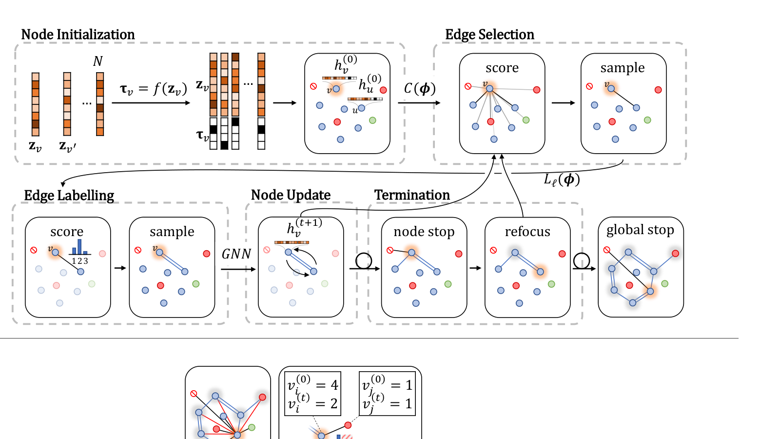
Our generative procedure is illustrated in Fig. 1. The process is seeded with vectors that together form a latent “specification” for the graph to be generated ( is an upper bound on the number of nodes in the final graph). Generation of edges between these nodes then proceeds using two decision functions: focus and expand. In each step the focus function chooses a focus node to visit, and then the expand function chooses edges to add from the focus node. As in breadth-first traversal, we implement focus as a deterministic queue (with a random choice for the initial node).
Our task is thus reduced to learning the expand function that enumerates new edges connected to the currently focused node. One design choice is to make expand condition upon the full history of the generation. However, this has both theoretical and practical downsides. Theoretically, this means that the learned model is likely to learn to reproduce generation traces. This is undesirable, since the underlying data usually only contains fully formed graphs; thus the exact form of the trace is an artifact of the implemented data preprocessing. Practically, this would lead to extremely deep computation graphs, as even small graphs easily have many dozens of edges; this makes training of the resulting models very hard as mentioned in mentioned in Li et al. (2018). Hence, we condition expand only upon the partial graph structure generated so far; intuitively, this corresponds to learning how to complete a partial graph without using any information about how the partial graph was generated. We now present the details of each stage of this generative procedure.
Node Initialization
We associate a state with each node in a set of initially unconnected nodes. Specifically, is drawn from the -dimensional standard normal , and is the concatenation , where is an interpretable one-hot vector indicating the node type. is derived from by sampling from the softmax output of a learned mapping where is a neural network11 1 We implement as a linear classifier from the dimensional latent space to one of the node type classes.. The interpretable component of gives us a means to enforce hard constraints during generation.
From these node-level variables, we can calculate global representations (the average representation of nodes in the connected component at generation step ), and (the average representation of all nodes at ). In addition to working nodes, we also initialize a special “stop node” to a learned representation for managing algorithm termination (see below).
Node Update
Whenever we obtain a new graph , we discard and compute new representations for all nodes taking their (possibly changed) neighborhood into account. This is implemented using a standard gated graph neural network (GGNN) for steps22 2 Our experiments use ., which is defined as a recurrent operation over messages .
Here the sum runs over all edges in the current graph and is an edge-type specific neural network33 3 In our implementation, is a dimension-preserving linear transformation. We also augment our model with a master node as described by Gilmer et al. (2017). Note that since is computed from rather than , the representation is independent of the generation history of .
Edge Selection and Labelling
We first pick a focus node from our queue. The function expand then selects edges from to with label as follows. For each non-focus node , we construct a feature vector , where is the graph distance between and . This provides the model with both local information for the focus node and the candidate edge (), and global information regarding the original graph specification () and the current graph state (). We use these representations to produce a distribution over candidate edges:
The factors are calculated as softmax outputs from neural networks (determining the target node for an edge) and (determining the type of the edge):44 4 and are fully connected networks with a single hidden layer of 200 units and ReLU non-linearities.
| (1) |
and are binary masks that forbid edges that violate constraints. We discuss the construction of these masks for the molecule generation case in Sect. 5.2. New edges are sampled from these distributions, and any nodes that are connected to the graph for the first time are added to the focus queue. Note that we only consider undirected edges in this paper, but it is easy to extend the model to directed graphs.
Termination
We keep adding edges to a node using expand and until an edge to the stop node is selected. Node then loses focus and becomes “closed” (mask ensures that no further edges will ever be made to ). The next focus node is selected from the focus queue. In this way, a single connected component is grown in a breadth-first manner. Edge generation continues until the queue is empty (note that this may leave some unconnected nodes that will be discarded).
4 Training the Generative Model
The model from Sect. 3 relies on a latent space with semantically meaningful points concentrated in the region weighted under the standard normal, and trained networks , , and . We train these in a VAE architecture on a large dataset of graphs. Details of this VAE are provided below.
4.1 Encoder
The encoder of our VAE is a GGNN that embeds each node in an input graph to a diagonal normal distribution in -dimensional latent space parametrized by mean and standard deviation vectors. The latent vectors are sampled from these distributions, and we construct the usual VAE regularizer term measuring the KL divergence between the encoder distribution and the standard Gaussian prior: .
4.2 Decoder
The decoder is the generative procedure described in Sect. 3, and we condition generation on a latent sample from the encoder distribution during training. We supervise training of the overall model using generation traces extracted from graphs in .
Node Initialization
To obtain initial node states , we first sample a node specification for each node and then independently for each node we generate the label using the learned function . The probability of re-generating the labels observed in the encoded graph is given by a sum over node permutations :
This inequality provides a lower bound given by the single contribution from the ordering used in the encoder (recall that in the encoder we know the node type from which was generated). A set2set model Vinyals et al. (2016) could improve this bound.
Edge Selection and Labelling
During training, we provide supervision on the sequence of edge additions based on breadth-first traversals of each graph in the dataset . Formally, to learn a distribution over graphs (and not graph generation traces), we would need to train with an objective that computes the log-likelihood of each graph by marginalizing over all possible breadth-first traces. This is computationally intractable, so in practice we only compute a Monte-Carlo estimate of the marginal on a small set of sampled traces. However, recall from Sect. 3 that our expand model is not conditioned on full traces, and instead only considers the partial graph generated so far. Below we outline how this intuitive design formally affects the VAE training objective.
Given the initial collection of unconnected nodes, , from the initialization above, we first use Jensen’s inequality to show that the log-likelihood of a graph is loosely lower bounded by the expected log-likelihood of all the traces that generate it.
| (2) |
We can decompose each full generation trace into a sequence of steps of the form , where is the current focus node and is the edge added at step :
The first term corresponds to the choice of as focus node at step of trace . As our focus function is fixed, this choice is uniform in the first focus node and then deterministically follows a breadth-first queuing system. A summation over this term thus evaluates to the constant .
As discussed above, the second term is only conditioned on the current graph (and not the whole generation history ). To evaluate it further, we consider the set of generation states of all valid state pairs of a partial graph and a focus node .

We use to denote the multiplicity of state in , i.e., the number of traces that contain graph and focus on node . Let denote all edges that could be generated at state , i.e., the edges from the focus node that are present in the graph from the dataset, but are not yet present in . Then, each of these appears uniformly as the next edge to generate in a trace for all occurrences of in a trace from ,
and therefore, we can rearrange a sum over paths into a sum over steps:
Here we use that is the probability of observing state in a random draw from all states in . We use this expression in Eq. 2 and train our VAE with a reconstruction loss ignoring additive constants.
We evaluate the expectation over states using a Monte Carlo estimate from a set of enumerated generation traces. In practice, this set of paths is very small (e.g. a single trace) resulting in a high variance estimate. Intuitively, Fig. 2 shows that rather than requiring the model to exactly reproduce each step of the sampled paths (orange) our objective does not penalize the model for choosing any valid expansion at each step (black).
4.3 Optimizing Graph Properties
So far, we have described a generative model for graphs. In addition, we may wish to perform (local) optimization of these graphs with respect to some numerical property, . This is achieved by gradient ascent in the continuous latent space using a differentiable gated regression model
where and are neural networks55 5 In our experiments, both and are implemented as linear transformations that project to scalars. and is the sigmoid function. Note that the combination of with (i.e., ) is exactly the GGNN regression model from Gilmer et al. (2017). During training, we use an distance loss between and the labeled properties . This regression objective shapes the latent space, allowing us to optimize for the property in it. Thus, at test time, we can sample an initial latent point and then use gradient ascent to a locally optimal point subject to an penalty that keeps the within the standard normal prior of the VAE. Decoding from the point then produces graphs with an optimized property . We show this in our experiments in Sect. 6.2.
4.4 Training objective
The overall objective is , consisting of the usual VAE objective (reconstruction terms and regularization on the latent variables) and the regression loss. Note that we allow deviation from the pure VAE loss () following Yeung et al. (2017).
5 Application: Molecule Generation
In this section, we describe additional specialization of our model for the application of generating chemical molecules. Specifically, we outline details of the molecular datasets that we use and the domain specific masking factors that appear in Eq. 1.
5.1 Datasets
We consider three datasets commonly used in the evaluation of computational chemistry approaches:
- •
QM9 (Ruddigkeit et al., 2012; Ramakrishnan et al., 2014), an enumeration of k stable organic molecules with up to 9 heavy atoms (carbon, oxygen, nitrogen and fluorine). As no filtering is applied, the molecules in this dataset only reflect basic structural constraints.
- •
ZINC dataset (Irwin et al., 2012), a curated set of 250k commercially available drug-like chemical compounds. On average, these molecules are bigger ( heavy atoms) and structurally more complex than the molecules in QM9.
- •
CEPDB (Hachmann et al., 2011; Hachmann et al., ), a dataset of organic molecules with an emphasis on photo-voltaic applications. The contained molecules have heavy atoms on average and contain six to seven rings each. We use a subset of the full database containing 250k randomly sampled molecules.
For all datasets we kekulize the molecules so that the only edge types to consider are single, double and triple covalent bonds and we remove all hydrogen atoms. In the encoder, molecular graphs are presented with nodes annotated with onehot vectors indicating their atom type and charge.
5.2 Valency masking
Valency rules impose a strong constraint on constructing syntactically valid molecules66 6 Note that more complex domain knowledge e.g. Bredt’s rule (Bredt et al., 1902) could also be handled in our model but we do not implement this here.. The valency of an atom indicates the number of bonds that that atom can make in a stable molecule, where edge types “double” and “triple” count for 2 and 3 bonds respectively. In our data, each node type has a fixed valency given by known chemical properties, for example node type “O” (an oxygen atom) has a valency of 2 and node type “O-” (an oxygen ion) has valency of 1. Throughout the generation process, we use masks and to guarantee that the number of bonds at each node never exceeds the valency of the node. If at the end of generation we link hydrogen atoms to node . In this way, our generation process always produces syntactically valid molecules (we define syntactic validity as the ability to parse the graph to a SMILES string using the RDKit parser Landrum (2014)). More specifically, also handles avoidance of edge duplication and self loops, and is defined as:
| (3) |
where is an indicator function, and as a special case, connections to the stop node are always unmasked. Further, when selecting the label for a chosen edge, we must again avoid violating the valency constraint, so we define , using to indicate single, double and triple bond types respectively
6 Experiments
We evaluate baseline models, our model (CGVAE) and a number of ablations on the two tasks of molecule generation and optimization77 7 Our implementation of CGVAE can be found at https://github.com/Microsoft/constrained-graph-variational-autoencoder..
6.1 Generating molecules
(a)
| Measure | 2: CGVAE | 3: Li et al. (2018) | 4: LSTM | 5: Gómez-Bombarelli et al. (2018) | 6: Kusner et al. (2017) | 7: Simonovsky and Komodakis (2018) | 8: Samanta et al. (2018) | |
|---|---|---|---|---|---|---|---|---|
| QM9 | % valid | 100 | - | 94.78 | 10.00 | 30.00 | 61.00 | 98.00 |
| % novel | 94.35 | - | 82.98 | 90.00 | 95.44 | 85.00 | 100 | |
| % unique | 98.57 | - | 96.94 | 67.50 | 9.30 | 40.90 | 99.86 | |
| ZINC | % valid | 100 | 89.20 | 96.80 | 17.00 | 31.00 | 14.00 | - |
| % novel | 100 | 89.10 | 100 | 98.00 | 100 | 100 | - | |
| % unique | 99.82 | 99.41 | 99.97 | 30.98 | 10.76 | 31.60 | - | |
| CEPDB | % valid | 100 | - | 99.61 | 8.30 | 0.00 | - | - |
| % novel | 100 | - | 92.43 | 90.05 | - | - | - | |
| % unique | 99.62 | - | 99.56 | 80.99 | - | - | - |
(c)
(b)
As baseline models, we consider the deep autoregressive graph model (that we refer to as DeepGAR) from Li et al. (2018), a SMILES generating LSTM language model with 256 hidden units (reduced to 64 units for the smaller QM9 dataset), ChemVAE Gómez-Bombarelli et al. (2018), GrammarVAE Kusner et al. (2017), GraphVAE Simonovsky and Komodakis (2018), and the graph model from Samanta et al. (2018). We train these and on our three datasets and then sample 20k molecules from the trained models (in the case of Samanta et al. (2018); Li et al. (2018), we obtained sets of sampled molecules from the authors).
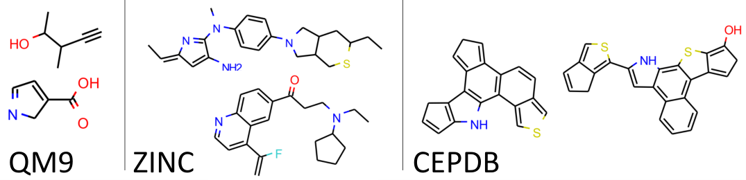
We analyze the methods using two sets of metrics. First in Fig. 3(a) we show metrics from existing work: syntactic validity, novelty (i.e. fraction of sampled molecules not appearing in the training data) and uniqueness (i.e. ratio of sample set size before and after deduplication of identical molecules). Second, in Fig. 3(b) we introduce new metrics to measure how well each model captures the distribution of molecules in the training set. Specifically, we measure the average number of each atom type and each bond type in the sampled molecules, and we count the average number of 3-, 4-, 5-, and 6-membered cycles in each molecule. This latter metric is chemically relevant because 3- and 4-membered rings are typically unstable due to their high ring strain. Fig. 3(c) shows 2 samples from our model for each dataset and we show more samples of generated molecules in the supplementary material.
The results in Fig. 3 show that CGVAE is excellent at matching graph statistics, while generating valid, novel and unique molecules for all datasets considered (additional details are found in supplementary material B and C). The only competitive baselines are DeepGAR from Li et al. (2018) and an LSTM language model. Our approach has three advantages over these baselines: First, whereas >10% of ZINC-like molecules generated by DeepGAR are invalid, our masking mechanism guarantees molecule validity. An LSTM is surprisingly effective at generating valid molecules, however, LSTMs do not permit the injection of domain knowledge (e.g. valence rules or requirement for the existance of a particular scaffold) because meaningful constraints cannot be imposed on the flat SMILES representation during generation. Second, we train a shallow model on breadth-first steps rather than full paths and therefore do not experience problems with training instability or overfitting that are described in Li et al. (2018). Empirical indication for overfitting in DeepGAR is seen by the fact that Li et al. (2018) achieves the lowest novelty score on the ZINC dataset, suggesting that it more often replays memorized construction traces. It is also observed in the LSTM case, where on average 60% of each generated SMILES string is copied from the nearest neighbour in the training set. Converting our generated graphs to SMILES strings reveals only 40% similarity to the nearest neighbour in the same metric. Third we are able to use our continuous latent space for molecule optimization (see below).
We also perform an ablation study on our method. For brevity we only report results using our ring count metrics, and other statistics show similar behavior. From all our experiments we highlight three aspects that are important choices to obtain good results, and we report these in ablation experiments A, B and C in Fig. 4. In experiment A we remove the distance feature from and see that this harms performance on the larger molecules in the ZINC dataset. More interestingly, we see poor results in experiment B where we make an independence assumption on edge generation (i.e. use features to calculate independent probabilities for all possible edges and sample an entire molecule in one step). We also see poor results in experiment C where we remove the GGNN from the decoder (i.e. perform sequential construction with ). This indicates that the choice to perform sequential decoding with GGNN node updates before each decision are the keys to the success of our model.
6.2 Directed molecule generation
Finally, we show that we can use the VAE structure of our method to direct the molecule generation towards especially interesting molecules. As discussed in Sect. 4.3 (and first shown by Gómez-Bombarelli et al. (2018) in this setting), we extend our architecture to predict the Quantitative Estimate of Drug-Likeness (QED) directly from latent space. This allows us to generate molecules with very high QED values by performing gradient ascent in the latent space using the trained QED-scoring network. Fig. 5 shows an interpolation sequence from a point in latent space with an low QED value (which ranges between 0 and 1) to the local maximum. For each point in the sequence, the figure shows a generated molecule, the QED value our architecture predicts for this molecule, as well as the QED value computed by RDKit.
| Pred. QED | 0.5686 | 0.6685 | 0.7539 | 0.8376 | 0.9013 | 0.9271 |
|---|---|---|---|---|---|---|
| Real QED | 0.5345 | 0.6584 | 0.7423 | 0.8298 | 0.8936 | 0.9383 |
7 Conclusion
We proposed CGVAE, a sequential generative model for graphs built from a VAE with GGNNs in the encoder and decoder. Using masks that enforce chemical rules, we specialized our model to the application of molecule generation and achieved state-of-the-art generation and optimization results. We introduced basic statistics to validate the quality of our generated molecules. Future work will need to link to the chemistry community to define additional metrics that further guide the construction of models and datasets for real-world molecule design tasks.
References
- Albert and Barabási [2002] R. Albert and A.-L. Barabási. Statistical mechanics of complex networks. Reviews of modern physics, 74(1):47, 2002.
- Allamanis et al. [2018] M. Allamanis, M. Brockschmidt, and M. Khademi. Learning to represent programs with graphs. In ICLR, 2018.
- Bredt et al. [1902] J. Bredt, J. Houben, and P. Levy. Ueber isomere dehydrocamphersäuren, lauronolsäuren und bihydrolauro-lactone. Berichte der deutschen chemischen Gesellschaft, 35(2):1286–1292, 1902.
- Defferrard et al. [2016] M. Defferrard, X. Bresson, and P. Vandergheynst. Convolutional neural networks on graphs with fast localized spectral filtering. In NIPS, 2016.
- Erdös and Rényi [1959] P. Erdös and A. Rényi. On random graphs, i. Publicationes Mathematicae (Debrecen), 6:290–297, 1959.
- Gilmer et al. [2017] J. Gilmer, S. S. Schoenholz, P. F. Riley, O. Vinyals, and G. E. Dahl. Neural message passing for quantum chemistry. arXiv preprint arXiv:1704.01212, 2017.
- Gómez-Bombarelli et al. [2016] R. Gómez-Bombarelli, J. Aguilera-Iparraguirre, T. D. Hirzel, D. Duvenaud, D. Maclaurin, M. A. Blood-Forsythe, H. S. Chae, M. Einzinger, D.-G. Ha, T. Wu, et al. Design of efficient molecular organic light-emitting diodes by a high-throughput virtual screening and experimental approach. Nature materials, 15(10):1120, 2016.
- Gómez-Bombarelli et al. [2018] R. Gómez-Bombarelli, D. K. Duvenaud, J. M. Hernández-Lobato, J. Aguilera-Iparraguirre, T. D. Hirzel, R. P. Adams, and A. Aspuru-Guzik. Automatic chemical design using a data-driven continuous representation of molecules. ACS Central Science, 4(2):268–276, 2018.
- Gori et al. [2005] M. Gori, G. Monfardini, and F. Scarselli. A new model for learning in graph domains. In IJCNN, 2005.
- [10] J. Hachmann, C. Román-Salgado, K. Trepte, A. Gold-Parker, M. Blood-Forsythe, L. Seress, R. Olivares-Amaya, and A. Aspuru-Guzik. The Harvard clean energy project database http://cepdb.molecularspace.org. http://cepdb.molecularspace.org.
- Hachmann et al. [2011] J. Hachmann, R. Olivares-Amaya, S. Atahan-Evrenk, C. Amador-Bedolla, R. S. Sánchez-Carrera, A. Gold-Parker, L. Vogt, A. M. Brockway, and A. Aspuru-Guzik. The harvard clean energy project: large-scale computational screening and design of organic photovoltaics on the world community grid. The Journal of Physical Chemistry Letters, 2(17):2241–2251, 2011.
- Irwin et al. [2012] J. J. Irwin, T. Sterling, M. M. Mysinger, E. S. Bolstad, and R. G. Coleman. Zinc: a free tool to discover chemistry for biology. Journal of chemical information and modeling, 52(7):1757–1768, 2012.
- Jin et al. [2018] W. Jin, R. Barzilay, and T. Jaakkola. Junction tree variational autoencoder for molecular graph generation. In Proceedings of the 36th international conference on machine learning (ICML), 2018.
- Johnson [2017] D. D. Johnson. Learning graphical state transitions. ICLR, 2017.
- Kingma and Welling [2013] D. P. Kingma and M. Welling. Auto-encoding variational bayes. arXiv preprint arXiv:1312.6114, 2013.
- Kipf et al. [2018] T. Kipf, E. Fetaya, K.-C. Wang, M. Welling, and R. Zemel. Neural relational inference for interacting systems. In ICML, 2018.
- Kipf and Welling [2017] T. N. Kipf and M. Welling. Semi-supervised classification with graph convolutional networks. ICLR, 2017.
- Kusner et al. [2017] M. J. Kusner, B. Paige, and J. M. Hernández-Lobato. Grammar variational autoencoder. CoRR, abs/1703.01925, 2017.
- Landrum [2014] G. Landrum. Rdkit: Open-source cheminformatics. http://www.rdkit.org, 2014.
- Leskovec et al. [2010] J. Leskovec, D. Chakrabarti, J. Kleinberg, C. Faloutsos, and Z. Ghahramani. Kronecker graphs: An approach to modeling networks. Journal of Machine Learning Research, 11(Feb):985–1042, 2010.
- Li et al. [2016] Y. Li, D. Tarlow, M. Brockschmidt, and R. Zemel. Gated graph sequence neural networks. ICLR, 2016.
- Li et al. [2018] Y. Li, O. Vinyals, C. Dyer, R. Pascanu, and P. Battaglia. Learning deep generative models of graphs. CoRR, abs/1803.03324, 2018.
- Neil et al. [2018] D. Neil, M. Segler, L. Guasch, M. Ahmed, D. Plumbley, M. Sellwood, and N. Brown. Exploring deep recurrent models with reinforcement learning for molecule design. ICLR workshop, 2018.
- Olivecrona et al. [2017] M. Olivecrona, T. Blaschke, O. Engkvist, and H. Chen. Molecular de-novo design through deep reinforcement learning. Journal of cheminformatics, 9(1):48, 2017.
- Qi et al. [2017] X. Qi, R. Liao, J. Jia, S. Fidler, and R. Urtasun. 3D graph neural networks for RGBD semantic segmentation. In Proceedings of the IEEE Conference on Computer Vision and Pattern Recognition, pages 5199–5208, 2017.
- Ramakrishnan et al. [2014] R. Ramakrishnan, P. O. Dral, M. Rupp, and O. A. Von Lilienfeld. Quantum chemistry structures and properties of 134 kilo molecules. Scientific data, 1:140022, 2014.
- Ruddigkeit et al. [2012] L. Ruddigkeit, R. Van Deursen, L. C. Blum, and J.-L. Reymond. Enumeration of 166 billion organic small molecules in the chemical universe database gdb-17. Journal of chemical information and modeling, 52(11):2864–2875, 2012.
- Samanta et al. [2018] B. Samanta, A. De, N. Ganguly, and M. Gomez-Rodriguez. Designing random graph models using variational autoencoders with applications to chemical design. CoRR, abs/1802.05283, 2018.
- Segler et al. [2017] M. H. Segler, T. Kogej, C. Tyrchan, and M. P. Waller. Generating focused molecule libraries for drug discovery with recurrent neural networks. ACS Central Science, 2017.
- Simonovsky and Komodakis [2018] M. Simonovsky and N. Komodakis. Towards variational generation of small graphs. In ICLR [Workshop Track], 2018.
- Snijders and Nowicki [1997] T. A. Snijders and K. Nowicki. Estimation and prediction for stochastic blockmodels for graphs with latent block structure. Journal of classification, 14(1):75–100, 1997.
- Vinyals et al. [2016] O. Vinyals, S. Bengio, and M. Kudlur. Order matters: Sequence to sequence for sets. ICLR, 2016.
- Weininger [1988] D. Weininger. Smiles, a chemical language and information system. 1. introduction to methodology and encoding rules. Journal of chemical information and computer sciences, 28(1):31–36, 1988.
- Yeung et al. [2017] S. Yeung, A. Kannan, Y. Dauphin, and L. Fei-Fei. Tackling over-pruning in variational autoencoders. arXiv preprint arXiv:1706.03643, 2017.
- You et al. [2018] J. You, R. Ying, X. Ren, W. L. Hamilton, and J. Leskovec. Graphrnn: A deep generative model for graphs. arXiv preprint arXiv:1802.08773, 2018.
Supplementary Material: CGVAE for Molecule Design
Appendix A Molecule Samples
We provide 25 random samples from our model for qualitative comparison with samples from each training dataset.
| Data Samples | CGVAE Samples | |
|
QM9 |
![[Uncaptioned image]](1805.09076v2/resources/samples/qm9_data_samples.png) |
![[Uncaptioned image]](1805.09076v2/resources/samples/qm9_samples.png) |
| ZINC | ![[Uncaptioned image]](1805.09076v2/resources/samples/zinc_data_samples.png) |
![[Uncaptioned image]](1805.09076v2/resources/samples/zinc_samples.png) |
| CEPDB | ![[Uncaptioned image]](1805.09076v2/resources/samples/cep_data_samples.png) |
![[Uncaptioned image]](1805.09076v2/resources/samples/cep_samples.png) |
Appendix B Effect of multiple training paths
Section 4.2 describes how we should enumerate all breadth first graph generation traces, break these traces into state transitions and then randomly sample state transitions to give the Monte Carlo estimate of the reconstruction loss. However, for computational efficiency, in the presented experiments we provide only a single trace containing transitions (where is the number of edges in the final molecule including edges to the stop node). Figure 6 shows an additional experiment (CGVAE (50)) where we enumerate 50 traces for each molecule and sample transitions from this enumeration (so the final dataset size is the same). While increasing the number of traces considered produces a small improvement in the matching of ring statistics in the sampled molecules, it is not clear that this benefit is worth the considerable computational overhead required in preparing the dataset.
Appendix C Additional Molecular Properties
Here we provide histograms of the following molecular properites of the sampled molecules for our method and the DeepGAR and LSTM baselines:
| Property | RDKit Implementation | Description |
|---|---|---|
| Molecular Weight | Chem.Descriptors.MolWt | The isotope-averaged molecular weight in atomic mass units. |
| Bertz Complexity | Chem.GraphDescriptors.BertzCT | A topological index meant to quantify complexity of molecules. |
| H donor count | Chem.Lipinski.NumHDonors | Number of heavy atoms bonded to H atoms that can form Hydrogen bonds. |
| H acceptor count | Chem.Lipinski.NumHAcceptors | Number of heavy atoms with lone electron pairs that can form Hydrogen bonds. |
| Rotatable bond count | Chem.Lipinski.NumRotatableBonds | Rotatable bonds are any single bond, not in a ring, bound to a nonterminal heavy atom. |
| Partition coefficient | Chem.Crippen.MolLogP | The octanol/water logP partition coefficient according to Wildman and Crippen 1999. |
| Topological polar surface area | Chem.rdMolDescriptors.CalcTPSA | The total exposed surface area of polar atoms in a molecule including attached Hydrogens (in square angstroms). |
![[Uncaptioned image]](1805.09076v2/extra_properties.png)
Appendix D Optimization trajectories
We provide additional QED optimization trajectories for our model trained on the ZINC dataset.
| Pred. QED | 0.5073 | 0.6249 | 0.6683 | 0.7375 | 0.8367 | 0.8927 |
|---|---|---|---|---|---|---|
| Real QED | 0.4419 | 0.5973 | 0.6789 | 0.7497 | 0.8186 | 0.8796 |
| Pred. QED | 0.4368 | 0.5046 | 0.7017 | 0.7683 | 0.8906 | 0.9427 |
|---|---|---|---|---|---|---|
| Real QED | 0.4188 | 0.5131 | 0.6910 | 0.7889 | 0.8709 | 0.9309 |