Energy Sustainable IoT with Individual QoS Constraints Through MISO SWIPT MulticastingThanks: D. Mishra is with the Division of Communication Systems, Department of Electrical Engineering (ISY), Linköping University, Linköping 58183, Sweden (e-mail: deepak.mishra@liu.se).Thanks: G. C. Alexandropoulos is with the Mathematical and Algorithmic Sciences Lab, Paris Research Center, Huawei Technologies France SASU, 92100 Boulogne-Billancourt, France (e-mail: george.alexandropoulos@huawei.com). Thanks: S. De is with the Department of Electrical Engineering and Bharti School of Telecommunication, Indian Institute of Technology Delhi, New Delhi 110016, India (e-mail: swadesd@ee.iitd.ac.in).Thanks: A preliminary version [1] of this work has been accepted for presentation at IEEE ICC, Kansas City, USA, May 2018.
Abstract
Enabling technologies for energy sustainable Internet of Things (IoT) are of paramount importance since the proliferation of high data communication demands of low power network devices. In this paper, we consider a Multiple Input Single Output (MISO) multicasting IoT system comprising of a multiantenna Transmitter (TX) simultaneously transferring information and power to low power and data hungry IoT Receivers (RXs). Each IoT device is assumed to be equipped with Power Splitting (PS) hardware that enables Energy Harvesting (EH) and imposes an individual Quality of Service (QoS) constraint to the downlink communication. We study the joint design of TX precoding and IoT PS ratios for the considered MISO Simultaneous Wireless Information and Power Transfer (SWIPT) multicasting IoT system with the objective of maximizing the minimum harvested energy among IoT, while satisfying their individual QoS requirements. In our novel EH fairness maximization formulation, we adopt a generic Radio Frequency (RF) EH model capturing practical rectification operation, and resulting in a nonconvex optimization problem. For this problem, we first present an equivalent semi-definite relaxation formulation and then prove it possesses unique global optimality. We also derive tight upper and lower bounds on the globally optimal solution that are exploited in obtaining low complexity algorithmic implementations for the targeted joint design. Analytical expressions for the optimal TX beamforming directions, power allocation, and IoT PS ratios are also presented. Our representative numerical results including comparisons with benchmark designs corroborate the usefulness of proposed framework and provide useful insights on the interplay of critical system parameters.
Index Terms:
Energy harvesting, internet of things, multicasting, multiple antennas, optimization, power allocation, power splitting, simultaneous wireless information and power transfer.I Introduction and Background
Wireless Energy Harvesting (EH) has been recently considered as a key technological concept for the energy sustainability of the Internet of Things (IoT) [2, 3]. An efficient technology belonging into this concept is the Simultaneous Wireless Information and Power Transfer (SWIPT) that targets at realizing perpetual operation of low power and data hungry network nodes [4, 5]. However, to achieve the goal of energy sustainable IoT via SWIPT, the fundamental bottlenecks of the practically available EH circuits need to be effectively handled. Among these bottlenecks are the low rectification efficiency in Radio Frequency (RF) to Direct Current (DC) conversion and the relatively low receive energy sensitivity [3]; the latter depends strongly on the distance between the Transmitter (TX) power node and a Receiver (RX) EH node. Recent advances in multiantenna signal processing techniques for SWIPT [6, 7, 8, 9, 10, 11, 12, 13, 14, 15, 16, 17, 18] have revealed that the effective exploitation of the spatial dimension has the potential to overcome EH bottlenecks both in point-to-point systems and in multipoint communication like IoT. Thus, SWIPT from a multiantenna TX has increased potential in providing continuous replenishment of the drained energy. However, novel low complexity designs are needed to optimize the harvested power fairness among IoT nodes, while meeting their Quality of Service (QoS) demands [19, 20].
I-A State-of-the-Art
In the seminal work [6] focusing on the efficiency optimization of point-to-point multiantenna SWIPT systems, the trade off between achievable rate and received power for EH (also known as rate-energy trade off) was investigated for practical RX architectures. Power Splitting (PS), Time Switching (TS), and Antenna Switching (AS) architectures were proposed with the latter two being special cases of the former. Further, spatial switching architecture was recently investigated for QoS-aware harvested power maximization in MIMO SWIPT system [21]. Based on these architectures, a lot of recent developments have lately appeared intending at enhancing the rate-energy performance of multiuser Multiple Input Single Output (MISO) SWIPT systems [7, 8, 9, 10, 11, 12, 13, 14, 15, 16, 17, 18, 22]. These works mainly target at the optimization of TX precoding and PS operation, and can be classified into the following two categories. The first category is based on whether RXs are required to perform both Information Decoding (ID) and EH (co-located ID and EH) [7, 8, 13, 10, 9, 12, 11, 14] or just act as ID or EH RXs (separated ID and EH) [15, 16, 17, 18]. The second category includes performance objectives like the minimization of TX power required for meeting Quality of Service (QoS) and EH constraints [7, 8, 10, 9, 11], and throughput [13, 15, 12, 14] or EH [17, 16, 18] maximization for a given TX power budget and QoS constraints. Recently in [22], the impact of the density of small-cell base stations together with their transmit power and the time allocation factor between EH and information transfer was analytically investigated for -tier heterogeneous cellular networks capable of SWIPT via TS. However, the jointly globally optimal TX precoding and RX PS operation for energy sustainable multiuser MISO SWIPT incorporating realistic nonlinear RF EH modeling is still unknown. Although the recent works [11, 14] considered nonlinear RF EH modeling for studying multiantenna SWIPT systems, analytical investigations on the joint designs and their efficient algorithmic implementation were not provided. More specifically, [11] considered that the harvested DC power is a known requirement at each EH-enabled RX, whereas [14] focused on a point-to-point multiantenna scenario.
I-B Paper Organization and Notations
Section II outlines the motivation and key contributions of this work. The considered system model description is presented in Section III, while Section IV details the proposed joint TX precoding and IoT PS optimization framework. Section V discusses the optimal TX precoding for the considered energy sustainable IoT problem formulation, and the Global Optimization Algorithm (GOA) along with analytical bounds for the unique global optimum are presented in Section VI. Tight closed form approximations for the optimal TX Power Allocation (PA) and RX PS ratios are presented in Section VII. A detailed numerical investigation of the proposed joint design along with the extensive performance comparisons against the relevant techniques is carried out in Section VIII. The concluding remarks are mentioned in Section IX.
Vectors and matrices are denoted by boldface lowercase and capital letters, respectively. The Hermitian transpose and trace of are denoted by and , respectively, and represents the identity matrix (). and denote the inverse and square root, respectively, of a square matrix , whereas means that is positive semi-definite. and are respectively used to represent the Euclidean norm of a complex vector and the absolute value of a complex scalar. and represent the complex and real number sets, respectively, and denotes the smallest integer larger than or equal to .
II Motivation and Key Contributions
In this paper we are interested in the energy sustainability of IoT systems comprising of low power and data hungry network nodes capable of EH functionality. Since the lifetime of an EH IoT system [23] depends on the time elapsed until the first EH network node runs out of energy, maximizing the minimum (max-min) energy that can be harvested among the nodes is critical. Focusing on a MISO SWIPT multicasting IoT system where a multiantenna TX is responsible for simultaneously transferring information and power to low power and data hungry EH PS RXs, we study the EH fairness maximization problem. Our proposed design aims at confronting the short wireless energy transfer range [2, 3] of the considered multicasting system by efficient utilization of the multiple TX antennas, thus, increasing the lifetime of RF EH IoT with individual QoS constraints. In our optimization formulation, we consider a generic RF EH model for the IoT nodes that captures the nonlinear relationship between the harvested DC power and the received RF power for any practically available RF EH circuit [24, 25, 26, 27]. Moreover, we consider the general case of individual QoS requirements for the IoT nodes, which are represented by respective Signal-to-Interference-plus-Noise Ratio (SINR) constraints. Our goal is to jointly design TX precoding and RX PS in order to maximize the minimum harvested energy among RXs, while satisfying their individual QoS constraints.
The EH fairness problem has been recently investigated for secure MISO SWIPT systems [28]. However, the existing TX precoding designs [6, 7, 8, 9, 10, 12, 13, 15, 16, 17, 18] adopted an oversimplified linear RF EH model which has been lately shown [26, 11, 14] to be incapable of capturing the operational characteristics of the available RF EH circuits. In addition, the designs in [6, 7, 8, 9, 10, 11, 12, 13, 14, 15, 16, 17, 18] are based either on numerical solutions or iterative algorithms. Proofs of global optimality or analytical solutions shedding insights on the interplay between different system parameters are in general missing. Motivated by these observations, in this paper we present an efficient algorithm for obtaining the jointly globally optimal TX precoding and IoT PS design for the considered optimization objective, and provide explicit analytical insights on the presented design parameters. The key distinctions of this work compared with the state-of-the-art are: the design objective that incorporates practical energy fairness IoT demands, a novel solution methodology taking into account the nonlinearity of RF-to-DC rectification operation, and the nontrivial analytical insights on the joint solution that eventually result in efficient low complexity sub-optimal designs.
Next we summarize the novel contributions of this work.
- •
We first present our novel EH fairness maximization problem for energy sustainable MISO SWIPT multicasting IoT systems, while incorporating the practical nonlinear RF-to-DC rectification process. This nonconvex optimization problem is then transformed to an equivalent Semi-Definite Relaxation (SDR) formulation and we prove that it possesses a unique global optimum.
- •
We derive analytical tight upper and lower bounds for the global optimal value of the considered optimization problem. Capitalizing on these bounds, we then present an iterative GOA for the computation of the jointly globally optimal TX precoding and IoT PS ratios design. The fast convergence of the proposed algorithm to the global optimum of the targeted problem has been both analytically described and numerically validated.
- •
We present analytical insights for the optimal TX beamforming directions by investigating the interplay between the directions for either solely optimizing EH performance or the ID one. Tight analytical approximations for the optimal TX PA and uniform PS ratio at each IoT node for a given TX precoding design are also derived. The latter insights and approximations have been used for designing two low complexity sub-optimal algorithms. These low complexity designs are suitable for low power IoT nodes and exhibit performance sufficiently close to the optimum one for certain cases of practical interest.
- •
Our numerical results gain insights on the impact of key system parameters on the trade-off between optimized received RF power for EH at each node and their individual QoS requirements. We also carry out extensive comparative numerical investigations between our presented designs and relevant benchmark schemes which corroborate the utility of our optimization framework.
The key challenges addressed in this paper for the considered MISO SWIPT multicasting IoT systems are: (a) incorporation of nonlinear RF-to-DC rectification operation in the proposed jointly globally optimal TX precoding and IoT PS ratio design; and (b) derivation of efficient (sufficiently close to the optimum for certain cases of practical interest) low complexity joint designs addressing the limited computational capability and energy constraints of low power IoT nodes.
III System Description
In this section we first present the considered MISO SWIPT multicasting IoT system together with the adopted channel model and underlying signal model. Then, we introduce the generic RF EH model under consideration that is capable of capturing the rectification operation of realistic RF EH circuits.
III-A System and Channel Models
We consider a MISO SWIPT multicasting IoT system comprising of single-antenna IoT nodes and one sink node equipped with antennas that is responsible for simultaneously transferring information and power to the IoT nodes. Hereinafter, each -th IoT node is denoted by RXk and the sink node is termed for simplicity TX. The multiantenna TX adopts Space Division Multiple Access (SDMA) with linear precoding according to which each RXk is assigned a dedicated precoding vector (or beam) for SWIPT. We denote by the unit power data symbol at TX, which is chosen from a discrete modulation set and intended for RXk. These data symbols are transmitted simultaneously through spatial separation with the aid of the linear precoding vectors . As such, the complex baseband transmitted signal from the multiantenna TX is given by . For each precoding vector associated with the data symbol , we distinguish its following two components: i) The phase part given by the normalized beamforming direction ; and ii) The amplitude part representing the power allocated to , i.e., . Combining the latter two components of each yields . For the transmitted signal , we assume that there exists a total power budget , hence, it must hold .
A frequency flat MISO fading channel is assumed for each of the wireless links that remains constant during one transmission time slot and changes independently from one slot to the next. We represent by the channel vector between the -antenna TX and the single-antenna RXk. The entries of each are assumed to be independent Zero-Mean Circularly Symmetric Complex Gaussian (ZMCSCG) random variables with variance that depends on the propagation losses of the TX to RXk transmission. The baseband received signal at RXk can be mathematically expressed as
| (1) |
where represents the zero-mean Additive White Gaussian Noise (AWGN) with variance . Assuming the availability of perfect Channel State Information (CSI) at both TX and RXs, we consider PS receptions [6] according to which each RXk splits its received RF signal with the help of a power splitter. Particularly, an fraction of the received RF power at RXk is used for ID and the remaining fraction is dedicated for RF EH. Using this definition in (1), the received signal available for ID at RXk is given by
| (2) |
where is a ZMCSCG distributed random variable with variance representing the additional noise introduced during ID at RXk. The resulting SINR for at each RXk can be derived as
| (3) |
where Similarly, the corresponding received signal available for RF EH at each RXk is given by
| (4) |
Using the latter expression, the total received RF power at each RXk that is available for EH is defined as
| (5) |


III-B RF Energy Harvesting Model
The harvested DC power at each RXk after RF-to-DC rectification of the received signal is given using (5) by
| (6) |
where represents the received RF power at RXk and denotes the RF-to-DC rectification efficiency function of the RF EH circuitry used at each of the RXs. In general, is a positive nonlinear function of the received RF power available for RF EH [24, 25, 26, 27]. This function is plotted in Fig. 1(a) for two real-world RF EH circuits, namely, the commercially available Powercast P1110 Evaluation Board (EVB) [24] and the circuit designed in [25] for low power far field RF EH. It is obvious that the widely considered [6, 7, 8, 9, 13, 15, 17, 16, 18, 28] trivial linear RF EH model cannot efficiently describe practical rectification functionality, hence very recently, nonlinear models have been proposed [26, 27]. Despite the nonlinear relationship between the rectification efficiency and , we note that due to the law of energy conservation holds that at each RXk is monotonically increasing with , as shown in Fig. 1(b). Hence, although the form of differs for different RF EH circuits, the non-decreasing nature of with is valid for all practical RF EH circuits [25]. In other words, the relationship between the harvested DC power and received RF power can be defined as , where represents a nonlinear non-decreasing function. We will exploit this feature in the following section including our proposed joint TX precoding and IoT PS optimization formulation.
IV Optimization Problem Formulation
We first present our energy sustainable IoT problem formulation and describe its key mathematical properties. Then, we present an equivalent SDR formulation for this problem and prove that it possesses a unique global optimum. We finally discuss the problem’s feasibility conditions.
IV-A Problem Definition
We are interested in the joint design of TX precoding vectors and RXs’ PS ratios that maximizes the minimum of among the RF EH RXs, while satisfying all the underlying minimum SINR requirements of all RXs. By using (3), (6), and the total TX power , the proposed optimization problem for the considered MISO SWIPT multicasting IoT system is formulated as
where constraints and represent the minimum SINR requirements and maximum TX power budget, respectively. In addition, constraint includes the boundary conditions for ’s. is a nonlinear nonconvex combinatorial optimization problem including the nonlinear function in the objective along with the coupled vectors and ratios in both the objective and constraints. Specifically, quadratic terms of appear in both the objective and constraints. To resolve these non tractable mathematical issues, we next present an equivalent SDR formulation for that can be solved optimally. Also, since RXs in the considered system are energy constrained, we assume that is solved at TX using the foreknown SINR demands along with the CSI knowledge of all involved links. After computing the optimal PS ratios, they are communicated to the corresponding RXs via appropriately designed control signals.
IV-B Semi-Definite Relaxation (SDR) Transformation
Using the definition in and ignoring the rank- constraint for each , an equivalent formulation can be obtained after applying some algebraic rearrangements to the constraints and objective of , as follows:
Constraints and represent the equivalent transformations for and , respectively. We have particularly replaced the TX precoding vectors with their respective matrix definition . An additional variable has been also included to reformulate the max-min problem to the simpler maximization problem having additional constraints, as represented by the new constraint . We have also replaced the harvested power maximization problem in with the corresponding received RF power for EH maximization in by using the two key results as discussed next in Lemmas 1 and 2.
Lemma 1
The power at each RXk is jointly pseudoconcave in and .
Proof:
The product of the two positive linear functions and that defines the received RF power for EH at RXk is a pseudoconcave function [29, Tab. 5.3]. This pseudoconcavity property holds jointly for in the expression (5) and . ∎
Lemma 2
The max-min problem of among the RXs is equivalent to the problem of maximizing the corresponding minimum received RF powers .
Proof:
From the discussion in Sec. III-B it follows that each harvested DC power is a non-decreasing function of the corresponding . It also holds that the non-decreasing transformation of the pseudoconcave function is pseudoconcave [29, 30]. Using these properties together with Lemma 1, we conclude that, since is jointly pseudoconcave in and , the same holds for . In addition, it is known that a pseudoconcave function has a unique global maximum [31, Chap. 3.5.9]. Hence, maximizing the minimum among is equivalent to maximizing the minimum among , and function defines the mathematical formula connecting their globally optimal solutions. ∎
Using the latter two lemmas, we next prove the generalized convexity of along with its equivalence to .
Theorem 1
having the unique globally optimal solution is an equivalent formulation for .
Proof:
We first show that belongs to the special class of generalized convex problems [31, Chapter 4.3] that possess the unique global optimality property. Actually, and in are linear (i.e., convex) constraints. Due to the linearity of the expression and the convexity of in and , is jointly quasiconvex. In addition, is jointly pseudoconcave from Lemma 1. Combining these properties of constraints along with the linearity of objective and result in [31, Theorem 4.3.8], yields that the Karush Kuhn Tucker (KKT) point of is its globally optimal solution.
It follows from Lemma 2 that the harvested DC power max-min problem is equivalent to maximizing the minimum among the received RF powers. Using this result together with the epigraph transformation [30, Chap. 4.2.4] of , we obtain with an implicit rank- constraint to be satisfied by the globally optimal TX precoding matrix . As it will be proven in the following lemma, this condition is always implicitly met. Hence, and are equivalent and the globally optimal solution of can be obtained from the globally optimal solution of , where the optimal TX precoding vector for each RXk is derived from the EigenValue Decomposition (EVD) of . ∎
Lemma 3
The optimal solution of implicitly satisfies the rank- condition for .
Proof:
Keeping constraints and in implicit and associating the Lagrange multipliers , , and , respectively, with the constraints , , and , the Lagrangian function of is defined as
| (7) |
with and . As and , it holds . Using this function, the dual function of is given by
| (8) |
Since has a unique globally optimal solution (cf. Theorem 1), it holds from the strong duality principle [31, Section 6.2] that its solution can be also obtained from the solution of the following dual problem:
Denoting the optimal solution of as , the optimal power and that maximize the Lagrangian in (7) is the optimal solution of . Since the variables are decoupled from the remaining variables and as shown in (7), we can compute by solving the following equivalent problem (note that constant terms have been discarded in this equivalent formulation):
| (9) |
In (9), and are obtained by substituting the optimal solutions of into and , respectively. Here we have implicitly used and , where the latter is imposed in order to have a bounded solution for . Using these properties along with the results proved in [8, Prop. 1] (or [17, Th. 1]), the rank- property of the optimal solution of (9) can be shown by contradiction. Hence, each has to be a rank- matrix like . ∎
Remark 1
The outcomes of our energy sustainable IoT problem formulation that focuses on the practical QoS-aware harvested power fairness maximization are different from the objectives in existing multiuser SWIPT works [7, 8, 9, 10, 11, 12, 13, 14, 15, 16, 17, 18]. This will be shown analytically in Section V and through numerical validations in Section VIII. The same holds for the joint TX precoding and IoT PS design of the proposed optimization problem that will be presented in the following sections.
IV-C Feasibility Conditions
The feasibility of depends on the underlying SINR constraints of all RXs that need to be simultaneously met for a given total TX power budget . To check whether can be satisfied, we solve the following problem:
, which does not consider EH (i.e., for each RXk), has been widely studied and its globally optimal solution denoted by is given by [32, eq. (10)]. If , then both and are feasible, otherwise they are not. Also, to ensure in , needs to satisfy , where is the receive energy sensitivity of the RF EH circuit [3, 25].
V Optimal TX Precoding Design
Here we provide insights on the optimal TX precoding design for our energy sustainable IoT problem. These insights will be used later for implementing efficient algorithms for the jointly global optimal TX precoding and IoT PS design.
V-A Optimal TX Precoding Structure
The Lagrangian function of given by (7) can be rewritten in terms of the precoding vectors as
| (10) |
Then, from Theorem 1, each optimal can be derived by solving (KKT condition for optimal TX precoding vector), which after few algebraic manipulations simplifies to
| (11) |
Since in (11) is a scalar, the optimal beamforming direction for each RXk can be obtained as
| (12) |
The Lagrange multipliers and in (12) respectively correspond to the constraints and , and are respectively related to the EH and SINR requirements for RXk. When , coincides with the optimal TX precoding for ID (i.e., no EH) as given by [32, eq. (10)]. Whereas, yields , which refers to Maximal Ratio Transmission (MRT) for RXk. Therefore, the structure of is a modified version of the regularized Zero Forcing (ZF) beamformer [9] that balances the trade off between minimizing interference solely for efficient ID and maximizing the intended signal strength for efficient EH.
V-B TX Precoding Design
As noted in the above discussion, the optimal TX beamforming direction needs to balance the trade-off between the beamforming directions intended for (i) maximizing the harvested energy fairness and (ii) the one targeting efficient information transfer by meeting the SINR demands with minimum required TX power budget. Capitalizing this insight we propose the following weighted TX beamforming direction:
| (13) |
where represents the relative weight between the TX beamforming direction for efficient ID and the corresponding direction for efficient EH. We next derive the latter directions from their respective optimal TX precoding vectors and , respectively.
V-B1 Energy Fairness Maximization (EFM)
By setting (i.e., no ID requirement at RXs) in , we focus solely on maximizing the EH fairness of the considered multicasting IoT system. For this setting, reduces to the following EH fairness optimization problem:
Since, has a linear objective and constraints, it is convex. Let denote its jointly optimal solution.
Corollary 1
The optimal solution of implicitly satisfies the rank- condition for . Hence, for each RXk is derived from the EVD of .
Proof:
Keeping constraint in implicit and associating the Lagrange multipliers and with the constraints and , respectively, the Lagrangian function of is defined as
| (14) |
where . Following similar steps to the proof of Lemma 3, the optimal precoding can be obtained by solving the equivalent problem defined below:
| (15) |
where and are obtained by substituting the optimal solutions of the dual problem for into and . Lastly, using and along with the results in Lemma 3, the rank- properties of the optimal solution of (15), and thus that of in , can be shown by contradiction. ∎
Remark 2
V-B2 Information Decoding (ID)
When solely targeting TX precoding for enhancing the ID performance, we consider the case (i.e., no EH requirement at RXs). To derive , we focus on solving as defined in Section IV-C that seeks for the precoding design minimizing the total TX power, while meeting the individual SINR requirements. Also, is feasible only if .
In the following section we present an iterative GOA for that utilizes the optimal TX precoding vectors and .
VI Joint TX Precoding and RX Power Splitting
Although exhibits generalized convexity as shown in Section IV-B, standard optimization tools (e.g., the CVX Matlab package [33]) cannot be used due to the fact that constraint does not satisfy the Disciplined Convex Programming (DCP) rule set; this constraint includes the coupled term . To resolve this issue, we summarize in the sequel an iterative GOA for solving that capitalizes on our derived tight upper and lower bounds for the optimal of and uses and of Section V-B.
VI-A Tight Analytical Bounds for the Optimal in
VI-A1 Upper Bound on
Clearly, the optimal solution of as defined in Section V-B1, provides an upper bound for because there is no SINR constraint to be met. However, we next present a tighter upper bound that can be obtained from the solution of the following problem:
In , we seek for the minimum TX power required to meet together with the SINR demands . The objective and constraints of this problem are jointly convex in with satisfying the rank- constraint. In addition, satisfies the DCP rule set, hence, we can efficiently compute its jointly optimal solution using [33]. The tight upper bound for can thus be obtained as
| (16) |
Note that, due to the presence of in and along with the fact that and , it holds that .
VI-A2 Lower Bound on
With , is feasible and its solution can be lower bounded as
| (17) |
To find a tighter lower bound, we then set in and denote its jointly optimal solution by . The lower upper bound for can be then derived using the solution of as
| (18) |
Lastly, since and , it yields .
Note that the tightness of the presented lower and upper bounds will be later numerically validated in Section VIII.
VI-B Global Optimization Algorithm (GOA)
The proposed GOA for efficiently solving is based on one-dimensional Golden Section Search (GSS) over the feasible range of values, as given by the previously derived bounds and . Its detailed algorithmic steps for the case where is feasible are outlined in Algorithm 1. Due to the generalized convexity of and the tightness of and , the proposed GOA converges fast to the optimal satisfying the TX power budget expressed by constraint within an acceptable tolerance .
Complexity Analysis
We now discuss the computational time required to obtain the joint TX precoding design and IoT PS ratios for through GOA presented in Algorithm 1. According to this algorithm, are outputted when the resulting is close up to the acceptable tolerance to ’s globally optimal value. As seen from Algorithm 1, the search space interval after each GSS iteration reduces by a factor of [34, Chap. 2.5]. This value combined with the quantity as the maximum search length for gives the total number of iterations that are required for the termination of Algorithm 1, while ensuring that the numerical error is less than . Putting all together, we need to solve the problems and separately along with the runs for solving to eventually obtain the jointly globally optimal solution of , and consequently due to equivalence. However, as will be numerically shown later on in Section VIII (cf. Fig. 6), since holds , is generally very low in practice and corroborates the fast convergence of Algorithm 1.
GOA provides an efficient way to obtain the joint TX precoding and IoT PS design for , however, analytical insights on the jointly globally optimal parameters are difficult to be extracted. Recall that and that analytical insights on each beamforming direction were presented in Section V. We next present two sub-optimal designs that are based on the weighted TX beamforming directions given by (13) and exhibit low complexity computation of the weights , the PA , and IoT PS ratios . It will be shown in the results later on that, for high values of the SINR demands, the sub-optimal algorithms perform sufficiently close to GOA, returning globally optimal solution.
VII Sub-optimal Precoding and Power Splitting
In this section we first present two jointly optimal PA and IoT PS schemes for given TX beamforming directions. The one assumes possibly different PS ratios among RXs and is termed as Dynamic Power Splitting (DPS), and the other considers Uniform Power Splitting (UPS). Capitalizing on these schemes, we then introduce two low complexity sub-optimal designs for the weights of the proposed weighted TX beamforming directions described in Section V-B.
VII-A Power Allocation (PA) and Dynamic Power Splitting (DPS)
Given the beamforming directions and considering possibly different PS ratios among RXs, reduces to the following joint TX PA and RX PS design problem:
The generalized convexity [31, Chapter 4.3] of can be proved in a similar fashion to . The objective of is linear, constraints , , and are convex, and together with possess joint quasiconvexity in . Based on this property, ’s globally optimal solution can be obtained from the solution its KKT conditions. We thus associate the Lagrange multipliers , , and , respectively, with , , and , while keeping and implicit. Hence, the Lagrangian of is given by
| (19) |
Together with constraints – and the requirement for positive Lagrange multipliers, the KKT conditions for are given by
| (20a) | ||||
| (20b) | ||||
| (20c) | ||||
| (20d) | ||||
| (20e) | ||||
| (20f) | ||||
Since, power received at each RXk intended for EH is an increasing function of , the TX power budget constraint is always satisfied at equality, thus causing due to complimentary slackness condition, as defined in (20d). We also observe from (20a), (20b), and (20c) that if , then . Applying the latter result in (20f) yields
| (21) |
which can be rewritten in matrix form as follows
where the elements of are defined as
| (30) |
By substituting (VII-A) into (20e) and applying some mathematical simplifications, we obtain the following equations:
| (31) |
The optimal PS ratios and RF power for EH, as respectively denoted by and , are finally obtained by solving a system of equations, particularly, the first equations of (31) together with the following equation:
| (32) |
The latter equation results from the substitution of (VII-A) into . Since it holds as well as (in W) due to wireless propagation characteristics and the low energy sensitivity of practical RF EH circuits (typically dBm [25]), the system of equations can be solved efficiently using commercial numerical solvers (like Matlab and Mathematica). This holds true due to the small search space the unknown parameters lie. Finally, the optimal PA is obtained by substituting into (VII-A).
VII-B Power Allocation (PA) and Uniform Power Splitting (UPS)
Given the beamforming directions and considering UPS for all RXs, yields after substitution into (32)
| (33) |
The optimal UPS is obtained from the latter equation as
| (34) |
Using this value in (VII-A) and (31) the optimal PA and the optimal RF power for EH are, respectively, given by
| (35a) | |||
| (35b) | |||
Obviously, for this case of given TX beamforming directions and UPS, the jointly optimal PA and UPS design is obtained in closed form as defined in (35a) and (34) with corresponding optimal RF power for EH as given by (35b).
VII-C Low Complexity Sub-optimal Designs
We next present two iterative schemes for computing the weights of the weighted TX beamforming directions given by (13), which together with the previous joint PA and IoT PS schemes comprise our two proposed low complexity sub-optimal designs for . Their low complexity comes from the fact that, for given TX beamforming directions, the jointly optimal PA and IoT UPS is obtained in closed form as shown in Section VII-B (i.e., using (34), (35a) and (35b)) and in an efficient way as presented in Section VII-A (i.e., by solving (31) and (32)) for the DPS case.
VII-C1 Uniform Weight Allocation (UWA)
In the UWA scheme it is considered that . Without loss of generality, we assume that the common varies in discrete steps ranging from to , resulting in the weight allocation . To compute yielding the maximum , one needs to evaluate for all assumed allocations and then select the best among them.
VII-C2 Distinct Weight Allocation (DWA)
For this scheme we consider that each weight varies in discrete steps. Instead of performing dimensional traverses over the possible weight allocations that imposes increased complexity, we first sort the values for all RXs. Then, we proceed by optimizing the weight for the RX having the lowest channel gain (i.e., RXi for which ), while setting unit weights for all other RXs (i.e., , which means that for these RXs ID is solely chosen). The optimization continues by selecting the weight that results in the highest among the possible weight allocations for the current RX. At most discrete weight allocations need to be checked till obtaining yielding the maximum .
VIII Numerical Results and Discussion
In this section we evaluate the presented joint TX precoding and IoT PS designs for the considered MISO SWIPT multicasting IoT system. In figures that follow we have set W, , dBm, dBm, dBm, , , and in certain cases . In addition, with being the average channel attenuation at unit reference distance, is TX to RXk distance, and is the path loss exponent. The RXs have been placed uniformly over a square field with length m and the TX was placed at its center. For the average performance results included in the figures we have used independent channel realizations.
VIII-A Energy Harvesting vs SINR Tradeoff
We first plot in Fig. 2 the average optimal received RF power for EH via GOA as a function of values in dB for different combinations of and . This plot is also known as EH power versus SINR tradeoff. As shown, lower (i.e., lesser propagation loss) and higher (i.e., larger beamforming gain) values improve this tradeoff. It is also observed that as increases from dB to dB, there is a lower decrease of about dBm in for as compared to the decrease of dBm for . Recall that RXs have been considered. This corroborates the utility of having more TX antennas for improved EH power versus SINR tradeoff. In addition, for the case of field size m, is about dBm lower than that for m.

Within this figure, we also sketch the obtained tradeoff for the sub-optimal design using UPS (i.e., ). This design performs very close to the sub-optimal DPS one that optimizes the individual PSs exhibiting lower complexity. Recall that with the UPS-based design the jointly optimal PA and UPS are obtained in closed form, and the TX beamforming weights are computed via a simple one-dimensional search.

The role of the number of TX antennas in performance using GOA is depicted in Fig. 3 for different combinations of and (or ) values. Increasing from to improves at each of the RXs by about dBm. As expected due to the low energy transfer efficiency of SWIPT systems, the lower field size m yields larger at dB as compared to that of m at dB. For the case of unequal SINR demands at the RXs, we have used the values , , , and , with mean among them being the common SINR value or dB. Likewise, for the common SINR being mean value (or dB), we have set , , , and . Although a similar trend happens in both distinct SINR scenarios, it is noted that they both result in an average increase of about % in the average received RF power for EH as compared to the scenario having the same SINR demands for all four RXs.

In Fig. 4 we investigate the effect of IoT density for the parameter setting of Fig. 3 expect for assuming and varying the number of RXs . It can be observed that degrades significantly as the TX load to transfer energy to more RXs increases.


The impact of the nonlinear rectification efficiency on the optimized harvested DC power with varying number of RXs is showcased in Fig. 5 for the case where the RF EH unit of each RX is the Powercast P1110 EVB [24]. The results for and , as respectively plotted in Figs. 5(a) and 5(b), are obtained using the relationship between and for the considered board, which has been analytically characterized by [27, eq. (6)]. Unlike the variation of with , follows a monotonically decreasing trend with increasing , a trend that is actually very similar to the one followed by in Fig. 4. This corroborates the discussion with respect to the claims made in Lemma 2 and the RF EH characteristics as plotted in Fig. 1.

To corroborate the fast convergence of the proposed GOA in Algorithm 1, we illustrate in Fig. 6 the difference between our derived lower and upper bounds along with the optimal for RXs and different values of and . It can be shown that the search space for is very small (i.e., ). Particularly, the average difference between and is less than mW (or dBm) for dB and less than mW (or dBm) for dB. This fact validates our claims for the quality of our presented bounds for and the fast convergence of GOA to the jointly globally optimal TX precoding and IoT PS design.
VIII-B Optimal TX Beamforming Direction, PA, and RX PS Ratios
We now focus on our two presented low complexity sub-optimal schemes in Section VII-C and investigate the derived designs for the TX beamforming directions and PA (combinedly forming the TX precoding design) as well as the RX PS ratios under different system parameter settings.
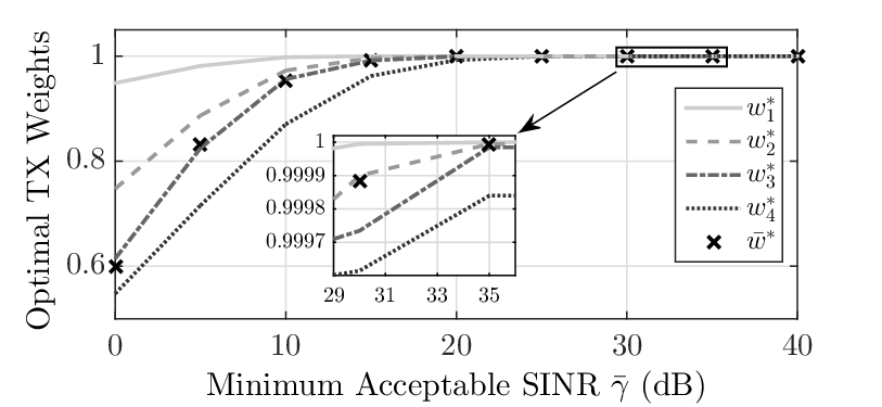
In Fig. 7 we first plot the optimal weights versus in dB that are assigned to the weighted TX beamforming directions given by (13) using the proposed iterative DWA scheme. For this figure we have considered and m. As shown, each weight increases with increasing SINR demand. This implies that the relative importance of TX precoding for efficient ID alone (as represented by ) gets significantly higher than the precoding designed for maximizing the EH performance (as represented by ). In addition, it can be seen that the weight values in this figure are mainly approaching their largest values (i.e., greater than even for dB). This shows that the designed TX beamforming directions approaching the optimal ones from GOA are closer to the ID-based TX precoding (i.e., ).

We now use the parameter setting of Fig. 7 and the derived TX beamforming directions to plot in Fig. 8 the variation of the optimal TX PA for both the DPS and UPS schemes. As shown for high SINR demands (i.e., for dB), and for UPS and DPS closely match among each other. This trend again corroborates the fact that the adoption of the UPS scheme is a good approximation for MISO SWIPT multicasting IoT systems with high QoS constraints. It is also evident that for high SINR values the optimal PA becomes independent of the variations.

The optimal PS ratios using both DPS and UPS schemes is illustrated in Fig. 9 as a function of the SINR in dB for as well as m and m. For dB the optimal PS ratios and with DPS increase with increasing . Interestingly, all ratios become nearly equal for dB and match very closely with the optimal UPS ratio . This again showcases that the UPS-based scheme provides a very good approximation for the DPS one, especially for high QoS constraints. However, at the low SINR regime, the optimal DPS-based PS ratios follow a different trend from the UPS one. This has been also noticed in Figs. 7 and 8 where power allocations and TX precoding for these two schemes were designed as different.
VIII-C Comparisons with Relevant Designs
The proposed joint TX precoding and IoT PS design will be compared next with benchmark designs available in the relevant literature [7, 9, 16]. As shown in the previous figures, our joint design based on the UPS scheme exhibits low complexity computation of the involved parameters and performs sufficiently close to our optimal joint design obtained from GOA. This low computational overhead is achieved using the closed form expressions for PA and UPS, along with a simpler one-dimensional search for obtaining the TX beamforming weights. We will thus consider this scheme in the performance comparisons that follow incorporating either the UWA or the DWA technique for the TX beamforming weight computation. We term these two versions of our joint design as Proposed-UWA-UPS and Proposed-DWA-UPS, respectively. For the benchmark designs we use the terminology SINR-UPS for the design in [7], as well as MRT-ZF-UWA-UPS and MRT-ZF-DWA-UPS for those in [9].

In Fig. 10 we plot the received RF power for EH in mW versus in dB for , m, and for all under comparison designs. It is evident that both our proposed low complexity designs and SINR-UPS significantly outperform MRT-ZF-UWA-UPS and MRT-ZF-DWA-UPS. The gap averaged over all SINR demands between the EH power achieved by DWA and UWA is less than dBm, in other words, the average improvement of DWA over UWA is around . This gap between DWA and SINR-UPS is around dBm, hence, the corresponding average improvement is around .

In Fig. 11 we plot the optimal UPS ratio versus in dB for our two proposed designs and SINR-UPS considering , m, and different values. It is obvious that is very similar for all three designs, a fact that justifies their similar achieved EH power in Fig. 10.

The performance comparison of our GOA and low complexity sub-optimal designs together with SINR-UPS is included in Fig. 12, where , m, and different values for in dB and have been considered. As shown, GOA provides for an average improvement of about and over the Proposed-DWA-UPS, Proposed-UWA-UPS, and SINR-UPS designs, respectively, in terms of achievable RF power for EH. When the number of TX antennas increases to , this performance enhancement slightly reduces to and , respectively. Obviously, despite the relatively high GOA complexity, this algorithm provides sufficient performance improvement for low and medium vales of the SINR demands. However, for high SINR demands, this performance improvement is not as significant. One may also notice that the proposed design adopting DWA that requires computations does not provide significant improvement over that based on UWA that requires only computations. In addition, its is shown in the last two figures that the Proposed-UWA-UPS design outperforms SINR-UPS with an average performance improvement of around .

In Fig. 13 we finally compare for and different values the received RF power for EH obtained using our proposed EFM TX precoding design presented in Section V-B1, the MRT design of [9], and the TX energy beamforming design of [16] that is based on the Singular Value Decomposition (SVD) of the concatenated channel matrix for all RXs. As observed, MRT performs close to our proposed design exhibiting a mean performance degradation of about dBm. The SVD design, however, that targets at maximizing the sum RF power for EH performs very poor in terms of EH fairness performance. We thus conclude that not only our proposed joint TX precoding and IoT PS design provides significant improvements over the existing competitive benchmarks schemes, but even our proposed EFM TX precoding designs yields significant energy savings over relevant ones.
IX Conclusions
In this paper, we investigated the max-min EH fairness problem in MISO SWIPT multicasting IoT systems comprising of PS IoT devices having individual QoS constraints. A generic RF EH model that captures practical rectification operation was adopted. We first obtained an equivalent SDR formulation for the considered design problem and then presented an efficient algorithmic implementation for the jointly globally optimal TX precoding and IoT PS ratio parameters. It was shown that each optimal TX precoding vector has a special regularized ZF structure, based on which a novel weighted TX beamforming direction was proposed for serving each IoT device. Tight closed form approximations for the optimal TX PA allocation and RX UPS ratio were derived for a given weighted TX beamforming direction. Our extensive numerical investigations validated the presented analysis and verified the importance of the proposed design, while showcasing the interplay of critical system parameters. Selected results showed that the proposed jointly optimal design outperforms the existing benchmark ones, while yielding a significant performance gain of more than over the nearest competitor. Future extensions of the presented framework include the consideration of multiple antennas at the IoT devices and massive antenna arrays at TX, as well as of millimeter wave applications with hybrid beamforming architectures.
References
- [1] D. Mishra, G. C. Alexandropoulos, and S. De, “Harvested power fairness optimization in MISO SWIPT multicasting IoT with individual constraints,” in Proc. IEEE ICC, Kansas City, USA, May 2018, pp. 1–6.
- [2] P. Kamalinejad, C. Mahapatra, Z. Sheng, S. Mirabbasi, V. C. M. Leung, and Y. L. Guan, “Wireless energy harvesting for the internet of things,” IEEE Commun. Mag., vol. 53, no. 6, pp. 102–108, June 2015.
- [3] D. Mishra, S. De, S. Jana, S. Basagni, K. Chowdhury, and W. Heinzelman, “Smart RF energy harvesting communications: Challenges and opportunities,” IEEE Commun. Mag., vol. 53, no. 4, pp. 70–78, Apr. 2015.
- [4] L. Wang, F. Hu, Z. Ling, and B. Wang, “Wireless information and power transfer to maximize information throughput in WBAN,” IEEE Internet Things J., vol. 4, no. 5, pp. 1663–1670, Oct. 2017.
- [5] K. Lv, J. Hu, Q. Yu, and K. Yang, “Throughput maximization and fairness assurance in data and energy integrated communication networks,” IEEE Internet Things J., pp. 1–9, July 2017.
- [6] R. Zhang and C. K. Ho, “MIMO broadcasting for simultaneous wireless information and power transfer,” IEEE Trans. Wireless Commun., vol. 12, no. 5, pp. 1989–2001, May 2013.
- [7] Q. Shi, L. Liu, W. Xu, and R. Zhang, “Joint transmit beamforming and receive power splitting for MISO SWIPT systems,” IEEE Trans. Wireless Commun., vol. 13, no. 6, pp. 3269–3280, Jun. 2014.
- [8] Z. Zong, H. Feng, F. R. Yu, N. Zhao, T. Yang, and B. Hu, “Optimal transceiver design for SWIPT in -user MIMO interference channels,” IEEE Trans. Wireless Commun., vol. 15, no. 1, pp. 430–445, Jan. 2016.
- [9] S. Timotheou, I. Krikidis, G. Zheng, and B. Ottersten, “Beamforming for MISO interference channels with QoS and RF energy transfer,” IEEE Trans. Wireless Commun., vol. 13, no. 5, pp. 2646–2658, May 2014.
- [10] L. Mohjazi, I. Ahmed, S. Muhaidat, M. Dianati, and M. Al-Qutayri, “Downlink beamforming for SWIPT multi-user MISO underlay cognitive radio networks,” IEEE Commun. Lett., vol. 21, no. 2, pp. 434–437, Feb. 2017.
- [11] R. Jiang, K. Xiong, P. Fan, Y. Zhang, and Z. Zhong, “Optimal design of SWIPT systems with multiple heterogeneous users under non-linear energy harvesting model,” IEEE Access, vol. 5, pp. 11 479–11 489, June 2017.
- [12] C. Qin, W. Ni, H. Tian, and R. P. Liu, “Joint rate maximization of downlink and uplink in multiuser MIMO SWIPT systems,” IEEE Access, vol. 5, pp. 3750–3762, Mar. 2017.
- [13] A. A. Nasir, H. D. Tuan, D. T. Ngo, T. Q. Duong, and H. V. Poor, “Beamforming design for wireless information and power transfer systems: Receive power-splitting versus transmit time-switching,” IEEE Trans. Commun., vol. 65, no. 2, pp. 876–889, Feb. 2017.
- [14] K. Xiong, B. Wang, and K. J. R. Liu, “Rate-energy region of SWIPT for MIMO broadcasting under nonlinear energy harvesting model,” IEEE Trans. Wireless Commun., vol. 16, no. 8, pp. 5147–5161, Aug. 2017.
- [15] J. Xu, L. Liu, and R. Zhang, “Multiuser MISO beamforming for simultaneous wireless information and power transfer,” IEEE Trans. Signal Process., vol. 62, no. 18, pp. 4798–4810, Sep. 2014.
- [16] H. Son and B. Clerckx, “Joint beamforming design for multi-user wireless information and power transfer,” IEEE Trans. Wireless Commun., vol. 13, no. 11, pp. 6397–6409, Nov. 2014.
- [17] Z. Xiang and M. Tao, “Robust beamforming for wireless information and power transmission,” IEEE Wireless Commun. Lett., vol. 1, no. 4, pp. 372–375, Aug. 2012.
- [18] M. Sheng, L. Wang, X. Wang, Y. Zhang, C. Xu, and J. Li, “Energy efficient beamforming in MISO heterogeneous cellular networks with wireless information and power transfer,” IEEE J. Sel. Areas Commun., vol. 34, no. 4, pp. 954–968, Apr. 2016.
- [19] A. Zanella, N. Bui, A. Castellani, L. Vangelista, and M. Zorzi, “Internet of things for smart cities,” IEEE Internet Things J., vol. 1, no. 1, pp. 22–32, Feb. 2014.
- [20] N. Jiang, Y. Deng, X. Kang, and A. Nallanathan, “Random access analysis for massive IoT networks under a new spatio-temporal model: A stochastic geometry approach,” arXiv preprint arXiv:1704.01988, July 2017.
- [21] D. Mishra and G. C. Alexandropoulos, “Jointly optimal spatial channel assignment and power allocation for MIMO SWIPT systems,” IEEE Wireless Commun. Lett., vol. 7, no. 2, pp. 214–217, Apr. 2018.
- [22] S. Akbar, Y. Deng, A. Nallanathan, M. Elkashlan, and A. H. Aghvami, “Simultaneous wireless information and power transfer in -tier heterogeneous cellular networks,” IEEE Trans. Wireless Commun., vol. 15, no. 8, pp. 5804–5818, Aug. 2016.
- [23] J. Li and G. AlRegib, “Network lifetime maximization for estimation in multihop wireless sensor networks,” IEEE Trans. Signal Process., vol. 57, no. 7, pp. 2456–2466, July 2009.
- [24] Powercast. [Online]. Available: http://www.powercastco.com.
- [25] T. Le, K. Mayaram, and T. Fiez, “Efficient far-field radio frequency energy harvesting for passively powered sensor networks,” IEEE J. Solid-State Circuits, vol. 43, no. 5, pp. 1287–1302, May 2008.
- [26] E. Boshkovska, R. Morsi, D. W. K. Ng, and R. Schober, “Power allocation and scheduling for SWIPT systems with non-linear energy harvesting model,” in Proc. IEEE ICC, Kuala Lumpur, Malaysia, May 2016, pp. 1–6.
- [27] D. Mishra and S. De, “Utility maximization models for two-hop energy relaying in practical RF harvesting networks,” in Proc. IEEE ICC, Paris, France, May 2017, pp. 41–46.
- [28] F. Zhou, Z. Li, J. Cheng, Q. Li, and J. Si, “Robust AN-aided beamforming and power splitting design for secure MISO cognitive radio with SWIPT,” IEEE Trans. Wireless Commun., vol. 16, no. 4, pp. 2450–2464, Apr. 2017.
- [29] M. Avriel, E. Diewerth, S. Schaible, and I. Zang, Generalized Concavity. Philadelphia, PA, USA: SIAM, vol. 63, 2010.
- [30] S. Boyd and L. Vandenberghe, Convex Optimization. Cambridge University Press, 2004.
- [31] M. S. Bazaraa, H. D. Sherali, and C. M. Shetty, Nonlinear Programming: Theory and Applications. New York: John Wiley and Sons, 2006.
- [32] E. Björnson, M. Bengtsson, and B. Ottersten, “Optimal multiuser transmit beamforming: A difficult problem with a simple solution structure,” IEEE Signal Process. Mag., vol. 31, no. 4, pp. 142–148, Jul. 2014.
- [33] M. Grant and S. Boyd, “CVX: Matlab software for disciplined convex programming,” version 2.1. http://cvxr.com/cvx, Mar. 2014.
- [34] A. D. Belegundu and T. R. Chandrupatla, Optimization Concepts and Applications in Engineering. Cambridge University Press, 2011.