跳到论文正文
W Papers独立论文阅读器 arXiv:1805.08883 论文正文 计算阅读时间 · 0%
引用这篇论文根据当前论文元数据生成,正式投稿前建议核对。


License: arXiv.org perpetual non-exclusive license
arXiv:1805.08883v1 [econ.EM] 22 May 2018
\newpagestyle

titlepage[] \sethead[][][]\setfoot[][][]1 \newpagestylearticleStyle[] \sethead[][][]\setfoot[][][]1

sensitivity of regular estimators

yaroslav mukhin Note:  ymukhin@mit.edu
Abstract.

This paper studies local asymptotic relationship between two scalar estimates. We define sensitivity of a target estimate to a control estimate to be the directional derivative of the target functional with respect to the gradient direction of the control functional. Sensitivity according to the information metric on the model manifold is the asymptotic covariance of regular efficient estimators. Sensitivity according to a general policy metric on the model manifold can be obtained from influence functions of regular efficient estimators. Policy sensitivity has a local counterfactual interpretation, where the ceteris paribus change to a counterfactual distribution is specified by the combination of a control parameter and a Riemannian metric on the model manifold.

†† May 18, 2018

1. Introduction

Balancing simplicity of statistical methodology with complexity of economic modeling is a challenge in empirical work. Structural models lead to estimators with nontransparent dependence on data. Both structural and predictive models are subject to specification choices that have nontransparent influence on inferences. However, regular estimators of parameters in these models have simple asymptotic behavior and can be understood well locally. Regularity allows to draw local comparisons (approximations) between two estimators and obtain local counterfactuals of their values. For example, it may be useful to know that a structural estimator is locally well approximated with a simple {mean, variance, quantile, etc}. Or that two alternative specifications provide similar results not only at the sampling distribution but in a neighborhood around it. Sensitivity measures formalize local comparisons and counterfactuals, and add transparency to inferences made with structural models.

We examine geometric foundations of estimator sensitivity and highlight the role of the information metric in asymptotics of regular estimation. Covariance of joint asymptotic distribution is the information inner-product that measures alignment of first-order approximations to regular parameters. This is a natural measure of local approximation quality between two estimators. Differentiability has a prominent role and a long history in regular asymptotics from von Mises (1947) [42] to van der Vaart (1991) [60] and Newey (1994) [46], we go a step further and develop complete differential calculus on the model. We define sensitivity as a directional derivative and propose it as a general tool for local counterfactual analysis as in Stock (1989) [57] and Chernozhukov, Fernández-Val and Melly (2013) [15]. Instead of specifying a counterfactual distribution of control variables, we think of policy as shifting the value of a control parameter. Sensitivity measures the effect of policy on the value of a target parameter. For example, the local effect of changing the {mean, variance, quantile, etc} of a distribution on the {mean, variance, quantile, etc} of the distribution. Both the implicit counterfactual distribution and the sensitivity (directional derivative) depend on the way policy measures distances on the model. Asymptotic covariance is shown to be such a directional derivative with a particular choice of geometric primitives.

To put our work in perspective, let us disassemble empirical analysis in economics into a stack of layers and interfaces. At the top level, there is a model of economic quantities that are defined independently of data. This can be a structural model or a descriptive relationship between control and response variables, say, quantity ϑ\vartheta is of interest to the researcher. For example, a price elasticity, a rate of return, a parameter of utility function, a location or scale parameter. At the bottom of the empirical analysis stack, there are data from unknown distribution PP on sample space (𝒳,𝒜)(\mathcal{X},\mathcal{A}) that can be described with a statistical model 𝒫\matheuler{P}. For example, a random sample from a parametric, nonparametric or semiparametric model. At the interface between the application and the data layers, high-level object ϑ\vartheta is identified with a particular feature of the statistical model ψ⁡(P)\psi(P). Thus, the middle layer between data and application is a specification Ψ:a↦ψa\Psi:a\mapsto\psi_{a} that assigns a statistical parameter ψa\psi_{a} to the economic quantity ϑ\vartheta under modeling assumptions aa of the researcher, say, index set 𝒜\matheuler{A} describes all specifications entertained by the researcher.

Three logically independent types of variation in empirical inference about ϑ\vartheta can be distinguished based on the application, specification and data layer anatomy. Application model sensitivity analysis examines dependences within the mathematical relationships of the application layer, [55, 32]. Specification sensitivity arises from variations at the interface layer in mapping Ψ\Psi. For example, ϑ\vartheta can be identified with a coefficient in a linear regression model or an iv equation, both ols and iv can be set up with different sets of covariates or instruments. Omitted variable bias is the quintessential example of variation in specification. Both the statistical model 𝒫\matheuler{P} and the unknown distribution PP of sampled data remain fixed across different specifications, only the choice of statistical functional ψ⁡(P)\psi(P) that is used for inference about ϑ\vartheta changes. Exploring specification variation for a fixed PP is analytically straightforward – estimates of all interesting choices {ψa​(P);a∈𝒜}\{\psi_{a}(P)\;;\;a\in\matheuler{A}\} can be obtained, hopefully uniform, inferences can be reported, a parametrization Ψ\Psi can be differentiated with techniques from calculus to find local effects of changing specification.

This paper studies sensitivity of a fixed statistical functional defined on a statistical model

ψ:𝒫→ℝ\psi:\matheuler{P}\rightarrow\mathbb{R}

to local variations of the data distribution PP within model 𝒫\matheuler{P}. We work strictly at the data layer, holding specification fixed, but suggest both data level and application level interpretations. In mathematical terms, we consider differential calculus of functionals on the model manifold under different Riemannian geometries. Statistical model sensitivity is a directional derivative of the statistical functional. Since a typical statistical model behind economic applications is an infinite-dimensional space, it is helpful to identify a direction on the model with a tractable statistical parameter, denoted ν⁡(P)\nu(P). Sensitivity with respect to parameter ν⁡(P)\nu(P) is the partial derivative along its gradient vector ∇ν\nabla\nu, denoted by ∂ν\partial_{\nu} operator:

∂νψ≔limh→0h−1​[ψ⁡(P+h⋅∇ν)−ψ⁡(P)].\partial_{\nu}\psi\coloneqq\lim_{h\rightarrow 0}h^{-1}\big[\psi(P+h\cdot\nabla\nu)-\psi(P)\big].

Practical utility of sensitivity analysis comes from the fact that it is closely related to asymptotic approximations for a large class of estimators. The main observation is that influence functions are gradients according to the information geometry of the model. Gradients in any other geometry on the model are linear transformations of influence functions. By varying geometric primitives in the definition of sensitivity ∂νψ\partial_{\nu}\psi, researcher obtains different local counterfactual values of ψ\psi, corresponding to different perturbations on 𝒫\matheuler{P} that change ν\nu in a controlled way. One of such counterfactual is given by the asymptotic covariance of two regular estimators.

For a pair of estimators on statistical model 𝒫\matheuler{P} with standard asymptotic behavior

n​(ψ^n−ψν^n−ν)↝(ψ~,ν~)∼N⁡(0,Σ), where ​Σ=[σψ​ψσψ​νσψ​νσν​ν],\displaystyle\sqrt{n}\begin{pmatrix}\mathchoice{\accentset{\displaystyle\text{\smash{\raisebox{-5.59721pt}{$\widehatsym$}}}}{\psi}}{\accentset{\textstyle\text{\smash{\raisebox{-5.59721pt}{$\widehatsym$}}}}{\psi}}{\accentset{\scriptstyle\text{\smash{\raisebox{-3.91806pt}{$\widehatsym$}}}}{\psi}}{\accentset{\scriptscriptstyle\text{\smash{\raisebox{-2.7986pt}{$\widehatsym$}}}}{\psi}}_{n}-\psi\\ \mathchoice{\accentset{\displaystyle\text{\smash{\raisebox{-5.59721pt}{$\widehatsym$}}}}{\nu}}{\accentset{\textstyle\text{\smash{\raisebox{-5.59721pt}{$\widehatsym$}}}}{\nu}}{\accentset{\scriptstyle\text{\smash{\raisebox{-3.91806pt}{$\widehatsym$}}}}{\nu}}{\accentset{\scriptscriptstyle\text{\smash{\raisebox{-2.7986pt}{$\widehatsym$}}}}{\nu}}_{n}-\nu\end{pmatrix}\rightsquigarrow(\mathchoice{\accentset{\displaystyle\text{\smash{\raisebox{-5.59721pt}{$\widetildesym$}}}}{\psi}}{\accentset{\textstyle\text{\smash{\raisebox{-5.59721pt}{$\widetildesym$}}}}{\psi}}{\accentset{\scriptstyle\text{\smash{\raisebox{-3.91806pt}{$\widetildesym$}}}}{\psi}}{\accentset{\scriptscriptstyle\text{\smash{\raisebox{-2.7986pt}{$\widetildesym$}}}}{\psi}},\mathchoice{\accentset{\displaystyle\text{\smash{\raisebox{-5.59721pt}{$\widetildesym$}}}}{\nu}}{\accentset{\textstyle\text{\smash{\raisebox{-5.59721pt}{$\widetildesym$}}}}{\nu}}{\accentset{\scriptstyle\text{\smash{\raisebox{-3.91806pt}{$\widetildesym$}}}}{\nu}}{\accentset{\scriptscriptstyle\text{\smash{\raisebox{-2.7986pt}{$\widetildesym$}}}}{\nu}})\sim N(0,\Sigma),\text{ where }\Sigma=\begin{bmatrix}\sigma_{\psi\psi}&\sigma_{\psi\nu}\\ \sigma_{\psi\nu}&\sigma_{\nu\nu}\end{bmatrix}, (1)
Definition 1.

the estimator sensitivity of ψ⁡(P)\psi(P) to ν⁡(P)\nu(P) is

Λ\displaystyle\Lambda ≔σψ​ν/σν​νthe coefficient of E[ψ~|ν~],\displaystyle\coloneqq\sigma_{\psi\nu}/\sigma_{\nu\nu}\qquad\quad\;\;\text{the coefficient of }E[\,\mathchoice{\accentset{\displaystyle\text{\smash{\raisebox{-5.59721pt}{$\widetildesym$}}}}{\psi}}{\accentset{\textstyle\text{\smash{\raisebox{-5.59721pt}{$\widetildesym$}}}}{\psi}}{\accentset{\scriptstyle\text{\smash{\raisebox{-3.91806pt}{$\widetildesym$}}}}{\psi}}{\accentset{\scriptscriptstyle\text{\smash{\raisebox{-2.7986pt}{$\widetildesym$}}}}{\psi}}\,|\,\mathchoice{\accentset{\displaystyle\text{\smash{\raisebox{-5.59721pt}{$\widetildesym$}}}}{\nu}}{\accentset{\textstyle\text{\smash{\raisebox{-5.59721pt}{$\widetildesym$}}}}{\nu}}{\accentset{\scriptstyle\text{\smash{\raisebox{-3.91806pt}{$\widetildesym$}}}}{\nu}}{\accentset{\scriptscriptstyle\text{\smash{\raisebox{-2.7986pt}{$\widetildesym$}}}}{\nu}}\,],
and estimator sufficiency of ν⁡(P)\nu(P) for ψ⁡(P)\psi(P) is
Δ\displaystyle\Delta ≔σψ​ν2/σν​ν​σψ​ψthe ​R2=Var(E⁡[ψ~|ν~])/Var(ψ~).\displaystyle\coloneqq\sigma^{2}_{\psi\nu}/\sigma_{\nu\nu}\sigma_{\psi\psi}\qquad\text{the }R^{2}=\Var\big(E[\,\mathchoice{\accentset{\displaystyle\text{\smash{\raisebox{-5.59721pt}{$\widetildesym$}}}}{\psi}}{\accentset{\textstyle\text{\smash{\raisebox{-5.59721pt}{$\widetildesym$}}}}{\psi}}{\accentset{\scriptstyle\text{\smash{\raisebox{-3.91806pt}{$\widetildesym$}}}}{\psi}}{\accentset{\scriptscriptstyle\text{\smash{\raisebox{-2.7986pt}{$\widetildesym$}}}}{\psi}}|\mathchoice{\accentset{\displaystyle\text{\smash{\raisebox{-5.59721pt}{$\widetildesym$}}}}{\nu}}{\accentset{\textstyle\text{\smash{\raisebox{-5.59721pt}{$\widetildesym$}}}}{\nu}}{\accentset{\scriptstyle\text{\smash{\raisebox{-3.91806pt}{$\widetildesym$}}}}{\nu}}{\accentset{\scriptscriptstyle\text{\smash{\raisebox{-2.7986pt}{$\widetildesym$}}}}{\nu}}\,]\big)/\Var\big(\mathchoice{\accentset{\displaystyle\text{\smash{\raisebox{-5.59721pt}{$\widetildesym$}}}}{\psi}}{\accentset{\textstyle\text{\smash{\raisebox{-5.59721pt}{$\widetildesym$}}}}{\psi}}{\accentset{\scriptstyle\text{\smash{\raisebox{-3.91806pt}{$\widetildesym$}}}}{\psi}}{\accentset{\scriptscriptstyle\text{\smash{\raisebox{-2.7986pt}{$\widetildesym$}}}}{\psi}}\big).

The Λ,Δ\Lambda,\Delta measures were introduced by Gentzkow and Shapiro (2015) [22] for the purpose of comparing a nontransparent estimator ψ^n\mathchoice{\accentset{\displaystyle\text{\smash{\raisebox{-5.59721pt}{$\widehatsym$}}}}{\psi}}{\accentset{\textstyle\text{\smash{\raisebox{-5.59721pt}{$\widehatsym$}}}}{\psi}}{\accentset{\scriptstyle\text{\smash{\raisebox{-3.91806pt}{$\widehatsym$}}}}{\psi}}{\accentset{\scriptscriptstyle\text{\smash{\raisebox{-2.7986pt}{$\widehatsym$}}}}{\psi}}_{n} to a tractable statistic ν^n\mathchoice{\accentset{\displaystyle\text{\smash{\raisebox{-5.59721pt}{$\widehatsym$}}}}{\nu}}{\accentset{\textstyle\text{\smash{\raisebox{-5.59721pt}{$\widehatsym$}}}}{\nu}}{\accentset{\scriptstyle\text{\smash{\raisebox{-3.91806pt}{$\widehatsym$}}}}{\nu}}{\accentset{\scriptscriptstyle\text{\smash{\raisebox{-2.7986pt}{$\widehatsym$}}}}{\nu}}_{n}. Andrews, Gentzkow and Shapiro (2017) [4] interpreted Λ\Lambda as a measure of local specification sensitivity of gmm functionals implicitely parametrized by the population value of moments E​g​(X,ψa​(P))=aEg(X,\psi_{a}(P))=a.22 2 From the fact that Jacobian GG of moments does not depend on specification parameter aa, it follows that dependence of moments on aa must be additive.

We define sensitivity directly on the model using techniques of differential geometry, rather than in terms of the asymptotic distribution of estimators as in [22]. We then relate our sensitivity of functionals to asymptotic distributions of estimators using results from semiparametric efficiency theory. This relationship is similar to Newey (1994) [46], but in our definition we allow for an explicit choice of geometric primitives. We show that, in information geometry of 𝒫\matheuler{P}: Estimator sensitivity Λ⁡(ψ^,ν^)\Lambda(\mathchoice{\accentset{\displaystyle\text{\smash{\raisebox{-5.59721pt}{$\widehatsym$}}}}{\psi}}{\accentset{\textstyle\text{\smash{\raisebox{-5.59721pt}{$\widehatsym$}}}}{\psi}}{\accentset{\scriptstyle\text{\smash{\raisebox{-3.91806pt}{$\widehatsym$}}}}{\psi}}{\accentset{\scriptscriptstyle\text{\smash{\raisebox{-2.7986pt}{$\widehatsym$}}}}{\psi}},\mathchoice{\accentset{\displaystyle\text{\smash{\raisebox{-5.59721pt}{$\widehatsym$}}}}{\nu}}{\accentset{\textstyle\text{\smash{\raisebox{-5.59721pt}{$\widehatsym$}}}}{\nu}}{\accentset{\scriptstyle\text{\smash{\raisebox{-3.91806pt}{$\widehatsym$}}}}{\nu}}{\accentset{\scriptscriptstyle\text{\smash{\raisebox{-2.7986pt}{$\widehatsym$}}}}{\nu}}) is (i) the directional derivative ∂νψ\partial_{\nu}\psi of ψ⁡(P)\psi(P) in the direction of ν⁡(P)\nu(P). Estimator sufficiency Δ⁡(ψ^,ν^)\Delta(\mathchoice{\accentset{\displaystyle\text{\smash{\raisebox{-5.59721pt}{$\widehatsym$}}}}{\psi}}{\accentset{\textstyle\text{\smash{\raisebox{-5.59721pt}{$\widehatsym$}}}}{\psi}}{\accentset{\scriptstyle\text{\smash{\raisebox{-3.91806pt}{$\widehatsym$}}}}{\psi}}{\accentset{\scriptscriptstyle\text{\smash{\raisebox{-2.7986pt}{$\widehatsym$}}}}{\psi}},\mathchoice{\accentset{\displaystyle\text{\smash{\raisebox{-5.59721pt}{$\widehatsym$}}}}{\nu}}{\accentset{\textstyle\text{\smash{\raisebox{-5.59721pt}{$\widehatsym$}}}}{\nu}}{\accentset{\scriptstyle\text{\smash{\raisebox{-3.91806pt}{$\widehatsym$}}}}{\nu}}{\accentset{\scriptscriptstyle\text{\smash{\raisebox{-2.7986pt}{$\widehatsym$}}}}{\nu}}) is (ii) the square of cosine of the angle made by linear approximations to ψ\psi and ν\nu at PP, (iii) the relative size of partial derivative of ψ\psi along ν\nu to total derivative of ψ\psi, (iv) the efficiency gain in estimating ψ\psi obtained by fixing population value of ν\nu. With other geometries on 𝒫\matheuler{P}, measures (i-iii) are available but not reflected in the asymptotic distribution of estimators.

Our investigation is inspired by [22] but we proceed in a different direction from their line of inquiry. The main objective of this paper is to provide interpretation of Λ,Δ\Lambda,\Delta measures from semiparametric efficiency perspective. This leads us to information geometry and motivates our local counterfactual interpretation of sensitivity, which we generalize by allowing a policy metric instead of the intrinsic information metric of the geometry behind statistical efficiency. Apart from generalizations, our inquiry fundamentally diverges from [22] in that we make a clear distinction between varying specification a↦ψaa\mapsto\psi_{a}, holding PP fixed, and varying distribution PP, holding specification a↦ψaa\mapsto\psi_{a} fixed, and consider only the latter exercise. By contrast, [4, 22] are primarily concerned with variation in the specification of moment conditions in gmm functionals, which are not deviations on the statistical model. This paper and [4, 22] obtain complementary interpretations for quantities Λ,Δ\Lambda,\Delta which should only increase their value in practice.

We suggest two types of applications of statistical model sensitivity. A data level interpretation as a measure of local alignment of two functionals can be used to compare competing specifications or target specifications to tractable statistics. An application level interpretation as a derivative can be used for local counterfactual analysis and policy evaluation.

Measures (ii-iv) above quantify the quality of local approximation of ψ\psi by ν\nu in a neighborhood of PP. Linear approximation of ψ\psi determines first order asymptotic behavior of estimates ψ^\mathchoice{\accentset{\displaystyle\text{\smash{\raisebox{-5.59721pt}{$\widehatsym$}}}}{\psi}}{\accentset{\textstyle\text{\smash{\raisebox{-5.59721pt}{$\widehatsym$}}}}{\psi}}{\accentset{\scriptstyle\text{\smash{\raisebox{-3.91806pt}{$\widehatsym$}}}}{\psi}}{\accentset{\scriptscriptstyle\text{\smash{\raisebox{-2.7986pt}{$\widehatsym$}}}}{\psi}}. Sensitivity thus provides an analytic tool for exploring inferences based on the asymptotic distribution of estimates of ψ\psi. Reporting sensitivity to tractable parameters ν\nu helps explain how inferences about ψ⁡(P)\psi(P) are obtained from PP. See [4, 22] and references therein for a discussion on transparency and empirical examples. In the case with multiple specifications for ϑ\vartheta, the natural course is to report all estimates {ψ^a;a∈𝒜}\{\mathchoice{\accentset{\displaystyle\text{\smash{\raisebox{-5.59721pt}{$\widehatsym$}}}}{\psi}}{\accentset{\textstyle\text{\smash{\raisebox{-5.59721pt}{$\widehatsym$}}}}{\psi}}{\accentset{\scriptstyle\text{\smash{\raisebox{-3.91806pt}{$\widehatsym$}}}}{\psi}}{\accentset{\scriptscriptstyle\text{\smash{\raisebox{-2.7986pt}{$\widehatsym$}}}}{\psi}}_{a}\;;\;a\in\matheuler{A}\}. This provides a one-point comparison of different specifications at the sampling distribution PP. Reporting ψa​(P)\psi_{a}(P) similar to ψb​(P)\psi_{b}(P), positive estimator sensitivity Λ⁡(ψ^a,ψ^b)\Lambda(\mathchoice{\accentset{\displaystyle\text{\smash{\raisebox{-5.59721pt}{$\widehatsym$}}}}{\psi}}{\accentset{\textstyle\text{\smash{\raisebox{-5.59721pt}{$\widehatsym$}}}}{\psi}}{\accentset{\scriptstyle\text{\smash{\raisebox{-3.91806pt}{$\widehatsym$}}}}{\psi}}{\accentset{\scriptscriptstyle\text{\smash{\raisebox{-2.7986pt}{$\widehatsym$}}}}{\psi}}_{a},\mathchoice{\accentset{\displaystyle\text{\smash{\raisebox{-5.59721pt}{$\widehatsym$}}}}{\psi}}{\accentset{\textstyle\text{\smash{\raisebox{-5.59721pt}{$\widehatsym$}}}}{\psi}}{\accentset{\scriptstyle\text{\smash{\raisebox{-3.91806pt}{$\widehatsym$}}}}{\psi}}{\accentset{\scriptscriptstyle\text{\smash{\raisebox{-2.7986pt}{$\widehatsym$}}}}{\psi}}_{b}) and estimator sufficiency Δ⁡(ψ^a,ψ^b)\Delta(\mathchoice{\accentset{\displaystyle\text{\smash{\raisebox{-5.59721pt}{$\widehatsym$}}}}{\psi}}{\accentset{\textstyle\text{\smash{\raisebox{-5.59721pt}{$\widehatsym$}}}}{\psi}}{\accentset{\scriptstyle\text{\smash{\raisebox{-3.91806pt}{$\widehatsym$}}}}{\psi}}{\accentset{\scriptscriptstyle\text{\smash{\raisebox{-2.7986pt}{$\widehatsym$}}}}{\psi}}_{a},\mathchoice{\accentset{\displaystyle\text{\smash{\raisebox{-5.59721pt}{$\widehatsym$}}}}{\psi}}{\accentset{\textstyle\text{\smash{\raisebox{-5.59721pt}{$\widehatsym$}}}}{\psi}}{\accentset{\scriptstyle\text{\smash{\raisebox{-3.91806pt}{$\widehatsym$}}}}{\psi}}{\accentset{\scriptscriptstyle\text{\smash{\raisebox{-2.7986pt}{$\widehatsym$}}}}{\psi}}_{b}) close to one, can be offered as formal evidence that results are not sensitive to specification in a neighborhood of PP. We call these applications estimator or information sensitivity. 33 3 Note that identification and consistency of estimates ψ^\mathchoice{\accentset{\displaystyle\text{\smash{\raisebox{-5.59721pt}{$\widehatsym$}}}}{\psi}}{\accentset{\textstyle\text{\smash{\raisebox{-5.59721pt}{$\widehatsym$}}}}{\psi}}{\accentset{\scriptstyle\text{\smash{\raisebox{-3.91806pt}{$\widehatsym$}}}}{\psi}}{\accentset{\scriptscriptstyle\text{\smash{\raisebox{-2.7986pt}{$\widehatsym$}}}}{\psi}} are global properties of the functional and the model and thus are outside of the scope of local sensitivity analysis.

Directional derivatives (i) provide a simple description of the local behavior of functional ψ\psi at distribution P∈𝒫P\in\matheuler{P}. For streams of random samples generated by Ph=P+h​ν~PP_{h}=P+h\,\mathchoice{\accentset{\displaystyle\text{\smash{\raisebox{-5.59721pt}{$\widetildesym$}}}}{\nu}}{\accentset{\textstyle\text{\smash{\raisebox{-5.59721pt}{$\widetildesym$}}}}{\nu}}{\accentset{\scriptstyle\text{\smash{\raisebox{-3.91806pt}{$\widetildesym$}}}}{\nu}}{\accentset{\scriptscriptstyle\text{\smash{\raisebox{-2.7986pt}{$\widetildesym$}}}}{\nu}}_{P}, where ν~P\mathchoice{\accentset{\displaystyle\text{\smash{\raisebox{-5.59721pt}{$\widetildesym$}}}}{\nu}}{\accentset{\textstyle\text{\smash{\raisebox{-5.59721pt}{$\widetildesym$}}}}{\nu}}{\accentset{\scriptstyle\text{\smash{\raisebox{-3.91806pt}{$\widetildesym$}}}}{\nu}}{\accentset{\scriptscriptstyle\text{\smash{\raisebox{-2.7986pt}{$\widetildesym$}}}}{\nu}}_{P} is the gradient of ν⁡(P)\nu(P), the limits under PhP_{h} of estimators ψ^\mathchoice{\accentset{\displaystyle\text{\smash{\raisebox{-5.59721pt}{$\widehatsym$}}}}{\psi}}{\accentset{\textstyle\text{\smash{\raisebox{-5.59721pt}{$\widehatsym$}}}}{\psi}}{\accentset{\scriptstyle\text{\smash{\raisebox{-3.91806pt}{$\widehatsym$}}}}{\psi}}{\accentset{\scriptscriptstyle\text{\smash{\raisebox{-2.7986pt}{$\widehatsym$}}}}{\psi}} and ν^\mathchoice{\accentset{\displaystyle\text{\smash{\raisebox{-5.59721pt}{$\widehatsym$}}}}{\nu}}{\accentset{\textstyle\text{\smash{\raisebox{-5.59721pt}{$\widehatsym$}}}}{\nu}}{\accentset{\scriptstyle\text{\smash{\raisebox{-3.91806pt}{$\widehatsym$}}}}{\nu}}{\accentset{\scriptscriptstyle\text{\smash{\raisebox{-2.7986pt}{$\widehatsym$}}}}{\nu}} are:

ψ^→Phψ⁡(P)+h⋅∂νψ+o⁡(h)andν^→Phν⁡(P)+h⋅∂νν+o⁡(h).\mathchoice{\accentset{\displaystyle\text{\smash{\raisebox{-5.59721pt}{$\widehatsym$}}}}{\psi}}{\accentset{\textstyle\text{\smash{\raisebox{-5.59721pt}{$\widehatsym$}}}}{\psi}}{\accentset{\scriptstyle\text{\smash{\raisebox{-3.91806pt}{$\widehatsym$}}}}{\psi}}{\accentset{\scriptscriptstyle\text{\smash{\raisebox{-2.7986pt}{$\widehatsym$}}}}{\psi}}\xrightarrow{P_{h}}\psi(P)+h\cdot\partial_{\nu}\psi+o(h)\quad\text{and}\quad\mathchoice{\accentset{\displaystyle\text{\smash{\raisebox{-5.59721pt}{$\widehatsym$}}}}{\nu}}{\accentset{\textstyle\text{\smash{\raisebox{-5.59721pt}{$\widehatsym$}}}}{\nu}}{\accentset{\scriptstyle\text{\smash{\raisebox{-3.91806pt}{$\widehatsym$}}}}{\nu}}{\accentset{\scriptscriptstyle\text{\smash{\raisebox{-2.7986pt}{$\widehatsym$}}}}{\nu}}\xrightarrow{P_{h}}\nu(P)+h\cdot\partial_{\nu}\nu+o(h).

We see that sensitivity S⁡(ψ,ν)≔∂νψ/∂ννS(\psi,\nu)\coloneqq\partial_{\nu}\psi/\partial_{\nu}\nu is the local effect on the value of ψ⁡(P)\psi(P) of a ceteris paribus change in the value of ν⁡(P)\nu(P) accomplished by changing the underlying distribution from PP along PhP_{h}. This is the local version of the counterfactual analysis that typically takes ψ⁡(P)\psi(P) to be some location parameter of a response variable YY and ν⁡(P)\nu(P) to be the marginal distribution of a policy variable XX [57, 27, 15]. Finally, one can use the identification of statistical functionals ψ,ν\psi,\nu with economic quantities ϑ,η\vartheta,\eta of the application layer and interpret the local relationship S⁡(ψ,ν)S(\psi,\nu) as the partial derivative of ϑ\vartheta with respect to η\eta. We call these applications policy sensitivity and argue that it should be based on a geometry of 𝒫\matheuler{P} with a policy metric motivated by the application, rather then the information metric dictated by technicalities of asymptotic approximations.

Policy metric is a local notion distance on the model 𝒫\matheuler{P}. Asymptotic inference implicitly relies on the information metric that measures “statistical” distances on the model. Metric determines the direction ν~\mathchoice{\accentset{\displaystyle\text{\smash{\raisebox{-5.59721pt}{$\widetildesym$}}}}{\nu}}{\accentset{\textstyle\text{\smash{\raisebox{-5.59721pt}{$\widetildesym$}}}}{\nu}}{\accentset{\scriptstyle\text{\smash{\raisebox{-3.91806pt}{$\widetildesym$}}}}{\nu}}{\accentset{\scriptscriptstyle\text{\smash{\raisebox{-2.7986pt}{$\widetildesym$}}}}{\nu}} on the model along which policy shifts in the value of ν\nu are achieved. Thus, the combination of control functional ν\nu and policy metric determines the path of counterfactual distributions PhP_{h} along which sensitivity of target functional ψ\psi is measured. We describe a simple procedure for specifying and interpreting policy metrics, and illustrate the analysis with a Monte Carlo experiment. Parametrizing directions on the model by a control functional and a policy metric is a tractable and flexible way to reason about local counterfactuals.

The scope and contribution of this paper is to provide geometric foundation for statistical model sensitivity analysis and to highlight the importance of the metric of the model. We provide new geometrically motivated methodology for counterfactual analysis. This appears to be a novel use of geometry in econometrics and statistics. More specifically, we introduce the notion of a policy metric on a statistical manifold, including semiparametric and nonparametric models. We then define sensitivity as a directional derivative with respect to policy gradient of a control statistical parameter. This geometric formulation enables us to interpret policy sensitivity, including the covariance of asymptotic distribution, as a local counterfactual. In order to compute and estimate policy sensitivities, we obtain a result that relates policy gradients to influence functions. We provide high level conditions for consistency of estimated sensitivity. Detailed econometric analysis of estimation and inference for real-valued and distributional local counterfactuals is left to future work.

This paper draws on and contributes to several seemingly unrelated literatures. Geometric foundations in statistical inference have been investigated by many authors: Hotelling (1930) [28] considers the spaces of statistical parameters as curved surfaces embedded in Euclidean space, one of which can be seen in Figure 3. Mahalanobis (1936) [40] defines general distances between statistical populations and notes parallels with special relativity. Rao (1949) [53] writes down the information metric of a population space (parametric model) in local coordinates and describes geodesics between two distributions. Amari (1985, 2000) [1, 2] provides geometric insight into asymptotic efficiency in parametric models. To this literature we contribute by applying differential geometry to infinite-dimensional models and by new methodology motivated by geometry. Specification sensitivity analysis based on Λ,Δ\Lambda,\Delta was introduced by Gentzkow and Shapiro (2015) and Andrews, Gentzkow and Shapiro (2017) [22, 4]. Semiparametric efficiency theory shows that variance of asymptotic Gaussian distribution in large statistical models is the information norm of the differential e.g. Stein (1956) [56], Koshevnik and Levit (1976) [35], Pfanzagl (1982) [49], van der Vaart (1991) [60], Bickel et al. (1993) [10] but does not make explicit use of modern geometry. We contribute to the efficiency literature by modelling large models as manifolds.

We organize the paper as follows: In Section 2 we define sensitivity using econometrics language of semiparametric efficiency and provide a Monte Carlo example to illustrate the methodology. To make geometric ideas of this paper accessible without requiring familiarity with Riemannian geometry and semiparametric efficiency, we consider in Section 3 the special case of a two-dimensional statistical model embedded in ℝ3\mathbb{R}^{3}. This allows a graphical illustration of methodology and explicit calculations. In Section 4 we review required foundations from differential geometry, state the general definition of sensitivity measures, explain how they depends on geometric primitives of the model, and discuss analytic interpretation of these measures. In Section 5 we apply results of semiparametric efficiency theory to obtain information sensitivity from regular efficient estimators, relate policy gradients to influence functions, and briefly consider consistency of estimated policy sensitivity. We work out some simple examples in Section 6 and give a self-contained summary of efficiency theory results we cite in Section 7.

2. Econometric Introduction to Sensitivity

This section provides an informal introduction to sensitivity, explains how it relates to geometry of the statistical model and shows how to compute sensitivity for tractable policy metrics. We provide an axiomatic development and technical details in Sections 4 and 5, and focus on the main ideas below, all calculations are deferred to Section 6.

Let 𝒫\matheuler{P} be a statistical model. We are interested in estimating parameter ψ:𝒫→ℝ\psi:\matheuler{P}\rightarrow\mathbb{R} or, possibly, a set of alternative specifications {ψa:𝒫→ℝ;𝒶∈𝒜}\{\psi_{a}:\matheuler{P}\rightarrow\mathbb{R}\;;\;a\in\matheuler{A}\} defined on the same model. Statistical functionals estimable at the parametric rate n\sqrt{n} are smooth. Therefore we can define sensitivity as a directional derivative of ψ\psi along a tangent vector vv to the model 𝒫\matheuler{P} at the sampling (true) distribution P0P_{0}. Tangent vector vv is the score of a one-dimensional parametric submodel t↦Ptt\mapsto P_{t} defined in a neighborhood of 0∈[0,ϵ)0\in[0,\epsilon):

v(x)=dd​t|t=0logdPt(x).\displaystyle v(x)=\frac{d}{dt}_{|t=0}\log dP_{t}(x).

For the purposes of interpreting sensitivity, score vv stands for any submodel that satisfies above derivative condition in quadratic mean. All such submodels admit the same local counterfactual interpretation of sensitivity. The collection of different scores vv, obtained from all smooth submodels through P0P_{0}, is called the tangent set, denoted TP0​𝒫T_{P_{0}}\matheuler{P}. On a fully nonparametric model, the tangent set is the space L02​(P0)L^{2}_{0}(P_{0}) of P0P_{0} square-integrable functions with zero mean. Parametric and semiparametric models restrict the tangent set in significant ways. Because we are not concerned with efficiency here, we can assume that the tangent set is unrestricted.

Sensitivity of ψ\psi along the tangent vector v∈L02​(P0)v\in L^{2}_{0}(P_{0}) is the local effect of changing the distribution in the direction of score vv:

∂vψ≔limt→0t−1​[ψ⁡(P0+t​v)−ψ⁡(P0)].\displaystyle\partial_{v}\psi\coloneqq\lim_{t\rightarrow 0}t^{-1}\big[\psi(P_{0}+tv)-\psi(P_{0})\big].

Here the perturbation P0+t​vP_{0}+tv is understood to be any one-dimensional submodel PtP_{t} with score vv. For example, d​Pt=(1+t​v)​d​P0dP_{t}=(1+tv)dP_{0} or d​Pt=c⁡(t)​exp⁡(t​v)​d​P0dP_{t}=c(t)\exp(tv)dP_{0}. To compute sensitivity we can use the influence function of ψ\psi:

∂vψ=∫𝒳ψ~​v​d​P0.\displaystyle\partial_{v}\psi=\int_{\mathcal{X}}\mathchoice{\accentset{\displaystyle\text{\smash{\raisebox{-5.59721pt}{$\widetildesym$}}}}{\psi}}{\accentset{\textstyle\text{\smash{\raisebox{-5.59721pt}{$\widetildesym$}}}}{\psi}}{\accentset{\scriptstyle\text{\smash{\raisebox{-3.91806pt}{$\widetildesym$}}}}{\psi}}{\accentset{\scriptscriptstyle\text{\smash{\raisebox{-2.7986pt}{$\widetildesym$}}}}{\psi}}v\,dP_{0}.

As defined above, sensitivity is not very useful. The problem is that tangent space TP​𝒫T_{P}\matheuler{P} typically does not have an obvious parametrization that would enumerate all scores and put different sensitivities into context of the application layer. To make sensitivity analysis convenient for the practitioner, the direction vv should be associated with a tractable parameter of interest to the researcher. This can be a statistical functional motivated by the application layer, e.g. a related economic quantity or an alternative specification of the same quantity. Or this can be a data level parameter that provides a tractable summary of distribution P0P_{0}, e.g. a mean or a quantile. We call this parameter a control functional and denote it by ν:𝒫→ℝ\nu:\matheuler{P}\rightarrow\mathbb{R}.

The natural direction to associate with ν⁡(P)\nu(P) is the gradient where functional increases most rapidly. This is analogous to the way Cartesian coordinates work, if we think of coordinates as functions of the point. However, it is not enough to pick a control functional to specify the direction of sensitivity. This should not be surprising, because TP​𝒫T_{P}\matheuler{P} is a large space, for which we have not introduced any structure.

Gradients depend on the notion of distance on the model 𝒫\matheuler{P}. A metric at P∈𝒫P\in\matheuler{P} is an inner-product norm ∥⋅∥P\lVert\cdot\rVert_{P} on tangent vectors TP​𝒫T_{P}\matheuler{P}. The distance between P0P_{0} and PϵP_{\epsilon} along submodel PtP_{t} is the sum of lengths of tangent vectors along the curve:

dist2(P0,Pϵ)=∫0ϵ∥dd​t|t=hlogdPt∥2dh.\displaystyle\mathrm{dist}^{2}(P_{0},P_{\epsilon})=\int_{0}^{\epsilon}\lVert\tfrac{d}{dt}_{|t=h}\log dP_{t}\rVert^{2}dh.

Different metrics define different distances on 𝒫\matheuler{P} and generate the different geometries.

Influence function ν~\mathchoice{\accentset{\displaystyle\text{\smash{\raisebox{-5.59721pt}{$\widetildesym$}}}}{\nu}}{\accentset{\textstyle\text{\smash{\raisebox{-5.59721pt}{$\widetildesym$}}}}{\nu}}{\accentset{\scriptstyle\text{\smash{\raisebox{-3.91806pt}{$\widetildesym$}}}}{\nu}}{\accentset{\scriptscriptstyle\text{\smash{\raisebox{-2.7986pt}{$\widetildesym$}}}}{\nu}} is the gradient of ν\nu according to the information geometry of 𝒫\matheuler{P} that has metric ∥v∥P2=∫v2​𝑑P\lVert v\rVert^{2}_{P}=\int v^{2}\,dP. Information ∥v∥L2​(P)\lVert v\rVert_{L^{2}(P)} measures statistical discrepancy between PP and a perturbation P+ϵ​vP+\epsilon v in the direction of score vv. Influence function is the direction on the model along which change in the value of the functional is greatest per statistical deviation away from PP. This direction is least favorable on the model for estimating ν\nu from random samples of PP.

Calculation of influence functions is a standard exercise in efficiency literature, we refer to Ichimura and Newey (2015) [30] for a modern treatment and use their formula as a convenient definition:

ψ~(z)≔limj[dd​tψ(Pz,tj)|t=0].\displaystyle\mathchoice{\accentset{\displaystyle\text{\smash{\raisebox{-5.59721pt}{$\widetildesym$}}}}{\psi}}{\accentset{\textstyle\text{\smash{\raisebox{-5.59721pt}{$\widetildesym$}}}}{\psi}}{\accentset{\scriptstyle\text{\smash{\raisebox{-3.91806pt}{$\widetildesym$}}}}{\psi}}{\accentset{\scriptscriptstyle\text{\smash{\raisebox{-2.7986pt}{$\widetildesym$}}}}{\psi}}(z)\coloneqq\lim_{j}\left[\tfrac{d}{dt}\psi(P_{z,t}^{j})_{\big|t=0}\right]. (2)

Let us fix a simple example. Let the target functional be a generic moment of data ψρ​(P)=∫ρ⁡(x)​𝑑P\psi_{\rho}(P)=\int\rho(x)dP, and let the control functional be a quantile of data ντ​(P)=FX⁡(j)−1​(τ)\nu_{\tau}(P)=F^{-1}_{X(j)}(\tau). The mean and the τ\tau-quantile have influence functions

ψ~ρ​(x)=ρ⁡(x)−ψρ​(P)andν~τ​(x)=τ−1[xi,∞)​(ντ​(P))fX⁡(i)​(ντ​(P)).\mathchoice{\accentset{\displaystyle\text{\smash{\raisebox{-5.59721pt}{$\widetildesym$}}}}{\psi}}{\accentset{\textstyle\text{\smash{\raisebox{-5.59721pt}{$\widetildesym$}}}}{\psi}}{\accentset{\scriptstyle\text{\smash{\raisebox{-3.91806pt}{$\widetildesym$}}}}{\psi}}{\accentset{\scriptscriptstyle\text{\smash{\raisebox{-2.7986pt}{$\widetildesym$}}}}{\psi}}_{\rho}(x)=\rho(x)-\psi_{\rho}(P)\quad\text{and}\quad\mathchoice{\accentset{\displaystyle\text{\smash{\raisebox{-5.59721pt}{$\widetildesym$}}}}{\nu}}{\accentset{\textstyle\text{\smash{\raisebox{-5.59721pt}{$\widetildesym$}}}}{\nu}}{\accentset{\scriptstyle\text{\smash{\raisebox{-3.91806pt}{$\widetildesym$}}}}{\nu}}{\accentset{\scriptscriptstyle\text{\smash{\raisebox{-2.7986pt}{$\widetildesym$}}}}{\nu}}_{\tau}(x)=\dfrac{\tau-1_{[x_{i},\infty)}(\nu_{\tau}(P))}{f_{X(i)}(\nu_{\tau}(P))}.

The information sensitivity of the mean to the quantile

∂ψρ∂ντ≔1fX⁡(i)​(ντ)​∫[ρ⁡(x)−ψρ]​[τ−1[xi,∞)​(ντ)]​d​P0​(x)\displaystyle\frac{\partial\psi_{\rho}}{\partial\nu_{\tau}}\coloneqq\frac{1}{f_{X(i)}(\nu_{\tau})}\int\big[\rho(x)-\psi_{\rho}\big]\big[\tau-1_{[x_{i},\infty)}(\nu_{\tau})\big]\,dP_{0}(x)

is the asymptotic covariance of regular efficient estimators ψ^,ν^\mathchoice{\accentset{\displaystyle\text{\smash{\raisebox{-5.59721pt}{$\widehatsym$}}}}{\psi}}{\accentset{\textstyle\text{\smash{\raisebox{-5.59721pt}{$\widehatsym$}}}}{\psi}}{\accentset{\scriptstyle\text{\smash{\raisebox{-3.91806pt}{$\widehatsym$}}}}{\psi}}{\accentset{\scriptscriptstyle\text{\smash{\raisebox{-2.7986pt}{$\widehatsym$}}}}{\psi}},\mathchoice{\accentset{\displaystyle\text{\smash{\raisebox{-5.59721pt}{$\widehatsym$}}}}{\nu}}{\accentset{\textstyle\text{\smash{\raisebox{-5.59721pt}{$\widehatsym$}}}}{\nu}}{\accentset{\scriptstyle\text{\smash{\raisebox{-3.91806pt}{$\widehatsym$}}}}{\nu}}{\accentset{\scriptscriptstyle\text{\smash{\raisebox{-2.7986pt}{$\widehatsym$}}}}{\nu}}.

To interpret this, rescale Λ⁡(ψ,ν)≔∂νψ/∥ν~∥P2\Lambda(\psi,\nu)\coloneqq\partial_{\nu}\psi/\lVert\mathchoice{\accentset{\displaystyle\text{\smash{\raisebox{-5.59721pt}{$\widetildesym$}}}}{\nu}}{\accentset{\textstyle\text{\smash{\raisebox{-5.59721pt}{$\widetildesym$}}}}{\nu}}{\accentset{\scriptstyle\text{\smash{\raisebox{-3.91806pt}{$\widetildesym$}}}}{\nu}}{\accentset{\scriptscriptstyle\text{\smash{\raisebox{-2.7986pt}{$\widetildesym$}}}}{\nu}}\rVert^{2}_{P} and recall the original definition of information (in infinite-dimensional models) form Koshevnik and Levit (1976) [35]: Λ\Lambda is the effect on the mean ψ⁡(P0)\psi(P_{0}) of a perturbation to P0P_{0} along a one-dimensional submodel PhP_{h} that satisfies two requirements:

  1. (Λ\Lambda-i)

    generate an increment hh in the value of quantile ντ\nu_{\tau}, so that ντ​(Ph)=ντ​(P0)+h\nu_{\tau}(P_{h})=\nu_{\tau}(P_{0})+h ;

  2. (Λ\Lambda-ii)

    minimize the information distance between P0P_{0} and PhP_{h}.

Information sensitivity Λ\Lambda measures the effect of this perturbation on the counterfactual value of the mean:

ψρ​(Ph)=ψρ​(P0)+h​Λ​(ψρ,ντ)+o⁡(h).\psi_{\rho}(P_{h})=\psi_{\rho}(P_{0})+h\Lambda(\psi_{\rho},\nu_{\tau})+o(h).

Sensitivity to perturbations along the least favorable submodel is interesting for comparing statistical properties of estimators. For example, if ψ,ν\psi,\nu are two alternative specifications for the same economic quantity, then information sufficiency Δ⁡(ψ,ν)≔|∂νψ|2/∥ψ~∥P2​∥ν~∥P2\Delta(\psi,\nu)\coloneqq\lvert\partial_{\nu}\psi\rvert^{2}/\lVert\mathchoice{\accentset{\displaystyle\text{\smash{\raisebox{-5.59721pt}{$\widetildesym$}}}}{\psi}}{\accentset{\textstyle\text{\smash{\raisebox{-5.59721pt}{$\widetildesym$}}}}{\psi}}{\accentset{\scriptstyle\text{\smash{\raisebox{-3.91806pt}{$\widetildesym$}}}}{\psi}}{\accentset{\scriptscriptstyle\text{\smash{\raisebox{-2.7986pt}{$\widetildesym$}}}}{\psi}}\rVert^{2}_{P}\lVert\mathchoice{\accentset{\displaystyle\text{\smash{\raisebox{-5.59721pt}{$\widetildesym$}}}}{\nu}}{\accentset{\textstyle\text{\smash{\raisebox{-5.59721pt}{$\widetildesym$}}}}{\nu}}{\accentset{\scriptstyle\text{\smash{\raisebox{-3.91806pt}{$\widetildesym$}}}}{\nu}}{\accentset{\scriptscriptstyle\text{\smash{\raisebox{-2.7986pt}{$\widetildesym$}}}}{\nu}}\rVert^{2}_{P} is a natural measure of local similarity of the two estimates. But the choice of least favorable submodel as the counterfactual distribution when measuring the response in ψ\psi to changes in ν\nu has no structural or causal foundation. Our point is to make this choice explicit.

A general sensitivity of parameter ψ\psi can thus be specified by a combination of:

  1. (S-i)

    control functional ν\nu whose value is being manipulated;

  2. (S-ii)

    metric ∥⋅∥P\lVert\cdot\rVert_{P} on the tangent space TP​𝒫T_{P}\matheuler{P} that determines the direction of the one-dimensional submodel along which control functional changes most rapidly.

To contrast general sensitivity with information sensitivity, we will call the metric used to determine gradients a policy metric, the direction along which the sensitivity is measured a policy gradient, and the directional derivative itself a policy sensitivity. Control functionals and a policy metric provide a partial parametrization of the tangent space TP​𝒫T_{P}\matheuler{P} that enables local counterfactual analysis motivated by the application.

A tractable way to specify a policy metric is to postulate a policy distribution QPQ_{P} whose density function d​QP​(x)dQ_{P}(x) reflects the cost of displacing a unit of mass at location xx in the sample space. The choice QPQ_{P} should be motivated by the application. The resulting policy metric is ∥v∥L2​(QP)2=∫|v|2​d​QP\lVert v\rVert_{L^{2}(Q_{P})}^{2}=\int\lvert v\rvert^{2}dQ_{P}. Policy sensitivity with this metric is

Sνψ≔∫𝒳ψ~∇νdP0/∥∇ν∥L2​(Q)2,\displaystyle S_{\nu}\psi\coloneqq\int_{\mathcal{X}}\mathchoice{\accentset{\displaystyle\text{\smash{\raisebox{-5.59721pt}{$\widetildesym$}}}}{\psi}}{\accentset{\textstyle\text{\smash{\raisebox{-5.59721pt}{$\widetildesym$}}}}{\psi}}{\accentset{\scriptstyle\text{\smash{\raisebox{-3.91806pt}{$\widetildesym$}}}}{\psi}}{\accentset{\scriptscriptstyle\text{\smash{\raisebox{-2.7986pt}{$\widetildesym$}}}}{\psi}}\,\nabla\nu\,dP_{0}\;/\;\lVert\nabla\nu\rVert^{2}_{L^{2}(Q)},

where the scaled gradient v=∇ν/∥∇ν∥L2​(Q)2v=\nabla\nu/\lVert\nabla\nu\rVert^{2}_{L^{2}(Q)} is the score dd​h|h=0logdPh\tfrac{d}{dh}_{|h=0}\log dP_{h} of a one-dimensional submodel PhP_{h} that solves the following program for a sufficiently small ϵ\epsilon:

min⁡∫0ϵ(0,ϵ)∋h↦Ph⁡𝑑h​∫[1−d​Ph1/2d​P01/2]2​𝑑Q+o⁡(ϵ)s.t.ν⁡(Ph)=ν⁡(P0)+h+o⁡(h).\displaystyle\min_{(0,\epsilon)\ni h\mapsto P_{h}}\int_{0}^{\epsilon}dh\int\left[1-\frac{dP_{h}^{1/2}}{dP_{0}^{1/2}}\right]^{2}\;dQ+o(\epsilon)\qquad\text{s.t.}\qquad\nu(P_{h})=\nu(P_{0})+h+o(h).

Under some regularity conditions, policy gradient of functional ν:𝒫→ℝ\nu:\matheuler{P}\rightarrow\mathbb{R} with respect to policy metric ∥⋅∥L2​(Q)\lVert\cdot\rVert_{L^{2}(Q)} is

∇ν=[ν~−P​ν~​d​Pd​Q/P​d​Pd​Q]​d​Pd​Q.\displaystyle\nabla\nu=\Big[\mathchoice{\accentset{\displaystyle\text{\smash{\raisebox{-5.59721pt}{$\widetildesym$}}}}{\nu}}{\accentset{\textstyle\text{\smash{\raisebox{-5.59721pt}{$\widetildesym$}}}}{\nu}}{\accentset{\scriptstyle\text{\smash{\raisebox{-3.91806pt}{$\widetildesym$}}}}{\nu}}{\accentset{\scriptscriptstyle\text{\smash{\raisebox{-2.7986pt}{$\widetildesym$}}}}{\nu}}-P\mathchoice{\accentset{\displaystyle\text{\smash{\raisebox{-5.59721pt}{$\widetildesym$}}}}{\nu}}{\accentset{\textstyle\text{\smash{\raisebox{-5.59721pt}{$\widetildesym$}}}}{\nu}}{\accentset{\scriptstyle\text{\smash{\raisebox{-3.91806pt}{$\widetildesym$}}}}{\nu}}{\accentset{\scriptscriptstyle\text{\smash{\raisebox{-2.7986pt}{$\widetildesym$}}}}{\nu}}\tfrac{dP}{dQ}/P\tfrac{dP}{dQ}\Big]\tfrac{dP}{dQ}.

The effect of changing the metric from information to policy is very intuitive: the influence function is rescaled by the likelihood ratio of information to policy and recentered. Policy sensitivity measures the effect on the counterfactual value of target functional ψ\psi from the perturbation to the value of control functional ν\nu along any submodel with policy gradient ∇ν\nabla\nu:

ψ⁡(Ph)=ψ⁡(P0)+h​S​(ψ,ν)+o⁡(h).\psi(P_{h})=\psi(P_{0})+hS(\psi,\nu)+o(h).

2.1 Monte Carlo example.

(a) Policy distributions
(b) Policy gradients of the median ν\nu
Figure 1:

Let X,YX,Y be continuously distributed according to joint distribution PP on the interval [0,1]2[0,1]^{2}, and suppose that YY is a measure of income, XX is a measure of education. Application layer postulates that YY is a response variable, whereas XX is a control variable of intereset. Let the target and control functionals

ψ⁡(P)=∫[0,1]2y​𝑑Pandν⁡(P)=FX−1​(12)\psi(P)=\int_{[0,1]^{2}}ydP\qquad\text{and}\qquad\nu(P)=F_{X}^{-1}\big(\tfrac{1}{2}\big)

be the mean of response variable YY and the median of control variable XX. In our simulation, we take

Y|X∼Beta⁡(α,β)withα=2,β=5−5​Xso thatE⁡[Y|X]=2/(7−5​X)Y|X\sim\mathrm{Beta}(\alpha,\beta)\quad\text{with}\quad\alpha=2,\;\beta=5-5X\quad\text{so that}\quad E[Y|X]=2/(7-5X)

the conditional mean of income given education is positively correlated with education. Marginal distribution of XX is shown on fig. 1, marked samplingPDF(x).

We are interested in the predictive effect on income, via target functional ψ⁡(P)\psi(P), of a policy that perturbs the marginal distribution of education. It is assumed that the perturbation does not change the conditional distribution PY|XP_{Y|X}. Policy is designed to increase the median level of education ν⁡(P)\nu(P) by some prescribed amount (0.10.1 in the simulation). Three implementations of policy are proposed.

PX:P_{X}: The perturbation along the least favorable submodel in the direction of the influence function of the median ν\nu has the effect Λ⁡(ψ,ν)=0.3041\Lambda(\psi,\nu)=0.3041 on the mean ψ\psi. The influence function is marked influenceFunction(x) in fig. 1. The density function of the counterfactual distribution d​Ph=(1+h​ν~)​d​PdP_{h}=(1+h\mathchoice{\accentset{\displaystyle\text{\smash{\raisebox{-5.59721pt}{$\widetildesym$}}}}{\nu}}{\accentset{\textstyle\text{\smash{\raisebox{-5.59721pt}{$\widetildesym$}}}}{\nu}}{\accentset{\scriptstyle\text{\smash{\raisebox{-3.91806pt}{$\widetildesym$}}}}{\nu}}{\accentset{\scriptscriptstyle\text{\smash{\raisebox{-2.7986pt}{$\widetildesym$}}}}{\nu}})dP that produces ν⁡(Ph)≈0.6\nu(P_{h})\approx 0.6 is marked infoCfPDF(x) in fig. 2. The information counterfactual value of the mean is ψ⁡(Ph)≈ψ⁡(P)+0.3041×0.1\psi(P_{h})\approx\psi(P)+0.3041\times 0.1.

Q1:Q_{1}: The first policy proposal minimizes the taxpayers’ cost of policy. It is argued that increasing the proportion of highly educated workers and reducing the proportion of workers with most basic education is progressively more costly as one approaches the extremes of the distribution. This may be due to higher investment requirements of displacing workers at the extremes. This proposal is summarized with policy cost density function d​Q1dQ_{1}, marked policyPDF1(x) in fig. 1. Distribution Q1Q_{1} defines policy metric ∥⋅∥L2​(Q1)\lVert\cdot\rVert_{L^{2}(Q_{1})} on deviations from sampling distribution of education PXP_{X} and produces a policy gradient function ∇Q1ν\nabla_{Q_{1}}\nu, marked policyGrad1(x) in fig. 1. The resulting counterfactual distribution, marked policyCfPDF1(x) in fig. 2, is closer to the original sampling distribution PXP_{X} below the first and above the third quartiles, and further away at the interquartile range, compared to the information counterfactual. The counterfactual value of the median is ν⁡(P+h​∇Q1ν)≈0.6\nu(P+h\nabla_{Q_{1}}\nu)\approx 0.6, and the policy sensitivity is SQ1​(ψ,ν)=0.2513S_{Q_{1}}(\psi,\nu)=0.2513, so the counterfactual value of the mean is ψ⁡(P+h​∇Q1ν)≈ψ⁡(P)+0.2513×0.1\psi(P+h\nabla_{Q_{1}}\nu)\approx\psi(P)+0.2513\times 0.1.

Q2:Q_{2}: The second policy proposal minimizes economic inequality by designing the perturbation to have the strongest effect at the lowest levels of education and tapering off toward the highest levels of education. This is achieved with policy distribution d​Q2dQ_{2}, marked policyPDF2(x) in fig. 1, and confirmed by the counterfactual distribution marked policyCfPDF2(x) in fig. 2. The sensitivity SQ2​(ψ,ν)=0.2835S_{Q_{2}}(\psi,\nu)=0.2835 fits in between the information sensitivity Λ\Lambda and the Q1Q_{1} policy sensitivity SQ1S_{Q_{1}}. This is explained by noting that the mean of YY is positively related to the mean of XX, and that deviations with more mass at the tails effect the mean stronger than deviations that displace more mass around the median of the distribution.

Q3:Q_{3}: The third policy proposal minimizes the macroeconomic shock by assigning equal cost to deviations across all levels of education. Perturbation profile, the gradient ∇Q3ν\nabla_{Q_{3}}\nu, under policy metric ∥⋅∥L2​(Q3)\lVert\cdot\rVert_{L^{2}(Q_{3})} is most similar to the influence function ν~\mathchoice{\accentset{\displaystyle\text{\smash{\raisebox{-5.59721pt}{$\widetildesym$}}}}{\nu}}{\accentset{\textstyle\text{\smash{\raisebox{-5.59721pt}{$\widetildesym$}}}}{\nu}}{\accentset{\scriptstyle\text{\smash{\raisebox{-3.91806pt}{$\widetildesym$}}}}{\nu}}{\accentset{\scriptscriptstyle\text{\smash{\raisebox{-2.7986pt}{$\widetildesym$}}}}{\nu}} of the information metric ∥⋅∥L2​(PX)\lVert\cdot\rVert_{L^{2}(P_{X})}. This is because both the sampling distribution and the policy measure Q3Q_{3} are relatively flat. The similarity is reflected in the counterfactual distributions and sensitivities as well.

Counterfactual value of ν\nu in each case is approximately 0.60.6. We compute the sensitivity of ψ\psi to changes in ν\nu under each of the four counterfactual distributions and report results in fig. 2.

(a) Counterfactual distributions
Metric Sensitivity
L2​(PX)L^{2}(P_{X}) 0.304102
L2​(Q1)L^{2}(Q_{1}) 0.251316
L2​(Q2)L^{2}(Q_{2}) 0.283477
L2​(Q3)L^{2}(Q_{3}) 0.289154
(b) Sensitivity of mean ψ\psi to median ν\nu
Figure 2: Local counterfactuals
Remark 2.

The control functional determines the overall profile of the perturbation to PP. The distribution in the policy metric determines the intensity with which the perturbation is applied across the sample space with higher policy density attenuating the perturbation and lower policy density intensifying the perturbation.

2.2 Sensitivity of GMM.

In this section we illustrate sensitivity analysis with gmm and descriptive statistics. We consider gmm functionals on the nonparametric model 𝒫\matheuler{P} that is constrained only by regularity (smoothness, integrability) conditions. Application layer provides a parameter space Θ⊂ℝp\Theta\subset\mathbb{R}^{p} for the economic quantity of interest ϑ\vartheta and a vector of moment criterion functions g:𝒳×Θ→ℝr,g:\mathcal{X}\times\Theta\rightarrow\mathbb{R}^{r}, assumed to be sufficiently smooth in parameter θ\theta and sufficiently integrable over the sample space 𝒳⊂ℝd\mathcal{X}\subset\mathbb{R}^{d}. Integrals with respect to distribution PP of data are written as P​g​(θ)=∫𝒳g⁡(x,θ)​𝑑P​(x)Pg(\theta)=\int_{\mathcal{X}}g(x,\theta)\,dP(x). It is assumed that the economic quantity ϑ\vartheta is “over-identified”, meaning that r>pr>p, and that G≔P​∂θg⁡(θ)G\coloneqq P\partial_{\theta}g(\theta) and Ω≔P​g​(θ)​g​(θ)T\Omega\coloneqq Pg(\theta)g(\theta)^{T} are full rank at θ=ψ⁡(P)\theta=\psi(P).

Researcher specifies that the value of ϑ∈Θ\vartheta\in\Theta is given by a function ψ:𝒫→Θ\psi:\matheuler{P}\rightarrow\Theta of the statistical model. gmm estimation is set up from the application layer assumptions that

P​g​(ϑ)=0.\displaystyle Pg(\vartheta)=0. (aMa_{M})

These assumptions are typically optimality conditions of the interactions described by the application layer model or postulated by the researcher orthogonality conditions. Often these models are highly stylized and are not expected to describe real-world data precisely. Our view is that eq.  a M assumptions should not be taken literally to data, that the role of specification is nontrivial and deserves attention (but not our focus here). gmm functionals are defined by

ψW​(P)≔arg​minθ∈Θ⁡Pg​(θ)T​WPg​(θ).\psi_{W}(P)\coloneqq\argmin_{\theta\in\Theta}Pg(\theta)^{T}WPg(\theta).

In the over-identified case, weighting determines the functional and should be chosen based on application layer considerations. We consider only deterministic positive definite weighting matrices for now. We compute a set of information sensitivities to compare a given gmm functional ψW\psi_{W} to tractable summaries of the data and to alternative specifications ψA\psi_{A} obtained by using a different weighting. As directions we use descriptive statistics such as quantiles qτ≔FX⁡(i)−1​(τ)q_{\tau}\coloneqq F_{X(i)}^{-1}(\tau) and generic moments νρ​(P)≔P​ρ​(X)\nu_{\rho}(P)\coloneqq P\rho(X) of the data. Here the moment function ρ:𝒳→ℝ\rho:\mathcal{X}\rightarrow\mathbb{R} can be, for example, a component ρ⁡(x)=xi\rho(x)=x_{i} of the data or a component of the moment criterion vector ρ⁡(x)=gi​(x,ψW)\rho(x)=g_{i}(x,\psi_{W}) .

Information sensitivity is simple to compute and offers greater insight into inferences based on asymptotic approximations. Consider the gmm functional. The economic model that leads to formulation of functional ψW\psi_{W} may be complicated, but the asymptotic distribution of estimates, and inferences derived from it, are completely determined by the local behavior of the functional at PP. Information sensitivities and the complementary sufficiency measures provide tractable one-dimensional summaries of this local variation:

∂νψW=P​ψ~W​ν~andR⁡(ψW,ν)=(P​ψ~W​ν~)2/P​ψ~W2​P​ν~2.\partial_{\nu}\psi_{W}=P\mathchoice{\accentset{\displaystyle\text{\smash{\raisebox{-5.59721pt}{$\widetildesym$}}}}{\psi}}{\accentset{\textstyle\text{\smash{\raisebox{-5.59721pt}{$\widetildesym$}}}}{\psi}}{\accentset{\scriptstyle\text{\smash{\raisebox{-3.91806pt}{$\widetildesym$}}}}{\psi}}{\accentset{\scriptscriptstyle\text{\smash{\raisebox{-2.7986pt}{$\widetildesym$}}}}{\psi}}_{W}\mathchoice{\accentset{\displaystyle\text{\smash{\raisebox{-5.59721pt}{$\widetildesym$}}}}{\nu}}{\accentset{\textstyle\text{\smash{\raisebox{-5.59721pt}{$\widetildesym$}}}}{\nu}}{\accentset{\scriptstyle\text{\smash{\raisebox{-3.91806pt}{$\widetildesym$}}}}{\nu}}{\accentset{\scriptscriptstyle\text{\smash{\raisebox{-2.7986pt}{$\widetildesym$}}}}{\nu}}\quad\text{and}\quad R(\psi_{W},\nu)=(P\mathchoice{\accentset{\displaystyle\text{\smash{\raisebox{-5.59721pt}{$\widetildesym$}}}}{\psi}}{\accentset{\textstyle\text{\smash{\raisebox{-5.59721pt}{$\widetildesym$}}}}{\psi}}{\accentset{\scriptstyle\text{\smash{\raisebox{-3.91806pt}{$\widetildesym$}}}}{\psi}}{\accentset{\scriptscriptstyle\text{\smash{\raisebox{-2.7986pt}{$\widetildesym$}}}}{\psi}}_{W}\mathchoice{\accentset{\displaystyle\text{\smash{\raisebox{-5.59721pt}{$\widetildesym$}}}}{\nu}}{\accentset{\textstyle\text{\smash{\raisebox{-5.59721pt}{$\widetildesym$}}}}{\nu}}{\accentset{\scriptstyle\text{\smash{\raisebox{-3.91806pt}{$\widetildesym$}}}}{\nu}}{\accentset{\scriptscriptstyle\text{\smash{\raisebox{-2.7986pt}{$\widetildesym$}}}}{\nu}})^{2}/P\mathchoice{\accentset{\displaystyle\text{\smash{\raisebox{-5.59721pt}{$\widetildesym$}}}}{\psi}}{\accentset{\textstyle\text{\smash{\raisebox{-5.59721pt}{$\widetildesym$}}}}{\psi}}{\accentset{\scriptstyle\text{\smash{\raisebox{-3.91806pt}{$\widetildesym$}}}}{\psi}}{\accentset{\scriptscriptstyle\text{\smash{\raisebox{-2.7986pt}{$\widetildesym$}}}}{\psi}}_{W}^{2}P\mathchoice{\accentset{\displaystyle\text{\smash{\raisebox{-5.59721pt}{$\widetildesym$}}}}{\nu}}{\accentset{\textstyle\text{\smash{\raisebox{-5.59721pt}{$\widetildesym$}}}}{\nu}}{\accentset{\scriptstyle\text{\smash{\raisebox{-3.91806pt}{$\widetildesym$}}}}{\nu}}{\accentset{\scriptscriptstyle\text{\smash{\raisebox{-2.7986pt}{$\widetildesym$}}}}{\nu}}^{2}.

Information sufficiency is an R2R^{2} statistic that indicates how well the control functional ν\nu approximates local variation of the target functional ψW\psi_{W}. Specifically, RR is the square of cosine of the angle made by tangent hyperplanes to ψ\psi and ν\nu. If R⁡(ψW,ν)R(\psi_{W},\nu) is close to one, then inferences based on asymptotic approximations around ψW​(P)\psi_{W}(P) are obtained from PP in the same way as inferences about ν⁡(P)\nu(P). By making local comparisons of complicated structural functionals ψW\psi_{W} to simple features of the data qτ,νρq_{\tau},\nu_{\rho}, the statistical part of the empirical analysis can be made transparent [22, 4]. Another application is to compare two competing specifications ψW\psi_{W} and ψA\psi_{A} locally in the neighborhood of PP. Reporting R⁡(ψW,ψA)R(\psi_{W},\psi_{A}) close to one can be offered as formal evidence that the choice of weighting does not change results in a neighborhood of PP. Conversely, observing R⁡(ψW,ψA)R(\psi_{W},\psi_{A}) close to zero warrants careful examination of specification.

Asymptotic distribution of gmm estimators on misspecified models has been investigated by Imbens (1997) [31], Hall and Inoue (2003) [25], we derive the influence function and policy gradients of the functional in order to provide sensitivity analysis. The influence function of the gmm functional on a fully nonparametric model where moment conditions ( a M ) are possibly violated is

ψ~W=−[(Pg(θ)TW⊗Ip)∂θvec[(∂θg(θ))T]+P[∂θg(θ)]TWP[∂θg(θ)]]−1×\displaystyle\mathchoice{\accentset{\displaystyle\text{\smash{\raisebox{-5.59721pt}{$\widetildesym$}}}}{\psi}}{\accentset{\textstyle\text{\smash{\raisebox{-5.59721pt}{$\widetildesym$}}}}{\psi}}{\accentset{\scriptstyle\text{\smash{\raisebox{-3.91806pt}{$\widetildesym$}}}}{\psi}}{\accentset{\scriptscriptstyle\text{\smash{\raisebox{-2.7986pt}{$\widetildesym$}}}}{\psi}}_{W}=-\Big[(Pg(\theta)^{T}W\otimes I_{p})\;\;\partial_{\theta}\vect\big[(\partial_{\theta}g(\theta))^{T}\big]+P[\partial_{\theta}g(\theta)]^{T}WP[\partial_{\theta}g(\theta)]\Big]^{-1}\times\qquad
×((P​g​(θ)T​W⊗Ip)​vec⁡[(∂θg⁡(θ))T]+P⁡[∂θg​(θ)T]​W​g​(θ)).\displaystyle\quad\times\Big((Pg(\theta)^{T}W\otimes I_{p})\;\;\vect\big[(\partial_{\theta}g(\theta))^{T}\big]+P[\partial_{\theta}g(\theta)^{T}]W\;g(\theta)\Big).

The sign of sensitivity ∂ψW,i/∂ψA,i=P​ψ~W,i​ψ~A,i\partial\psi_{W,i}/\partial\psi_{A,i}=P\mathchoice{\accentset{\displaystyle\text{\smash{\raisebox{-5.59721pt}{$\widetildesym$}}}}{\psi}}{\accentset{\textstyle\text{\smash{\raisebox{-5.59721pt}{$\widetildesym$}}}}{\psi}}{\accentset{\scriptstyle\text{\smash{\raisebox{-3.91806pt}{$\widetildesym$}}}}{\psi}}{\accentset{\scriptscriptstyle\text{\smash{\raisebox{-2.7986pt}{$\widetildesym$}}}}{\psi}}_{W,i}\mathchoice{\accentset{\displaystyle\text{\smash{\raisebox{-5.59721pt}{$\widetildesym$}}}}{\psi}}{\accentset{\textstyle\text{\smash{\raisebox{-5.59721pt}{$\widetildesym$}}}}{\psi}}{\accentset{\scriptstyle\text{\smash{\raisebox{-3.91806pt}{$\widetildesym$}}}}{\psi}}{\accentset{\scriptscriptstyle\text{\smash{\raisebox{-2.7986pt}{$\widetildesym$}}}}{\psi}}_{A,i} shows if the two specifications for ϑi\vartheta_{i} move in the same direction at PP, and sufficiency R⁡(ψW,i,ψA,i)R(\psi_{W,i},\psi_{A,i}) quantifies the alignment of two specifications locally at PP. Furthermore, sufficiency R⁡(ψW,i,νg⁡(j))R(\psi_{W,i},\nu_{g(j)}) measures the amount of local variation in the estimate of ϑi\vartheta_{i} contributed by the local variability of jjth moment function at PP.

Policy sensitivity

S⁡(ψW,ν)=∫ψ~W​[ν~−P​ν~​d​Pd​Q/P​d​Pd​Q]​d​Pd​Q​𝑑P/∫ν~​[ν~−P​ν~​d​Pd​Q/P​d​Pd​Q]​d​Pd​Q​𝑑PS(\psi_{W},\nu)=\int\mathchoice{\accentset{\displaystyle\text{\smash{\raisebox{-5.59721pt}{$\widetildesym$}}}}{\psi}}{\accentset{\textstyle\text{\smash{\raisebox{-5.59721pt}{$\widetildesym$}}}}{\psi}}{\accentset{\scriptstyle\text{\smash{\raisebox{-3.91806pt}{$\widetildesym$}}}}{\psi}}{\accentset{\scriptscriptstyle\text{\smash{\raisebox{-2.7986pt}{$\widetildesym$}}}}{\psi}}_{W}\Big[\mathchoice{\accentset{\displaystyle\text{\smash{\raisebox{-5.59721pt}{$\widetildesym$}}}}{\nu}}{\accentset{\textstyle\text{\smash{\raisebox{-5.59721pt}{$\widetildesym$}}}}{\nu}}{\accentset{\scriptstyle\text{\smash{\raisebox{-3.91806pt}{$\widetildesym$}}}}{\nu}}{\accentset{\scriptscriptstyle\text{\smash{\raisebox{-2.7986pt}{$\widetildesym$}}}}{\nu}}-P\mathchoice{\accentset{\displaystyle\text{\smash{\raisebox{-5.59721pt}{$\widetildesym$}}}}{\nu}}{\accentset{\textstyle\text{\smash{\raisebox{-5.59721pt}{$\widetildesym$}}}}{\nu}}{\accentset{\scriptstyle\text{\smash{\raisebox{-3.91806pt}{$\widetildesym$}}}}{\nu}}{\accentset{\scriptscriptstyle\text{\smash{\raisebox{-2.7986pt}{$\widetildesym$}}}}{\nu}}\tfrac{dP}{dQ}/P\tfrac{dP}{dQ}\Big]\tfrac{dP}{dQ}\;dP/\int\mathchoice{\accentset{\displaystyle\text{\smash{\raisebox{-5.59721pt}{$\widetildesym$}}}}{\nu}}{\accentset{\textstyle\text{\smash{\raisebox{-5.59721pt}{$\widetildesym$}}}}{\nu}}{\accentset{\scriptstyle\text{\smash{\raisebox{-3.91806pt}{$\widetildesym$}}}}{\nu}}{\accentset{\scriptscriptstyle\text{\smash{\raisebox{-2.7986pt}{$\widetildesym$}}}}{\nu}}\Big[\mathchoice{\accentset{\displaystyle\text{\smash{\raisebox{-5.59721pt}{$\widetildesym$}}}}{\nu}}{\accentset{\textstyle\text{\smash{\raisebox{-5.59721pt}{$\widetildesym$}}}}{\nu}}{\accentset{\scriptstyle\text{\smash{\raisebox{-3.91806pt}{$\widetildesym$}}}}{\nu}}{\accentset{\scriptscriptstyle\text{\smash{\raisebox{-2.7986pt}{$\widetildesym$}}}}{\nu}}-P\mathchoice{\accentset{\displaystyle\text{\smash{\raisebox{-5.59721pt}{$\widetildesym$}}}}{\nu}}{\accentset{\textstyle\text{\smash{\raisebox{-5.59721pt}{$\widetildesym$}}}}{\nu}}{\accentset{\scriptstyle\text{\smash{\raisebox{-3.91806pt}{$\widetildesym$}}}}{\nu}}{\accentset{\scriptscriptstyle\text{\smash{\raisebox{-2.7986pt}{$\widetildesym$}}}}{\nu}}\tfrac{dP}{dQ}/P\tfrac{dP}{dQ}\Big]\tfrac{dP}{dQ}\;dP

gives the local counterfactual value ψW​(P)+h⋅S⁡(ψW,ν)+o⁡(h)\psi_{W}(P)+h\cdot S(\psi_{W},\nu)+o(h) of the economic quantity ϑ\vartheta identified with ψW\psi_{W} to the perturbation of size hh in the value of statistical parameter ν⁡(P)\nu(P) according to policy metric L2​(Q)L^{2}(Q). Measure QQ can be a policy relevant reference distribution on the sample space. Taking the empirical measure PP as policy measure is a convenient choice in terms of estimation.

3. Statistical surfaces

Let 𝒫\matheuler{P} be a collection of probability measures on a sample space (𝒳,𝒜)(\mathcal{X},\mathcal{A}). The starting point for our investigation is to realize a statistical model as an object with intrinsic geometry – a space with notions of smoothness, length and angle. In this section we consider a special case of a two-dimensional statistical model and employ graphical aid to provide a nontechnical exposition. The idea is to map a two-dimensional statistical model onto a surface in ℝ3\mathbb{R}^{3} while preserving the intrinsic metric properties of the model. We can then forget about the set of probability measures and work with the surface in ℝ3\mathbb{R}^{3}. For details on geometry of surfaces we refer to [11].

The natural space to host statistical models is the set of square-integrable functions L2​(μ)L^{2}(\mu), with some dominating measure μ\mu for elements of the model 𝒫\matheuler{P}. In this ambient space, probability distributions are identified with square-roots of their densities d​P1/2≔d​Pd​μdP^{1/2}\coloneqq\sqrt{\tfrac{dP}{d\mu}}, the model 𝒫\matheuler{P} is a subset of the unit ball of L2​(μ)L^{2}(\mu), and the tangent set TP​𝒫T_{P}\matheuler{P} is a subset of a hyperplane in L2​(μ)L^{2}(\mu). This simple setup provides a lot of structure to the model 𝒫\matheuler{P}, in particular, the information distance between two distributions P0P_{0} and P1P_{1} is the length of the shortest curve on the model joining them. The length of a curve α:[0,1]∋t↦Pt∈𝒫\alpha:[0,1]\ni t\mapsto P_{t}\in\matheuler{P} is obtained by adding magnitudes of velocity vectors along the curve:

L⁡(α)≔∫[0,1]∫𝒳[dd​t​ 2​d​Pt1/2]2​𝑑t.\displaystyle L(\alpha)\coloneqq\int_{[0,1]}\sqrt{\int_{\mathcal{X}}\Big[\tfrac{d}{dt}\;2\,dP_{t}^{1/2}\Big]^{2}}\;dt. (3)

The curve in L2​(μ)L^{2}(\mu) is t↦d​Pt1/2t\mapsto dP^{1/2}_{t}. Its velocity at time tt is the tangent vector vt(x)=dd​h|h=tdPh1/2(x)v_{t}(x)=\tfrac{d}{dh}_{|h=t}dP_{h}^{1/2}(x), whose length, doubled for purely technical reasons, ∥vt∥2=∫𝒳[2​v​(x)]2​𝑑μ\lVert v_{t}\rVert^{2}=\int_{\mathcal{X}}[2v(x)]^{2}d\mu is the information metric norm. Finally, the sum of velocities along the trajectory of the curve ∫[0,1]∥vt∥​𝑑t\int_{[0,1]}\lVert v_{t}\rVert dt is, by definition, the length of the curve.

The problem of embedding 𝒫\matheuler{P} into ℝ3\mathbb{R}^{3} is to find a surface S⊂ℝ3S\subset\mathbb{R}^{3} such that length of the image of any curve α\alpha on SS, computed according to the Euclidean geometry of ℝ3\mathbb{R}^{3}, coincides with the value in eq. 3. Isometric embedding is an active area of research. Conditions for preserving the metric are formulated with a system of partial differential equations whose solvability requires enough degrees of freedom provided by the dimensionality of ambient space. A general 2-manifold can be embedded into ℝ10\mathbb{R}^{10} by Nash’s theorem and its extensions [26]. The metric ultimately determines the shape of the surface required for the embedding.

Assumption 3.

Assume that 𝒫\matheuler{P} is a smooth 2-manifold with metric given by eq. 3 that admits a smooth isometric embedding onto a regular surface S⊂ℝ3S\subset\mathbb{R}^{3} at least locally at PP.

We consider three examples of statistical models with constant Gauss curvature:

(a) K=1/4K=1/4
Refer to caption
(b) K=0K=0
Refer to caption
(c) K=−1/2K=-1/2
Figure 3: 2-dimensional statistical models with constant curvature
Example 1.

Multinomial family 𝒫sph={π1,π2,π3; 0≤π𝒾≤1 and π1+π2+π3=1}\matheuler{P}_{\mathrm{sph}}=\{\pi_{1},\pi_{2},\pi_{3}\;;\;0\leq\pi_{i}\leq 1\text{ and }\pi_{1}+\pi_{2}+\pi_{3}=1\} has Gauss curvature 1/41/4 and isometric embedding onto an orthant of a sphere in ℝ3\mathbb{R}^{3}. See fig. 3.

Example 2.

Bivariate normal model 𝒫flat={𝒩⁡((μ1,μ2),ℐ2);μ1,μ2∈ℝ}\matheuler{P}_{\mathrm{flat}}=\{N\big((\mu_{1},\mu_{2}),I_{2}\big)\;;\;\mu_{1},\mu_{2}\in\mathbb{R}\} with known variance has zero Gauss curvature and can be isometrically embedded into ℝ3\mathbb{R}^{3} globally as a plane or locally onto a cylinder. See fig. 3.

Example 3.

Univariate normal model 𝒫hyp={𝒩⁡(μ,σ2);μ∈ℝ,σ2>0}\matheuler{P}_{\mathrm{hyp}}=\{N(\mu,\sigma^{2})\;;\;\mu\in\mathbb{R},\sigma^{2}>0\} with location and scale parameters has constant Gauss curvature −1/2-1/2. By Hilbert’s theorem it has no global isometric imbedding into ℝ3\mathbb{R}^{3} but is locally isometric to the surface of a tractricoid (saddle shape). See fig. 3.

From a statistical model 𝒫\matheuler{P} and its information metric we obtain a surface S⊂ℝ3S\subset\mathbb{R}^{3} and from a statistical functional ψ⁡(P)\psi(P) we obtain a function f:S→ℝf:S\rightarrow\mathbb{R} defined on the points of the surface. We use the surface to show that local behavior of ff at P∈SP\in S, summarized by its derivative, determines the asymptotic behavior of estimates of ψ⁡(P)\psi(P). Calculations near point PP on SS are carried out by means of a parametrization by an open subset U⊂ℝ2U\subset\mathbb{R}^{2}. There are many choices of a parametrization

𝐱:ℝ2⊃U∋(u,v)↦(x⁡(u,v),y⁡(u,v),z⁡(u,v))∈S⊂ℝ3\mathbf{x}:\mathbb{R}^{2}\supset U\ni(u,v)\mapsto\big(x(u,v),y(u,v),z(u,v)\big)\in S\subset\mathbb{R}^{3}

around a point PP, the only requirements are that 𝐱\mathbf{x} be differentiable with derivative d​𝐱q:ℝ2→ℝ3d\mathbf{x}_{q}:\mathbb{R}^{2}\rightarrow\mathbb{R}^{3} that is full rank for all q∈Uq\in U. For example, 𝒫sph\matheuler{P}_{\mathrm{sph}} can be parametrized by x,yx,y or y,zy,z or z,xz,x coordinates of its points, or by latitude and longitude, or by points of the inscribed simplex. Parametrization deforms a flat two-dimensional neighborhood UU by stretching, shrinking and bending onto a neighborhood VV of the surface. Because of the deformation, distances and angles in UU are different from those in VV. Calculations in each parametrization appear to be different but the values on the surface SS are invariant similarly to how mle is parametrization invariant.

Differential calculus works on tangent vectors that are the infinitesimals. At every point P∈SP\in S there is a unique tangent plane TP​S⊂ℝ3T_{P}S\subset\mathbb{R}^{3} to the surface. The derivative d​𝐱qd\mathbf{x}_{q} of the parametrization maps vectors in UU anchored at qq into tangent vectors in T𝐱⁡(q)​ST_{\mathbf{x}(q)}S. Tangent vectors 𝐱u=d​𝐱​e1\mathbf{x}_{u}=d\mathbf{x}e_{1} and 𝐱v=d​𝐱​e2\mathbf{x}_{v}=d\mathbf{x}e_{2} span T𝐱⁡(q)​ST_{\mathbf{x}(q)}S and are known as scores44 4 I would appreciate a reference to the etymology of this terminology.. Due to deformation by 𝐱\mathbf{x}, orthonormal vectors e1,e2e_{1},e_{2} in UU have images 𝐱u,𝐱v\mathbf{x}_{u},\mathbf{x}_{v} that are not orthogonal and not unit length in ℝ3\mathbb{R}^{3}. This is because the model 𝒫\matheuler{P} is not flat at PP in its metric. Consequently sensitivity ∂vu\partial_{v}u of parameters u,vu,v on SS is not zero. A function f:S→ℝf:S\rightarrow\mathbb{R} is differentiable if its expression in local coordinates f∘𝐱f\circ\mathbf{x} is differentiable. The derivative d​fP:TP​S→ℝdf_{P}:T_{P}S\rightarrow\mathbb{R} maps tangent vectors to SS at PP into vectors in ℝ\mathbb{R} anchored at f⁡(P)f(P).

[Uncaptioned image]

Recall that we took care to preserve distances and angles while mapping model 𝒫\matheuler{P} into surface SS. The ℝ3\mathbb{R}^{3} inner product ⟨⋅,⋅⟩P\langle\,\cdot,\cdot\,\rangle_{P} induced on vectors of the tangent plane TP​ST_{P}S is in agreement with intrinsic metric structure of the statistical model 𝒫\matheuler{P}. This intrinsic statistical metric determines the sensitivity ∂νψ\partial_{\nu}\psi of statistical functional ψ⁡(P)\psi(P) to another parameter ν⁡(P)\nu(P) as follows. By a basic fact of linear algebra, the linear map d​fPdf_{P} has a simple representation by the gradient vector ∇fP\nabla f_{P} of function ff. The gradient ∇fP∈TP​S\nabla f_{P}\in T_{P}S is the unique tangent vector that satisfies

⟨∇fP,𝐱u⟩P=d​fP​(𝐱u)\displaystyle\langle\nabla f_{P},\mathbf{x}_{u}\rangle_{P}=df_{P}(\mathbf{x}_{u}) a​n​d\displaystyle and ⟨∇fP,𝐱v⟩P=d​fP​(𝐱v).\displaystyle\langle\nabla f_{P},\mathbf{x}_{v}\rangle_{P}=df_{P}(\mathbf{x}_{v}).

Gradient ∇fP\nabla f_{P} points in the direction on the surface along which values of ff increase most rapidly and has magnitude ∥∇fP∥ℝ3\lVert\nabla f_{P}\rVert_{\mathbb{R}^{3}} equal to the rate of the increase at PP on model 𝒫\matheuler{P}. Since gradient ∇νP\nabla\nu_{P} determines the linearization w↦⟨∇νP,w⟩Pw\mapsto\langle\nabla\nu_{P},w\rangle_{P} of functional ν\nu at PP, it is natural to take it to be the “ν\nu-direction” of the model at PP. This is in perfect analogy with the direction of uu-axis in UU where the uu coordinate is the linear function w↦⟨e1,w⟩ℝ2w\mapsto\langle e_{1},w\rangle_{\mathbb{R}^{2}} on UU with gradient ∇u=e1\nabla u=e_{1}. This motivates our measure of local statistical dependence:

Definition 4.

Sensitivity of functional ψ⁡(P)\psi(P) to a statistical parameter ν⁡(P)\nu(P) on statistical model 𝒫\matheuler{P} is the directional derivative

∂νψ⁡(P)≔d​ψP​(∇νP)=⟨∇ψP,∇νP⟩P.\displaystyle\partial_{\nu}\psi(P)\coloneqq d\psi_{P}(\nabla\nu_{P})=\langle\nabla\psi_{P},\nabla\nu_{P}\rangle_{P}.

In the first equality we differentiate ψ\psi in the direction of ν\nu given by the gradient of ν\nu. Second equality follows from definition of the gradient of ψ\psi.

Next we use parametrization to compute the derivative ∂νψ\partial_{\nu}\psi and establish that parameter sensitivity of Definition 4 and estimator sensitivity of Definition 1 agree for many estimators, specifically that σν​ν​Λ​(ψ^,ν^)=σψ​ν=∂νψ\sigma_{\nu\nu}\Lambda(\mathchoice{\accentset{\displaystyle\text{\smash{\raisebox{-5.59721pt}{$\widehatsym$}}}}{\psi}}{\accentset{\textstyle\text{\smash{\raisebox{-5.59721pt}{$\widehatsym$}}}}{\psi}}{\accentset{\scriptstyle\text{\smash{\raisebox{-3.91806pt}{$\widehatsym$}}}}{\psi}}{\accentset{\scriptscriptstyle\text{\smash{\raisebox{-2.7986pt}{$\widehatsym$}}}}{\psi}},\mathchoice{\accentset{\displaystyle\text{\smash{\raisebox{-5.59721pt}{$\widehatsym$}}}}{\nu}}{\accentset{\textstyle\text{\smash{\raisebox{-5.59721pt}{$\widehatsym$}}}}{\nu}}{\accentset{\scriptstyle\text{\smash{\raisebox{-3.91806pt}{$\widehatsym$}}}}{\nu}}{\accentset{\scriptscriptstyle\text{\smash{\raisebox{-2.7986pt}{$\widehatsym$}}}}{\nu}})=\sigma_{\psi\nu}=\partial_{\nu}\psi. Let E⁡(u0,v0)=⟨𝐱u,𝐱u⟩PE(u_{0},v_{0})=\langle\mathbf{x}_{u},\mathbf{x}_{u}\rangle_{P}, F⁡(u0,v0)=⟨𝐱u,𝐱v⟩PF(u_{0},v_{0})=\langle\mathbf{x}_{u},\mathbf{x}_{v}\rangle_{P} and G⁡(u0,v0)=⟨𝐱v,𝐱v⟩PG(u_{0},v_{0})=\langle\mathbf{x}_{v},\mathbf{x}_{v}\rangle_{P} denote the expression of the ℝ3\mathbb{R}^{3} inner-product on TP​ST_{P}S in local coordinates. And let

Iu,v=[E⁡(u,v)F⁡(u,v)F⁡(u,v)G⁡(u,v)]I_{u,v}=\begin{bmatrix}E(u,v)&F(u,v)\\ F(u,v)&G(u,v)\end{bmatrix}

denote the Fisher information matrix for this parametrization. Information matrix appears in the expression for sensitivity because it reconciles distorted distances in UU with statistical distances on SS. In local coordinates, f∘𝐱f\circ\mathbf{x} can be differentiated as usual to obtain partial derivatives fu,fvf_{u},f_{v}; these are the directional derivatives of ff on SS along scores 𝐱u,𝐱v\mathbf{x}_{u},\mathbf{x}_{v}. From relationships ⟨∇f,𝐱u⟩=fu\langle\nabla f,\mathbf{x}_{u}\rangle=f_{u} and ⟨∇f,𝐱v⟩=fv\langle\nabla f,\mathbf{x}_{v}\rangle=f_{v} we solve for the expression of ∇f\nabla f in {𝐱u,𝐱v}\{\mathbf{x}_{u},\mathbf{x}_{v}\} basis:

∇f=G​fu−F​fvE​G−F2​𝐱u+E​fv−F​fuE​G−F2​𝐱v.\displaystyle\nabla f=\frac{Gf_{u}-Ff_{v}}{EG-F^{2}}\mathbf{x}_{u}+\frac{Ef_{v}-Ff_{u}}{EG-F^{2}}\mathbf{x}_{v}. (4)
Theorem 5.

Let 𝒫\matheuler{P} be a two-dimensional statistical model with smooth isometric embedding SS into ℝ3\mathbb{R}^{3}. Let 𝐱:U→S\mathbf{x}:U\rightarrow S be a parametrization of the model with information matrix Iu,vI_{u,v}. Let ψ,ν\psi,\nu be differentiable functionals defined on 𝒫\matheuler{P}. The directional derivative of ψ⁡(P)\psi(P) along ∇ν\nabla\nu is

∂νψ=⟨∇ψ,∇ν⟩=(I−1​[ψu​ψv]T)T​I​(I−1​[νu​νv]T)=[ψu​ψv]​I−1​[νu​νv]T.\displaystyle\partial_{\nu}\psi=\langle\nabla\psi,\nabla\nu\rangle=(I^{-1}[\psi_{u}\;\psi_{v}]^{T})^{T}I(I^{-1}[\nu_{u}\;\nu_{v}]^{T})=[\psi_{u}\;\psi_{v}]I^{-1}[\nu_{u}\;\nu_{v}]^{T}. (5)
Corollary 6.

In addition to conditions of Theorem 5 assume that for some function ℓ˙∈L2​(Pu,v)\dot{\ell}\in L^{2}(P_{u,v}) and for every (u1,v1)(u_{1},v_{1}) and (u2,v2)(u_{2},v_{2}) in UU

(log⁡d​Pu1,v1​(x)−log⁡d​Pu2,v2​(x))≤ℓ˙​(x)​∥(u1,v1)−(u2,v2)∥(\log dP_{u_{1},v_{1}}(x)-\log dP_{u_{2},v_{2}}(x))\leq\dot{\ell}(x)\lVert(u_{1},v_{1})-(u_{2},v_{2})\rVert

and that mle estimators (u^,v^)(\mathchoice{\accentset{\displaystyle\text{\smash{\raisebox{-5.59721pt}{$\widehatsym$}}}}{u}}{\accentset{\textstyle\text{\smash{\raisebox{-5.59721pt}{$\widehatsym$}}}}{u}}{\accentset{\scriptstyle\text{\smash{\raisebox{-3.91806pt}{$\widehatsym$}}}}{u}}{\accentset{\scriptscriptstyle\text{\smash{\raisebox{-2.7986pt}{$\widehatsym$}}}}{u}},\mathchoice{\accentset{\displaystyle\text{\smash{\raisebox{-5.59721pt}{$\widehatsym$}}}}{v}}{\accentset{\textstyle\text{\smash{\raisebox{-5.59721pt}{$\widehatsym$}}}}{v}}{\accentset{\scriptstyle\text{\smash{\raisebox{-3.91806pt}{$\widehatsym$}}}}{v}}{\accentset{\scriptscriptstyle\text{\smash{\raisebox{-2.7986pt}{$\widehatsym$}}}}{v}}) are consistent. Then eq. 1 holds for mle plug-in estimators (ψ^,ν^)(\mathchoice{\accentset{\displaystyle\text{\smash{\raisebox{-5.59721pt}{$\widehatsym$}}}}{\psi}}{\accentset{\textstyle\text{\smash{\raisebox{-5.59721pt}{$\widehatsym$}}}}{\psi}}{\accentset{\scriptstyle\text{\smash{\raisebox{-3.91806pt}{$\widehatsym$}}}}{\psi}}{\accentset{\scriptscriptstyle\text{\smash{\raisebox{-2.7986pt}{$\widehatsym$}}}}{\psi}},\mathchoice{\accentset{\displaystyle\text{\smash{\raisebox{-5.59721pt}{$\widehatsym$}}}}{\nu}}{\accentset{\textstyle\text{\smash{\raisebox{-5.59721pt}{$\widehatsym$}}}}{\nu}}{\accentset{\scriptstyle\text{\smash{\raisebox{-3.91806pt}{$\widehatsym$}}}}{\nu}}{\accentset{\scriptscriptstyle\text{\smash{\raisebox{-2.7986pt}{$\widehatsym$}}}}{\nu}}), and parameter sensitivity ∂νψ\partial_{\nu}\psi is equal to the estimator sensitivity σψ​ν\sigma_{\psi\nu}:

∂νψ=σψ​ν.\displaystyle\partial_{\nu}\psi=\sigma_{\psi\nu}. (6)
Proof.

Formula of Theorem 5 follows directly from isometry assumption and definition of gradient. Asymptotic normality eq. 1 follows from [59, p65, theorem 5.39] by the delta method.

Figure 4:
Example 4 ( example 1 continued).

Using parametrization 𝐱⁡(u,v)=(2​u,2​v,2​1−u−v)\mathbf{x}(u,v)=(2\sqrt{u},2\sqrt{v},2\sqrt{1-u-v}), we compute the sensitivity of the functionals that make up the parametrization ψ⁡(u,v)=u\psi(u,v)=u and ν⁡(u,v)=v\nu(u,v)=v. The scores of the parametrization are 𝐱u=(u−1/2,0,−(1−u−v)−1/2)\mathbf{x}_{u}=(u^{-1/2},0,-(1-u-v)^{-1/2}) and 𝐱v=(0,v−1/2,−(1−u−v)−1/2)\mathbf{x}_{v}=(0,v^{-1/2},-(1-u-v)^{-1/2}). From eq. 4 we compute

∇ψ=u⁡(1−u)​𝐱u−u​v​𝐱v\displaystyle\nabla\psi=u(1-u)\mathbf{x}_{u}-uv\mathbf{x}_{v} ∇ν=−u​v​𝐱u+v⁡(1−v)​𝐱v.\displaystyle\nabla\nu=-uv\mathbf{x}_{u}+v(1-v)\mathbf{x}_{v}.

Refer to fig. 4. The sensitivity of the probability of first outcome to the probability of the second outcome is negative and decreases with each of the probabilities: ∂νψ=−u​v\partial_{\nu}\psi=-uv.

4. Geometry of statistical models

In this section we define general sensitivity measures of two statistical parameters. Sensitivity is defined through differential calculus of a statistical functional. Functionals are real-valued maps of a set of possible distributions of each observation. Sensitivity quantifies the local relationship between a functional of interest and any set of regular functionals. We can relate this to regression and designate the functional of interest as response or target and the set of regular functionals as controls. We only consider sensitivity to a single control, but the extension to a set of controls is straightforward and the partialling out reasoning of regression applies. Sensitivity measures the deviation in the value of response functional under the perturbation of the value of control functional. Unlike regression coefficients, sensitivity is a bona fide directional derivative. The direction depends on local properties of the control statistical functional and the notion of distance between two distributions. Sensitivity can be used to make local counterfactual inferences about economic quantities of interest in empirical work and to gain greater insight into asymptotic distributions.

The set of possible sampling distributions is generally not linear, but can be modeled, in a neighborhood of every point, as a smoothly transformed open subset of some linear space. The idea takes some effort to develop methematically but the result provides great intuition. We introduce necessary elements of Riemannian geometry for completeness, and refer to do Carmo (1976, 1992) [11, 12] and Lang (1999) [36] for more details. Most elements of differential geometry that we need to define sensitivity are also employed in the semiparametric efficiency literature. However, efficiency theory makes use of the ambient Hilbert space H2H_{2} of square roots of measures [35, p 739]. From H2H_{2} the model inherits the differential structure (pathwise differentiability) and the information metric (Hellinger distance), similarly to our use of ℝ3\mathbb{R}^{3} in Section 3. By contrust, we define sensitivity based on a development of differential calculus on the model without an ambient space and make dependence of sensitivity on the metric explicit. Our development is similar to the setup in van der Vaart (1991) [60].

The point here is to allow local counterfactual “policy” analysis at the population level to be independent of the asymptotic approximations and statistical efficiency analyses. We allow a general Riemannian metric on the model manifold, which we call a policy metric, to be used for sensitivity measures at the population level. We describe how these policy sensitivities can be obtained from asymptotic distributions in Section 5.

Let MM be a collection of distributions PP on sample space (𝒳,𝒜)(\mathcal{X},\mathcal{A}). We introduce a differentiable structure on MM; this enables us to consider smooth functions ψ,ν:M→ℝ\psi,\nu:M\rightarrow\mathbb{R} which can be approximated on MM at a given point PP along directions v∈TP​Mv\in T_{P}M of the tangent space; differential d​ψ:TP​M→ℝd\psi:T_{P}M\rightarrow\mathbb{R} provides linear approximation of ψ\psi along any direction vv; metric gg is an inner-product on tangent spaces TP​MT_{P}M that provides a Riesz representations ∇νP\nabla\nu_{P} of the differentials d​νPd\nu_{P} of ν\nu; finally, the sensitivity ∂νψ\partial_{\nu}\psi is the directional derivative d​ψ​(∇ν)d\psi(\nabla\nu) of ψ\psi along the gradient direction of ν\nu.

We consider only the simplest case of an open manifold. Extensions that allow for manifolds with boundaries, corners, etc., common with statistical models, are possible but are not considered here. Tangent sets for the purposes of this paper are always complete linear spaces. Our approach to start with an arbitrary manifold structure and consider inclusion into the space of square roots of measures H2H_{2} can be used to restrict the tangent space in an explicit way and allows us to consider any metric in definition of sensitivity.

4.1 Differential structure.

Statistical models can have many parametrizations. For example, the N⁡(μ,I3)N(\mu,I_{3}) family usually parametrized by the vector of means μ∈ℝ3\mu\in\mathbb{R}^{3}, can alternatively be specified using spherical coordinates (∥μ∥,tan−1⁡(μ2/μ1),cos−1⁡(μ3/∥μ∥)CLOSE(\lVert\mu\rVert,\tan^{-1}(\mu_{2}/\mu_{1}),\cos^{-1}(\mu_{3}/\lVert\mu\rVert); a (regression) function can be parametrized by the coefficients of different Fourier bases. Parametrizations are necessary for computation, but as long as we consider only compatible parametrizations, calculations we do and quantities we define will be invariant of the chosen parametrization. A differential structure is an equivalence class of compatible parametrizations. A manifold is a set with a differentiable structure.

An atlas on MM is a collection of local parametrizations (charts) (Ui,φi)(U_{i},\varphi_{i}) satisfying the following conditions:

AT1

Each UiU_{i} is a subset of MM and the union of UiU_{i} covers MM.

AT2

Each φi\varphi_{i} is a one-to-one and onto correspondence of UiU_{i} with an open subset φi​(Ui)\varphi_{i}(U_{i}) of a Banach space EiE_{i} and for any i,ji,j φ⁡(Ui∩Uj)\varphi(U_{i}\cap U_{j}) is open in EiE_{i}.

AT3

The composition φj​φi−1:φi​(Ui∩Uj)→φj​(Ui∩Uj)\varphi_{j}\varphi^{-1}_{i}:\varphi_{i}(U_{i}\cap U_{j})\rightarrow\varphi_{j}(U_{i}\cap U_{j}) is a diffeomorphism for each pair of charts.

Let M,NM,N be manifolds. A map f:M→Nf:M\rightarrow N is differentiable if, given P∈MP\in M, there are charts (U,φ)(U,\varphi) at PP and a chart (V,ψ)(V,\psi) at f⁡(P)f(P) such that f⁡(U)⊂Vf(U)\subset V and the composition ψ∘f∘φ−1:φ​U→ψ​V\psi\circ f\circ\varphi^{-1}:\varphi U\rightarrow\psi V is differentiable as a map between normed linear spaces. The composition is called expression of ff in local coordinates. Similarly, we define directional and compact differentiation [5, 6, 48] by applying the definition to the expression of ff in local coordinates.

4.2 Tangent space.

Let E,FE,F be Banach spaces. A tangent vector in EE is a direction v∈Ev\in E with a position P∈EP\in E. Given a smooth curve [0,ϵ)∋t↦Pt∈E[0,\epsilon)\ni t\mapsto P_{t}\in E with position PP and direction v=dd​t​Pt∈Ev=\frac{d}{dt}P_{t}\in E at time t=0t=0, and a differentiable map f:E→Ff:E\rightarrow F, we can associate the tangent vector vv with the directional derivative operator

dd​tf(Pt)|t=0=DfPt(dd​tPt)|t=0=Dvf(P).\tfrac{d}{dt}f(P_{t})_{\big|t=0}=Df_{P_{t}}\,(\tfrac{d}{dt}P_{t})_{\big|t=0}=D_{v}f(P).

Let MM be a manifold modelled on a Banach space EE. A curve on MM is a differentiable map α:[0,ϵ)→M\alpha:[0,\epsilon)\rightarrow M. A tangent vector at α⁡(0)=P∈M\alpha(0)=P\in M, corresponding to the direction of α\alpha, is the directional derivative operator α′​(0)\alpha^{\prime}(0) on differentiable maps f:M→ℝf:M\rightarrow\mathbb{R}

α′(0)f=dd​t(f∘a)|t=0.\alpha^{\prime}(0)f=\tfrac{d}{dt}(f\circ a)_{\big|t=0}.

The set TP​MT_{P}M of all tangent vectors to MM at point PP, obtained from all curves passing through PP, is called the tangent space. A tangent vector α′​(0)\alpha^{\prime}(0) corresponds to the direction v∈Ev\in E of the expression φ∘αt\varphi\circ\alpha_{t} of the curve in local coordinates. Tangent space TP​MT_{P}M is in bijective correspondence with EE and has the same structure of a topological vector space.

Definition 7.

Let M,NM,N be manifolds, let f:M→Nf:M\rightarrow N be a differentiable map. For P∈MP\in M and tangent vector v∈TP​Mv\in T_{P}M let αt\alpha_{t} be a curve with α0=P\alpha_{0}=P and α′​(0)=v\alpha^{\prime}(0)=v. Then β=f∘α\beta=f\circ\alpha is a curve in NN. The differential of ff at PP is the map

d​fP:TP​M→Tf⁡(P)​Ndf_{P}:T_{P}M\rightarrow T_{f(P)}N

given by d​f​(v)=β′​(0)df(v)=\beta^{\prime}(0). It is a continuous linear map between tangent spaces.

4.3 Metric.

Geometric primitives discussed above are closely related to the ideas employed in semiparametric efficiency. The next geometric primitive is implicit and fixed in the efficiency bounds theory but has an active role in our local counterfactual analysis of functionals. The idea is to give the statistical model MM a notion of distance by giving each tangent space an inner product. In semiparametric efficiency theory this object is called information and it measures the “statistical” (Hellinger) distances between distributions. However, the empirical researcher identifies statistical functionals ψ,ν:M→ℝ\psi,\nu:M\rightarrow\mathbb{R} with economic quantities ϑ,η\vartheta,\eta and wants to understand the local relationship between ϑ\vartheta and η\eta at the data generating point PP on the model MM. There is no reason to assume that “economic” distances on MM coincide with “statistical” distances. Therefore we consider a completely general metric for policy analysis purposes.

A Riemannian metric on a statistical model MM is a correspondence gg that assigns to every point P∈MP\in M a continuous bilinear symmetric positive-definite form g​(⋅,⋅)Pg(\cdot,\cdot)_{P} on the tangent space TP​MT_{P}M, and varies smoothly over MM. For direction v∈TP​Mv\in T_{P}M we can think of the norm |v|g≔g​(v,v)P\lvert v\rvert_{g}\coloneqq\sqrt{g(v,v)_{P}} as the economic cost of a deviation from PP on MM at rate vv. We will call gg a policy metric to contrast it with the statistical metric given by information ∫v2​𝑑P\sqrt{\int v^{2}dP}.

4.4 Sensitivity.

The metric determines gradient directions of functions of MM as follows.

Definition 8.

Let ψ:M→ℝ\psi:M\rightarrow\mathbb{R} be a differentiable functional. The differential d​ψP:TP​M→ℝd\psi_{P}:T_{P}M\rightarrow\mathbb{R} is a continuous linear map on the Hilbert space (TP​M,gP)(T_{P}M,g_{P}). The Reisz representation vector ∇gψP∈TP​M\nabla^{g}\psi_{P}\in T_{P}M of d​ψPd\psi_{P} is the gradient of ψ\psi at PP. It is the unique tangent vector that satisfies

d​ψP​(v)=g⁡(∇gψP,v)for every ​v∈TP​M.\displaystyle d\psi_{P}(v)=g(\nabla^{g}\psi_{P},v)\qquad\text{for every }v\in T_{P}M.

From definition it is clear that gradient of ψ\psi depends on the metric gg. The choice of metric determines the problem of approximating ψ\psi with a single tangent vector. By Cauchy-Schwarz,

sup|v|≤1d​ψP​(v)≤|∇gψP|.\sup_{\lvert v\rvert\leq 1}d\psi_{P}(v)\leq\lvert\nabla^{g}\psi_{P}\rvert.

According to the metric gg, gradient is the direction of most rapid increase in the value of the function. The norm |∇ψP|g\lvert\nabla\psi_{P}\rvert_{g} is the slope of the tangent to the restriction of ψ\psi along any curve through PP with unit speed and direction ∇ψP\nabla\psi_{P}.

Definition 9 ((General sensitivity measures)).

Let ψ,ν:M→ℝ\psi,\nu:M\rightarrow\mathbb{R} be differentiable functionals on statistical model MM with policy metric gg. Fix a point P∈MP\in M on the model. The partial derivative of ψ\psi with respect to ν\nu or

the sensitivity of ψ to ν is∂νψ⁡(P)\displaystyle\text{the \emph{sensitivity} of $\psi$ to $\nu$ is}\hskip 77.00008pt\partial_{\nu}\psi(P)\;\; ≔d​ψP​(∇νP),\displaystyle\coloneqq d\psi_{P}(\nabla\nu_{P}),
the sensitivity coefficient of ψ to ν isS​(ψ,ν)P\displaystyle\text{the \emph{sensitivity coefficient} of $\psi$ to $\nu$ is}\hskip 30.00005ptS(\psi,\nu)_{P} ≔∂νψ/|∇ν|2,\displaystyle\coloneqq\partial_{\nu}\psi/\lvert\nabla\nu\rvert^{2},
the local projection of ψ onto ν at P isΠ​(ψ,ν)P\displaystyle\text{the \emph{local projection} of $\psi$ onto $\nu$ at $P$ is}\hskip 20.00003pt\Pi(\psi,\nu)_{P} ≔Sν​ψ⋅∇ν,\displaystyle\coloneqq S_{\nu}\psi\cdot\nabla\nu,
the local sufficiency of ν for ψ at P isR​(ψ,ν)P\displaystyle\text{the \emph{local sufficiency} of $\nu$ for $\psi$ at $P$ is}\hskip 23.99997ptR(\psi,\nu)_{P} ≔|Πν​ψ|2/|∇ψ|2.\displaystyle\coloneqq\lvert\Pi_{\nu}\psi\rvert^{2}/\lvert\nabla\psi\rvert^{2}.

Clearly numbers ∂νψ,Sν​ψ,Rν​ψ∈ℝ\partial_{\nu}\psi,S_{\nu}\psi,R_{\nu}\psi\in\mathbb{R} and the linear map Πν​ψ∈TP​M∗\Pi_{\nu}\psi\in T_{P}M^{*} depend on the choice of metric gg through gradients of ψ,ν\psi,\nu. Directional derivatives ∂νψ\partial_{\nu}\psi and Sν​ψS_{\nu}\psi measure response in the value of ψ⁡(P)\psi(P) to a perturbation in the value of ν⁡(P)\nu(P) that is achieved by a deviation from PP on MM in the direction of most rapid change in ν\nu. This is analogous to partial derivatives in linear spaces with respect to functionals of a coordinate system. Projection vector Πν​ψ\Pi_{\nu}\psi gives the local approximation of ψ\psi by its partial derivative along ν\nu in all directions on MM; this is the regression of ψ\psi onto ν\nu locally at PP. An interesting fact is that the coefficient of this local regression, the sensitivity, is a genuine derivative in this case. Sufficiency is the coefficient of determination in this regression and measures the alignment of ψ⁡(P)\psi(P) and ν⁡(P)\nu(P) in a neighborhood of PP on M. Specifically, Rν​ψR_{\nu}\psi is the square of cosine of the angle between ∇ψ\nabla\psi and ∇ν\nabla\nu. A value of R⁡(ψ,ν)R(\psi,\nu) close to 11 reflects high degree of similarity in the local behavior of ψ,ν\psi,\nu at the data generating distribution; a value close to 00 reflects that ψ,ν\psi,\nu move in orthogonal directions of the model MM. When R⁡(ψ,ν)R(\psi,\nu) is close to 11 any perturbation that moves ν\nu will have a proportional effect on the value of ψ\psi, where as with R⁡(ψ,ν)R(\psi,\nu) close to 00 any perturbation that significantly moves ν\nu will have negligible effect on the value of ψ\psi.

Lemma 10 (Local counterfactual interpretation of sensitivity measures).

Suppose statistical model MM is a manifold. Researcher measures distances on MM with policy metric gg and is interested in parameters ψ,ν\psi,\nu that are smooth functionals ψ,ν:M→ℝ\psi,\nu:M\rightarrow\mathbb{R} on the model. Let (−ϵ,ϵ)∋t↦Pt∈M(-\epsilon,\epsilon)\ni t\mapsto P_{t}\in M be any smooth curve on MM with tangent vector dd​t​Pt=∇νP0\tfrac{d}{dt}P_{t}=\nabla\nu_{P_{0}} at t=0t=0. Then

ν⁡(Pt)=ν⁡(P0)+t⋅|∇ν|2+o⁡(t)andψ⁡(Pt)=ψ⁡(P0)+t⋅∂νψ+o⁡(t),\displaystyle\nu(P_{t})=\nu(P_{0})+t\cdot\lvert\nabla\nu\rvert^{2}+o(t)\quad\text{and}\quad\psi(P_{t})=\psi(P_{0})+t\cdot\partial_{\nu}\psi+o(t),

so that sensitivity S⁡(ψ,ν)S(\psi,\nu) is the local effect on ψ\psi of a change in the value of ν\nu along PtP_{t}.

Furthermore, the projection Πν​ψ\Pi_{\nu}\psi is the partial derivative (partial gradient) of ψ\psi along the gradient direction ∇ν\nabla\nu of parameter ν\nu: for any tangent vector v∈TP​Mv\in T_{P}M

t−1​[ψ⁡(P+t​v)−ψ⁡(P)]\displaystyle t^{-1}[\psi(P+tv)-\psi(P)] =g⁡(Π,v)+g⁡(∇ψ−Π,v)+o⁡(1)\displaystyle=g(\Pi,v)+g(\nabla\psi-\Pi,v)+o(1)
=S⁡(ψ,ν)⋅d​ν​[v]+residual,\displaystyle=S(\psi,\nu)\cdot d\nu[v]+\mathrm{residual},

so that sensitivity S⁡(ψ,ν)S(\psi,\nu) is the partial effect on ψ\psi from changing the value of ν\nu by any local perturbation at PP. The Rν​ψR_{\nu}\psi measures the relative size of the partial derivative Πν​ψ\Pi_{\nu}\psi to total derivative ∇ψ\nabla\psi.

Furthermore, the sufficiency R⁡(ψ,ν)=cos2⁡θR(\psi,\nu)=\cos^{2}\theta, where the angle

θ=arccos⁡(g⁡(∇ψ,∇ν)/|∇ψ|​|∇ν|)\displaystyle\theta=\arccos\Big(g(\nabla\psi,\nabla\nu)/\lvert\nabla\psi\rvert\lvert\nabla\nu\rvert\Big)

measures the alignment between ψ\psi and ν\nu locally at PP.

Extension to a set of control functionals is straightforward by analogy with regression. Here sensitivities are coefficients of the projection of ∇ψ\nabla\psi onto the linear span of ∇ν1,…,∇νp\nabla\nu_{1},\ldots,\nabla\nu_{p}. The interpretation of sensitivity coefficient of ν1\nu_{1} is as above but for the local variation in ψ\psi and ν1\nu_{1} that is orthogonal to the linear span of ∇ν2…∇νp\nabla\nu_{2}\ldots\nabla\nu_{p} [20, 39].

5. Sensitivity of regular estimators

Let MM be a semiparametric model described in Section 4, let ψ,ν:M→ℝ\psi,\nu:M\rightarrow\mathbb{R} be Hadamard differentiable functionals on MM. In this section we consider estimation based on random samples from P∈MP\in M and relate the asymptotic distribution of estimators ψ^,ν^\mathchoice{\accentset{\displaystyle\text{\smash{\raisebox{-5.59721pt}{$\widehatsym$}}}}{\psi}}{\accentset{\textstyle\text{\smash{\raisebox{-5.59721pt}{$\widehatsym$}}}}{\psi}}{\accentset{\scriptstyle\text{\smash{\raisebox{-3.91806pt}{$\widehatsym$}}}}{\psi}}{\accentset{\scriptscriptstyle\text{\smash{\raisebox{-2.7986pt}{$\widehatsym$}}}}{\psi}},\mathchoice{\accentset{\displaystyle\text{\smash{\raisebox{-5.59721pt}{$\widehatsym$}}}}{\nu}}{\accentset{\textstyle\text{\smash{\raisebox{-5.59721pt}{$\widehatsym$}}}}{\nu}}{\accentset{\scriptstyle\text{\smash{\raisebox{-3.91806pt}{$\widehatsym$}}}}{\nu}}{\accentset{\scriptscriptstyle\text{\smash{\raisebox{-2.7986pt}{$\widehatsym$}}}}{\nu}} to the sensitivity measures ∂νψ,Sν​ψ\partial_{\nu}\psi,S_{\nu}\psi defined in Section 4.

Efficiency bounds on the asymptotic distribution of regular estimators (ψ^,ν^)(\mathchoice{\accentset{\displaystyle\text{\smash{\raisebox{-5.59721pt}{$\widehatsym$}}}}{\psi}}{\accentset{\textstyle\text{\smash{\raisebox{-5.59721pt}{$\widehatsym$}}}}{\psi}}{\accentset{\scriptstyle\text{\smash{\raisebox{-3.91806pt}{$\widehatsym$}}}}{\psi}}{\accentset{\scriptscriptstyle\text{\smash{\raisebox{-2.7986pt}{$\widehatsym$}}}}{\psi}},\mathchoice{\accentset{\displaystyle\text{\smash{\raisebox{-5.59721pt}{$\widehatsym$}}}}{\nu}}{\accentset{\textstyle\text{\smash{\raisebox{-5.59721pt}{$\widehatsym$}}}}{\nu}}{\accentset{\scriptstyle\text{\smash{\raisebox{-3.91806pt}{$\widehatsym$}}}}{\nu}}{\accentset{\scriptscriptstyle\text{\smash{\raisebox{-2.7986pt}{$\widehatsym$}}}}{\nu}}) depend on local properties of functionals ψ,ν\psi,\nu on the image 𝒫\matheuler{P} of the inclusion

i:M→H2i:M\rightarrow{}H_{2}

of the model manifold into the Hilbert space of square roots of measures, see Koshevnik and Levit (1976) [35] for the role of this embedding and Neveu (1965) [45, p. 112] for the definition of the space H2H_{2}.55 5 [35] cite [45] but the English translation of [35] references pages in the Russian translation of [45]. We collect details of semiparametric efficiency theory in Section 7. Our setup with inclusion of MM into H2H_{2} is similar to van der Vaart (1991) [60], but we emphasise the intrinsic geometry of the model where as [60] is concerned with pathwise differentiability. The following is a standard

Assumption 11.

Inclusion map i:M→H2i:M\rightarrow H_{2} is differentiable with derivative APA_{P} that is a continuous linear map

A:(TP​M,g)→L02​(P)A:(T_{P}M,g)\rightarrow L^{2}_{0}(P)

of tangent vectors vv to the model manifold MM into scores of parametric submodels that are L2​(P)L^{2}(P) functions with mean zero ∫[A​v]​(x)​𝑑P​(x)=0\int[Av](x)dP(x)=0.

Manifold MM determines the set of pathwise differentiable one-dimensional submodels 𝒫⁡(𝒫)\matheuler{P}(P) and the tangent space TP​𝒫=𝒜⁡[𝒯𝒫​ℳ]=ℛ⁡(𝒜)⊂ℒ02​(𝒫)T_{P}\matheuler{P}=A[T_{P}M]=R(A)\subset L^{2}_{0}(P), which are important elements of the efficiency theory. Note that differential AA need not be isomorphic and need not be isometric. If range of AA is not closed in L2​(P)L^{2}(P), then A−1A^{-1} is not bounded, and bilinear functional gg is not continuous on the tangent space TP​𝒫T_{P}\matheuler{P}. For example, TP​M=HkT_{P}M=H^{k}, the Sobolev space of L2​(P)L^{2}(P) functions with kk derivatives.

We make the following stronger assumption that simplifies our functional analysis. Roughly speaking, we consider models that behave either like finite dimensional smoothly parametrized families or like fully nonparametric models.

Assumption 12 ((Regularity of policy geometry)).

Inclusion map i:M→H2i:M\rightarrow H_{2} is differentiable with derivative AA that is an isomorphism of TP​MT_{P}M with TP​𝒫⊂ℒ2​(𝒫)T_{P}\matheuler{P}\subset L^{2}(P), in particular, TP​𝒫T_{P}\matheuler{P} is closed and A−1A^{-1} is continuous.

It follows that metric gg is continuous on the embedded tangent space (TP​𝒫,⟨⋅,⋅⟩𝒫)(T_{P}\matheuler{P},\langle\cdot\,,\cdot\,\rangle_{P}), and the L2​(P)L^{2}(P) inner-product ⟨⋅,⋅⟩P\langle\,\cdot,\cdot\,\rangle_{P} is continuous on the manifold tangent spce (TP​M,g)(T_{P}M,g), and that inclusion differential AA has an adjoint A∗:TP​𝒫→𝒯𝒫​ℳA^{*}:T_{P}\matheuler{P}\rightarrow T_{P}M such that

⟨A​u,v⟩P=g⁡(u,A∗​v)for every ​u∈TP​M,v∈TP​𝒫.\langle Au,v\rangle_{P}=g(u,A^{*}v)\quad\text{for every }u\in T_{P}M,v\in T_{P}\matheuler{P}.

Since AA is the derivative of the inclusion map, we can treat it as the identity operator on TP​MT_{P}M. Furthermore, from functional analysis identity (KerA)⟂=\macc@depth​Δ​\macc@set@skewchar​\macc@nested@a​111(\Ker A)^{\perp}=\macc@depth\char 1\relax\macc@set@skewchar\macc@nested@a 111{} and continuity of A−1A^{-1}, conclude that A∗A^{*} has a continuous inverse (A∗)−1:TP​𝒫→𝒯𝒫​ℳ(A^{*})^{-1}:T_{P}\matheuler{P}\rightarrow T_{P}M, and

g⁡(u,v)=⟨u,(A∗)−1​v⟩Pfor every ​u,v∈TP​M.\displaystyle g(u,v)=\langle u,(A^{*})^{-1}v\rangle_{P}\quad\text{for every }u,v\in T_{P}M. (7)
Theorem 13 (Relationship between sensitivity and efficiency).

Let (M,g)(M,g) be a statistical model with a policy metric as in Section 4. Let ψ,ν:M→ℝ\psi,\nu:M\rightarrow\mathbb{R} be Hadamard differentiable with gradients ∇ψ,∇ν\nabla\psi,\nabla\nu; suppose policy regularity Assumption 12 holds; then functionals ψ,ν:𝒫→ℝ\psi,\nu:\matheuler{P}\rightarrow\mathbb{R} are differentiable with influence functions ψ~,ν~\mathchoice{\accentset{\displaystyle\text{\smash{\raisebox{-5.59721pt}{$\widetildesym$}}}}{\psi}}{\accentset{\textstyle\text{\smash{\raisebox{-5.59721pt}{$\widetildesym$}}}}{\psi}}{\accentset{\scriptstyle\text{\smash{\raisebox{-3.91806pt}{$\widetildesym$}}}}{\psi}}{\accentset{\scriptscriptstyle\text{\smash{\raisebox{-2.7986pt}{$\widetildesym$}}}}{\psi}},\mathchoice{\accentset{\displaystyle\text{\smash{\raisebox{-5.59721pt}{$\widetildesym$}}}}{\nu}}{\accentset{\textstyle\text{\smash{\raisebox{-5.59721pt}{$\widetildesym$}}}}{\nu}}{\accentset{\scriptstyle\text{\smash{\raisebox{-3.91806pt}{$\widetildesym$}}}}{\nu}}{\accentset{\scriptscriptstyle\text{\smash{\raisebox{-2.7986pt}{$\widetildesym$}}}}{\nu}} and

∂νψ=⟨ψ~,A∗​ν~⟩PandSν​ψ=⟨ψ~,A∗​ν~⟩P/⟨ν~,A∗​ν~⟩P.\displaystyle\partial_{\nu}\psi=\langle\mathchoice{\accentset{\displaystyle\text{\smash{\raisebox{-5.59721pt}{$\widetildesym$}}}}{\psi}}{\accentset{\textstyle\text{\smash{\raisebox{-5.59721pt}{$\widetildesym$}}}}{\psi}}{\accentset{\scriptstyle\text{\smash{\raisebox{-3.91806pt}{$\widetildesym$}}}}{\psi}}{\accentset{\scriptscriptstyle\text{\smash{\raisebox{-2.7986pt}{$\widetildesym$}}}}{\psi}},A^{*}\mathchoice{\accentset{\displaystyle\text{\smash{\raisebox{-5.59721pt}{$\widetildesym$}}}}{\nu}}{\accentset{\textstyle\text{\smash{\raisebox{-5.59721pt}{$\widetildesym$}}}}{\nu}}{\accentset{\scriptstyle\text{\smash{\raisebox{-3.91806pt}{$\widetildesym$}}}}{\nu}}{\accentset{\scriptscriptstyle\text{\smash{\raisebox{-2.7986pt}{$\widetildesym$}}}}{\nu}}\rangle_{P}\quad\text{and}\quad S_{\nu}{\psi}=\langle\mathchoice{\accentset{\displaystyle\text{\smash{\raisebox{-5.59721pt}{$\widetildesym$}}}}{\psi}}{\accentset{\textstyle\text{\smash{\raisebox{-5.59721pt}{$\widetildesym$}}}}{\psi}}{\accentset{\scriptstyle\text{\smash{\raisebox{-3.91806pt}{$\widetildesym$}}}}{\psi}}{\accentset{\scriptscriptstyle\text{\smash{\raisebox{-2.7986pt}{$\widetildesym$}}}}{\psi}},A^{*}\mathchoice{\accentset{\displaystyle\text{\smash{\raisebox{-5.59721pt}{$\widetildesym$}}}}{\nu}}{\accentset{\textstyle\text{\smash{\raisebox{-5.59721pt}{$\widetildesym$}}}}{\nu}}{\accentset{\scriptstyle\text{\smash{\raisebox{-3.91806pt}{$\widetildesym$}}}}{\nu}}{\accentset{\scriptscriptstyle\text{\smash{\raisebox{-2.7986pt}{$\widetildesym$}}}}{\nu}}\rangle_{P}/\langle\mathchoice{\accentset{\displaystyle\text{\smash{\raisebox{-5.59721pt}{$\widetildesym$}}}}{\nu}}{\accentset{\textstyle\text{\smash{\raisebox{-5.59721pt}{$\widetildesym$}}}}{\nu}}{\accentset{\scriptstyle\text{\smash{\raisebox{-3.91806pt}{$\widetildesym$}}}}{\nu}}{\accentset{\scriptscriptstyle\text{\smash{\raisebox{-2.7986pt}{$\widetildesym$}}}}{\nu}},A^{*}\mathchoice{\accentset{\displaystyle\text{\smash{\raisebox{-5.59721pt}{$\widetildesym$}}}}{\nu}}{\accentset{\textstyle\text{\smash{\raisebox{-5.59721pt}{$\widetildesym$}}}}{\nu}}{\accentset{\scriptstyle\text{\smash{\raisebox{-3.91806pt}{$\widetildesym$}}}}{\nu}}{\accentset{\scriptscriptstyle\text{\smash{\raisebox{-2.7986pt}{$\widetildesym$}}}}{\nu}}\rangle_{P}.
Proof.

Differentiability of ψ,ν:𝒫→ℝ\psi,\nu:\matheuler{P}\rightarrow\mathbb{R} follows from [60] or directly from ii being a diffeomorphism by the inverse function theorem. From eq. 7 and Definition 8 we have

ψ~=(A∗)−1​(∇gψ)and∇gψ=A∗​(ν~).\displaystyle\mathchoice{\accentset{\displaystyle\text{\smash{\raisebox{-5.59721pt}{$\widetildesym$}}}}{\psi}}{\accentset{\textstyle\text{\smash{\raisebox{-5.59721pt}{$\widetildesym$}}}}{\psi}}{\accentset{\scriptstyle\text{\smash{\raisebox{-3.91806pt}{$\widetildesym$}}}}{\psi}}{\accentset{\scriptscriptstyle\text{\smash{\raisebox{-2.7986pt}{$\widetildesym$}}}}{\psi}}=(A^{*})^{-1}(\nabla^{g}\psi)\quad\text{and}\quad\nabla^{g}{\psi}=A^{*}(\mathchoice{\accentset{\displaystyle\text{\smash{\raisebox{-5.59721pt}{$\widetildesym$}}}}{\nu}}{\accentset{\textstyle\text{\smash{\raisebox{-5.59721pt}{$\widetildesym$}}}}{\nu}}{\accentset{\scriptstyle\text{\smash{\raisebox{-3.91806pt}{$\widetildesym$}}}}{\nu}}{\accentset{\scriptscriptstyle\text{\smash{\raisebox{-2.7986pt}{$\widetildesym$}}}}{\nu}}). (8)

Formulas for policy directional derivative and sensitivity follow from eq. 7 by substituting above expression for ∇ψ\nabla\psi and the same expression for ∇ν\nabla\nu.

Definition 14.

We will call A∗A^{*} the gradient operator because of eq. 8.

Corollary 15 ((Characterization of estimator sensitivity)).

Let ψ^n,ν^n\mathchoice{\accentset{\displaystyle\text{\smash{\raisebox{-5.59721pt}{$\widehatsym$}}}}{\psi}}{\accentset{\textstyle\text{\smash{\raisebox{-5.59721pt}{$\widehatsym$}}}}{\psi}}{\accentset{\scriptstyle\text{\smash{\raisebox{-3.91806pt}{$\widehatsym$}}}}{\psi}}{\accentset{\scriptscriptstyle\text{\smash{\raisebox{-2.7986pt}{$\widehatsym$}}}}{\psi}}_{n},\mathchoice{\accentset{\displaystyle\text{\smash{\raisebox{-5.59721pt}{$\widehatsym$}}}}{\nu}}{\accentset{\textstyle\text{\smash{\raisebox{-5.59721pt}{$\widehatsym$}}}}{\nu}}{\accentset{\scriptstyle\text{\smash{\raisebox{-3.91806pt}{$\widehatsym$}}}}{\nu}}{\accentset{\scriptscriptstyle\text{\smash{\raisebox{-2.7986pt}{$\widehatsym$}}}}{\nu}}_{n} be regular efficient estimators of ψ,ν\psi,\nu on statistical model MM. Then estimator sensitivity Λ⁡(ψ^,ν^)\Lambda(\mathchoice{\accentset{\displaystyle\text{\smash{\raisebox{-5.59721pt}{$\widehatsym$}}}}{\psi}}{\accentset{\textstyle\text{\smash{\raisebox{-5.59721pt}{$\widehatsym$}}}}{\psi}}{\accentset{\scriptstyle\text{\smash{\raisebox{-3.91806pt}{$\widehatsym$}}}}{\psi}}{\accentset{\scriptscriptstyle\text{\smash{\raisebox{-2.7986pt}{$\widehatsym$}}}}{\psi}},\mathchoice{\accentset{\displaystyle\text{\smash{\raisebox{-5.59721pt}{$\widehatsym$}}}}{\nu}}{\accentset{\textstyle\text{\smash{\raisebox{-5.59721pt}{$\widehatsym$}}}}{\nu}}{\accentset{\scriptstyle\text{\smash{\raisebox{-3.91806pt}{$\widehatsym$}}}}{\nu}}{\accentset{\scriptscriptstyle\text{\smash{\raisebox{-2.7986pt}{$\widehatsym$}}}}{\nu}}) is the sensitivity SI​(ψ,ν)S_{I}(\psi,\nu) with respect to the information metric on MM. Estimator sufficiency Δ⁡(ψ^,ν^)\Delta(\mathchoice{\accentset{\displaystyle\text{\smash{\raisebox{-5.59721pt}{$\widehatsym$}}}}{\psi}}{\accentset{\textstyle\text{\smash{\raisebox{-5.59721pt}{$\widehatsym$}}}}{\psi}}{\accentset{\scriptstyle\text{\smash{\raisebox{-3.91806pt}{$\widehatsym$}}}}{\psi}}{\accentset{\scriptscriptstyle\text{\smash{\raisebox{-2.7986pt}{$\widehatsym$}}}}{\psi}},\mathchoice{\accentset{\displaystyle\text{\smash{\raisebox{-5.59721pt}{$\widehatsym$}}}}{\nu}}{\accentset{\textstyle\text{\smash{\raisebox{-5.59721pt}{$\widehatsym$}}}}{\nu}}{\accentset{\scriptstyle\text{\smash{\raisebox{-3.91806pt}{$\widehatsym$}}}}{\nu}}{\accentset{\scriptscriptstyle\text{\smash{\raisebox{-2.7986pt}{$\widehatsym$}}}}{\nu}}) is the information sufficiency of ν\nu for ψ\psi and, in addition to interpretations of Lemma 10, is the efficiency gain in estimation of ψ⁡(P)\psi(P), obtained by restricting the statistical model by setting the value of ν\nu to its population value ν⁡(P)\nu(P).

Proof.

From the nonparametric version of Hájek’s convolution theorem (see Theorem 28), the asymptotic distribution of a regular estimator (ψ^n,ν^n)(\mathchoice{\accentset{\displaystyle\text{\smash{\raisebox{-5.59721pt}{$\widehatsym$}}}}{\psi}}{\accentset{\textstyle\text{\smash{\raisebox{-5.59721pt}{$\widehatsym$}}}}{\psi}}{\accentset{\scriptstyle\text{\smash{\raisebox{-3.91806pt}{$\widehatsym$}}}}{\psi}}{\accentset{\scriptscriptstyle\text{\smash{\raisebox{-2.7986pt}{$\widehatsym$}}}}{\psi}}_{n},\mathchoice{\accentset{\displaystyle\text{\smash{\raisebox{-5.59721pt}{$\widehatsym$}}}}{\nu}}{\accentset{\textstyle\text{\smash{\raisebox{-5.59721pt}{$\widehatsym$}}}}{\nu}}{\accentset{\scriptstyle\text{\smash{\raisebox{-3.91806pt}{$\widehatsym$}}}}{\nu}}{\accentset{\scriptscriptstyle\text{\smash{\raisebox{-2.7986pt}{$\widehatsym$}}}}{\nu}}_{n}) is N⁡(0,Σ)∗𝒩N(0,\Sigma)*\mathcal{N}, where Σψ​ψ=∥ψ~∥P2\Sigma_{\psi\psi}=\lVert\mathchoice{\accentset{\displaystyle\text{\smash{\raisebox{-5.59721pt}{$\widetildesym$}}}}{\psi}}{\accentset{\textstyle\text{\smash{\raisebox{-5.59721pt}{$\widetildesym$}}}}{\psi}}{\accentset{\scriptstyle\text{\smash{\raisebox{-3.91806pt}{$\widetildesym$}}}}{\psi}}{\accentset{\scriptscriptstyle\text{\smash{\raisebox{-2.7986pt}{$\widetildesym$}}}}{\psi}}\rVert_{P}^{2}, Σψ​ν=⟨ψ~,ν~⟩P\Sigma_{\psi\nu}=\langle\mathchoice{\accentset{\displaystyle\text{\smash{\raisebox{-5.59721pt}{$\widetildesym$}}}}{\psi}}{\accentset{\textstyle\text{\smash{\raisebox{-5.59721pt}{$\widetildesym$}}}}{\psi}}{\accentset{\scriptstyle\text{\smash{\raisebox{-3.91806pt}{$\widetildesym$}}}}{\psi}}{\accentset{\scriptscriptstyle\text{\smash{\raisebox{-2.7986pt}{$\widetildesym$}}}}{\psi}},\mathchoice{\accentset{\displaystyle\text{\smash{\raisebox{-5.59721pt}{$\widetildesym$}}}}{\nu}}{\accentset{\textstyle\text{\smash{\raisebox{-5.59721pt}{$\widetildesym$}}}}{\nu}}{\accentset{\scriptstyle\text{\smash{\raisebox{-3.91806pt}{$\widetildesym$}}}}{\nu}}{\accentset{\scriptscriptstyle\text{\smash{\raisebox{-2.7986pt}{$\widetildesym$}}}}{\nu}}\rangle_{P} and Σν​ν=∥ν~∥P2\Sigma_{\nu\nu}=\lVert\mathchoice{\accentset{\displaystyle\text{\smash{\raisebox{-5.59721pt}{$\widetildesym$}}}}{\nu}}{\accentset{\textstyle\text{\smash{\raisebox{-5.59721pt}{$\widetildesym$}}}}{\nu}}{\accentset{\scriptstyle\text{\smash{\raisebox{-3.91806pt}{$\widetildesym$}}}}{\nu}}{\accentset{\scriptscriptstyle\text{\smash{\raisebox{-2.7986pt}{$\widetildesym$}}}}{\nu}}\rVert_{P}^{2}. For any efficient estimator sequence, the noise term 𝒩\mathcal{N} is a point mass at zero so that asymptotic distribution is just N⁡(0,Σ)N(0,\Sigma). If metric gg on MM is given by the information inner-product of L2​(P)L^{2}(P) at PP, then operator AA is a unitary isometry, A∗A^{*} is the identity operator on TP​𝒫T_{P}\matheuler{P}. It follows that influence functions ψ~,ν~\mathchoice{\accentset{\displaystyle\text{\smash{\raisebox{-5.59721pt}{$\widetildesym$}}}}{\psi}}{\accentset{\textstyle\text{\smash{\raisebox{-5.59721pt}{$\widetildesym$}}}}{\psi}}{\accentset{\scriptstyle\text{\smash{\raisebox{-3.91806pt}{$\widetildesym$}}}}{\psi}}{\accentset{\scriptscriptstyle\text{\smash{\raisebox{-2.7986pt}{$\widetildesym$}}}}{\psi}},\mathchoice{\accentset{\displaystyle\text{\smash{\raisebox{-5.59721pt}{$\widetildesym$}}}}{\nu}}{\accentset{\textstyle\text{\smash{\raisebox{-5.59721pt}{$\widetildesym$}}}}{\nu}}{\accentset{\scriptstyle\text{\smash{\raisebox{-3.91806pt}{$\widetildesym$}}}}{\nu}}{\accentset{\scriptscriptstyle\text{\smash{\raisebox{-2.7986pt}{$\widetildesym$}}}}{\nu}} are gradients ∇Iψ,∇Iν\nabla^{I}\psi,\nabla^{I}\nu and sensitivity is the asymptotic covariance ∂νψ=⟨ψ~,ν~⟩P\partial_{\nu}\psi=\langle\mathchoice{\accentset{\displaystyle\text{\smash{\raisebox{-5.59721pt}{$\widetildesym$}}}}{\psi}}{\accentset{\textstyle\text{\smash{\raisebox{-5.59721pt}{$\widetildesym$}}}}{\psi}}{\accentset{\scriptstyle\text{\smash{\raisebox{-3.91806pt}{$\widetildesym$}}}}{\psi}}{\accentset{\scriptscriptstyle\text{\smash{\raisebox{-2.7986pt}{$\widetildesym$}}}}{\psi}},\mathchoice{\accentset{\displaystyle\text{\smash{\raisebox{-5.59721pt}{$\widetildesym$}}}}{\nu}}{\accentset{\textstyle\text{\smash{\raisebox{-5.59721pt}{$\widetildesym$}}}}{\nu}}{\accentset{\scriptstyle\text{\smash{\raisebox{-3.91806pt}{$\widetildesym$}}}}{\nu}}{\accentset{\scriptscriptstyle\text{\smash{\raisebox{-2.7986pt}{$\widetildesym$}}}}{\nu}}\rangle_{P}. Characterization of estimator sufficiency follows from considering the restricted model MνM_{\nu} that is a local submanifold of MM determined by the closed subspace

TP​Mν={v∈TP​M;⟨v,ν~⟩P=0}T_{P}M_{\nu}=\{v\in T_{P}M\;;\;\langle v,\mathchoice{\accentset{\displaystyle\text{\smash{\raisebox{-5.59721pt}{$\widetildesym$}}}}{\nu}}{\accentset{\textstyle\text{\smash{\raisebox{-5.59721pt}{$\widetildesym$}}}}{\nu}}{\accentset{\scriptstyle\text{\smash{\raisebox{-3.91806pt}{$\widetildesym$}}}}{\nu}}{\accentset{\scriptscriptstyle\text{\smash{\raisebox{-2.7986pt}{$\widetildesym$}}}}{\nu}}\rangle_{P}=0\}

of the tangent space TP​MT_{P}M (see [36, ch2 §2]). Efficient influence function on MνM_{\nu} is

∇MνIψ=∇MIψ−Π⁡(ψ,ν),\nabla^{I}_{M_{\nu}}\psi=\nabla^{I}_{M}\psi-\Pi(\psi,\nu),

therefore estimator sufficiency Λ⁡(ψ,ν)\Lambda(\psi,\nu) gives the reduction in the asymptotic variance of a regular efficient estimator of ψ\psi on MνM_{\nu} relative to the bound for MM.

Estimator sufficiency is informative of the local statistical relationship between ψ\psi and ν\nu, and specifically, to what extent regular estimates of parameter ν⁡(P)\nu(P) determine inferences based on the asymptotic distribution of regular estimators of ψ⁡(P)\psi(P) in the sense of efficiency gain.

5.1 Gradient operator of an absolutely continuous policy measure.

Here we consider a tractable example of policy and obtain explicit relationships between policy gradients and influence functions. Consider a nonparametric model MM, fix a distribution P∈MP\in M, and let the tangent space TP​M=TP​𝒫=ℒ02​(𝒫)T_{P}M=T_{P}\matheuler{P}=L^{2}_{0}(P) be unrestricted. Suppose that policy metric gg on TP​MT_{P}M is given by

g⁡(u,v)=∫u⁡(x)​v​(x)​𝑑Q​(x)u,v∈L02​(P)\displaystyle g(u,v)=\int u(x)v(x)dQ(x)\qquad u,v\in L^{2}_{0}(P) (9)

where policy distribution QQ satisfies the following regularity condition

Assumption 16.

Q≪PQ\ll P and the likelihood ratio satisfies 0<m≤d​Qd​P​(x)≤M<∞0<m\leq\tfrac{dQ}{dP}(x)\leq M<\infty.

Probability measure QQ may be a social weighting on sample space 𝒳\mathcal{X} that is relevant for policy. Policy probability density d​Q​(x)dQ(x) is the cost of displacing a unit of mass in PP at location xx of the sample space 𝒳\mathcal{X}.

We want to find the policy relevant response ∂νψ=g⁡(∇ψ,∇ν)\partial_{\nu}\psi=g(\nabla\psi,\nabla\nu) of the change to economic quantity associated with statistical functional ψ\psi that would result from a perturbation to ν\nu. This can be computed from influence functions, obtained as part of the asymptotic distribution derivation for estimators of ψ,ν\psi,\nu or from an efficiency bound calculation. We assume that policy regularity condition Assumption 12 and find the gradient operator A∗A^{*}, which we can then verify to be isomorphic.

From definition Definition 8 we have the following relationships

d​ψP​(v)\displaystyle d\psi_{P}(v) =g(∇ψ,v)=⟨ψ~,v⟩P,v∈TPM,TP𝒫.\displaystyle=g(\nabla\psi,v)=\langle\mathchoice{\accentset{\displaystyle\text{\smash{\raisebox{-5.59721pt}{$\widetildesym$}}}}{\psi}}{\accentset{\textstyle\text{\smash{\raisebox{-5.59721pt}{$\widetildesym$}}}}{\psi}}{\accentset{\scriptstyle\text{\smash{\raisebox{-3.91806pt}{$\widetildesym$}}}}{\psi}}{\accentset{\scriptscriptstyle\text{\smash{\raisebox{-2.7986pt}{$\widetildesym$}}}}{\psi}},v\rangle_{P},\quad v\in T_{P}M,T_{P}\matheuler{P}.

It follows that for every v∈L02​(P)v\in L^{2}_{0}(P)

∫ψ~​v​𝑑P\displaystyle\int\mathchoice{\accentset{\displaystyle\text{\smash{\raisebox{-5.59721pt}{$\widetildesym$}}}}{\psi}}{\accentset{\textstyle\text{\smash{\raisebox{-5.59721pt}{$\widetildesym$}}}}{\psi}}{\accentset{\scriptstyle\text{\smash{\raisebox{-3.91806pt}{$\widetildesym$}}}}{\psi}}{\accentset{\scriptscriptstyle\text{\smash{\raisebox{-2.7986pt}{$\widetildesym$}}}}{\psi}}\,v\,dP =∫∇ψd​Qd​PvdP\displaystyle=\int\nabla\psi\tfrac{dQ}{dP}\,v\,dP
=∫[∇ψd​Qd​P−P[∇ψd​Qd​P]]vdP\displaystyle=\int\Big[\nabla\psi\tfrac{dQ}{dP}-P[\nabla\psi\tfrac{dQ}{dP}]\Big]\,v\,dP

so that

ψ~=∇ψd​Qd​P−P[∇ψd​Qd​P] and ∇ψ=[ψ~+P[∇ψd​Qd​P]]d​Pd​Q a.e. P,Q.\mathchoice{\accentset{\displaystyle\text{\smash{\raisebox{-5.59721pt}{$\widetildesym$}}}}{\psi}}{\accentset{\textstyle\text{\smash{\raisebox{-5.59721pt}{$\widetildesym$}}}}{\psi}}{\accentset{\scriptstyle\text{\smash{\raisebox{-3.91806pt}{$\widetildesym$}}}}{\psi}}{\accentset{\scriptscriptstyle\text{\smash{\raisebox{-2.7986pt}{$\widetildesym$}}}}{\psi}}=\nabla\psi\tfrac{dQ}{dP}-P[\nabla\psi\tfrac{dQ}{dP}]\quad\text{ and }\quad\nabla\psi=\Big[\mathchoice{\accentset{\displaystyle\text{\smash{\raisebox{-5.59721pt}{$\widetildesym$}}}}{\psi}}{\accentset{\textstyle\text{\smash{\raisebox{-5.59721pt}{$\widetildesym$}}}}{\psi}}{\accentset{\scriptstyle\text{\smash{\raisebox{-3.91806pt}{$\widetildesym$}}}}{\psi}}{\accentset{\scriptscriptstyle\text{\smash{\raisebox{-2.7986pt}{$\widetildesym$}}}}{\psi}}+P[\nabla\psi\tfrac{dQ}{dP}]\Big]\tfrac{dP}{dQ}\qquad\text{ a.e. }P,Q.

To solve for the centering constant P[∇ψd​Qd​P]P[\nabla\psi\tfrac{dQ}{dP}], use the fact that P∇ψ=0P\nabla\psi=0, to find that P[∇ψd​Qd​P]=−Pψ~d​Pd​Q/Pd​Pd​QP[\nabla\psi\tfrac{dQ}{dP}]=-P\mathchoice{\accentset{\displaystyle\text{\smash{\raisebox{-5.59721pt}{$\widetildesym$}}}}{\psi}}{\accentset{\textstyle\text{\smash{\raisebox{-5.59721pt}{$\widetildesym$}}}}{\psi}}{\accentset{\scriptstyle\text{\smash{\raisebox{-3.91806pt}{$\widetildesym$}}}}{\psi}}{\accentset{\scriptscriptstyle\text{\smash{\raisebox{-2.7986pt}{$\widetildesym$}}}}{\psi}}\tfrac{dP}{dQ}/P\tfrac{dP}{dQ}. Conclude:

∇ψ=[ψ~−P​ψ~​d​Pd​Q/P​d​Pd​Q]​d​Pd​Q.\displaystyle\nabla\psi=\Big[\mathchoice{\accentset{\displaystyle\text{\smash{\raisebox{-5.59721pt}{$\widetildesym$}}}}{\psi}}{\accentset{\textstyle\text{\smash{\raisebox{-5.59721pt}{$\widetildesym$}}}}{\psi}}{\accentset{\scriptstyle\text{\smash{\raisebox{-3.91806pt}{$\widetildesym$}}}}{\psi}}{\accentset{\scriptscriptstyle\text{\smash{\raisebox{-2.7986pt}{$\widetildesym$}}}}{\psi}}-P\mathchoice{\accentset{\displaystyle\text{\smash{\raisebox{-5.59721pt}{$\widetildesym$}}}}{\psi}}{\accentset{\textstyle\text{\smash{\raisebox{-5.59721pt}{$\widetildesym$}}}}{\psi}}{\accentset{\scriptstyle\text{\smash{\raisebox{-3.91806pt}{$\widetildesym$}}}}{\psi}}{\accentset{\scriptscriptstyle\text{\smash{\raisebox{-2.7986pt}{$\widetildesym$}}}}{\psi}}\tfrac{dP}{dQ}/P\tfrac{dP}{dQ}\Big]\tfrac{dP}{dQ}. (10)

Thus, we have expressed the policy gradients ∇ψ,∇ν\nabla\psi,\nabla\nu in terms of the influence functions and can compute the policy sensitivity as follows.

Theorem 17 (Policy measure sensitivity).

Suppose that policy metric given by eq. 9 satisfies Assumption 16. Then Assumption 12 holds and policy sensitivity of statistical functionals ψ,ν\psi,\nu is

∂νψ\displaystyle\partial_{\nu}\psi =g⁡(∇ψ,∇ν)\displaystyle=g(\nabla\psi,\nabla\nu)
=∫[ψ~−P​ψ~​d​Pd​Q/P​d​Pd​Q]​d​Pd​Q​[ν~−P​ν~​d​Pd​Q/P​d​Pd​Q]​d​Pd​Q​𝑑Q\displaystyle=\int\Big[\mathchoice{\accentset{\displaystyle\text{\smash{\raisebox{-5.59721pt}{$\widetildesym$}}}}{\psi}}{\accentset{\textstyle\text{\smash{\raisebox{-5.59721pt}{$\widetildesym$}}}}{\psi}}{\accentset{\scriptstyle\text{\smash{\raisebox{-3.91806pt}{$\widetildesym$}}}}{\psi}}{\accentset{\scriptscriptstyle\text{\smash{\raisebox{-2.7986pt}{$\widetildesym$}}}}{\psi}}-P\mathchoice{\accentset{\displaystyle\text{\smash{\raisebox{-5.59721pt}{$\widetildesym$}}}}{\psi}}{\accentset{\textstyle\text{\smash{\raisebox{-5.59721pt}{$\widetildesym$}}}}{\psi}}{\accentset{\scriptstyle\text{\smash{\raisebox{-3.91806pt}{$\widetildesym$}}}}{\psi}}{\accentset{\scriptscriptstyle\text{\smash{\raisebox{-2.7986pt}{$\widetildesym$}}}}{\psi}}\tfrac{dP}{dQ}/P\tfrac{dP}{dQ}\Big]\tfrac{dP}{dQ}\,\Big[\mathchoice{\accentset{\displaystyle\text{\smash{\raisebox{-5.59721pt}{$\widetildesym$}}}}{\nu}}{\accentset{\textstyle\text{\smash{\raisebox{-5.59721pt}{$\widetildesym$}}}}{\nu}}{\accentset{\scriptstyle\text{\smash{\raisebox{-3.91806pt}{$\widetildesym$}}}}{\nu}}{\accentset{\scriptscriptstyle\text{\smash{\raisebox{-2.7986pt}{$\widetildesym$}}}}{\nu}}-P\mathchoice{\accentset{\displaystyle\text{\smash{\raisebox{-5.59721pt}{$\widetildesym$}}}}{\nu}}{\accentset{\textstyle\text{\smash{\raisebox{-5.59721pt}{$\widetildesym$}}}}{\nu}}{\accentset{\scriptstyle\text{\smash{\raisebox{-3.91806pt}{$\widetildesym$}}}}{\nu}}{\accentset{\scriptscriptstyle\text{\smash{\raisebox{-2.7986pt}{$\widetildesym$}}}}{\nu}}\tfrac{dP}{dQ}/P\tfrac{dP}{dQ}\Big]\tfrac{dP}{dQ}\,dQ
=∫ψ~​[ν~−P​ν~​d​Pd​Q/P​d​Pd​Q]​d​Pd​Q​𝑑P.\displaystyle=\int\mathchoice{\accentset{\displaystyle\text{\smash{\raisebox{-5.59721pt}{$\widetildesym$}}}}{\psi}}{\accentset{\textstyle\text{\smash{\raisebox{-5.59721pt}{$\widetildesym$}}}}{\psi}}{\accentset{\scriptstyle\text{\smash{\raisebox{-3.91806pt}{$\widetildesym$}}}}{\psi}}{\accentset{\scriptscriptstyle\text{\smash{\raisebox{-2.7986pt}{$\widetildesym$}}}}{\psi}}\,\Big[\mathchoice{\accentset{\displaystyle\text{\smash{\raisebox{-5.59721pt}{$\widetildesym$}}}}{\nu}}{\accentset{\textstyle\text{\smash{\raisebox{-5.59721pt}{$\widetildesym$}}}}{\nu}}{\accentset{\scriptstyle\text{\smash{\raisebox{-3.91806pt}{$\widetildesym$}}}}{\nu}}{\accentset{\scriptscriptstyle\text{\smash{\raisebox{-2.7986pt}{$\widetildesym$}}}}{\nu}}-P\mathchoice{\accentset{\displaystyle\text{\smash{\raisebox{-5.59721pt}{$\widetildesym$}}}}{\nu}}{\accentset{\textstyle\text{\smash{\raisebox{-5.59721pt}{$\widetildesym$}}}}{\nu}}{\accentset{\scriptstyle\text{\smash{\raisebox{-3.91806pt}{$\widetildesym$}}}}{\nu}}{\accentset{\scriptscriptstyle\text{\smash{\raisebox{-2.7986pt}{$\widetildesym$}}}}{\nu}}\tfrac{dP}{dQ}/P\tfrac{dP}{dQ}\Big]\tfrac{dP}{dQ}\,dP.

And the gradient operator is the multiplication operator:

A∗​v=[v−P​v​d​Pd​Q/P​d​Pd​Q]​d​Pd​Qand(A∗)−1​u=u​d​Qd​P−Q​u,v∈TP​𝒫,𝓊∈𝒯𝒫​ℳ.\displaystyle A^{*}v=\Big[v-Pv\tfrac{dP}{dQ}/P\tfrac{dP}{dQ}\Big]\tfrac{dP}{dQ}\quad\text{and}\quad(A^{*})^{-1}u=u\tfrac{dQ}{dP}-Qu,\quad v\in T_{P}\matheuler{P},u\in T_{P}M. (11)
Remark 18.

This is similar to propensity score reweighting. The likelihood ration d​Pd​Q\tfrac{dP}{dQ} adjusts for the discrepancy between the policy distribution and sampling distribution.

Remark 19.

The condition P≪QP\ll Q is not necessary if d​Pd​Q\tfrac{dP}{dQ} is understood to be the density of the absolutely continuous part of PP in the Lebesgue decomposition with respect to QQ.

5.2 Estimating sensitivity.

Reporting sensitivity in empirical work requires estimating it along with the asymptotic variance. We consider two distinct scenarios. If the policy metric gPg_{P} has a fixed relationship with the distribution PP of data, then estimating sensitivity is straightforward and consistency follows (roughly) from consistency of the asymptotic approximation. If the policy metric gPg_{P} depends on the distribution PP in a general way, then gradient operator AP∗A^{*}_{P} needs to be estimated and consistency requires additional justification.

We consider the typical situation where one estimates a vector of parameters θ∈Θ\theta\in\Theta and obtains an estimate of the asymptotic variance by plugging in the estimate θ^\mathchoice{\accentset{\displaystyle\text{\smash{\raisebox{-5.59721pt}{$\widehatsym$}}}}{\theta}}{\accentset{\textstyle\text{\smash{\raisebox{-5.59721pt}{$\widehatsym$}}}}{\theta}}{\accentset{\scriptstyle\text{\smash{\raisebox{-3.91806pt}{$\widehatsym$}}}}{\theta}}{\accentset{\scriptscriptstyle\text{\smash{\raisebox{-2.7986pt}{$\widehatsym$}}}}{\theta}} to obtain influence functions ψ~θ^,ν~θ^\mathchoice{\accentset{\displaystyle\text{\smash{\raisebox{-5.59721pt}{$\widetildesym$}}}}{\psi}}{\accentset{\textstyle\text{\smash{\raisebox{-5.59721pt}{$\widetildesym$}}}}{\psi}}{\accentset{\scriptstyle\text{\smash{\raisebox{-3.91806pt}{$\widetildesym$}}}}{\psi}}{\accentset{\scriptscriptstyle\text{\smash{\raisebox{-2.7986pt}{$\widetildesym$}}}}{\psi}}_{\mathchoice{\accentset{\displaystyle\text{\smash{\raisebox{-5.59721pt}{$\widehatsym$}}}}{\theta}}{\accentset{\textstyle\text{\smash{\raisebox{-5.59721pt}{$\widehatsym$}}}}{\theta}}{\accentset{\scriptstyle\text{\smash{\raisebox{-3.91806pt}{$\widehatsym$}}}}{\theta}}{\accentset{\scriptscriptstyle\text{\smash{\raisebox{-2.7986pt}{$\widehatsym$}}}}{\theta}}},\mathchoice{\accentset{\displaystyle\text{\smash{\raisebox{-5.59721pt}{$\widetildesym$}}}}{\nu}}{\accentset{\textstyle\text{\smash{\raisebox{-5.59721pt}{$\widetildesym$}}}}{\nu}}{\accentset{\scriptstyle\text{\smash{\raisebox{-3.91806pt}{$\widetildesym$}}}}{\nu}}{\accentset{\scriptscriptstyle\text{\smash{\raisebox{-2.7986pt}{$\widetildesym$}}}}{\nu}}_{\mathchoice{\accentset{\displaystyle\text{\smash{\raisebox{-5.59721pt}{$\widehatsym$}}}}{\theta}}{\accentset{\textstyle\text{\smash{\raisebox{-5.59721pt}{$\widehatsym$}}}}{\theta}}{\accentset{\scriptstyle\text{\smash{\raisebox{-3.91806pt}{$\widehatsym$}}}}{\theta}}{\accentset{\scriptscriptstyle\text{\smash{\raisebox{-2.7986pt}{$\widehatsym$}}}}{\theta}}}. Here ψ,ν\psi,\nu could be some functions of θ\theta. We first assume that gPg_{P} has a fixed relationship to PP so that the gradient operator A∗A^{*} is known. We use notation ℙn=n−1​∑i=1nδXi\mathbb{P}_{n}=n^{-1}\sum_{i=1}^{n}\delta_{X_{i}} for the empirical measure.

Theorem 20.

Let ℱ={ψ~θ⋅A∗​ν~θ;θ∈Θ}\mathcal{F}=\{\mathchoice{\accentset{\displaystyle\text{\smash{\raisebox{-5.59721pt}{$\widetildesym$}}}}{\psi}}{\accentset{\textstyle\text{\smash{\raisebox{-5.59721pt}{$\widetildesym$}}}}{\psi}}{\accentset{\scriptstyle\text{\smash{\raisebox{-3.91806pt}{$\widetildesym$}}}}{\psi}}{\accentset{\scriptscriptstyle\text{\smash{\raisebox{-2.7986pt}{$\widetildesym$}}}}{\psi}}_{\theta}\cdot A^{*}\mathchoice{\accentset{\displaystyle\text{\smash{\raisebox{-5.59721pt}{$\widetildesym$}}}}{\nu}}{\accentset{\textstyle\text{\smash{\raisebox{-5.59721pt}{$\widetildesym$}}}}{\nu}}{\accentset{\scriptstyle\text{\smash{\raisebox{-3.91806pt}{$\widetildesym$}}}}{\nu}}{\accentset{\scriptscriptstyle\text{\smash{\raisebox{-2.7986pt}{$\widetildesym$}}}}{\nu}}_{\theta}\;;\;\theta\in\Theta\} be a Glivenko-Cantelli class of functions; let ψ~θ^​(n)→ψ~\mathchoice{\accentset{\displaystyle\text{\smash{\raisebox{-5.59721pt}{$\widetildesym$}}}}{\psi}}{\accentset{\textstyle\text{\smash{\raisebox{-5.59721pt}{$\widetildesym$}}}}{\psi}}{\accentset{\scriptstyle\text{\smash{\raisebox{-3.91806pt}{$\widetildesym$}}}}{\psi}}{\accentset{\scriptscriptstyle\text{\smash{\raisebox{-2.7986pt}{$\widetildesym$}}}}{\psi}}_{\mathchoice{\accentset{\displaystyle\text{\smash{\raisebox{-5.59721pt}{$\widehatsym$}}}}{\theta}}{\accentset{\textstyle\text{\smash{\raisebox{-5.59721pt}{$\widehatsym$}}}}{\theta}}{\accentset{\scriptstyle\text{\smash{\raisebox{-3.91806pt}{$\widehatsym$}}}}{\theta}}{\accentset{\scriptscriptstyle\text{\smash{\raisebox{-2.7986pt}{$\widehatsym$}}}}{\theta}}(n)}\rightarrow\mathchoice{\accentset{\displaystyle\text{\smash{\raisebox{-5.59721pt}{$\widetildesym$}}}}{\psi}}{\accentset{\textstyle\text{\smash{\raisebox{-5.59721pt}{$\widetildesym$}}}}{\psi}}{\accentset{\scriptstyle\text{\smash{\raisebox{-3.91806pt}{$\widetildesym$}}}}{\psi}}{\accentset{\scriptscriptstyle\text{\smash{\raisebox{-2.7986pt}{$\widetildesym$}}}}{\psi}} and ν~θ^​(n)→ν~\mathchoice{\accentset{\displaystyle\text{\smash{\raisebox{-5.59721pt}{$\widetildesym$}}}}{\nu}}{\accentset{\textstyle\text{\smash{\raisebox{-5.59721pt}{$\widetildesym$}}}}{\nu}}{\accentset{\scriptstyle\text{\smash{\raisebox{-3.91806pt}{$\widetildesym$}}}}{\nu}}{\accentset{\scriptscriptstyle\text{\smash{\raisebox{-2.7986pt}{$\widetildesym$}}}}{\nu}}_{\mathchoice{\accentset{\displaystyle\text{\smash{\raisebox{-5.59721pt}{$\widehatsym$}}}}{\theta}}{\accentset{\textstyle\text{\smash{\raisebox{-5.59721pt}{$\widehatsym$}}}}{\theta}}{\accentset{\scriptstyle\text{\smash{\raisebox{-3.91806pt}{$\widehatsym$}}}}{\theta}}{\accentset{\scriptscriptstyle\text{\smash{\raisebox{-2.7986pt}{$\widehatsym$}}}}{\theta}}(n)}\rightarrow\mathchoice{\accentset{\displaystyle\text{\smash{\raisebox{-5.59721pt}{$\widetildesym$}}}}{\nu}}{\accentset{\textstyle\text{\smash{\raisebox{-5.59721pt}{$\widetildesym$}}}}{\nu}}{\accentset{\scriptstyle\text{\smash{\raisebox{-3.91806pt}{$\widetildesym$}}}}{\nu}}{\accentset{\scriptscriptstyle\text{\smash{\raisebox{-2.7986pt}{$\widetildesym$}}}}{\nu}} in L2​(P)L^{2}(P). Then

∂νψ^=⟨ψ~θ^​(n),A∗​ν~θ^​(n)⟩ℙn\widehat{\partial_{\nu}\psi}=\langle\mathchoice{\accentset{\displaystyle\text{\smash{\raisebox{-5.59721pt}{$\widetildesym$}}}}{\psi}}{\accentset{\textstyle\text{\smash{\raisebox{-5.59721pt}{$\widetildesym$}}}}{\psi}}{\accentset{\scriptstyle\text{\smash{\raisebox{-3.91806pt}{$\widetildesym$}}}}{\psi}}{\accentset{\scriptscriptstyle\text{\smash{\raisebox{-2.7986pt}{$\widetildesym$}}}}{\psi}}_{\mathchoice{\accentset{\displaystyle\text{\smash{\raisebox{-5.59721pt}{$\widehatsym$}}}}{\theta}}{\accentset{\textstyle\text{\smash{\raisebox{-5.59721pt}{$\widehatsym$}}}}{\theta}}{\accentset{\scriptstyle\text{\smash{\raisebox{-3.91806pt}{$\widehatsym$}}}}{\theta}}{\accentset{\scriptscriptstyle\text{\smash{\raisebox{-2.7986pt}{$\widehatsym$}}}}{\theta}}(n)},A^{*}\mathchoice{\accentset{\displaystyle\text{\smash{\raisebox{-5.59721pt}{$\widetildesym$}}}}{\nu}}{\accentset{\textstyle\text{\smash{\raisebox{-5.59721pt}{$\widetildesym$}}}}{\nu}}{\accentset{\scriptstyle\text{\smash{\raisebox{-3.91806pt}{$\widetildesym$}}}}{\nu}}{\accentset{\scriptscriptstyle\text{\smash{\raisebox{-2.7986pt}{$\widetildesym$}}}}{\nu}}_{\mathchoice{\accentset{\displaystyle\text{\smash{\raisebox{-5.59721pt}{$\widehatsym$}}}}{\theta}}{\accentset{\textstyle\text{\smash{\raisebox{-5.59721pt}{$\widehatsym$}}}}{\theta}}{\accentset{\scriptstyle\text{\smash{\raisebox{-3.91806pt}{$\widehatsym$}}}}{\theta}}{\accentset{\scriptscriptstyle\text{\smash{\raisebox{-2.7986pt}{$\widehatsym$}}}}{\theta}}(n)}\rangle_{\mathbb{P}_{n}}

is a consistent estimator of sensitivity ∂νψ\partial_{\nu}\psi.

Proof.

By triangle inequality

|⟨ψ~θ^​(n),A∗​ν~θ^​(n)⟩ℙn−⟨ψ~,A∗​ν~⟩P|≤|⟨ψ~θ^​(n),A∗​ν~θ^​(n)⟩ℙn−⟨ψ~θ^​(n),A∗​ν~θ^​(n)⟩P|﹈I+|⟨ψ~θ^​(n),A∗​ν~θ^​(n)⟩P−⟨ψ~,A∗​ν~⟩P|﹈I​I|\langle\mathchoice{\accentset{\displaystyle\text{\smash{\raisebox{-5.59721pt}{$\widetildesym$}}}}{\psi}}{\accentset{\textstyle\text{\smash{\raisebox{-5.59721pt}{$\widetildesym$}}}}{\psi}}{\accentset{\scriptstyle\text{\smash{\raisebox{-3.91806pt}{$\widetildesym$}}}}{\psi}}{\accentset{\scriptscriptstyle\text{\smash{\raisebox{-2.7986pt}{$\widetildesym$}}}}{\psi}}_{\mathchoice{\accentset{\displaystyle\text{\smash{\raisebox{-5.59721pt}{$\widehatsym$}}}}{\theta}}{\accentset{\textstyle\text{\smash{\raisebox{-5.59721pt}{$\widehatsym$}}}}{\theta}}{\accentset{\scriptstyle\text{\smash{\raisebox{-3.91806pt}{$\widehatsym$}}}}{\theta}}{\accentset{\scriptscriptstyle\text{\smash{\raisebox{-2.7986pt}{$\widehatsym$}}}}{\theta}}(n)},A^{*}\mathchoice{\accentset{\displaystyle\text{\smash{\raisebox{-5.59721pt}{$\widetildesym$}}}}{\nu}}{\accentset{\textstyle\text{\smash{\raisebox{-5.59721pt}{$\widetildesym$}}}}{\nu}}{\accentset{\scriptstyle\text{\smash{\raisebox{-3.91806pt}{$\widetildesym$}}}}{\nu}}{\accentset{\scriptscriptstyle\text{\smash{\raisebox{-2.7986pt}{$\widetildesym$}}}}{\nu}}_{\mathchoice{\accentset{\displaystyle\text{\smash{\raisebox{-5.59721pt}{$\widehatsym$}}}}{\theta}}{\accentset{\textstyle\text{\smash{\raisebox{-5.59721pt}{$\widehatsym$}}}}{\theta}}{\accentset{\scriptstyle\text{\smash{\raisebox{-3.91806pt}{$\widehatsym$}}}}{\theta}}{\accentset{\scriptscriptstyle\text{\smash{\raisebox{-2.7986pt}{$\widehatsym$}}}}{\theta}}(n)}\rangle_{\mathbb{P}_{n}}-\langle\mathchoice{\accentset{\displaystyle\text{\smash{\raisebox{-5.59721pt}{$\widetildesym$}}}}{\psi}}{\accentset{\textstyle\text{\smash{\raisebox{-5.59721pt}{$\widetildesym$}}}}{\psi}}{\accentset{\scriptstyle\text{\smash{\raisebox{-3.91806pt}{$\widetildesym$}}}}{\psi}}{\accentset{\scriptscriptstyle\text{\smash{\raisebox{-2.7986pt}{$\widetildesym$}}}}{\psi}},A^{*}\mathchoice{\accentset{\displaystyle\text{\smash{\raisebox{-5.59721pt}{$\widetildesym$}}}}{\nu}}{\accentset{\textstyle\text{\smash{\raisebox{-5.59721pt}{$\widetildesym$}}}}{\nu}}{\accentset{\scriptstyle\text{\smash{\raisebox{-3.91806pt}{$\widetildesym$}}}}{\nu}}{\accentset{\scriptscriptstyle\text{\smash{\raisebox{-2.7986pt}{$\widetildesym$}}}}{\nu}}\rangle_{P}|\\ \leq\underbracket{|\langle\mathchoice{\accentset{\displaystyle\text{\smash{\raisebox{-5.59721pt}{$\widetildesym$}}}}{\psi}}{\accentset{\textstyle\text{\smash{\raisebox{-5.59721pt}{$\widetildesym$}}}}{\psi}}{\accentset{\scriptstyle\text{\smash{\raisebox{-3.91806pt}{$\widetildesym$}}}}{\psi}}{\accentset{\scriptscriptstyle\text{\smash{\raisebox{-2.7986pt}{$\widetildesym$}}}}{\psi}}_{\mathchoice{\accentset{\displaystyle\text{\smash{\raisebox{-5.59721pt}{$\widehatsym$}}}}{\theta}}{\accentset{\textstyle\text{\smash{\raisebox{-5.59721pt}{$\widehatsym$}}}}{\theta}}{\accentset{\scriptstyle\text{\smash{\raisebox{-3.91806pt}{$\widehatsym$}}}}{\theta}}{\accentset{\scriptscriptstyle\text{\smash{\raisebox{-2.7986pt}{$\widehatsym$}}}}{\theta}}(n)},A^{*}\mathchoice{\accentset{\displaystyle\text{\smash{\raisebox{-5.59721pt}{$\widetildesym$}}}}{\nu}}{\accentset{\textstyle\text{\smash{\raisebox{-5.59721pt}{$\widetildesym$}}}}{\nu}}{\accentset{\scriptstyle\text{\smash{\raisebox{-3.91806pt}{$\widetildesym$}}}}{\nu}}{\accentset{\scriptscriptstyle\text{\smash{\raisebox{-2.7986pt}{$\widetildesym$}}}}{\nu}}_{\mathchoice{\accentset{\displaystyle\text{\smash{\raisebox{-5.59721pt}{$\widehatsym$}}}}{\theta}}{\accentset{\textstyle\text{\smash{\raisebox{-5.59721pt}{$\widehatsym$}}}}{\theta}}{\accentset{\scriptstyle\text{\smash{\raisebox{-3.91806pt}{$\widehatsym$}}}}{\theta}}{\accentset{\scriptscriptstyle\text{\smash{\raisebox{-2.7986pt}{$\widehatsym$}}}}{\theta}}(n)}\rangle_{\mathbb{P}_{n}}-\langle\mathchoice{\accentset{\displaystyle\text{\smash{\raisebox{-5.59721pt}{$\widetildesym$}}}}{\psi}}{\accentset{\textstyle\text{\smash{\raisebox{-5.59721pt}{$\widetildesym$}}}}{\psi}}{\accentset{\scriptstyle\text{\smash{\raisebox{-3.91806pt}{$\widetildesym$}}}}{\psi}}{\accentset{\scriptscriptstyle\text{\smash{\raisebox{-2.7986pt}{$\widetildesym$}}}}{\psi}}_{\mathchoice{\accentset{\displaystyle\text{\smash{\raisebox{-5.59721pt}{$\widehatsym$}}}}{\theta}}{\accentset{\textstyle\text{\smash{\raisebox{-5.59721pt}{$\widehatsym$}}}}{\theta}}{\accentset{\scriptstyle\text{\smash{\raisebox{-3.91806pt}{$\widehatsym$}}}}{\theta}}{\accentset{\scriptscriptstyle\text{\smash{\raisebox{-2.7986pt}{$\widehatsym$}}}}{\theta}}(n)},A^{*}\mathchoice{\accentset{\displaystyle\text{\smash{\raisebox{-5.59721pt}{$\widetildesym$}}}}{\nu}}{\accentset{\textstyle\text{\smash{\raisebox{-5.59721pt}{$\widetildesym$}}}}{\nu}}{\accentset{\scriptstyle\text{\smash{\raisebox{-3.91806pt}{$\widetildesym$}}}}{\nu}}{\accentset{\scriptscriptstyle\text{\smash{\raisebox{-2.7986pt}{$\widetildesym$}}}}{\nu}}_{\mathchoice{\accentset{\displaystyle\text{\smash{\raisebox{-5.59721pt}{$\widehatsym$}}}}{\theta}}{\accentset{\textstyle\text{\smash{\raisebox{-5.59721pt}{$\widehatsym$}}}}{\theta}}{\accentset{\scriptstyle\text{\smash{\raisebox{-3.91806pt}{$\widehatsym$}}}}{\theta}}{\accentset{\scriptscriptstyle\text{\smash{\raisebox{-2.7986pt}{$\widehatsym$}}}}{\theta}}(n)}\rangle_{P}|}_{I}+\underbracket{|\langle\mathchoice{\accentset{\displaystyle\text{\smash{\raisebox{-5.59721pt}{$\widetildesym$}}}}{\psi}}{\accentset{\textstyle\text{\smash{\raisebox{-5.59721pt}{$\widetildesym$}}}}{\psi}}{\accentset{\scriptstyle\text{\smash{\raisebox{-3.91806pt}{$\widetildesym$}}}}{\psi}}{\accentset{\scriptscriptstyle\text{\smash{\raisebox{-2.7986pt}{$\widetildesym$}}}}{\psi}}_{\mathchoice{\accentset{\displaystyle\text{\smash{\raisebox{-5.59721pt}{$\widehatsym$}}}}{\theta}}{\accentset{\textstyle\text{\smash{\raisebox{-5.59721pt}{$\widehatsym$}}}}{\theta}}{\accentset{\scriptstyle\text{\smash{\raisebox{-3.91806pt}{$\widehatsym$}}}}{\theta}}{\accentset{\scriptscriptstyle\text{\smash{\raisebox{-2.7986pt}{$\widehatsym$}}}}{\theta}}(n)},A^{*}\mathchoice{\accentset{\displaystyle\text{\smash{\raisebox{-5.59721pt}{$\widetildesym$}}}}{\nu}}{\accentset{\textstyle\text{\smash{\raisebox{-5.59721pt}{$\widetildesym$}}}}{\nu}}{\accentset{\scriptstyle\text{\smash{\raisebox{-3.91806pt}{$\widetildesym$}}}}{\nu}}{\accentset{\scriptscriptstyle\text{\smash{\raisebox{-2.7986pt}{$\widetildesym$}}}}{\nu}}_{\mathchoice{\accentset{\displaystyle\text{\smash{\raisebox{-5.59721pt}{$\widehatsym$}}}}{\theta}}{\accentset{\textstyle\text{\smash{\raisebox{-5.59721pt}{$\widehatsym$}}}}{\theta}}{\accentset{\scriptstyle\text{\smash{\raisebox{-3.91806pt}{$\widehatsym$}}}}{\theta}}{\accentset{\scriptscriptstyle\text{\smash{\raisebox{-2.7986pt}{$\widehatsym$}}}}{\theta}}(n)}\rangle_{P}-\langle\mathchoice{\accentset{\displaystyle\text{\smash{\raisebox{-5.59721pt}{$\widetildesym$}}}}{\psi}}{\accentset{\textstyle\text{\smash{\raisebox{-5.59721pt}{$\widetildesym$}}}}{\psi}}{\accentset{\scriptstyle\text{\smash{\raisebox{-3.91806pt}{$\widetildesym$}}}}{\psi}}{\accentset{\scriptscriptstyle\text{\smash{\raisebox{-2.7986pt}{$\widetildesym$}}}}{\psi}},A^{*}\mathchoice{\accentset{\displaystyle\text{\smash{\raisebox{-5.59721pt}{$\widetildesym$}}}}{\nu}}{\accentset{\textstyle\text{\smash{\raisebox{-5.59721pt}{$\widetildesym$}}}}{\nu}}{\accentset{\scriptstyle\text{\smash{\raisebox{-3.91806pt}{$\widetildesym$}}}}{\nu}}{\accentset{\scriptscriptstyle\text{\smash{\raisebox{-2.7986pt}{$\widetildesym$}}}}{\nu}}\rangle_{P}|}_{II}

We use uniform law of large numbers over the class ℱ\mathcal{F} to control term II

I≤supθ|⟨ψ~θ,A∗​ν~θ⟩ℙn−⟨ψ~θ,A∗​ν~θ⟩P|.\displaystyle I\leq\sup_{\theta}|\langle\mathchoice{\accentset{\displaystyle\text{\smash{\raisebox{-5.59721pt}{$\widetildesym$}}}}{\psi}}{\accentset{\textstyle\text{\smash{\raisebox{-5.59721pt}{$\widetildesym$}}}}{\psi}}{\accentset{\scriptstyle\text{\smash{\raisebox{-3.91806pt}{$\widetildesym$}}}}{\psi}}{\accentset{\scriptscriptstyle\text{\smash{\raisebox{-2.7986pt}{$\widetildesym$}}}}{\psi}}_{\theta},A^{*}\mathchoice{\accentset{\displaystyle\text{\smash{\raisebox{-5.59721pt}{$\widetildesym$}}}}{\nu}}{\accentset{\textstyle\text{\smash{\raisebox{-5.59721pt}{$\widetildesym$}}}}{\nu}}{\accentset{\scriptstyle\text{\smash{\raisebox{-3.91806pt}{$\widetildesym$}}}}{\nu}}{\accentset{\scriptscriptstyle\text{\smash{\raisebox{-2.7986pt}{$\widetildesym$}}}}{\nu}}_{\theta}\rangle_{\mathbb{P}_{n}}-\langle\mathchoice{\accentset{\displaystyle\text{\smash{\raisebox{-5.59721pt}{$\widetildesym$}}}}{\psi}}{\accentset{\textstyle\text{\smash{\raisebox{-5.59721pt}{$\widetildesym$}}}}{\psi}}{\accentset{\scriptstyle\text{\smash{\raisebox{-3.91806pt}{$\widetildesym$}}}}{\psi}}{\accentset{\scriptscriptstyle\text{\smash{\raisebox{-2.7986pt}{$\widetildesym$}}}}{\psi}}_{\theta},A^{*}\mathchoice{\accentset{\displaystyle\text{\smash{\raisebox{-5.59721pt}{$\widetildesym$}}}}{\nu}}{\accentset{\textstyle\text{\smash{\raisebox{-5.59721pt}{$\widetildesym$}}}}{\nu}}{\accentset{\scriptstyle\text{\smash{\raisebox{-3.91806pt}{$\widetildesym$}}}}{\nu}}{\accentset{\scriptscriptstyle\text{\smash{\raisebox{-2.7986pt}{$\widetildesym$}}}}{\nu}}_{\theta}\rangle_{P}|.

We use triangle inequality, Cauchy-Schwarz and L2​(P)L^{2}(P) convergence to control term I​III

I​I\displaystyle II ≤|⟨ψ~θ^​(n),A∗​ν~θ^​(n)⟩P−⟨ψ~θ^​(n),A∗​ν~⟩P|+|⟨ψ~θ^​(n),A∗​ν~⟩P−⟨ψ~,A∗​ν~⟩P|\displaystyle\leq|\langle\mathchoice{\accentset{\displaystyle\text{\smash{\raisebox{-5.59721pt}{$\widetildesym$}}}}{\psi}}{\accentset{\textstyle\text{\smash{\raisebox{-5.59721pt}{$\widetildesym$}}}}{\psi}}{\accentset{\scriptstyle\text{\smash{\raisebox{-3.91806pt}{$\widetildesym$}}}}{\psi}}{\accentset{\scriptscriptstyle\text{\smash{\raisebox{-2.7986pt}{$\widetildesym$}}}}{\psi}}_{\mathchoice{\accentset{\displaystyle\text{\smash{\raisebox{-5.59721pt}{$\widehatsym$}}}}{\theta}}{\accentset{\textstyle\text{\smash{\raisebox{-5.59721pt}{$\widehatsym$}}}}{\theta}}{\accentset{\scriptstyle\text{\smash{\raisebox{-3.91806pt}{$\widehatsym$}}}}{\theta}}{\accentset{\scriptscriptstyle\text{\smash{\raisebox{-2.7986pt}{$\widehatsym$}}}}{\theta}}(n)},A^{*}\mathchoice{\accentset{\displaystyle\text{\smash{\raisebox{-5.59721pt}{$\widetildesym$}}}}{\nu}}{\accentset{\textstyle\text{\smash{\raisebox{-5.59721pt}{$\widetildesym$}}}}{\nu}}{\accentset{\scriptstyle\text{\smash{\raisebox{-3.91806pt}{$\widetildesym$}}}}{\nu}}{\accentset{\scriptscriptstyle\text{\smash{\raisebox{-2.7986pt}{$\widetildesym$}}}}{\nu}}_{\mathchoice{\accentset{\displaystyle\text{\smash{\raisebox{-5.59721pt}{$\widehatsym$}}}}{\theta}}{\accentset{\textstyle\text{\smash{\raisebox{-5.59721pt}{$\widehatsym$}}}}{\theta}}{\accentset{\scriptstyle\text{\smash{\raisebox{-3.91806pt}{$\widehatsym$}}}}{\theta}}{\accentset{\scriptscriptstyle\text{\smash{\raisebox{-2.7986pt}{$\widehatsym$}}}}{\theta}}(n)}\rangle_{P}-\langle\mathchoice{\accentset{\displaystyle\text{\smash{\raisebox{-5.59721pt}{$\widetildesym$}}}}{\psi}}{\accentset{\textstyle\text{\smash{\raisebox{-5.59721pt}{$\widetildesym$}}}}{\psi}}{\accentset{\scriptstyle\text{\smash{\raisebox{-3.91806pt}{$\widetildesym$}}}}{\psi}}{\accentset{\scriptscriptstyle\text{\smash{\raisebox{-2.7986pt}{$\widetildesym$}}}}{\psi}}_{\mathchoice{\accentset{\displaystyle\text{\smash{\raisebox{-5.59721pt}{$\widehatsym$}}}}{\theta}}{\accentset{\textstyle\text{\smash{\raisebox{-5.59721pt}{$\widehatsym$}}}}{\theta}}{\accentset{\scriptstyle\text{\smash{\raisebox{-3.91806pt}{$\widehatsym$}}}}{\theta}}{\accentset{\scriptscriptstyle\text{\smash{\raisebox{-2.7986pt}{$\widehatsym$}}}}{\theta}}(n)},A^{*}\mathchoice{\accentset{\displaystyle\text{\smash{\raisebox{-5.59721pt}{$\widetildesym$}}}}{\nu}}{\accentset{\textstyle\text{\smash{\raisebox{-5.59721pt}{$\widetildesym$}}}}{\nu}}{\accentset{\scriptstyle\text{\smash{\raisebox{-3.91806pt}{$\widetildesym$}}}}{\nu}}{\accentset{\scriptscriptstyle\text{\smash{\raisebox{-2.7986pt}{$\widetildesym$}}}}{\nu}}\rangle_{P}|+|\langle\mathchoice{\accentset{\displaystyle\text{\smash{\raisebox{-5.59721pt}{$\widetildesym$}}}}{\psi}}{\accentset{\textstyle\text{\smash{\raisebox{-5.59721pt}{$\widetildesym$}}}}{\psi}}{\accentset{\scriptstyle\text{\smash{\raisebox{-3.91806pt}{$\widetildesym$}}}}{\psi}}{\accentset{\scriptscriptstyle\text{\smash{\raisebox{-2.7986pt}{$\widetildesym$}}}}{\psi}}_{\mathchoice{\accentset{\displaystyle\text{\smash{\raisebox{-5.59721pt}{$\widehatsym$}}}}{\theta}}{\accentset{\textstyle\text{\smash{\raisebox{-5.59721pt}{$\widehatsym$}}}}{\theta}}{\accentset{\scriptstyle\text{\smash{\raisebox{-3.91806pt}{$\widehatsym$}}}}{\theta}}{\accentset{\scriptscriptstyle\text{\smash{\raisebox{-2.7986pt}{$\widehatsym$}}}}{\theta}}(n)},A^{*}\mathchoice{\accentset{\displaystyle\text{\smash{\raisebox{-5.59721pt}{$\widetildesym$}}}}{\nu}}{\accentset{\textstyle\text{\smash{\raisebox{-5.59721pt}{$\widetildesym$}}}}{\nu}}{\accentset{\scriptstyle\text{\smash{\raisebox{-3.91806pt}{$\widetildesym$}}}}{\nu}}{\accentset{\scriptscriptstyle\text{\smash{\raisebox{-2.7986pt}{$\widetildesym$}}}}{\nu}}\rangle_{P}-\langle\mathchoice{\accentset{\displaystyle\text{\smash{\raisebox{-5.59721pt}{$\widetildesym$}}}}{\psi}}{\accentset{\textstyle\text{\smash{\raisebox{-5.59721pt}{$\widetildesym$}}}}{\psi}}{\accentset{\scriptstyle\text{\smash{\raisebox{-3.91806pt}{$\widetildesym$}}}}{\psi}}{\accentset{\scriptscriptstyle\text{\smash{\raisebox{-2.7986pt}{$\widetildesym$}}}}{\psi}},A^{*}\mathchoice{\accentset{\displaystyle\text{\smash{\raisebox{-5.59721pt}{$\widetildesym$}}}}{\nu}}{\accentset{\textstyle\text{\smash{\raisebox{-5.59721pt}{$\widetildesym$}}}}{\nu}}{\accentset{\scriptstyle\text{\smash{\raisebox{-3.91806pt}{$\widetildesym$}}}}{\nu}}{\accentset{\scriptscriptstyle\text{\smash{\raisebox{-2.7986pt}{$\widetildesym$}}}}{\nu}}\rangle_{P}|
≤∥ψ~θ^​(n)∥P​∥A∗∥​∥ν~θ^​(n)−ν~∥P+∥ψ~θ^​(n)−ψ~∥P​∥A∗∥​∥ν~∥P.\displaystyle\leq\lVert\mathchoice{\accentset{\displaystyle\text{\smash{\raisebox{-5.59721pt}{$\widetildesym$}}}}{\psi}}{\accentset{\textstyle\text{\smash{\raisebox{-5.59721pt}{$\widetildesym$}}}}{\psi}}{\accentset{\scriptstyle\text{\smash{\raisebox{-3.91806pt}{$\widetildesym$}}}}{\psi}}{\accentset{\scriptscriptstyle\text{\smash{\raisebox{-2.7986pt}{$\widetildesym$}}}}{\psi}}_{\mathchoice{\accentset{\displaystyle\text{\smash{\raisebox{-5.59721pt}{$\widehatsym$}}}}{\theta}}{\accentset{\textstyle\text{\smash{\raisebox{-5.59721pt}{$\widehatsym$}}}}{\theta}}{\accentset{\scriptstyle\text{\smash{\raisebox{-3.91806pt}{$\widehatsym$}}}}{\theta}}{\accentset{\scriptscriptstyle\text{\smash{\raisebox{-2.7986pt}{$\widehatsym$}}}}{\theta}}(n)}\rVert_{P}\lVert A^{*}\rVert\lVert\mathchoice{\accentset{\displaystyle\text{\smash{\raisebox{-5.59721pt}{$\widetildesym$}}}}{\nu}}{\accentset{\textstyle\text{\smash{\raisebox{-5.59721pt}{$\widetildesym$}}}}{\nu}}{\accentset{\scriptstyle\text{\smash{\raisebox{-3.91806pt}{$\widetildesym$}}}}{\nu}}{\accentset{\scriptscriptstyle\text{\smash{\raisebox{-2.7986pt}{$\widetildesym$}}}}{\nu}}_{\mathchoice{\accentset{\displaystyle\text{\smash{\raisebox{-5.59721pt}{$\widehatsym$}}}}{\theta}}{\accentset{\textstyle\text{\smash{\raisebox{-5.59721pt}{$\widehatsym$}}}}{\theta}}{\accentset{\scriptstyle\text{\smash{\raisebox{-3.91806pt}{$\widehatsym$}}}}{\theta}}{\accentset{\scriptscriptstyle\text{\smash{\raisebox{-2.7986pt}{$\widehatsym$}}}}{\theta}}(n)}-\mathchoice{\accentset{\displaystyle\text{\smash{\raisebox{-5.59721pt}{$\widetildesym$}}}}{\nu}}{\accentset{\textstyle\text{\smash{\raisebox{-5.59721pt}{$\widetildesym$}}}}{\nu}}{\accentset{\scriptstyle\text{\smash{\raisebox{-3.91806pt}{$\widetildesym$}}}}{\nu}}{\accentset{\scriptscriptstyle\text{\smash{\raisebox{-2.7986pt}{$\widetildesym$}}}}{\nu}}\rVert_{P}+\lVert\mathchoice{\accentset{\displaystyle\text{\smash{\raisebox{-5.59721pt}{$\widetildesym$}}}}{\psi}}{\accentset{\textstyle\text{\smash{\raisebox{-5.59721pt}{$\widetildesym$}}}}{\psi}}{\accentset{\scriptstyle\text{\smash{\raisebox{-3.91806pt}{$\widetildesym$}}}}{\psi}}{\accentset{\scriptscriptstyle\text{\smash{\raisebox{-2.7986pt}{$\widetildesym$}}}}{\psi}}_{\mathchoice{\accentset{\displaystyle\text{\smash{\raisebox{-5.59721pt}{$\widehatsym$}}}}{\theta}}{\accentset{\textstyle\text{\smash{\raisebox{-5.59721pt}{$\widehatsym$}}}}{\theta}}{\accentset{\scriptstyle\text{\smash{\raisebox{-3.91806pt}{$\widehatsym$}}}}{\theta}}{\accentset{\scriptscriptstyle\text{\smash{\raisebox{-2.7986pt}{$\widehatsym$}}}}{\theta}}(n)}-\mathchoice{\accentset{\displaystyle\text{\smash{\raisebox{-5.59721pt}{$\widetildesym$}}}}{\psi}}{\accentset{\textstyle\text{\smash{\raisebox{-5.59721pt}{$\widetildesym$}}}}{\psi}}{\accentset{\scriptstyle\text{\smash{\raisebox{-3.91806pt}{$\widetildesym$}}}}{\psi}}{\accentset{\scriptscriptstyle\text{\smash{\raisebox{-2.7986pt}{$\widetildesym$}}}}{\psi}}\rVert_{P}\lVert A^{*}\rVert\lVert\mathchoice{\accentset{\displaystyle\text{\smash{\raisebox{-5.59721pt}{$\widetildesym$}}}}{\nu}}{\accentset{\textstyle\text{\smash{\raisebox{-5.59721pt}{$\widetildesym$}}}}{\nu}}{\accentset{\scriptstyle\text{\smash{\raisebox{-3.91806pt}{$\widetildesym$}}}}{\nu}}{\accentset{\scriptscriptstyle\text{\smash{\raisebox{-2.7986pt}{$\widetildesym$}}}}{\nu}}\rVert_{P}.

With the additional assumption that functions {ν~θ⋅A∗​ν~θ;θ∈Θ}\{\mathchoice{\accentset{\displaystyle\text{\smash{\raisebox{-5.59721pt}{$\widetildesym$}}}}{\nu}}{\accentset{\textstyle\text{\smash{\raisebox{-5.59721pt}{$\widetildesym$}}}}{\nu}}{\accentset{\scriptstyle\text{\smash{\raisebox{-3.91806pt}{$\widetildesym$}}}}{\nu}}{\accentset{\scriptscriptstyle\text{\smash{\raisebox{-2.7986pt}{$\widetildesym$}}}}{\nu}}_{\theta}\cdot A^{*}\mathchoice{\accentset{\displaystyle\text{\smash{\raisebox{-5.59721pt}{$\widetildesym$}}}}{\nu}}{\accentset{\textstyle\text{\smash{\raisebox{-5.59721pt}{$\widetildesym$}}}}{\nu}}{\accentset{\scriptstyle\text{\smash{\raisebox{-3.91806pt}{$\widetildesym$}}}}{\nu}}{\accentset{\scriptscriptstyle\text{\smash{\raisebox{-2.7986pt}{$\widetildesym$}}}}{\nu}}_{\theta}\;;\;\theta\in\Theta\} are Glivenko-Cantelli, one can form a consistent estimator of sensitivity coefficient Sν​ψS_{\nu}\psi. More primitive conditions can be based on e.g. bracketing entropy. If an estimate of bracketing numbers is available for functions ν~θ\mathchoice{\accentset{\displaystyle\text{\smash{\raisebox{-5.59721pt}{$\widetildesym$}}}}{\nu}}{\accentset{\textstyle\text{\smash{\raisebox{-5.59721pt}{$\widetildesym$}}}}{\nu}}{\accentset{\scriptstyle\text{\smash{\raisebox{-3.91806pt}{$\widetildesym$}}}}{\nu}}{\accentset{\scriptscriptstyle\text{\smash{\raisebox{-2.7986pt}{$\widetildesym$}}}}{\nu}}_{\theta} and A∗A^{*} preserves point-wise order at each x∈𝒳x\in\mathcal{X} like the multiplication operator Section 5.1, then one can estimate bracketing numbers for A∗​ν~θA^{*}\mathchoice{\accentset{\displaystyle\text{\smash{\raisebox{-5.59721pt}{$\widetildesym$}}}}{\nu}}{\accentset{\textstyle\text{\smash{\raisebox{-5.59721pt}{$\widetildesym$}}}}{\nu}}{\accentset{\scriptstyle\text{\smash{\raisebox{-3.91806pt}{$\widetildesym$}}}}{\nu}}{\accentset{\scriptscriptstyle\text{\smash{\raisebox{-2.7986pt}{$\widetildesym$}}}}{\nu}}_{\theta}.

Estimator of sensitivity derivative when gradient operator AP∗A^{*}_{P} depends on PP can be based on the plugin estimate with empirical distribution or mollified empirical distribution

∂νψ^=⟨ψ~θ^​(n),Aℙ^​(n)∗​ν~θ^​(n)⟩ℙn.\displaystyle\widehat{\partial_{\nu}\psi}=\langle\mathchoice{\accentset{\displaystyle\text{\smash{\raisebox{-5.59721pt}{$\widetildesym$}}}}{\psi}}{\accentset{\textstyle\text{\smash{\raisebox{-5.59721pt}{$\widetildesym$}}}}{\psi}}{\accentset{\scriptstyle\text{\smash{\raisebox{-3.91806pt}{$\widetildesym$}}}}{\psi}}{\accentset{\scriptscriptstyle\text{\smash{\raisebox{-2.7986pt}{$\widetildesym$}}}}{\psi}}_{\mathchoice{\accentset{\displaystyle\text{\smash{\raisebox{-5.59721pt}{$\widehatsym$}}}}{\theta}}{\accentset{\textstyle\text{\smash{\raisebox{-5.59721pt}{$\widehatsym$}}}}{\theta}}{\accentset{\scriptstyle\text{\smash{\raisebox{-3.91806pt}{$\widehatsym$}}}}{\theta}}{\accentset{\scriptscriptstyle\text{\smash{\raisebox{-2.7986pt}{$\widehatsym$}}}}{\theta}}(n)},A^{*}_{\mathchoice{\accentset{\displaystyle\text{\smash{\raisebox{-5.59721pt}{$\widehatsym$}}}}{\mathbb{P}}}{\accentset{\textstyle\text{\smash{\raisebox{-5.59721pt}{$\widehatsym$}}}}{\mathbb{P}}}{\accentset{\scriptstyle\text{\smash{\raisebox{-3.91806pt}{$\widehatsym$}}}}{\mathbb{P}}}{\accentset{\scriptscriptstyle\text{\smash{\raisebox{-2.7986pt}{$\widehatsym$}}}}{\mathbb{P}}}(n)}\mathchoice{\accentset{\displaystyle\text{\smash{\raisebox{-5.59721pt}{$\widetildesym$}}}}{\nu}}{\accentset{\textstyle\text{\smash{\raisebox{-5.59721pt}{$\widetildesym$}}}}{\nu}}{\accentset{\scriptstyle\text{\smash{\raisebox{-3.91806pt}{$\widetildesym$}}}}{\nu}}{\accentset{\scriptscriptstyle\text{\smash{\raisebox{-2.7986pt}{$\widetildesym$}}}}{\nu}}_{\mathchoice{\accentset{\displaystyle\text{\smash{\raisebox{-5.59721pt}{$\widehatsym$}}}}{\theta}}{\accentset{\textstyle\text{\smash{\raisebox{-5.59721pt}{$\widehatsym$}}}}{\theta}}{\accentset{\scriptstyle\text{\smash{\raisebox{-3.91806pt}{$\widehatsym$}}}}{\theta}}{\accentset{\scriptscriptstyle\text{\smash{\raisebox{-2.7986pt}{$\widehatsym$}}}}{\theta}}(n)}\rangle_{\mathbb{P}_{n}}. (12)

E.g. the multiplication operator of Section 5.1 is of this form because the likelihood ratio d​Pd​Q\frac{dP}{dQ} of the data generating PP to policy cost distribution QQ depends on unknown PP. We leave consistency of the general form eq. 12 to future work and consider consistency of policy sensitivity of Section 5.1 formulated with a policy cost distribution QQ.

Theorem 21 (Consistency of plug-in estimator of policy measure sensitivity).

Suppose (i) functions

{ψ~θ2​ν~θ2,ψ~θ​ν~θ​d​Pd​Q,ψ~θ2,ν~θ2,ψ~θ​d​Pd​Q,ν~θ​d​Pd​Q;θ∈Θ}\{\mathchoice{\accentset{\displaystyle\text{\smash{\raisebox{-5.59721pt}{$\widetildesym$}}}}{\psi}}{\accentset{\textstyle\text{\smash{\raisebox{-5.59721pt}{$\widetildesym$}}}}{\psi}}{\accentset{\scriptstyle\text{\smash{\raisebox{-3.91806pt}{$\widetildesym$}}}}{\psi}}{\accentset{\scriptscriptstyle\text{\smash{\raisebox{-2.7986pt}{$\widetildesym$}}}}{\psi}}_{\theta}^{2}\mathchoice{\accentset{\displaystyle\text{\smash{\raisebox{-5.59721pt}{$\widetildesym$}}}}{\nu}}{\accentset{\textstyle\text{\smash{\raisebox{-5.59721pt}{$\widetildesym$}}}}{\nu}}{\accentset{\scriptstyle\text{\smash{\raisebox{-3.91806pt}{$\widetildesym$}}}}{\nu}}{\accentset{\scriptscriptstyle\text{\smash{\raisebox{-2.7986pt}{$\widetildesym$}}}}{\nu}}_{\theta}^{2},\mathchoice{\accentset{\displaystyle\text{\smash{\raisebox{-5.59721pt}{$\widetildesym$}}}}{\psi}}{\accentset{\textstyle\text{\smash{\raisebox{-5.59721pt}{$\widetildesym$}}}}{\psi}}{\accentset{\scriptstyle\text{\smash{\raisebox{-3.91806pt}{$\widetildesym$}}}}{\psi}}{\accentset{\scriptscriptstyle\text{\smash{\raisebox{-2.7986pt}{$\widetildesym$}}}}{\psi}}_{\theta}\mathchoice{\accentset{\displaystyle\text{\smash{\raisebox{-5.59721pt}{$\widetildesym$}}}}{\nu}}{\accentset{\textstyle\text{\smash{\raisebox{-5.59721pt}{$\widetildesym$}}}}{\nu}}{\accentset{\scriptstyle\text{\smash{\raisebox{-3.91806pt}{$\widetildesym$}}}}{\nu}}{\accentset{\scriptscriptstyle\text{\smash{\raisebox{-2.7986pt}{$\widetildesym$}}}}{\nu}}_{\theta}\tfrac{dP}{dQ},\mathchoice{\accentset{\displaystyle\text{\smash{\raisebox{-5.59721pt}{$\widetildesym$}}}}{\psi}}{\accentset{\textstyle\text{\smash{\raisebox{-5.59721pt}{$\widetildesym$}}}}{\psi}}{\accentset{\scriptstyle\text{\smash{\raisebox{-3.91806pt}{$\widetildesym$}}}}{\psi}}{\accentset{\scriptscriptstyle\text{\smash{\raisebox{-2.7986pt}{$\widetildesym$}}}}{\psi}}^{2}_{\theta},\mathchoice{\accentset{\displaystyle\text{\smash{\raisebox{-5.59721pt}{$\widetildesym$}}}}{\nu}}{\accentset{\textstyle\text{\smash{\raisebox{-5.59721pt}{$\widetildesym$}}}}{\nu}}{\accentset{\scriptstyle\text{\smash{\raisebox{-3.91806pt}{$\widetildesym$}}}}{\nu}}{\accentset{\scriptscriptstyle\text{\smash{\raisebox{-2.7986pt}{$\widetildesym$}}}}{\nu}}_{\theta}^{2},\mathchoice{\accentset{\displaystyle\text{\smash{\raisebox{-5.59721pt}{$\widetildesym$}}}}{\psi}}{\accentset{\textstyle\text{\smash{\raisebox{-5.59721pt}{$\widetildesym$}}}}{\psi}}{\accentset{\scriptstyle\text{\smash{\raisebox{-3.91806pt}{$\widetildesym$}}}}{\psi}}{\accentset{\scriptscriptstyle\text{\smash{\raisebox{-2.7986pt}{$\widetildesym$}}}}{\psi}}_{\theta}\tfrac{dP}{dQ},\mathchoice{\accentset{\displaystyle\text{\smash{\raisebox{-5.59721pt}{$\widetildesym$}}}}{\nu}}{\accentset{\textstyle\text{\smash{\raisebox{-5.59721pt}{$\widetildesym$}}}}{\nu}}{\accentset{\scriptstyle\text{\smash{\raisebox{-3.91806pt}{$\widetildesym$}}}}{\nu}}{\accentset{\scriptscriptstyle\text{\smash{\raisebox{-2.7986pt}{$\widetildesym$}}}}{\nu}}_{\theta}\tfrac{dP}{dQ}\;;\;\theta\in\Theta\}

are Glivenko-Cantelli; (ii) ψ~θ^→ψ~θ\mathchoice{\accentset{\displaystyle\text{\smash{\raisebox{-5.59721pt}{$\widetildesym$}}}}{\psi}}{\accentset{\textstyle\text{\smash{\raisebox{-5.59721pt}{$\widetildesym$}}}}{\psi}}{\accentset{\scriptstyle\text{\smash{\raisebox{-3.91806pt}{$\widetildesym$}}}}{\psi}}{\accentset{\scriptscriptstyle\text{\smash{\raisebox{-2.7986pt}{$\widetildesym$}}}}{\psi}}_{\mathchoice{\accentset{\displaystyle\text{\smash{\raisebox{-5.59721pt}{$\widehatsym$}}}}{\theta}}{\accentset{\textstyle\text{\smash{\raisebox{-5.59721pt}{$\widehatsym$}}}}{\theta}}{\accentset{\scriptstyle\text{\smash{\raisebox{-3.91806pt}{$\widehatsym$}}}}{\theta}}{\accentset{\scriptscriptstyle\text{\smash{\raisebox{-2.7986pt}{$\widehatsym$}}}}{\theta}}}\rightarrow\mathchoice{\accentset{\displaystyle\text{\smash{\raisebox{-5.59721pt}{$\widetildesym$}}}}{\psi}}{\accentset{\textstyle\text{\smash{\raisebox{-5.59721pt}{$\widetildesym$}}}}{\psi}}{\accentset{\scriptstyle\text{\smash{\raisebox{-3.91806pt}{$\widetildesym$}}}}{\psi}}{\accentset{\scriptscriptstyle\text{\smash{\raisebox{-2.7986pt}{$\widetildesym$}}}}{\psi}}_{\theta} and ν~θ^→ν~θ\mathchoice{\accentset{\displaystyle\text{\smash{\raisebox{-5.59721pt}{$\widetildesym$}}}}{\nu}}{\accentset{\textstyle\text{\smash{\raisebox{-5.59721pt}{$\widetildesym$}}}}{\nu}}{\accentset{\scriptstyle\text{\smash{\raisebox{-3.91806pt}{$\widetildesym$}}}}{\nu}}{\accentset{\scriptscriptstyle\text{\smash{\raisebox{-2.7986pt}{$\widetildesym$}}}}{\nu}}_{\mathchoice{\accentset{\displaystyle\text{\smash{\raisebox{-5.59721pt}{$\widehatsym$}}}}{\theta}}{\accentset{\textstyle\text{\smash{\raisebox{-5.59721pt}{$\widehatsym$}}}}{\theta}}{\accentset{\scriptstyle\text{\smash{\raisebox{-3.91806pt}{$\widehatsym$}}}}{\theta}}{\accentset{\scriptscriptstyle\text{\smash{\raisebox{-2.7986pt}{$\widehatsym$}}}}{\theta}}}\rightarrow\mathchoice{\accentset{\displaystyle\text{\smash{\raisebox{-5.59721pt}{$\widetildesym$}}}}{\nu}}{\accentset{\textstyle\text{\smash{\raisebox{-5.59721pt}{$\widetildesym$}}}}{\nu}}{\accentset{\scriptstyle\text{\smash{\raisebox{-3.91806pt}{$\widetildesym$}}}}{\nu}}{\accentset{\scriptscriptstyle\text{\smash{\raisebox{-2.7986pt}{$\widetildesym$}}}}{\nu}}_{\theta} in L4​(P)L^{4}(P); (iii) estimator of likelihood ratio is consistent in the empirical MISE sense ℙn​[d​Pd​Q^−d​Pd​Q]2→0\mathbb{P}_{n}\Big[\widehat{\tfrac{dP}{dQ}}-\tfrac{dP}{dQ}\Big]^{2}\rightarrow 0 in PP; (iv) likelihood ratio d​Pd​Q\tfrac{dP}{dQ} satisfies Assumption 16. Then plug-in estimator of policy sensitivity

∂νψ^=ℙn​{ψ~θ^​[ν~θ^−ℙn​ν~θ^​d​Pd​Q^/ℙn​d​Pd​Q^]​d​Pd​Q^}\displaystyle\widehat{\partial_{\nu}\psi}=\mathbb{P}_{n}\Big\{\mathchoice{\accentset{\displaystyle\text{\smash{\raisebox{-5.59721pt}{$\widetildesym$}}}}{\psi}}{\accentset{\textstyle\text{\smash{\raisebox{-5.59721pt}{$\widetildesym$}}}}{\psi}}{\accentset{\scriptstyle\text{\smash{\raisebox{-3.91806pt}{$\widetildesym$}}}}{\psi}}{\accentset{\scriptscriptstyle\text{\smash{\raisebox{-2.7986pt}{$\widetildesym$}}}}{\psi}}_{\mathchoice{\accentset{\displaystyle\text{\smash{\raisebox{-5.59721pt}{$\widehatsym$}}}}{\theta}}{\accentset{\textstyle\text{\smash{\raisebox{-5.59721pt}{$\widehatsym$}}}}{\theta}}{\accentset{\scriptstyle\text{\smash{\raisebox{-3.91806pt}{$\widehatsym$}}}}{\theta}}{\accentset{\scriptscriptstyle\text{\smash{\raisebox{-2.7986pt}{$\widehatsym$}}}}{\theta}}}\;\Big[\mathchoice{\accentset{\displaystyle\text{\smash{\raisebox{-5.59721pt}{$\widetildesym$}}}}{\nu}}{\accentset{\textstyle\text{\smash{\raisebox{-5.59721pt}{$\widetildesym$}}}}{\nu}}{\accentset{\scriptstyle\text{\smash{\raisebox{-3.91806pt}{$\widetildesym$}}}}{\nu}}{\accentset{\scriptscriptstyle\text{\smash{\raisebox{-2.7986pt}{$\widetildesym$}}}}{\nu}}_{\mathchoice{\accentset{\displaystyle\text{\smash{\raisebox{-5.59721pt}{$\widehatsym$}}}}{\theta}}{\accentset{\textstyle\text{\smash{\raisebox{-5.59721pt}{$\widehatsym$}}}}{\theta}}{\accentset{\scriptstyle\text{\smash{\raisebox{-3.91806pt}{$\widehatsym$}}}}{\theta}}{\accentset{\scriptscriptstyle\text{\smash{\raisebox{-2.7986pt}{$\widehatsym$}}}}{\theta}}}-\mathbb{P}_{n}\mathchoice{\accentset{\displaystyle\text{\smash{\raisebox{-5.59721pt}{$\widetildesym$}}}}{\nu}}{\accentset{\textstyle\text{\smash{\raisebox{-5.59721pt}{$\widetildesym$}}}}{\nu}}{\accentset{\scriptstyle\text{\smash{\raisebox{-3.91806pt}{$\widetildesym$}}}}{\nu}}{\accentset{\scriptscriptstyle\text{\smash{\raisebox{-2.7986pt}{$\widetildesym$}}}}{\nu}}_{\mathchoice{\accentset{\displaystyle\text{\smash{\raisebox{-5.59721pt}{$\widehatsym$}}}}{\theta}}{\accentset{\textstyle\text{\smash{\raisebox{-5.59721pt}{$\widehatsym$}}}}{\theta}}{\accentset{\scriptstyle\text{\smash{\raisebox{-3.91806pt}{$\widehatsym$}}}}{\theta}}{\accentset{\scriptscriptstyle\text{\smash{\raisebox{-2.7986pt}{$\widehatsym$}}}}{\theta}}}\widehat{\tfrac{dP}{dQ}}/\mathbb{P}_{n}\widehat{\tfrac{dP}{dQ}}\Big]\;\widehat{\tfrac{dP}{dQ}}\Big\} (13)

is consistent.

Proof.

We formulated conditions for influence functions and likelihood ratio estimator independently. Our strategy is to avoid interacting influence functions with likelihood ratio estimates in terms that require uniform convergence. This is accomplished with Cauchy-Schwarz and triangle inequalities. Let r=d​Pd​Qr=\tfrac{dP}{dQ} and r^=d​Pd​Q^\mathchoice{\accentset{\displaystyle\text{\smash{\raisebox{-5.59721pt}{$\widehatsym$}}}}{r}}{\accentset{\textstyle\text{\smash{\raisebox{-5.59721pt}{$\widehatsym$}}}}{r}}{\accentset{\scriptstyle\text{\smash{\raisebox{-3.91806pt}{$\widehatsym$}}}}{r}}{\accentset{\scriptscriptstyle\text{\smash{\raisebox{-2.7986pt}{$\widehatsym$}}}}{r}}=\widehat{\tfrac{dP}{dQ}}. We need to control convergence of the following two remainder terms:

|∂νψ^−∂νψ|≤|ℙn​ψ~θ^​ν~θ^​r^−P​ψ~θ​ν~θ​r|﹈I+|ℙn​[ν~θ^​r^]​ℙn​[ψ~θ^​r^]/ℙn​r^−P⁡[ν~θ​r]​P​[ψ~θ​r]/P​r|﹈I​I.\displaystyle\lvert\widehat{\partial_{\nu}\psi}-\partial_{\nu}\psi\rvert\leq\underbracket{\Big\lvert\mathbb{P}_{n}\mathchoice{\accentset{\displaystyle\text{\smash{\raisebox{-5.59721pt}{$\widetildesym$}}}}{\psi}}{\accentset{\textstyle\text{\smash{\raisebox{-5.59721pt}{$\widetildesym$}}}}{\psi}}{\accentset{\scriptstyle\text{\smash{\raisebox{-3.91806pt}{$\widetildesym$}}}}{\psi}}{\accentset{\scriptscriptstyle\text{\smash{\raisebox{-2.7986pt}{$\widetildesym$}}}}{\psi}}_{\mathchoice{\accentset{\displaystyle\text{\smash{\raisebox{-5.59721pt}{$\widehatsym$}}}}{\theta}}{\accentset{\textstyle\text{\smash{\raisebox{-5.59721pt}{$\widehatsym$}}}}{\theta}}{\accentset{\scriptstyle\text{\smash{\raisebox{-3.91806pt}{$\widehatsym$}}}}{\theta}}{\accentset{\scriptscriptstyle\text{\smash{\raisebox{-2.7986pt}{$\widehatsym$}}}}{\theta}}}\mathchoice{\accentset{\displaystyle\text{\smash{\raisebox{-5.59721pt}{$\widetildesym$}}}}{\nu}}{\accentset{\textstyle\text{\smash{\raisebox{-5.59721pt}{$\widetildesym$}}}}{\nu}}{\accentset{\scriptstyle\text{\smash{\raisebox{-3.91806pt}{$\widetildesym$}}}}{\nu}}{\accentset{\scriptscriptstyle\text{\smash{\raisebox{-2.7986pt}{$\widetildesym$}}}}{\nu}}_{\mathchoice{\accentset{\displaystyle\text{\smash{\raisebox{-5.59721pt}{$\widehatsym$}}}}{\theta}}{\accentset{\textstyle\text{\smash{\raisebox{-5.59721pt}{$\widehatsym$}}}}{\theta}}{\accentset{\scriptstyle\text{\smash{\raisebox{-3.91806pt}{$\widehatsym$}}}}{\theta}}{\accentset{\scriptscriptstyle\text{\smash{\raisebox{-2.7986pt}{$\widehatsym$}}}}{\theta}}}\mathchoice{\accentset{\displaystyle\text{\smash{\raisebox{-5.59721pt}{$\widehatsym$}}}}{r}}{\accentset{\textstyle\text{\smash{\raisebox{-5.59721pt}{$\widehatsym$}}}}{r}}{\accentset{\scriptstyle\text{\smash{\raisebox{-3.91806pt}{$\widehatsym$}}}}{r}}{\accentset{\scriptscriptstyle\text{\smash{\raisebox{-2.7986pt}{$\widehatsym$}}}}{r}}-P\mathchoice{\accentset{\displaystyle\text{\smash{\raisebox{-5.59721pt}{$\widetildesym$}}}}{\psi}}{\accentset{\textstyle\text{\smash{\raisebox{-5.59721pt}{$\widetildesym$}}}}{\psi}}{\accentset{\scriptstyle\text{\smash{\raisebox{-3.91806pt}{$\widetildesym$}}}}{\psi}}{\accentset{\scriptscriptstyle\text{\smash{\raisebox{-2.7986pt}{$\widetildesym$}}}}{\psi}}_{\theta}\mathchoice{\accentset{\displaystyle\text{\smash{\raisebox{-5.59721pt}{$\widetildesym$}}}}{\nu}}{\accentset{\textstyle\text{\smash{\raisebox{-5.59721pt}{$\widetildesym$}}}}{\nu}}{\accentset{\scriptstyle\text{\smash{\raisebox{-3.91806pt}{$\widetildesym$}}}}{\nu}}{\accentset{\scriptscriptstyle\text{\smash{\raisebox{-2.7986pt}{$\widetildesym$}}}}{\nu}}_{\theta}r\Big\rvert}_{I}+\underbracket{\Big\lvert\mathbb{P}_{n}\big[\mathchoice{\accentset{\displaystyle\text{\smash{\raisebox{-5.59721pt}{$\widetildesym$}}}}{\nu}}{\accentset{\textstyle\text{\smash{\raisebox{-5.59721pt}{$\widetildesym$}}}}{\nu}}{\accentset{\scriptstyle\text{\smash{\raisebox{-3.91806pt}{$\widetildesym$}}}}{\nu}}{\accentset{\scriptscriptstyle\text{\smash{\raisebox{-2.7986pt}{$\widetildesym$}}}}{\nu}}_{\mathchoice{\accentset{\displaystyle\text{\smash{\raisebox{-5.59721pt}{$\widehatsym$}}}}{\theta}}{\accentset{\textstyle\text{\smash{\raisebox{-5.59721pt}{$\widehatsym$}}}}{\theta}}{\accentset{\scriptstyle\text{\smash{\raisebox{-3.91806pt}{$\widehatsym$}}}}{\theta}}{\accentset{\scriptscriptstyle\text{\smash{\raisebox{-2.7986pt}{$\widehatsym$}}}}{\theta}}}\mathchoice{\accentset{\displaystyle\text{\smash{\raisebox{-5.59721pt}{$\widehatsym$}}}}{r}}{\accentset{\textstyle\text{\smash{\raisebox{-5.59721pt}{$\widehatsym$}}}}{r}}{\accentset{\scriptstyle\text{\smash{\raisebox{-3.91806pt}{$\widehatsym$}}}}{r}}{\accentset{\scriptscriptstyle\text{\smash{\raisebox{-2.7986pt}{$\widehatsym$}}}}{r}}\big]\;\mathbb{P}_{n}\big[\mathchoice{\accentset{\displaystyle\text{\smash{\raisebox{-5.59721pt}{$\widetildesym$}}}}{\psi}}{\accentset{\textstyle\text{\smash{\raisebox{-5.59721pt}{$\widetildesym$}}}}{\psi}}{\accentset{\scriptstyle\text{\smash{\raisebox{-3.91806pt}{$\widetildesym$}}}}{\psi}}{\accentset{\scriptscriptstyle\text{\smash{\raisebox{-2.7986pt}{$\widetildesym$}}}}{\psi}}_{\mathchoice{\accentset{\displaystyle\text{\smash{\raisebox{-5.59721pt}{$\widehatsym$}}}}{\theta}}{\accentset{\textstyle\text{\smash{\raisebox{-5.59721pt}{$\widehatsym$}}}}{\theta}}{\accentset{\scriptstyle\text{\smash{\raisebox{-3.91806pt}{$\widehatsym$}}}}{\theta}}{\accentset{\scriptscriptstyle\text{\smash{\raisebox{-2.7986pt}{$\widehatsym$}}}}{\theta}}}\mathchoice{\accentset{\displaystyle\text{\smash{\raisebox{-5.59721pt}{$\widehatsym$}}}}{r}}{\accentset{\textstyle\text{\smash{\raisebox{-5.59721pt}{$\widehatsym$}}}}{r}}{\accentset{\scriptstyle\text{\smash{\raisebox{-3.91806pt}{$\widehatsym$}}}}{r}}{\accentset{\scriptscriptstyle\text{\smash{\raisebox{-2.7986pt}{$\widehatsym$}}}}{r}}\big]/\mathbb{P}_{n}\mathchoice{\accentset{\displaystyle\text{\smash{\raisebox{-5.59721pt}{$\widehatsym$}}}}{r}}{\accentset{\textstyle\text{\smash{\raisebox{-5.59721pt}{$\widehatsym$}}}}{r}}{\accentset{\scriptstyle\text{\smash{\raisebox{-3.91806pt}{$\widehatsym$}}}}{r}}{\accentset{\scriptscriptstyle\text{\smash{\raisebox{-2.7986pt}{$\widehatsym$}}}}{r}}-P\big[\mathchoice{\accentset{\displaystyle\text{\smash{\raisebox{-5.59721pt}{$\widetildesym$}}}}{\nu}}{\accentset{\textstyle\text{\smash{\raisebox{-5.59721pt}{$\widetildesym$}}}}{\nu}}{\accentset{\scriptstyle\text{\smash{\raisebox{-3.91806pt}{$\widetildesym$}}}}{\nu}}{\accentset{\scriptscriptstyle\text{\smash{\raisebox{-2.7986pt}{$\widetildesym$}}}}{\nu}}_{\theta}r\big]\;P\big[\mathchoice{\accentset{\displaystyle\text{\smash{\raisebox{-5.59721pt}{$\widetildesym$}}}}{\psi}}{\accentset{\textstyle\text{\smash{\raisebox{-5.59721pt}{$\widetildesym$}}}}{\psi}}{\accentset{\scriptstyle\text{\smash{\raisebox{-3.91806pt}{$\widetildesym$}}}}{\psi}}{\accentset{\scriptscriptstyle\text{\smash{\raisebox{-2.7986pt}{$\widetildesym$}}}}{\psi}}_{\theta}r\big]/Pr\Big\rvert}_{II}.

To separate ψ~θ^​ν~θ^\mathchoice{\accentset{\displaystyle\text{\smash{\raisebox{-5.59721pt}{$\widetildesym$}}}}{\psi}}{\accentset{\textstyle\text{\smash{\raisebox{-5.59721pt}{$\widetildesym$}}}}{\psi}}{\accentset{\scriptstyle\text{\smash{\raisebox{-3.91806pt}{$\widetildesym$}}}}{\psi}}{\accentset{\scriptscriptstyle\text{\smash{\raisebox{-2.7986pt}{$\widetildesym$}}}}{\psi}}_{\mathchoice{\accentset{\displaystyle\text{\smash{\raisebox{-5.59721pt}{$\widehatsym$}}}}{\theta}}{\accentset{\textstyle\text{\smash{\raisebox{-5.59721pt}{$\widehatsym$}}}}{\theta}}{\accentset{\scriptstyle\text{\smash{\raisebox{-3.91806pt}{$\widehatsym$}}}}{\theta}}{\accentset{\scriptscriptstyle\text{\smash{\raisebox{-2.7986pt}{$\widehatsym$}}}}{\theta}}}\mathchoice{\accentset{\displaystyle\text{\smash{\raisebox{-5.59721pt}{$\widetildesym$}}}}{\nu}}{\accentset{\textstyle\text{\smash{\raisebox{-5.59721pt}{$\widetildesym$}}}}{\nu}}{\accentset{\scriptstyle\text{\smash{\raisebox{-3.91806pt}{$\widetildesym$}}}}{\nu}}{\accentset{\scriptscriptstyle\text{\smash{\raisebox{-2.7986pt}{$\widetildesym$}}}}{\nu}}_{\mathchoice{\accentset{\displaystyle\text{\smash{\raisebox{-5.59721pt}{$\widehatsym$}}}}{\theta}}{\accentset{\textstyle\text{\smash{\raisebox{-5.59721pt}{$\widehatsym$}}}}{\theta}}{\accentset{\scriptstyle\text{\smash{\raisebox{-3.91806pt}{$\widehatsym$}}}}{\theta}}{\accentset{\scriptscriptstyle\text{\smash{\raisebox{-2.7986pt}{$\widehatsym$}}}}{\theta}}} from r^\mathchoice{\accentset{\displaystyle\text{\smash{\raisebox{-5.59721pt}{$\widehatsym$}}}}{r}}{\accentset{\textstyle\text{\smash{\raisebox{-5.59721pt}{$\widehatsym$}}}}{r}}{\accentset{\scriptstyle\text{\smash{\raisebox{-3.91806pt}{$\widehatsym$}}}}{r}}{\accentset{\scriptscriptstyle\text{\smash{\raisebox{-2.7986pt}{$\widehatsym$}}}}{r}} in term II we center at ℙn​ψ~θ^​ν~θ^​r\mathbb{P}_{n}\mathchoice{\accentset{\displaystyle\text{\smash{\raisebox{-5.59721pt}{$\widetildesym$}}}}{\psi}}{\accentset{\textstyle\text{\smash{\raisebox{-5.59721pt}{$\widetildesym$}}}}{\psi}}{\accentset{\scriptstyle\text{\smash{\raisebox{-3.91806pt}{$\widetildesym$}}}}{\psi}}{\accentset{\scriptscriptstyle\text{\smash{\raisebox{-2.7986pt}{$\widetildesym$}}}}{\psi}}_{\mathchoice{\accentset{\displaystyle\text{\smash{\raisebox{-5.59721pt}{$\widehatsym$}}}}{\theta}}{\accentset{\textstyle\text{\smash{\raisebox{-5.59721pt}{$\widehatsym$}}}}{\theta}}{\accentset{\scriptstyle\text{\smash{\raisebox{-3.91806pt}{$\widehatsym$}}}}{\theta}}{\accentset{\scriptscriptstyle\text{\smash{\raisebox{-2.7986pt}{$\widehatsym$}}}}{\theta}}}\mathchoice{\accentset{\displaystyle\text{\smash{\raisebox{-5.59721pt}{$\widetildesym$}}}}{\nu}}{\accentset{\textstyle\text{\smash{\raisebox{-5.59721pt}{$\widetildesym$}}}}{\nu}}{\accentset{\scriptstyle\text{\smash{\raisebox{-3.91806pt}{$\widetildesym$}}}}{\nu}}{\accentset{\scriptscriptstyle\text{\smash{\raisebox{-2.7986pt}{$\widetildesym$}}}}{\nu}}_{\mathchoice{\accentset{\displaystyle\text{\smash{\raisebox{-5.59721pt}{$\widehatsym$}}}}{\theta}}{\accentset{\textstyle\text{\smash{\raisebox{-5.59721pt}{$\widehatsym$}}}}{\theta}}{\accentset{\scriptstyle\text{\smash{\raisebox{-3.91806pt}{$\widehatsym$}}}}{\theta}}{\accentset{\scriptscriptstyle\text{\smash{\raisebox{-2.7986pt}{$\widehatsym$}}}}{\theta}}}r and use triangle inequality to obtain terms I​aIa and I​bIb:

I​a=|ℙn​ψ~θ^​ν~θ^​r^−ℙn​ψ~θ^​ν~θ^​r|≤ℙn​[ψ~θ^​ν~θ^]2​ℙn​[r^−r]2.\displaystyle Ia=\lvert\mathbb{P}_{n}\mathchoice{\accentset{\displaystyle\text{\smash{\raisebox{-5.59721pt}{$\widetildesym$}}}}{\psi}}{\accentset{\textstyle\text{\smash{\raisebox{-5.59721pt}{$\widetildesym$}}}}{\psi}}{\accentset{\scriptstyle\text{\smash{\raisebox{-3.91806pt}{$\widetildesym$}}}}{\psi}}{\accentset{\scriptscriptstyle\text{\smash{\raisebox{-2.7986pt}{$\widetildesym$}}}}{\psi}}_{\mathchoice{\accentset{\displaystyle\text{\smash{\raisebox{-5.59721pt}{$\widehatsym$}}}}{\theta}}{\accentset{\textstyle\text{\smash{\raisebox{-5.59721pt}{$\widehatsym$}}}}{\theta}}{\accentset{\scriptstyle\text{\smash{\raisebox{-3.91806pt}{$\widehatsym$}}}}{\theta}}{\accentset{\scriptscriptstyle\text{\smash{\raisebox{-2.7986pt}{$\widehatsym$}}}}{\theta}}}\mathchoice{\accentset{\displaystyle\text{\smash{\raisebox{-5.59721pt}{$\widetildesym$}}}}{\nu}}{\accentset{\textstyle\text{\smash{\raisebox{-5.59721pt}{$\widetildesym$}}}}{\nu}}{\accentset{\scriptstyle\text{\smash{\raisebox{-3.91806pt}{$\widetildesym$}}}}{\nu}}{\accentset{\scriptscriptstyle\text{\smash{\raisebox{-2.7986pt}{$\widetildesym$}}}}{\nu}}_{\mathchoice{\accentset{\displaystyle\text{\smash{\raisebox{-5.59721pt}{$\widehatsym$}}}}{\theta}}{\accentset{\textstyle\text{\smash{\raisebox{-5.59721pt}{$\widehatsym$}}}}{\theta}}{\accentset{\scriptstyle\text{\smash{\raisebox{-3.91806pt}{$\widehatsym$}}}}{\theta}}{\accentset{\scriptscriptstyle\text{\smash{\raisebox{-2.7986pt}{$\widehatsym$}}}}{\theta}}}\mathchoice{\accentset{\displaystyle\text{\smash{\raisebox{-5.59721pt}{$\widehatsym$}}}}{r}}{\accentset{\textstyle\text{\smash{\raisebox{-5.59721pt}{$\widehatsym$}}}}{r}}{\accentset{\scriptstyle\text{\smash{\raisebox{-3.91806pt}{$\widehatsym$}}}}{r}}{\accentset{\scriptscriptstyle\text{\smash{\raisebox{-2.7986pt}{$\widehatsym$}}}}{r}}-\mathbb{P}_{n}\mathchoice{\accentset{\displaystyle\text{\smash{\raisebox{-5.59721pt}{$\widetildesym$}}}}{\psi}}{\accentset{\textstyle\text{\smash{\raisebox{-5.59721pt}{$\widetildesym$}}}}{\psi}}{\accentset{\scriptstyle\text{\smash{\raisebox{-3.91806pt}{$\widetildesym$}}}}{\psi}}{\accentset{\scriptscriptstyle\text{\smash{\raisebox{-2.7986pt}{$\widetildesym$}}}}{\psi}}_{\mathchoice{\accentset{\displaystyle\text{\smash{\raisebox{-5.59721pt}{$\widehatsym$}}}}{\theta}}{\accentset{\textstyle\text{\smash{\raisebox{-5.59721pt}{$\widehatsym$}}}}{\theta}}{\accentset{\scriptstyle\text{\smash{\raisebox{-3.91806pt}{$\widehatsym$}}}}{\theta}}{\accentset{\scriptscriptstyle\text{\smash{\raisebox{-2.7986pt}{$\widehatsym$}}}}{\theta}}}\mathchoice{\accentset{\displaystyle\text{\smash{\raisebox{-5.59721pt}{$\widetildesym$}}}}{\nu}}{\accentset{\textstyle\text{\smash{\raisebox{-5.59721pt}{$\widetildesym$}}}}{\nu}}{\accentset{\scriptstyle\text{\smash{\raisebox{-3.91806pt}{$\widetildesym$}}}}{\nu}}{\accentset{\scriptscriptstyle\text{\smash{\raisebox{-2.7986pt}{$\widetildesym$}}}}{\nu}}_{\mathchoice{\accentset{\displaystyle\text{\smash{\raisebox{-5.59721pt}{$\widehatsym$}}}}{\theta}}{\accentset{\textstyle\text{\smash{\raisebox{-5.59721pt}{$\widehatsym$}}}}{\theta}}{\accentset{\scriptstyle\text{\smash{\raisebox{-3.91806pt}{$\widehatsym$}}}}{\theta}}{\accentset{\scriptscriptstyle\text{\smash{\raisebox{-2.7986pt}{$\widehatsym$}}}}{\theta}}}r\rvert\leq\sqrt{\mathbb{P}_{n}[\mathchoice{\accentset{\displaystyle\text{\smash{\raisebox{-5.59721pt}{$\widetildesym$}}}}{\psi}}{\accentset{\textstyle\text{\smash{\raisebox{-5.59721pt}{$\widetildesym$}}}}{\psi}}{\accentset{\scriptstyle\text{\smash{\raisebox{-3.91806pt}{$\widetildesym$}}}}{\psi}}{\accentset{\scriptscriptstyle\text{\smash{\raisebox{-2.7986pt}{$\widetildesym$}}}}{\psi}}_{\mathchoice{\accentset{\displaystyle\text{\smash{\raisebox{-5.59721pt}{$\widehatsym$}}}}{\theta}}{\accentset{\textstyle\text{\smash{\raisebox{-5.59721pt}{$\widehatsym$}}}}{\theta}}{\accentset{\scriptstyle\text{\smash{\raisebox{-3.91806pt}{$\widehatsym$}}}}{\theta}}{\accentset{\scriptscriptstyle\text{\smash{\raisebox{-2.7986pt}{$\widehatsym$}}}}{\theta}}}\mathchoice{\accentset{\displaystyle\text{\smash{\raisebox{-5.59721pt}{$\widetildesym$}}}}{\nu}}{\accentset{\textstyle\text{\smash{\raisebox{-5.59721pt}{$\widetildesym$}}}}{\nu}}{\accentset{\scriptstyle\text{\smash{\raisebox{-3.91806pt}{$\widetildesym$}}}}{\nu}}{\accentset{\scriptscriptstyle\text{\smash{\raisebox{-2.7986pt}{$\widetildesym$}}}}{\nu}}_{\mathchoice{\accentset{\displaystyle\text{\smash{\raisebox{-5.59721pt}{$\widehatsym$}}}}{\theta}}{\accentset{\textstyle\text{\smash{\raisebox{-5.59721pt}{$\widehatsym$}}}}{\theta}}{\accentset{\scriptstyle\text{\smash{\raisebox{-3.91806pt}{$\widehatsym$}}}}{\theta}}{\accentset{\scriptscriptstyle\text{\smash{\raisebox{-2.7986pt}{$\widehatsym$}}}}{\theta}}}]^{2}}\sqrt{\mathbb{P}_{n}[\mathchoice{\accentset{\displaystyle\text{\smash{\raisebox{-5.59721pt}{$\widehatsym$}}}}{r}}{\accentset{\textstyle\text{\smash{\raisebox{-5.59721pt}{$\widehatsym$}}}}{r}}{\accentset{\scriptstyle\text{\smash{\raisebox{-3.91806pt}{$\widehatsym$}}}}{r}}{\accentset{\scriptscriptstyle\text{\smash{\raisebox{-2.7986pt}{$\widehatsym$}}}}{r}}-r]^{2}}.

The first term on the right of I​aIa is Op​(1)O_{p}(1) by the uniform and L4L^{4} convergences, where as the second term is oP​(1)o_{P}(1) by assumption (iii) on the estimator of likelihood ratio. Term

I​b=|ℙn​ψ~θ^​ν~θ^​r−P​ψ~θ​ν~θ​r|≤|ℙn​ψ~θ^​ν~θ^​r−P​ψ~θ^​ν~θ^​r|+P​|ψ~θ^​ν~θ^−ψ~θ​ν~θ|​r\displaystyle Ib=\lvert\mathbb{P}_{n}\mathchoice{\accentset{\displaystyle\text{\smash{\raisebox{-5.59721pt}{$\widetildesym$}}}}{\psi}}{\accentset{\textstyle\text{\smash{\raisebox{-5.59721pt}{$\widetildesym$}}}}{\psi}}{\accentset{\scriptstyle\text{\smash{\raisebox{-3.91806pt}{$\widetildesym$}}}}{\psi}}{\accentset{\scriptscriptstyle\text{\smash{\raisebox{-2.7986pt}{$\widetildesym$}}}}{\psi}}_{\mathchoice{\accentset{\displaystyle\text{\smash{\raisebox{-5.59721pt}{$\widehatsym$}}}}{\theta}}{\accentset{\textstyle\text{\smash{\raisebox{-5.59721pt}{$\widehatsym$}}}}{\theta}}{\accentset{\scriptstyle\text{\smash{\raisebox{-3.91806pt}{$\widehatsym$}}}}{\theta}}{\accentset{\scriptscriptstyle\text{\smash{\raisebox{-2.7986pt}{$\widehatsym$}}}}{\theta}}}\mathchoice{\accentset{\displaystyle\text{\smash{\raisebox{-5.59721pt}{$\widetildesym$}}}}{\nu}}{\accentset{\textstyle\text{\smash{\raisebox{-5.59721pt}{$\widetildesym$}}}}{\nu}}{\accentset{\scriptstyle\text{\smash{\raisebox{-3.91806pt}{$\widetildesym$}}}}{\nu}}{\accentset{\scriptscriptstyle\text{\smash{\raisebox{-2.7986pt}{$\widetildesym$}}}}{\nu}}_{\mathchoice{\accentset{\displaystyle\text{\smash{\raisebox{-5.59721pt}{$\widehatsym$}}}}{\theta}}{\accentset{\textstyle\text{\smash{\raisebox{-5.59721pt}{$\widehatsym$}}}}{\theta}}{\accentset{\scriptstyle\text{\smash{\raisebox{-3.91806pt}{$\widehatsym$}}}}{\theta}}{\accentset{\scriptscriptstyle\text{\smash{\raisebox{-2.7986pt}{$\widehatsym$}}}}{\theta}}}r-P\mathchoice{\accentset{\displaystyle\text{\smash{\raisebox{-5.59721pt}{$\widetildesym$}}}}{\psi}}{\accentset{\textstyle\text{\smash{\raisebox{-5.59721pt}{$\widetildesym$}}}}{\psi}}{\accentset{\scriptstyle\text{\smash{\raisebox{-3.91806pt}{$\widetildesym$}}}}{\psi}}{\accentset{\scriptscriptstyle\text{\smash{\raisebox{-2.7986pt}{$\widetildesym$}}}}{\psi}}_{\theta}\mathchoice{\accentset{\displaystyle\text{\smash{\raisebox{-5.59721pt}{$\widetildesym$}}}}{\nu}}{\accentset{\textstyle\text{\smash{\raisebox{-5.59721pt}{$\widetildesym$}}}}{\nu}}{\accentset{\scriptstyle\text{\smash{\raisebox{-3.91806pt}{$\widetildesym$}}}}{\nu}}{\accentset{\scriptscriptstyle\text{\smash{\raisebox{-2.7986pt}{$\widetildesym$}}}}{\nu}}_{\theta}r\rvert\leq\lvert\mathbb{P}_{n}\mathchoice{\accentset{\displaystyle\text{\smash{\raisebox{-5.59721pt}{$\widetildesym$}}}}{\psi}}{\accentset{\textstyle\text{\smash{\raisebox{-5.59721pt}{$\widetildesym$}}}}{\psi}}{\accentset{\scriptstyle\text{\smash{\raisebox{-3.91806pt}{$\widetildesym$}}}}{\psi}}{\accentset{\scriptscriptstyle\text{\smash{\raisebox{-2.7986pt}{$\widetildesym$}}}}{\psi}}_{\mathchoice{\accentset{\displaystyle\text{\smash{\raisebox{-5.59721pt}{$\widehatsym$}}}}{\theta}}{\accentset{\textstyle\text{\smash{\raisebox{-5.59721pt}{$\widehatsym$}}}}{\theta}}{\accentset{\scriptstyle\text{\smash{\raisebox{-3.91806pt}{$\widehatsym$}}}}{\theta}}{\accentset{\scriptscriptstyle\text{\smash{\raisebox{-2.7986pt}{$\widehatsym$}}}}{\theta}}}\mathchoice{\accentset{\displaystyle\text{\smash{\raisebox{-5.59721pt}{$\widetildesym$}}}}{\nu}}{\accentset{\textstyle\text{\smash{\raisebox{-5.59721pt}{$\widetildesym$}}}}{\nu}}{\accentset{\scriptstyle\text{\smash{\raisebox{-3.91806pt}{$\widetildesym$}}}}{\nu}}{\accentset{\scriptscriptstyle\text{\smash{\raisebox{-2.7986pt}{$\widetildesym$}}}}{\nu}}_{\mathchoice{\accentset{\displaystyle\text{\smash{\raisebox{-5.59721pt}{$\widehatsym$}}}}{\theta}}{\accentset{\textstyle\text{\smash{\raisebox{-5.59721pt}{$\widehatsym$}}}}{\theta}}{\accentset{\scriptstyle\text{\smash{\raisebox{-3.91806pt}{$\widehatsym$}}}}{\theta}}{\accentset{\scriptscriptstyle\text{\smash{\raisebox{-2.7986pt}{$\widehatsym$}}}}{\theta}}}r-P\mathchoice{\accentset{\displaystyle\text{\smash{\raisebox{-5.59721pt}{$\widetildesym$}}}}{\psi}}{\accentset{\textstyle\text{\smash{\raisebox{-5.59721pt}{$\widetildesym$}}}}{\psi}}{\accentset{\scriptstyle\text{\smash{\raisebox{-3.91806pt}{$\widetildesym$}}}}{\psi}}{\accentset{\scriptscriptstyle\text{\smash{\raisebox{-2.7986pt}{$\widetildesym$}}}}{\psi}}_{\mathchoice{\accentset{\displaystyle\text{\smash{\raisebox{-5.59721pt}{$\widehatsym$}}}}{\theta}}{\accentset{\textstyle\text{\smash{\raisebox{-5.59721pt}{$\widehatsym$}}}}{\theta}}{\accentset{\scriptstyle\text{\smash{\raisebox{-3.91806pt}{$\widehatsym$}}}}{\theta}}{\accentset{\scriptscriptstyle\text{\smash{\raisebox{-2.7986pt}{$\widehatsym$}}}}{\theta}}}\mathchoice{\accentset{\displaystyle\text{\smash{\raisebox{-5.59721pt}{$\widetildesym$}}}}{\nu}}{\accentset{\textstyle\text{\smash{\raisebox{-5.59721pt}{$\widetildesym$}}}}{\nu}}{\accentset{\scriptstyle\text{\smash{\raisebox{-3.91806pt}{$\widetildesym$}}}}{\nu}}{\accentset{\scriptscriptstyle\text{\smash{\raisebox{-2.7986pt}{$\widetildesym$}}}}{\nu}}_{\mathchoice{\accentset{\displaystyle\text{\smash{\raisebox{-5.59721pt}{$\widehatsym$}}}}{\theta}}{\accentset{\textstyle\text{\smash{\raisebox{-5.59721pt}{$\widehatsym$}}}}{\theta}}{\accentset{\scriptstyle\text{\smash{\raisebox{-3.91806pt}{$\widehatsym$}}}}{\theta}}{\accentset{\scriptscriptstyle\text{\smash{\raisebox{-2.7986pt}{$\widehatsym$}}}}{\theta}}}r\rvert+P\lvert\mathchoice{\accentset{\displaystyle\text{\smash{\raisebox{-5.59721pt}{$\widetildesym$}}}}{\psi}}{\accentset{\textstyle\text{\smash{\raisebox{-5.59721pt}{$\widetildesym$}}}}{\psi}}{\accentset{\scriptstyle\text{\smash{\raisebox{-3.91806pt}{$\widetildesym$}}}}{\psi}}{\accentset{\scriptscriptstyle\text{\smash{\raisebox{-2.7986pt}{$\widetildesym$}}}}{\psi}}_{\mathchoice{\accentset{\displaystyle\text{\smash{\raisebox{-5.59721pt}{$\widehatsym$}}}}{\theta}}{\accentset{\textstyle\text{\smash{\raisebox{-5.59721pt}{$\widehatsym$}}}}{\theta}}{\accentset{\scriptstyle\text{\smash{\raisebox{-3.91806pt}{$\widehatsym$}}}}{\theta}}{\accentset{\scriptscriptstyle\text{\smash{\raisebox{-2.7986pt}{$\widehatsym$}}}}{\theta}}}\mathchoice{\accentset{\displaystyle\text{\smash{\raisebox{-5.59721pt}{$\widetildesym$}}}}{\nu}}{\accentset{\textstyle\text{\smash{\raisebox{-5.59721pt}{$\widetildesym$}}}}{\nu}}{\accentset{\scriptstyle\text{\smash{\raisebox{-3.91806pt}{$\widetildesym$}}}}{\nu}}{\accentset{\scriptscriptstyle\text{\smash{\raisebox{-2.7986pt}{$\widetildesym$}}}}{\nu}}_{\mathchoice{\accentset{\displaystyle\text{\smash{\raisebox{-5.59721pt}{$\widehatsym$}}}}{\theta}}{\accentset{\textstyle\text{\smash{\raisebox{-5.59721pt}{$\widehatsym$}}}}{\theta}}{\accentset{\scriptstyle\text{\smash{\raisebox{-3.91806pt}{$\widehatsym$}}}}{\theta}}{\accentset{\scriptscriptstyle\text{\smash{\raisebox{-2.7986pt}{$\widehatsym$}}}}{\theta}}}-\mathchoice{\accentset{\displaystyle\text{\smash{\raisebox{-5.59721pt}{$\widetildesym$}}}}{\psi}}{\accentset{\textstyle\text{\smash{\raisebox{-5.59721pt}{$\widetildesym$}}}}{\psi}}{\accentset{\scriptstyle\text{\smash{\raisebox{-3.91806pt}{$\widetildesym$}}}}{\psi}}{\accentset{\scriptscriptstyle\text{\smash{\raisebox{-2.7986pt}{$\widetildesym$}}}}{\psi}}_{\theta}\mathchoice{\accentset{\displaystyle\text{\smash{\raisebox{-5.59721pt}{$\widetildesym$}}}}{\nu}}{\accentset{\textstyle\text{\smash{\raisebox{-5.59721pt}{$\widetildesym$}}}}{\nu}}{\accentset{\scriptstyle\text{\smash{\raisebox{-3.91806pt}{$\widetildesym$}}}}{\nu}}{\accentset{\scriptscriptstyle\text{\smash{\raisebox{-2.7986pt}{$\widetildesym$}}}}{\nu}}_{\theta}\rvert r

is oP​(1)o_{P}(1) by the assumed uniform convergence, uniform bound on likelihood ratio and L4L^{4} convergence of influence functions with plug-in.

We center term I​III at ℙn​ν~θ^​r^​P​ψ~​r/ℙn​r^\mathbb{P}_{n}\mathchoice{\accentset{\displaystyle\text{\smash{\raisebox{-5.59721pt}{$\widetildesym$}}}}{\nu}}{\accentset{\textstyle\text{\smash{\raisebox{-5.59721pt}{$\widetildesym$}}}}{\nu}}{\accentset{\scriptstyle\text{\smash{\raisebox{-3.91806pt}{$\widetildesym$}}}}{\nu}}{\accentset{\scriptscriptstyle\text{\smash{\raisebox{-2.7986pt}{$\widetildesym$}}}}{\nu}}_{\mathchoice{\accentset{\displaystyle\text{\smash{\raisebox{-5.59721pt}{$\widehatsym$}}}}{\theta}}{\accentset{\textstyle\text{\smash{\raisebox{-5.59721pt}{$\widehatsym$}}}}{\theta}}{\accentset{\scriptstyle\text{\smash{\raisebox{-3.91806pt}{$\widehatsym$}}}}{\theta}}{\accentset{\scriptscriptstyle\text{\smash{\raisebox{-2.7986pt}{$\widehatsym$}}}}{\theta}}}\mathchoice{\accentset{\displaystyle\text{\smash{\raisebox{-5.59721pt}{$\widehatsym$}}}}{r}}{\accentset{\textstyle\text{\smash{\raisebox{-5.59721pt}{$\widehatsym$}}}}{r}}{\accentset{\scriptstyle\text{\smash{\raisebox{-3.91806pt}{$\widehatsym$}}}}{r}}{\accentset{\scriptscriptstyle\text{\smash{\raisebox{-2.7986pt}{$\widehatsym$}}}}{r}}P\mathchoice{\accentset{\displaystyle\text{\smash{\raisebox{-5.59721pt}{$\widetildesym$}}}}{\psi}}{\accentset{\textstyle\text{\smash{\raisebox{-5.59721pt}{$\widetildesym$}}}}{\psi}}{\accentset{\scriptstyle\text{\smash{\raisebox{-3.91806pt}{$\widetildesym$}}}}{\psi}}{\accentset{\scriptscriptstyle\text{\smash{\raisebox{-2.7986pt}{$\widetildesym$}}}}{\psi}}r/\mathbb{P}_{n}\mathchoice{\accentset{\displaystyle\text{\smash{\raisebox{-5.59721pt}{$\widehatsym$}}}}{r}}{\accentset{\textstyle\text{\smash{\raisebox{-5.59721pt}{$\widehatsym$}}}}{r}}{\accentset{\scriptstyle\text{\smash{\raisebox{-3.91806pt}{$\widehatsym$}}}}{r}}{\accentset{\scriptscriptstyle\text{\smash{\raisebox{-2.7986pt}{$\widehatsym$}}}}{r}} and use triangle inequality to obtain terms I​I​a,I​I​bIIa,IIb:

I​I​a=|ℙn​ν~θ^​r^/ℙn​r^|﹈I​I​a​3/I​I​a​4​[|ℙn​ψ~θ^​r^−ℙn​ψ~θ^​r|﹈I​I​a​1+|ℙn​ψ~θ^​r−P​ψ~θ​r|﹈I​I​a​2].\displaystyle IIa=\underbracket{\big\lvert\mathbb{P}_{n}\mathchoice{\accentset{\displaystyle\text{\smash{\raisebox{-5.59721pt}{$\widetildesym$}}}}{\nu}}{\accentset{\textstyle\text{\smash{\raisebox{-5.59721pt}{$\widetildesym$}}}}{\nu}}{\accentset{\scriptstyle\text{\smash{\raisebox{-3.91806pt}{$\widetildesym$}}}}{\nu}}{\accentset{\scriptscriptstyle\text{\smash{\raisebox{-2.7986pt}{$\widetildesym$}}}}{\nu}}_{\mathchoice{\accentset{\displaystyle\text{\smash{\raisebox{-5.59721pt}{$\widehatsym$}}}}{\theta}}{\accentset{\textstyle\text{\smash{\raisebox{-5.59721pt}{$\widehatsym$}}}}{\theta}}{\accentset{\scriptstyle\text{\smash{\raisebox{-3.91806pt}{$\widehatsym$}}}}{\theta}}{\accentset{\scriptscriptstyle\text{\smash{\raisebox{-2.7986pt}{$\widehatsym$}}}}{\theta}}}\mathchoice{\accentset{\displaystyle\text{\smash{\raisebox{-5.59721pt}{$\widehatsym$}}}}{r}}{\accentset{\textstyle\text{\smash{\raisebox{-5.59721pt}{$\widehatsym$}}}}{r}}{\accentset{\scriptstyle\text{\smash{\raisebox{-3.91806pt}{$\widehatsym$}}}}{r}}{\accentset{\scriptscriptstyle\text{\smash{\raisebox{-2.7986pt}{$\widehatsym$}}}}{r}}/\mathbb{P}_{n}\mathchoice{\accentset{\displaystyle\text{\smash{\raisebox{-5.59721pt}{$\widehatsym$}}}}{r}}{\accentset{\textstyle\text{\smash{\raisebox{-5.59721pt}{$\widehatsym$}}}}{r}}{\accentset{\scriptstyle\text{\smash{\raisebox{-3.91806pt}{$\widehatsym$}}}}{r}}{\accentset{\scriptscriptstyle\text{\smash{\raisebox{-2.7986pt}{$\widehatsym$}}}}{r}}\big\rvert}_{IIa3/IIa4}\Big[\underbracket{\lvert\mathbb{P}_{n}\mathchoice{\accentset{\displaystyle\text{\smash{\raisebox{-5.59721pt}{$\widetildesym$}}}}{\psi}}{\accentset{\textstyle\text{\smash{\raisebox{-5.59721pt}{$\widetildesym$}}}}{\psi}}{\accentset{\scriptstyle\text{\smash{\raisebox{-3.91806pt}{$\widetildesym$}}}}{\psi}}{\accentset{\scriptscriptstyle\text{\smash{\raisebox{-2.7986pt}{$\widetildesym$}}}}{\psi}}_{\mathchoice{\accentset{\displaystyle\text{\smash{\raisebox{-5.59721pt}{$\widehatsym$}}}}{\theta}}{\accentset{\textstyle\text{\smash{\raisebox{-5.59721pt}{$\widehatsym$}}}}{\theta}}{\accentset{\scriptstyle\text{\smash{\raisebox{-3.91806pt}{$\widehatsym$}}}}{\theta}}{\accentset{\scriptscriptstyle\text{\smash{\raisebox{-2.7986pt}{$\widehatsym$}}}}{\theta}}}\mathchoice{\accentset{\displaystyle\text{\smash{\raisebox{-5.59721pt}{$\widehatsym$}}}}{r}}{\accentset{\textstyle\text{\smash{\raisebox{-5.59721pt}{$\widehatsym$}}}}{r}}{\accentset{\scriptstyle\text{\smash{\raisebox{-3.91806pt}{$\widehatsym$}}}}{r}}{\accentset{\scriptscriptstyle\text{\smash{\raisebox{-2.7986pt}{$\widehatsym$}}}}{r}}-\mathbb{P}_{n}\mathchoice{\accentset{\displaystyle\text{\smash{\raisebox{-5.59721pt}{$\widetildesym$}}}}{\psi}}{\accentset{\textstyle\text{\smash{\raisebox{-5.59721pt}{$\widetildesym$}}}}{\psi}}{\accentset{\scriptstyle\text{\smash{\raisebox{-3.91806pt}{$\widetildesym$}}}}{\psi}}{\accentset{\scriptscriptstyle\text{\smash{\raisebox{-2.7986pt}{$\widetildesym$}}}}{\psi}}_{\mathchoice{\accentset{\displaystyle\text{\smash{\raisebox{-5.59721pt}{$\widehatsym$}}}}{\theta}}{\accentset{\textstyle\text{\smash{\raisebox{-5.59721pt}{$\widehatsym$}}}}{\theta}}{\accentset{\scriptstyle\text{\smash{\raisebox{-3.91806pt}{$\widehatsym$}}}}{\theta}}{\accentset{\scriptscriptstyle\text{\smash{\raisebox{-2.7986pt}{$\widehatsym$}}}}{\theta}}}r\rvert}_{IIa1}+\underbracket{\lvert\mathbb{P}_{n}\mathchoice{\accentset{\displaystyle\text{\smash{\raisebox{-5.59721pt}{$\widetildesym$}}}}{\psi}}{\accentset{\textstyle\text{\smash{\raisebox{-5.59721pt}{$\widetildesym$}}}}{\psi}}{\accentset{\scriptstyle\text{\smash{\raisebox{-3.91806pt}{$\widetildesym$}}}}{\psi}}{\accentset{\scriptscriptstyle\text{\smash{\raisebox{-2.7986pt}{$\widetildesym$}}}}{\psi}}_{\mathchoice{\accentset{\displaystyle\text{\smash{\raisebox{-5.59721pt}{$\widehatsym$}}}}{\theta}}{\accentset{\textstyle\text{\smash{\raisebox{-5.59721pt}{$\widehatsym$}}}}{\theta}}{\accentset{\scriptstyle\text{\smash{\raisebox{-3.91806pt}{$\widehatsym$}}}}{\theta}}{\accentset{\scriptscriptstyle\text{\smash{\raisebox{-2.7986pt}{$\widehatsym$}}}}{\theta}}}r-P\mathchoice{\accentset{\displaystyle\text{\smash{\raisebox{-5.59721pt}{$\widetildesym$}}}}{\psi}}{\accentset{\textstyle\text{\smash{\raisebox{-5.59721pt}{$\widetildesym$}}}}{\psi}}{\accentset{\scriptstyle\text{\smash{\raisebox{-3.91806pt}{$\widetildesym$}}}}{\psi}}{\accentset{\scriptscriptstyle\text{\smash{\raisebox{-2.7986pt}{$\widetildesym$}}}}{\psi}}_{\theta}r\rvert}_{IIa2}\Big].

Term I​I​a​1IIa1 is controlled similarly to term I​aIa and term I​I​a​2IIa2 similarly to term I​bIb. Term I​I​a​3IIa3 is bounded by a Cauchy-Schwarz estimate. Term I​I​a​4IIa4 is bounded by (i​i​i)(iii) and law of large numbers for ℙn​r\mathbb{P}_{n}r.

I​I​b=|ℙn​ν~θ^​r^/ℙn​r^−P​ν~θ​r/P​r|​|P​ψ~​r|;\displaystyle IIb=\lvert\mathbb{P}_{n}\mathchoice{\accentset{\displaystyle\text{\smash{\raisebox{-5.59721pt}{$\widetildesym$}}}}{\nu}}{\accentset{\textstyle\text{\smash{\raisebox{-5.59721pt}{$\widetildesym$}}}}{\nu}}{\accentset{\scriptstyle\text{\smash{\raisebox{-3.91806pt}{$\widetildesym$}}}}{\nu}}{\accentset{\scriptscriptstyle\text{\smash{\raisebox{-2.7986pt}{$\widetildesym$}}}}{\nu}}_{\mathchoice{\accentset{\displaystyle\text{\smash{\raisebox{-5.59721pt}{$\widehatsym$}}}}{\theta}}{\accentset{\textstyle\text{\smash{\raisebox{-5.59721pt}{$\widehatsym$}}}}{\theta}}{\accentset{\scriptstyle\text{\smash{\raisebox{-3.91806pt}{$\widehatsym$}}}}{\theta}}{\accentset{\scriptscriptstyle\text{\smash{\raisebox{-2.7986pt}{$\widehatsym$}}}}{\theta}}}\mathchoice{\accentset{\displaystyle\text{\smash{\raisebox{-5.59721pt}{$\widehatsym$}}}}{r}}{\accentset{\textstyle\text{\smash{\raisebox{-5.59721pt}{$\widehatsym$}}}}{r}}{\accentset{\scriptstyle\text{\smash{\raisebox{-3.91806pt}{$\widehatsym$}}}}{r}}{\accentset{\scriptscriptstyle\text{\smash{\raisebox{-2.7986pt}{$\widehatsym$}}}}{r}}/\mathbb{P}_{n}\mathchoice{\accentset{\displaystyle\text{\smash{\raisebox{-5.59721pt}{$\widehatsym$}}}}{r}}{\accentset{\textstyle\text{\smash{\raisebox{-5.59721pt}{$\widehatsym$}}}}{r}}{\accentset{\scriptstyle\text{\smash{\raisebox{-3.91806pt}{$\widehatsym$}}}}{r}}{\accentset{\scriptscriptstyle\text{\smash{\raisebox{-2.7986pt}{$\widehatsym$}}}}{r}}-P\mathchoice{\accentset{\displaystyle\text{\smash{\raisebox{-5.59721pt}{$\widetildesym$}}}}{\nu}}{\accentset{\textstyle\text{\smash{\raisebox{-5.59721pt}{$\widetildesym$}}}}{\nu}}{\accentset{\scriptstyle\text{\smash{\raisebox{-3.91806pt}{$\widetildesym$}}}}{\nu}}{\accentset{\scriptscriptstyle\text{\smash{\raisebox{-2.7986pt}{$\widetildesym$}}}}{\nu}}_{\theta}r/Pr\rvert\lvert P\mathchoice{\accentset{\displaystyle\text{\smash{\raisebox{-5.59721pt}{$\widetildesym$}}}}{\psi}}{\accentset{\textstyle\text{\smash{\raisebox{-5.59721pt}{$\widetildesym$}}}}{\psi}}{\accentset{\scriptstyle\text{\smash{\raisebox{-3.91806pt}{$\widetildesym$}}}}{\psi}}{\accentset{\scriptscriptstyle\text{\smash{\raisebox{-2.7986pt}{$\widetildesym$}}}}{\psi}}r\rvert;

Term ℙn​ν~θ^​r^\mathbb{P}_{n}\mathchoice{\accentset{\displaystyle\text{\smash{\raisebox{-5.59721pt}{$\widetildesym$}}}}{\nu}}{\accentset{\textstyle\text{\smash{\raisebox{-5.59721pt}{$\widetildesym$}}}}{\nu}}{\accentset{\scriptstyle\text{\smash{\raisebox{-3.91806pt}{$\widetildesym$}}}}{\nu}}{\accentset{\scriptscriptstyle\text{\smash{\raisebox{-2.7986pt}{$\widetildesym$}}}}{\nu}}_{\mathchoice{\accentset{\displaystyle\text{\smash{\raisebox{-5.59721pt}{$\widehatsym$}}}}{\theta}}{\accentset{\textstyle\text{\smash{\raisebox{-5.59721pt}{$\widehatsym$}}}}{\theta}}{\accentset{\scriptstyle\text{\smash{\raisebox{-3.91806pt}{$\widehatsym$}}}}{\theta}}{\accentset{\scriptscriptstyle\text{\smash{\raisebox{-2.7986pt}{$\widehatsym$}}}}{\theta}}}\mathchoice{\accentset{\displaystyle\text{\smash{\raisebox{-5.59721pt}{$\widehatsym$}}}}{r}}{\accentset{\textstyle\text{\smash{\raisebox{-5.59721pt}{$\widehatsym$}}}}{r}}{\accentset{\scriptstyle\text{\smash{\raisebox{-3.91806pt}{$\widehatsym$}}}}{r}}{\accentset{\scriptscriptstyle\text{\smash{\raisebox{-2.7986pt}{$\widehatsym$}}}}{r}} converges to P​ν~θ​rP\mathchoice{\accentset{\displaystyle\text{\smash{\raisebox{-5.59721pt}{$\widetildesym$}}}}{\nu}}{\accentset{\textstyle\text{\smash{\raisebox{-5.59721pt}{$\widetildesym$}}}}{\nu}}{\accentset{\scriptstyle\text{\smash{\raisebox{-3.91806pt}{$\widetildesym$}}}}{\nu}}{\accentset{\scriptscriptstyle\text{\smash{\raisebox{-2.7986pt}{$\widetildesym$}}}}{\nu}}_{\theta}r by the argument for term II. From (iii), Cauchy-Schwarz and law of large numbers have |ℙn​r^−P​r|≤ℙn​[r^−r]2+|ℙn​r−P​r|=oP​(1)\lvert\mathbb{P}_{n}\mathchoice{\accentset{\displaystyle\text{\smash{\raisebox{-5.59721pt}{$\widehatsym$}}}}{r}}{\accentset{\textstyle\text{\smash{\raisebox{-5.59721pt}{$\widehatsym$}}}}{r}}{\accentset{\scriptstyle\text{\smash{\raisebox{-3.91806pt}{$\widehatsym$}}}}{r}}{\accentset{\scriptscriptstyle\text{\smash{\raisebox{-2.7986pt}{$\widehatsym$}}}}{r}}-Pr\rvert\leq\sqrt{\mathbb{P}_{n}[\mathchoice{\accentset{\displaystyle\text{\smash{\raisebox{-5.59721pt}{$\widehatsym$}}}}{r}}{\accentset{\textstyle\text{\smash{\raisebox{-5.59721pt}{$\widehatsym$}}}}{r}}{\accentset{\scriptstyle\text{\smash{\raisebox{-3.91806pt}{$\widehatsym$}}}}{r}}{\accentset{\scriptscriptstyle\text{\smash{\raisebox{-2.7986pt}{$\widehatsym$}}}}{r}}-r]^{2}}+\lvert\mathbb{P}_{n}r-Pr\rvert=o_{P}(1). Conclude that I​I​bIIb is oP​(1)o_{P}(1) by continuous mapping argument.

Possible variation on above strategy is to assume that likelihood estimates are bounded and apply Hölder’s inequality instead of Cauchy-Schwarz. An alternative strategy is to investigate uniform convergence of the product of influence functions and likelihood ratio approximations.

6. Examples

Here we continue with our example setup of a nonparametric model MM with full tangent space TP​M=TP​𝒫=ℒ02​(𝒫)T_{P}M=T_{P}\matheuler{P}=L^{2}_{0}(P) on sample space 𝒳=ℝ\mathcal{X}=\mathbb{R} with Borel σ\sigma-algebra. Ichimura and Newey (2015) [30] describe how influence functions can be computed. Their idea is to use Lebesgue differentiation to recover the influence function ψ~∈L2​(P)\mathchoice{\accentset{\displaystyle\text{\smash{\raisebox{-5.59721pt}{$\widetildesym$}}}}{\psi}}{\accentset{\textstyle\text{\smash{\raisebox{-5.59721pt}{$\widetildesym$}}}}{\psi}}{\accentset{\scriptstyle\text{\smash{\raisebox{-3.91806pt}{$\widetildesym$}}}}{\psi}}{\accentset{\scriptscriptstyle\text{\smash{\raisebox{-2.7986pt}{$\widetildesym$}}}}{\psi}}\in L^{2}(P) from its integral in Definition 8. It is enough to consider a sequence of curves Pz,tj=(1−t)​P+t​GzjP_{z,t}^{j}=(1-t)P+tG_{z}^{j} and compute

ψ~(z)=limj[dd​tψ(Pz,tj)|t=0]\displaystyle\mathchoice{\accentset{\displaystyle\text{\smash{\raisebox{-5.59721pt}{$\widetildesym$}}}}{\psi}}{\accentset{\textstyle\text{\smash{\raisebox{-5.59721pt}{$\widetildesym$}}}}{\psi}}{\accentset{\scriptstyle\text{\smash{\raisebox{-3.91806pt}{$\widetildesym$}}}}{\psi}}{\accentset{\scriptscriptstyle\text{\smash{\raisebox{-2.7986pt}{$\widetildesym$}}}}{\psi}}(z)=\lim_{j}\left[\tfrac{d}{dt}\psi(P_{z,t}^{j})_{\big|t=0}\right]

for an approximation to identity Gzj→δzG_{z}^{j}\rightarrow\delta_{z}. In models with tangent sets that are a proper subspaces of L02​(P)L^{2}_{0}(P), the efficient influence function is the projection onto the subspace.

6.1 Mean

functional ψ1​(P)=∫ℝx​𝑑P​(x)\psi_{1}(P)=\int_{\mathbb{R}}x\,dP(x) has information gradient ψ~1​(x)=x−ψ⁡(P)∈L02​(P)\mathchoice{\accentset{\displaystyle\text{\smash{\raisebox{-5.59721pt}{$\widetildesym$}}}}{\psi}}{\accentset{\textstyle\text{\smash{\raisebox{-5.59721pt}{$\widetildesym$}}}}{\psi}}{\accentset{\scriptstyle\text{\smash{\raisebox{-3.91806pt}{$\widetildesym$}}}}{\psi}}{\accentset{\scriptscriptstyle\text{\smash{\raisebox{-2.7986pt}{$\widetildesym$}}}}{\psi}}_{1}(x)=x-\psi(P)\in L^{2}_{0}(P).

dd​t​ψ​(Pz,tj)=dd​t​∫x​ft​(x)​𝑑x=dd​t​∫x⁡[f⁡(x)+t⁡{gzj​(x)−f⁡(x)}]​𝑑x\displaystyle\tfrac{d}{dt}\psi(P_{z,t}^{j})=\tfrac{d}{dt}\int xf_{t}(x)\,dx=\tfrac{d}{dt}\int x\Big[f(x)+t\{g_{z}^{j}(x)-f(x)\}\Big]\,dx
=∫x⁡[gzj​(x)−f⁡(x)]​𝑑x→j→∞z−ψ⁡(P).\displaystyle=\int x\Big[g_{z}^{j}(x)-f(x)\Big]\,dx\xrightarrow[j\rightarrow\infty]{}z-\psi(P).

6.2 Variance

functional ψ2​(P)=P​(x−ψ1​(P))2\psi_{2}(P)=P(x-\psi_{1}(P))^{2} has influence function ψ~2​(x)=(x−ψ1​(P))2−ψ2​(P)\mathchoice{\accentset{\displaystyle\text{\smash{\raisebox{-5.59721pt}{$\widetildesym$}}}}{\psi}}{\accentset{\textstyle\text{\smash{\raisebox{-5.59721pt}{$\widetildesym$}}}}{\psi}}{\accentset{\scriptstyle\text{\smash{\raisebox{-3.91806pt}{$\widetildesym$}}}}{\psi}}{\accentset{\scriptscriptstyle\text{\smash{\raisebox{-2.7986pt}{$\widetildesym$}}}}{\psi}}_{2}(x)=(x-\psi_{1}(P))^{2}-\psi_{2}(P).

The policy sensitivity derivative of the mean with respect to the variance according to policy metric gg as in Section 5.1 is

∂ψ2ψ1​(P)=∫[x−ψ1−P⁡(x−ψ1)​d​Pd​Q/P​d​Pd​Q]​d​Pd​Q​(x)⋅[(x−ψ1)2−ψ2]​𝑑P​(x).\displaystyle\partial_{\psi_{2}}\psi_{1}(P)=\int\Big[x-\psi_{1}-P(x-\psi_{1})\tfrac{dP}{dQ}/P\tfrac{dP}{dQ}\Big]\tfrac{dP}{dQ}(x)\cdot\big[(x-\psi_{1})^{2}-\psi_{2}\big]\;dP(x).

6.3 p-quantile

of a continuous strictly increasing distribution is ψ3​(P)=FP−1​(p)\psi_{3}(P)=F_{P}^{-1}(p). IN formula allows to use paths through distributions with these properties. Influence function can be derived from the following algebraic identity Ft​Ft−1​(p)=pF_{t}F_{t}^{-1}(p)=p or

(1−t)​F​(Ft−1​(p))+t​Gzj​(Ft−1​(p))=p.\displaystyle(1-t)F\big(F_{t}^{-1}(p)\big)+tG_{z}^{j}\big(F_{t}^{-1}(p)\big)=p.

Differentiating both sides with respect to tt and evaluating at t=0t=0, obtain

0\displaystyle 0 =dd​tF(Ft−1(p))|t=0−F(F−1(p))+Gzj(F−1(p))\displaystyle=\tfrac{d}{dt}F\big(F_{t}^{-1}(p)\big)_{\big|t=0}-F\big(F^{-1}(p)\big)+G_{z}^{j}\big(F^{-1}(p)\big)
=f⁡(F−1​(p))⋅dd​tFt−1(p)|t=0﹈=dd​t​ψ3​(Pt)−F⁡(F−1​(p))+Gzj​(F−1​(p)).\displaystyle=f\big(F^{-1}(p)\big)\cdot\underbracket{\tfrac{d}{dt}F_{t}^{-1}(p)_{\big|t=0}}_{=\frac{d}{dt}\psi_{3}(P_{t})}-F\big(F^{-1}(p)\big)+G_{z}^{j}\big(F^{-1}(p)\big).

Solving for the dd​t​ψ3​(Pt)\frac{d}{dt}\psi_{3}(P_{t}), simplifying and taking limit on jj, obtain ψ~3​(x)=p−1[x,∞)​(ψ3​(P))f​(ψ3​(P))\mathchoice{\accentset{\displaystyle\text{\smash{\raisebox{-5.59721pt}{$\widetildesym$}}}}{\psi}}{\accentset{\textstyle\text{\smash{\raisebox{-5.59721pt}{$\widetildesym$}}}}{\psi}}{\accentset{\scriptstyle\text{\smash{\raisebox{-3.91806pt}{$\widetildesym$}}}}{\psi}}{\accentset{\scriptscriptstyle\text{\smash{\raisebox{-2.7986pt}{$\widetildesym$}}}}{\psi}}_{3}(x)=\dfrac{p-1_{[x,\infty)}(\psi_{3}(P))}{f(\psi_{3}(P))}.

The policy derivative of the mean with respect to the pp-quantile according to metric gg of Section 5.1 is

∂ψ3ψ1=1f​(ψ3​(P))∫[p−1(−∞,ψ3](x)][x−ψ1−P(x−ψ1)d​Pd​Q/Pd​Pd​Q]d​Pd​Q(x)dP(x).\displaystyle\partial_{\psi_{3}}\psi_{1}=\frac{1}{f(\psi_{3}(P))}\int\big[p-1_{(-\infty,\psi_{3}]}(x)\big]\Big[x-\psi_{1}-P(x-\psi_{1})\tfrac{dP}{dQ}/P\tfrac{dP}{dQ}\Big]\tfrac{dP}{dQ}(x)\,dP(x).

6.4 GMM.

We study gmm functionals on the nonparametric model 𝒫\matheuler{P} that is constrained only by regularity (smoothness, integrability) conditions. Application layer provides a parameter space Θ⊂ℝp\Theta\subset\mathbb{R}^{p} and a vector of moment criterion functions

g:𝒳×Θ→ℝq.g:\mathcal{X}\times\Theta\rightarrow\mathbb{R}^{q}.

Specification layer maps the economic quantity ϑ∈Θ\vartheta\in\Theta to a function ψ:𝒫→Θ\psi:\matheuler{P}\rightarrow\Theta of the statistical model. gmm estimation is setup from the application layer assumptions that

P​g​(ϑ)=0.\displaystyle Pg(\vartheta)=0. (aMa_{M})

This assumption is usually an optimality condition of the interactions described by the application layer model. Often these models are highly stylized and are not expected to describe real-world data precisely. Our view is that this assumption should not be taken literally to data, and that the role of specification layer is important and deserves attention (but is beyond the scope of this paper). We derive the sensitivity measures to provide a local characterization of a given gmm functional. Specifically we describe the local identification of gmm functionals ψW\psi_{W} on the nonparametric model 𝒫\matheuler{P} by measuring the local dependence of the estimated parameter on the values of individual moments

νi(P)≔Pgi(θ)|θ=ψW.\nu_{i}(P)\coloneqq Pg_{i}(\theta)_{|\theta=\psi_{W}}.

The direction and absolute magnitude of the dependence is measured by the derivative ∂ν⁡(i)ψW\partial_{\nu(i)}\psi_{W}. The relative magnitude of dependence on νi\nu_{i} to total local variation in ψW\psi_{W} is measured by local sufficiency R⁡(ψW,νi)R(\psi_{W},\nu_{i}). The latter also measures the extent to which (statistical) uncertainty about the value of νi​(P)\nu_{i}(P) in the model 𝒫\matheuler{P} determines inference about ϑ=ψW\vartheta=\psi_{W} in the application layer.

Asymptotic distribution of misspecified gmm estimators was first considered tangentially in [31] and derived explicitly in [25]. We derive the influence function (information gradient) of the functional and use it to compute sensitivities. Our derivation provides a characterization of the tangent set to the classical gmm model 𝒫0\matheuler{P}_{0} that is restricted by assumptions ( a M ) in the over-identified case q>pq>p. As a bonus, this also shows directly the semiparametric efficiency of ‘optimally weighted’ estimator ψ^Ω−1\mathchoice{\accentset{\displaystyle\text{\smash{\raisebox{-5.59721pt}{$\widehatsym$}}}}{\psi}}{\accentset{\textstyle\text{\smash{\raisebox{-5.59721pt}{$\widehatsym$}}}}{\psi}}{\accentset{\scriptstyle\text{\smash{\raisebox{-3.91806pt}{$\widehatsym$}}}}{\psi}}{\accentset{\scriptscriptstyle\text{\smash{\raisebox{-2.7986pt}{$\widehatsym$}}}}{\psi}}_{\Omega^{-1}} on 𝒫0\matheuler{P}_{0} and of all gmm estimators ψW\psi_{W} of different functionals on the nonparametric model 𝒫\matheuler{P}. Although the values of functionals ψW\psi_{W} coincide on 𝒫0\matheuler{P}_{0} their sensitivities to directions ruled out by ( a M ) are different. Chamberlain (1987) [14] first showed efficiency of over-identified gmm estimators via discrete approximations.

We consider only deterministic weighting matrices WW. In the over-identified case weighting determines the functional and should be chosen based on application layer considerations (we call this specification). gmm functionals are defined by

ψW​(P)=arg​minθ∈Θ⁡Pg​(θ)T​WPg​(θ),\psi_{W}(P)=\argmin_{\theta\in\Theta}Pg(\theta)^{T}WPg(\theta),

or locally by the first order condition

∂∂θPg(θ)TWPg(θ)|θ=ψW=0.\displaystyle\frac{\partial}{\partial\theta}Pg(\theta)^{T}WPg(\theta)_{\big|\theta=\psi_{W}}=0. (foc)

To establish differentiability (relative to H2H_{2} embedding) of the functional and to find the influence function we assume it along with necessary regularity conditions to proceed with a formal calculation that yields a candidate for the information gradient. Once the gradient is found, Riesz representation implies differentiability66 6 this method has the name a priori estimate in PDEs. Let t↦Ptt\mapsto P_{t} be a smooth curve in 𝒫\matheuler{P} with score vector ξ∈L02​(P)\xi\in L^{2}_{0}(P) at t=0t=0. The functional θt=ψW​(Pt)\theta_{t}=\psi_{W}(P_{t}) satisfies the (foc) along the curve PtP_{t}:

Pt​[∂∂θ​g​(θt)]T​W​Pt​[g⁡(θt)]=0.\displaystyle P_{t}\Big[\frac{\partial}{\partial\theta}g(\theta_{t})\Big]^{T}\,W\;P_{t}\Big[g(\theta_{t})\Big]=0. (14)

We use denominator layout for derivatives of vectors (so that ∂g/∂θ\partial g/\partial\theta is qq by pp); our reference for matrix calculus is [18]. Differentiating with dd​t\frac{d}{dt} in (14) obtain

0\displaystyle 0 =dd​t[Pt∂∂θg(θt)TWPtg(θt)]|t=0\displaystyle=\frac{d}{dt}\Big[P_{t}\frac{\partial}{\partial\theta}g(\theta_{t})^{T}\,W\;P_{t}g(\theta_{t})\Big]_{\big|t=0}
=(P​g​(θ)T​W⊗Ip﹈≕M)​dd​t​vec⁡[Pt​∂∂θ​g​(θt)T]﹈I+P​∂∂θ​g​(θ)T​W​dd​t​[Pt​g​(θt)]﹈I​I.\displaystyle=\Big(\underbracket{Pg(\theta)^{T}W\otimes I_{p}}_{\eqqcolon M}\Big)\;\underbracket{\frac{d}{dt}\vect\Big[P_{t}\frac{\partial}{\partial\theta}g(\theta_{t})^{T}\Big]}_{I}+P\frac{\partial}{\partial\theta}g(\theta)^{T}\;W\;\underbracket{\frac{d}{dt}\Big[P_{t}g(\theta_{t})\Big]}_{II}.

Derivative dd​t\frac{d}{dt} in terms I,I​II,II has two components: perturbing distribution PP in the direction ξ\xi changes the integrals and also the value of the functional ψW\psi_{W} which enters the moment criterion functions. Consider the first element of the vectorized term II above

I1\displaystyle I_{1} =dd​t[Pt∂∂θ1g1(θt)]|t=0\displaystyle=\frac{d}{dt}\,\Big[P_{t}\frac{\partial}{\partial\theta_{1}}g_{1}(\theta_{t})\Big]_{\big|t=0}
=∫∂∂θ​(∂∂θ1​g1​(θ))﹈⋅θ˙​𝑑P+∫∂∂θ1​g1​(θ)﹈​ξ​𝑑P.\displaystyle=\int\underbracket{\frac{\partial}{\partial\theta}\Big(\frac{\partial}{\partial\theta_{1}}g_{1}(\theta)\Big)}_{\;}\cdot\;\dot{\theta}\;dP+\int\underbracket{\frac{\partial}{\partial\theta_{1}}g_{1}(\theta)}_{\;}\;\xi\;dP.

Define the q​p×pqp\times p matrix H1H_{1} and a q​p×1qp\times 1 vector H2H_{2} by stacking the underlined terms in last screen

H1≔∂∂θ​vec⁡[(∂∂θ​g​(θ))T]\displaystyle H_{1}\coloneqq\frac{\partial}{\partial\theta}\vect\Big[\Big(\frac{\partial}{\partial\theta}g(\theta)\Big)^{T}\Big] H2≔vec⁡[(∂∂θ​g​(x,θ))T]\displaystyle H_{2}\coloneqq\vect\Big[\Big(\frac{\partial}{\partial\theta}g(x,\theta)\Big)^{T}\Big]

then

I=P⁡[H1]⋅θ˙+P⁡[H2⋅ξ].I=P[H_{1}]\cdot\dot{\theta}+P[H_{2}\cdot\xi].

Similarly

I​I\displaystyle II =dd​t[∫g(θt)dPt]|t=0=∫∂∂θg(θ)⋅θ˙dP+∫g(θ)ξdP\displaystyle=\frac{d}{dt}\Big[\int g(\theta_{t})dP_{t}\Big]_{\big|t=0}=\int\frac{\partial}{\partial\theta}g(\theta)\cdot\dot{\theta}\;dP+\int g(\theta)\xi\;dP
=P⁡[∂∂θ​g​(θ)]⋅θ˙+P⁡[g⁡(θ)⋅ξ].\displaystyle=P[\frac{\partial}{\partial\theta}g(\theta)]\cdot\dot{\theta}+P[g(\theta)\cdot\xi].

Above manipulation implicitly assumes that θ=ψW​(P)\theta=\psi_{W}(P) is differentiable relative to the embedding of statistical model into H2H_{2}. Recall that the differential d​ψWd\psi_{W} has a Riesz representation

∂ξθ=d​ψW​[ξ]=⟨ψ~W,ξ⟩H2=∫ψ~W​ξ​𝑑P=θ˙.\partial_{\xi}\theta=d\psi_{W}[\xi]=\langle\mathchoice{\accentset{\displaystyle\text{\smash{\raisebox{-5.59721pt}{$\widetildesym$}}}}{\psi}}{\accentset{\textstyle\text{\smash{\raisebox{-5.59721pt}{$\widetildesym$}}}}{\psi}}{\accentset{\scriptstyle\text{\smash{\raisebox{-3.91806pt}{$\widetildesym$}}}}{\psi}}{\accentset{\scriptscriptstyle\text{\smash{\raisebox{-2.7986pt}{$\widetildesym$}}}}{\psi}}_{W},\xi\rangle_{H_{2}}=\int\mathchoice{\accentset{\displaystyle\text{\smash{\raisebox{-5.59721pt}{$\widetildesym$}}}}{\psi}}{\accentset{\textstyle\text{\smash{\raisebox{-5.59721pt}{$\widetildesym$}}}}{\psi}}{\accentset{\scriptstyle\text{\smash{\raisebox{-3.91806pt}{$\widetildesym$}}}}{\psi}}{\accentset{\scriptscriptstyle\text{\smash{\raisebox{-2.7986pt}{$\widetildesym$}}}}{\psi}}_{W}\xi\;dP=\dot{\theta}.

The last equality is termed pathwise differentiability in bounds literature. The point of our work in section 4 was to argue that the notion of differentiability used in bounds literature is precisely the same as the one used with linear spaces and that directional derivatives can be naturally interpreted.

By differentiating with dd​t\frac{d}{dt} in (14) we obtained the following expression that relates the pathwise (directional) derivative ∂ξθ\partial_{\xi}\theta and an integral involving the tangent vector ξ\xi:

0\displaystyle 0 =\displaystyle= {M​P​[H1]+P⁡[∂θg​(θ)T]​W​P​[∂θg⁡(θ)]}⋅θ˙+P⁡{(M​H2+P​[∂θg⁡(θ)]T​W​g​(θ))⋅ξ}.\displaystyle\Big\{M\;P[H_{1}]+P[\partial_{\theta}g(\theta)^{T}]WP[\partial_{\theta}g(\theta)]\Big\}\cdot\dot{\theta}+P\Big\{\Big(M\;H_{2}+P[\partial_{\theta}g(\theta)]^{T}W\;g(\theta)\Big)\cdot\xi\Big\}.

From above expression we can solve for the

ψ~W=−[M​H1+P​[∂θg⁡(θ)]T​W​P​[∂θg⁡(θ)]]−1​(M​H2+P⁡[∂θg​(θ)T]​W​g​(θ)).\displaystyle\mathchoice{\accentset{\displaystyle\text{\smash{\raisebox{-5.59721pt}{$\widetildesym$}}}}{\psi}}{\accentset{\textstyle\text{\smash{\raisebox{-5.59721pt}{$\widetildesym$}}}}{\psi}}{\accentset{\scriptstyle\text{\smash{\raisebox{-3.91806pt}{$\widetildesym$}}}}{\psi}}{\accentset{\scriptscriptstyle\text{\smash{\raisebox{-2.7986pt}{$\widetildesym$}}}}{\psi}}_{W}=-\Big[M\;H_{1}+P[\partial_{\theta}g(\theta)]^{T}WP[\partial_{\theta}g(\theta)]\Big]^{-1}\Big(M\;H_{2}+P[\partial_{\theta}g(\theta)^{T}]W\;g(\theta)\Big). (15)

Above derivation relies on smoothness and integrability conditions of moment functions gg and its (parameter) derivatives. Since the tangent space TP​𝒫T_{P}\matheuler{P} is unrestricted, we conclude that eq. 15 is the information gradient of ψW\psi_{W} and that functional is smooth under these conditions. Note that at P∈𝒫0P\in\matheuler{P}_{0} where moment assumptions ( a M ) hold, we have M=0M=0, which reduces the gradient to the familiar expression. Although at P∈𝒫0P\in\matheuler{P}_{0} all the functionals ψW\psi_{W} obtained from different choices of weighting WW coincide, their gradients are different along the directions ξ\xi that point outside the model 𝒫0\matheuler{P}_{0}.

Assumptions ( a M ) imply restrictions for tangent set TP​𝒫0T_{P}\matheuler{P}_{0}. We characterize these restrictions next. Differentiating along a path similarly to above in ( a M ), obtain

Pgξ=−G⋅θ˙,where g≔g(ψw),G≔P∂θg(θ)|θ=ψW.Pg\,\xi=-G\cdot\dot{\theta},\quad\text{where }g\coloneqq g(\psi_{w}),\quad G\coloneqq P\partial_{\theta}g(\theta)_{\big|\theta=\psi_{W}}.

This condition states that the change in the integral of criterion functions due to perturbing the measure must be offset by the change in the value of the parameter. Since moments P​gPg can move in qq independent directions, where as parameter deviations θ˙\dot{\theta} can span only p=rank​(G)p=\text{rank}(G) of them, the condition is restrictive. Define continuous linear operator

A:L02​(P)→ℝq​ by ​A​ξ≔P​g​ξ, so that ​TP​𝒫0={ξ∈ℒ02​(𝒫);𝒜​ξ∈ℛ⁡(𝒢)}.A:L^{2}_{0}(P)\rightarrow\mathbb{R}^{q}\text{ by }A\xi\coloneqq Pg\xi,\quad\text{ so that }T_{P}\matheuler{P}_{0}=\{\xi\in L^{2}_{0}(P)\;;\;A\xi\in R(G)\}.

We will derive projections Π0\Pi_{0} onto TP​𝒫0⊂ℒ02​(𝒫)T_{P}\matheuler{P}_{0}\subset L^{2}_{0}(P) and Π0⟂\Pi_{0}^{\perp} onto the orthocomplement TP​𝒫0​(𝒫)⟂T_{P}\matheuler{P}_{0}(P)^{\perp}. First we reduce the problem to finite dimensional spaces by splitting

L02​(P)=Hg⊕Hg⟂, where ​Hg≔span​{g},L^{2}_{0}(P)=H_{g}\;\oplus\;H_{g}^{\perp},\quad\text{ where }H_{g}\coloneqq\text{span}\{g\},

and noting that any vector ξ∈L02​(P)\xi\in L^{2}_{0}(P) that is orthogonal to HgH_{g} does not change the integral of the moment functions and therefore does not change the value of ψW\psi_{W}, as evident from eq. 15. Hence, Hg⟂⊂TP​𝒫0H_{g}^{\perp}\subset T_{P}\matheuler{P}_{0}.

It is then enough to consider operator A:Hg→ℝqA:H_{g}\rightarrow\mathbb{R}^{q} which is an isomorphism. If A​ξ∈R⁡(G)A\xi\in R(G) then A​ξ=G​θA\xi=G\theta or ξ=A−1​G​θ\xi=A^{-1}G\theta, therefore

Hg=HG⊕HG⟂ where HG≔R⁡(A−1​G),HG⟂≔N⁡((A−1​G)∗)H_{g}=H_{G}\oplus H_{G}^{\perp}\quad\text{ where }\quad H_{G}\coloneqq R(A^{-1}G),\quad H_{G}^{\perp}\coloneqq N((A^{-1}G)^{*})

is the orthogonal decomposition of HgH_{g} onto directions that are in TP​𝒫0T_{P}\matheuler{P}_{0} and those that point outside the classical gmm model. We have the refined decomposition of nonparametric tangent space:

L02​(P)=Hg⟂⊕HG﹈TP​𝒫0⊕HG⟂﹈TP​𝒫0⟂.L^{2}_{0}(P)=\underbracket{H_{g}^{\perp}\oplus H_{G}}_{T_{P}\matheuler{P}_{0}}\quad\oplus\quad\underbracket{\;\;H_{G}^{\perp}\;\;}_{T_{P}\matheuler{P}_{0}^{\perp}}.

To compute the projection ΠG\Pi_{G} onto the range R⁡((A−1​G)∗)R((A^{-1}G)^{*}) we fix the orthonormal basis Ω−1/2g\Omega^{-1/2}g, where Ω≔P​g​gT\Omega\coloneqq Pgg^{T}, then obtain the matrix of AA to be A[]=Ω1/2A_{[\;]}=\Omega^{1/2} and apply the regression formula for projection onto the range of Ω−1/2G\Omega^{-1/2}G

ΠG=(Ω−1/2G)[(Ω−1/2G)T(Ω−1/2G)]−1(Ω−1/2G)T, then ΠG⟂=Iq−ΠG.\Pi_{G}=(\Omega^{-1/2}G)\big[(\Omega^{-1/2}G)^{T}(\Omega^{-1/2}G)\big]^{-1}(\Omega^{-1/2}G)^{T},\quad\text{ then }\Pi_{G}^{\perp}=I_{q}-\Pi_{G}.

Finally the projection Π0​ξ\Pi_{0}\xi onto TP​𝒫0T_{P}\matheuler{P}_{0} of tangent vector ξ∈L02​(P)\xi\in L^{2}_{0}(P) is obtained by removing the HG⟂H_{G}^{\perp} component that can be computed by passing to coordinates and applying above projection matrix

Π0ξ=ξ−P[ξgTΩ−1/2][Iq−Ω−1/2G[GTΩ−1G]−1GTΩ−1/2]Ω−1/2g.\Pi_{0}\xi=\xi-P[\xi g^{T}\Omega^{-1/2}]\;\Big[I_{q}-\Omega^{-1/2}G\big[G^{T}\Omega^{-1}G\big]^{-1}G^{T}\Omega^{-1/2}\Big]\;\Omega^{-1/2}g.

The classical gmm model restricts q−pq-p dimensions off of nonparametric tangent space. Specifically, vectors of the form

ζ=αTΠG⟂Ω−1/2g\displaystyle\zeta=\alpha^{T}\Pi_{G}^{\perp}\Omega^{-1/2}g (16)

are restricted, whose span is of dimension rank​(ΠG⟂)\text{rank}(\Pi_{G}^{\perp}).

The efficient influence function for gmm on 𝒫0\matheuler{P}_{0} is obtained by projecting any ψ~W\mathchoice{\accentset{\displaystyle\text{\smash{\raisebox{-5.59721pt}{$\widetildesym$}}}}{\psi}}{\accentset{\textstyle\text{\smash{\raisebox{-5.59721pt}{$\widetildesym$}}}}{\psi}}{\accentset{\scriptstyle\text{\smash{\raisebox{-3.91806pt}{$\widetildesym$}}}}{\psi}}{\accentset{\scriptscriptstyle\text{\smash{\raisebox{-2.7986pt}{$\widetildesym$}}}}{\psi}}_{W} in eq. 15 onto the (mildly) restricted TP​𝒫0T_{P}\matheuler{P}_{0}:

Π0​ψ~W\displaystyle\Pi_{0}\mathchoice{\accentset{\displaystyle\text{\smash{\raisebox{-5.59721pt}{$\widetildesym$}}}}{\psi}}{\accentset{\textstyle\text{\smash{\raisebox{-5.59721pt}{$\widetildesym$}}}}{\psi}}{\accentset{\scriptstyle\text{\smash{\raisebox{-3.91806pt}{$\widetildesym$}}}}{\psi}}{\accentset{\scriptscriptstyle\text{\smash{\raisebox{-2.7986pt}{$\widetildesym$}}}}{\psi}}_{W} =P{(GTWG)−1GTWg}gTΩ−1/2[Ω−1/2G[GTΩ−1G]−1GTΩ−1/2]Ω−1/2g\displaystyle=P\{(G^{T}WG)^{-1}G^{T}Wg\}\;g^{T}\Omega^{-1/2}\;\Big[\Omega^{-1/2}G\big[G^{T}\Omega^{-1}G\big]^{-1}G^{T}\Omega^{-1/2}\Big]\;\Omega^{-1/2}g
=(GTΩ−1G)−1GTΩ−1/2Ω−1/2g=ψ~Ω−1.\displaystyle=(G^{T}\Omega^{-1}G)^{-1}G^{T}\Omega^{-1/2}\Omega^{-1/2}g=\mathchoice{\accentset{\displaystyle\text{\smash{\raisebox{-5.59721pt}{$\widetildesym$}}}}{\psi}}{\accentset{\textstyle\text{\smash{\raisebox{-5.59721pt}{$\widetildesym$}}}}{\psi}}{\accentset{\scriptstyle\text{\smash{\raisebox{-3.91806pt}{$\widetildesym$}}}}{\psi}}{\accentset{\scriptscriptstyle\text{\smash{\raisebox{-2.7986pt}{$\widetildesym$}}}}{\psi}}_{\Omega^{-1}}.

Consequently, the sensitivity ∂ζψΩ−1\partial_{\zeta}\psi_{\Omega^{-1}} of the “efficient” gmm functional to any direction ζ\zeta that points out of the model 𝒫0\matheuler{P}_{0} is zero, where as sensitivities of ψW\psi_{W} are nonzero. Estimators ψ^W\mathchoice{\accentset{\displaystyle\text{\smash{\raisebox{-5.59721pt}{$\widehatsym$}}}}{\psi}}{\accentset{\textstyle\text{\smash{\raisebox{-5.59721pt}{$\widehatsym$}}}}{\psi}}{\accentset{\scriptstyle\text{\smash{\raisebox{-3.91806pt}{$\widehatsym$}}}}{\psi}}{\accentset{\scriptscriptstyle\text{\smash{\raisebox{-2.7986pt}{$\widehatsym$}}}}{\psi}}_{W} suffer larger asymptotic variance because they estimate the (local) values of the functional outside of 𝒫0\matheuler{P}_{0} and have nonzero sensitivities to local deviations in those directions.

7. Appendix

In this section we collect results necessary to provide a self-contained proof of the convolution theorem. My main two sources are [59, 10] but neither provides an exposition that is both concise and self-contained. For completeness I provide all the details with minor variations on the proofs.

7.1 Contiguity.

Characterization of asymptotic distribution of estimators is achieved by requiring that the convergence be sufficiently uniform. The limit distribution then is invariant under a sufficiently rich class of converging sequences of probability measures. These sequences provide complementary pieces of information about the invariant limit distribution and allow for a sufficiently complete characterization. The property of sequences of probability measures that allows extracting information about the limit distribution of a sufficiently robust estimator is an asymptotic counterpart of absolute continuity. The idea is to be able to obtain limit distribution of estimator TnT_{n} under sequence of laws QnQ_{n} from the limit distribution under laws PnP_{n}.

Let (𝒳n,𝒜n)(\mathcal{X}_{n},\mathcal{A}_{n}) be a sequence of sample spaces, we consider laws QnQ_{n} and PnP_{n} that are dominated by sigma-finite measures μn\mu_{n}. Sequence QnQ_{n} is contiguous to sequence PnP_{n}, denoted Qn⊲PnQ_{n}\lhd P_{n}, if for every sequence of events AnA_{n} with Pn​(An)→0P_{n}(A_{n})\rightarrow 0 it holds that Qn​(An)→0Q_{n}(A_{n})\rightarrow 0. A good way to think about this definition is to interpret AnA_{n} as critical regions for testing H0:PnH_{0}:P_{n} against H1:QnH_{1}:Q_{n}, then contiguity requires that there be no test whose level gets close to zero and whose power stays bounded away from zero.

Let Qna≔d​Qnd​Pn​d​PnQ^{a}_{n}\coloneqq\frac{dQ_{n}}{dP_{n}}dP_{n} and Qn⊥≔Qn−QnaQ^{\bot}_{n}\coloneqq Q_{n}-Q^{a}_{n} be the Lebesgue decomposition of QnQ_{n} with respect to PnP_{n}. The following proposition provides a low-tech characterization of contiguity as asymptotic uniform absolute continuity that is intuitive and useful in proofs.

Proposition 22.

The following are equivalent:

  1. (i)

    Qn⊲PnQ_{n}\lhd P_{n};

  2. (ii)

    Qn⊥​(𝒳)→0Q^{\bot}_{n}(\mathcal{X})\rightarrow 0 and QnaQ^{a}_{n} are uniformly absolutely continuous with respect to PnP_{n};

  3. (iii)

    Qn⊥​(𝒳)→0Q^{\bot}_{n}(\mathcal{X})\rightarrow 0 and Radon-Nikodym derivatives d​Qnd​Pn\frac{dQ_{n}}{dP_{n}} are uniformly PnP_{n}-integrable;

Proof.

(i)⇒(i​i)(i)\Rightarrow(ii) From Pn​(supp​Qn⊥)=0P_{n}(\mathrm{supp}Q^{\bot}_{n})=0 have that Qn⊥​(𝒳)→0Q^{\bot}_{n}(\mathcal{X})\rightarrow 0. Uniform absolute continuity means that for any ϵ>0\epsilon>0 there is a δ>0\delta>0 such that for any sequence of events AnA_{n} it holds that Pn​(An)≤δP_{n}(A_{n})\leq\delta implies Qna​(An)≤ϵQ^{a}_{n}(A_{n})\leq\epsilon. This follows from (i)(i) by contradiction.

Under (i​i)(ii), from Markov’s inequality

Pn{d​Qnd​Pn>M}≤Pn​d​Qnd​PnM≤1M\displaystyle P_{n}\{\tfrac{dQ_{n}}{dP_{n}}>M\}\leq\frac{P_{n}\,\frac{dQ_{n}}{dP_{n}}}{M}\leq\frac{1}{M} (17)

obtain uniform control on PnP_{n} probabilities of the tail event and infer uniform bound on Qna{d​Qnd​Pn>M}≤ϵQ^{a}_{n}\{\frac{dQ_{n}}{dP_{n}}>M\}\leq\epsilon for a suitable M=M⁡(ϵ)M=M(\epsilon). Uniform integrability in (i​i​i)(iii) follows immediately since

∫{d​Qnd​Pn>M}d​Qnd​PndPn=Qna{d​Qnd​Pn>M}.\displaystyle\int_{\{\frac{dQ_{n}}{dP_{n}}>M\}}\frac{dQ_{n}}{dP_{n}}\,dP_{n}=Q^{a}_{n}\{\tfrac{dQ_{n}}{dP_{n}}>M\}.

(i​i​i)⇒(i)(iii)\Rightarrow(i) Fix events BnB_{n} with Pn​(Bn)→0P_{n}(B_{n})\rightarrow 0. Then

Qn​(Bn)\displaystyle Q_{n}(B_{n}) ≤Qn⊥​(𝒳)+∫Bnd​Qnd​Pn​d​Pn\displaystyle\leq Q^{\bot}_{n}(\mathcal{X})+\int_{B_{n}}\frac{dQ_{n}}{dP_{n}}\,dP_{n}
≤Qn⊥(𝒳)+∫Bn∩{d​Qnd​Pn≤M}d​Qnd​PndPn+∫{d​Qnd​Pn>M}d​Qnd​PndPn\displaystyle\leq Q^{\bot}_{n}(\mathcal{X})+\int_{B_{n}\cap\{\frac{dQ_{n}}{dP_{n}}\leq M\}}\frac{dQ_{n}}{dP_{n}}\,dP_{n}+\int_{\{\frac{dQ_{n}}{dP_{n}}>M\}}\frac{dQ_{n}}{dP_{n}}\,dP_{n}
≤Qn⊥(𝒳)+MPn(Bn)+∫{d​Qnd​Pn>M}d​Qnd​PndPn\displaystyle\leq Q^{\bot}_{n}(\mathcal{X})+MP_{n}(B_{n})+\int_{\{\frac{dQ_{n}}{dP_{n}}>M\}}\frac{dQ_{n}}{dP_{n}}\,dP_{n}

can be made arbitrarily small by first choosing MM large enough to control the last term, and then demanding nn to be large enough to control the first two terms.

Next we state a high-level characterization of contiguity that is useful in practice. Note that the sequence of random variables d​Qnd​Pn\frac{dQ_{n}}{dP_{n}} is tight under PnP_{n} from eq. 17.

Proposition 23 ((Le Cam, van der Vaart)).

The following statements are equivalent:

  1. (i)

    Qn⊲PnQ_{n}\lhd P_{n};

  2. (ii)

    If d​Qnd​Pn​↝Pn​G\frac{dQ_{n}}{dP_{n}}\overset{P_{n}}{\rightsquigarrow}G along a subsequence, then ∫ℝx​𝑑G=1;\int_{\mathbb{R}}x\,dG=1;

  3. (iii)

    If d​Pnd​Qn​↝Qn​F\frac{dP_{n}}{dQ_{n}}\overset{Q_{n}}{\rightsquigarrow}F along a subsequence, then F​{0}=0F\{0\}=0;

Proof.

(i)⇒(i​i)(i)\Rightarrow(ii) Let Xn,X0X_{n},X_{0} be Skorohod representation of d​Qnd​Pn,G\tfrac{dQ_{n}}{dP_{n}},G. By proposition 22 E​Xn=Qa​(𝒳)→1EX_{n}=Q^{a}(\mathcal{X})\rightarrow 1; XnX_{n} are uniformly integrable so that E​Xn→E​X0=1=∫ℝx​𝑑GEX_{n}\rightarrow EX_{0}=1=\int_{\mathbb{R}}x\;dG.

(i​i)⇔(i​i​i)(ii)\Leftrightarrow(iii) Let μn=Pn+Qn\mu_{n}=P_{n}+Q_{n}, then along possibly further subsequences have limits

Wn≔d​Pnd​μn​↝μn​W,d​Qnd​Pn=1−WnWn​↝Pn​G,d​Pnd​Qn=Wn1−Wn​↝Qn​F,\displaystyle W_{n}\coloneqq\tfrac{dP_{n}}{d\mu_{n}}\overset{\mu_{n}}{\rightsquigarrow}W,\tfrac{dQ_{n}}{dP_{n}}=\tfrac{1-W_{n}}{W_{n}}\overset{P_{n}}{\rightsquigarrow}G,\tfrac{dP_{n}}{dQ_{n}}=\tfrac{W_{n}}{1-W_{n}}\overset{Q_{n}}{\rightsquigarrow}F,

Since d​Pnd​μn≤1\tfrac{dP_{n}}{d\mu_{n}}\leq 1 by bounded convergence have 1=μn​[Wn]→∫ℝx​𝑑W1=\mu_{n}[W_{n}]\rightarrow\int_{\mathbb{R}}x\;dW. For any f∈𝒞b​(ℝ)f\in\mathcal{C}_{b}(\mathbb{R}) the corresponding functions w↦f⁡(1−ww)​ww\mapsto f(\tfrac{1-w}{w})w and w↦f​(w1−w)​(1−w)w\mapsto f(\tfrac{w}{1-w})(1-w) are also bounded and continuoous on [0,1][0,1]. By assumed convergence in distribution

∫f​𝑑G\displaystyle\int f\;dG =limnEPn​f​(QnPn)=limn∫f⁡(1−ww)​w​d​μn=∫f⁡(1−ww)​w​𝑑W\displaystyle=\lim_{n}E_{P_{n}}f(\tfrac{Q_{n}}{P_{n}})=\lim_{n}\int f(\tfrac{1-w}{w})w\;d\mu_{n}=\int f(\tfrac{1-w}{w})w\;dW
and
∫f​𝑑F\displaystyle\int f\;dF =limnEQn​f​(PnQn)=limn∫f⁡(w1−w)​(1−w)​d​μn=∫f⁡(w1−w)​(1−w)​𝑑W.\displaystyle=\lim_{n}E_{Q_{n}}f(\tfrac{P_{n}}{Q_{n}})=\lim_{n}\int f(\tfrac{w}{1-w})(1-w)\;d\mu_{n}=\int f(\tfrac{w}{1-w})(1-w)\;dW.

By taking 0≤fj∈𝒞b↑x0\leq f_{j}\in\mathcal{C}_{b}\uparrow x by monoton convergence obtain

∫xdG=∫w>01−wdW=W{w>0}−∫wdW.\displaystyle\int x\;dG=\int_{w>0}1-w\;dW=W\{w>0\}-\int w\;dW.

Similarly with fj∈𝒞b↓1x=0f_{j}\in\mathcal{C}_{b}\downarrow 1_{x=0} by dominated convergence

F{0}=W{w=0}.\displaystyle F\{0\}=W\{w=0\}.

Therefore ∫x​𝑑G+F​{0}=1\int x\;dG+F\{0\}=1.

(i​i)⇒(i)(ii)\Rightarrow(i) Given AnA_{n} with Pn​(An)→0P_{n}(A_{n})\rightarrow 0, choose critical regions ϕn=1[d​Qnd​Pn>kn]+γn1[d​Qnd​Pn=kn]\phi_{n}=1_{[\frac{dQ_{n}}{dP_{n}}>k_{n}]}+\gamma_{n}1_{[\frac{dQ_{n}}{dP_{n}}=k_{n}]} with Pn​ϕn=Pn​(An)P_{n}\phi_{n}=P_{n}(A_{n}) and Qn​(An)≤Qn​ϕnQ_{n}(A_{n})\leq Q_{n}\phi_{n}. Then for any M>0M>0

Qn(An)≤Qnϕn=∫[d​Qnd​Pn≤M]d​Qnd​PnϕndPn+∫[d​Qnd​Pn>M]ϕndQn\displaystyle Q_{n}(A_{n})\leq Q_{n}\phi_{n}=\int_{[\frac{dQ_{n}}{dP_{n}}\leq M]}\frac{dQ_{n}}{dP_{n}}\phi_{n}dP_{n}+\int_{[\frac{dQ_{n}}{dP_{n}}>M]}\phi_{n}dQ_{n}
≤M⋅Pnϕn+1−∫[d​Qnd​Pn≤M]d​Qnd​PndPn\displaystyle\leq M\cdot P_{n}\phi_{n}+1-\int_{[\frac{dQ_{n}}{dP_{n}}\leq M]}\frac{dQ_{n}}{dP_{n}}\;dP_{n}

Arguing along a further convergent subsequence, by bounded convergence

∫[d​Qnd​Pn≤M]d​Qnd​PndPn→∫[x≤M]xdG\displaystyle\int_{[\frac{dQ_{n}}{dP_{n}}\leq M]}\tfrac{dQ_{n}}{dP_{n}}\;dP_{n}\rightarrow\int_{[x\leq M]}x\;dG

can be made arbitrarily close to 11 by choice of large enough MM for all large nn. Also M⋅Pn​ϕn→0M\cdot P_{n}\phi_{n}\rightarrow 0. Conclude that Qn​(An)→0Q_{n}(A_{n})\rightarrow 0.

We conclude with the result that contiguity was designed to provide: characterization of limit distributions under contiguous deviations from the underlying sequence of probability measures.

Proposition 24.

If Qn⊲PnQ_{n}\lhd P_{n} and (Xn,d​Qnd​Pn)​↝Pn​(X,V)(X_{n},\frac{dQ_{n}}{dP_{n}})\overset{P_{n}}{\rightsquigarrow}(X,V), then ∫𝒳f⁡(Xn)​d​Qn→𝙴​f​(X)​V\int_{\mathcal{X}}f(X_{n})\,dQ_{n}\rightarrow\mathtt{E}f(X)V for every f∈Cb​(𝒳)f\in C_{b}(\mathcal{X}).

Proof.

By proposition 23 and properties of Lebesgue integral

L⁡(B)≔𝙴⁡[1B​(X)​V]\displaystyle L(B)\coloneqq\mathtt{E}[1_{B}(X)V]

defines a probability measure. By monotone class theorem

𝙴⁡[f⁡(X)​V]=∫f⁡(X)​𝑑L\displaystyle\mathtt{E}[f(X)V]=\int f(X)\;dL

for every integrable function ff. By proposition 22, random variables f⁡(Xn)​d​Qnd​Pnf(X_{n})\frac{dQ_{n}}{dP_{n}} are PnP_{n}-uniformly integrable and Qn⊥​(𝒳)→0Q_{n}^{\bot}(\mathcal{X})\rightarrow 0 so that

∫f⁡(Xn)​d​Qn\displaystyle\int f(X_{n})dQ_{n} =∫f⁡(Xn)​d​Qnd​Pn​d​Pn+∫f⁡(Xn)​d​Qn⊥\displaystyle=\int f(X_{n})\frac{dQ_{n}}{dP_{n}}\;dP_{n}+\int f(X_{n})\;dQ^{\bot}_{n}
→𝙴⁡[f⁡(X)​V]+0\displaystyle\rightarrow\mathtt{E}[f(X)V]+0
=∫f⁡(X)​𝑑L.\displaystyle=\int f(X)\;dL.

Conclude that Xn​↝Qn​LX_{n}\overset{Q_{n}}{\rightsquigarrow}L.

7.2 Regular parametric submodels.

The differential structure on a statistical model MM that determines asymptotic distribution of regular estimators is the one determined by imbedding MM into space H2H_{2} of square roots of measures. The variance bound for estimating ψ⁡(P)\psi(P) on MM is the operator norm of its derivative. The bound is technically the supremum of the set of bounds for finite-dimensional submodels. We consider smoothly parametrized finite-dimensional submodels and obtain convolution representation on regular submodels. The bound and convolution representation for the full semiparametric model MM is achieved on any submodel that allows variation along gradient directions of the functional.

Let (U,𝝃)(U,\bm{\xi}), where U⊂ℝmU\subset\mathbb{R}^{m} and 𝝃:U→M\bm{\xi}:U\rightarrow M be a local parametrization of a submodel of MM. Let μ\mu be a dominating measure for the parametrized submodel. Define

p𝝃≔d​P𝝃d​μands𝝃≔2​p𝝃.\displaystyle p_{\bm{\xi}}\coloneqq\frac{dP_{\bm{\xi}}}{d\mu}\quad\text{and}\quad s_{\bm{\xi}}\coloneqq 2\sqrt{p_{\bm{\xi}}}.

Differentiability of root-density s𝝃=2​p𝝃s_{\bm{\xi}}=2\sqrt{p_{\bm{\xi}}} in L2​(μ)L^{2}(\mu) is defined in terms of the norm, namely this requires existence of measurable functions s˙𝝃=(s˙1,𝝃,…,s˙m,𝝃)∈L2​(μ)\dot{s}_{\bm{\xi}}=(\dot{s}_{1,\bm{\xi}},\dots,\dot{s}_{m,\bm{\xi}})\in L^{2}(\mu) that satisfy

∫[s𝝃+h−s𝝃−hT​s˙𝝃]2​𝑑μ=o⁡(|h|2),h→0.\displaystyle\int\Big[s_{\bm{\xi}+h}-s_{\bm{\xi}}-h^{T}\dot{s}_{\bm{\xi}}\Big]^{2}\;d\mu=o(\lvert h\rvert^{2}),\quad h\rightarrow 0. (18)
Definition 25.

If above condition is satisfied, then the model is called differentiable in quadratic mean. A statistical model that is a Riemannian manifold imbeddable into L2​(μ)L^{2}(\mu) is called regular parametric.

Proposition 26.

Model that is differentiable in quadratic mean has finite information matrix and L2​(p𝛏​μ)L^{2}(p_{\bm{\xi}}\mu) score functions that have zero mean.

Proof.

Information matrix elements Ii​j​(𝝃)≔∫s˙i,𝝃​s˙j,𝝃​𝑑μI_{ij}(\bm{\xi})\coloneqq\int\dot{s}_{i,\bm{\xi}}\dot{s}_{j,\bm{\xi}}\;d\mu are finite by definition of DQM. Define

ℓ˙𝝃≔s˙𝝃p𝝃=2​s˙𝝃s𝝃\displaystyle\dot{\ell}_{\bm{\xi}}\coloneqq\frac{\dot{s}_{\bm{\xi}}}{\sqrt{p_{\bm{\xi}}}}=2\frac{\dot{s}_{\bm{\xi}}}{s_{\bm{\xi}}}

then Ii​j​(𝝃)=∫ℓ˙i​𝝃​ℓ˙j​𝝃​d​P𝝃I_{ij}(\bm{\xi})=\int\dot{\ell}_{i\bm{\xi}}\dot{\ell}_{j\bm{\xi}}\;dP_{\bm{\xi}}, see [10, A.5 prop 3]. Also DQM implies that n​(s𝝃+h/n−s𝝃)\sqrt{n}(s_{\bm{\xi}+h/\sqrt{n}}-s_{\bm{\xi}}) converges to hT​s˙𝝃h^{T}\dot{s}_{\bm{\xi}} in L2​(μ)L^{2}(\mu), and s𝝃+h/ns_{\bm{\xi}+h/\sqrt{n}} converges to s𝝃s_{\bm{\xi}}. Then by continuity in L2​(μ)L^{2}(\mu)

P𝝃​hT​ℓ˙𝝃=∫hT​s˙𝝃​p𝝃​𝑑μ=lim∫⁡n​(s𝝃+h/n−s𝝃)​12​(s𝝃+h/n+s𝝃)​𝑑μ\displaystyle P_{\bm{\xi}}h^{T}\dot{\ell}_{\bm{\xi}}=\int h^{T}\dot{s}_{\bm{\xi}}\sqrt{p}_{\bm{\xi}}\;d\mu=\lim\int\sqrt{n}(s_{\bm{\xi}+h/\sqrt{n}}-s_{\bm{\xi}})\tfrac{1}{2}(s_{\bm{\xi}+h/\sqrt{n}}+s_{\bm{\xi}})\;d\mu

shows the score equality holds P𝝃​ℓ˙𝝃=0P_{\bm{\xi}}\dot{\ell}_{\bm{\xi}}=0.

7.3 Local asymptotic normality.

A consequence of smoothness in parametric models is the validity of the following expansion of likelihood ratios d​Pθ+h/nn/d​PθndP^{n}_{\theta+h/\sqrt{n}}/dP^{n}_{\theta} of nn-fold product measures at distance n−1/2n^{-1/2} in local coordinates. Of primary interest to us here is the conclusion that Pθ+h/nnP^{n}_{\theta+h/\sqrt{n}} and PθnP^{n}_{\theta} are mutually contiguous.

We adopt the following definition of likelihood ratios. Let μ=P+Q\mu=P+Q, p=d​Pd​μp=\frac{dP}{d\mu} and q=d​Qd​μq=\frac{dQ}{d}\mu,

d​Qd​P≔pq𝟏{p>0}+𝟏{p=0}∩{q=0}+∞⋅𝟏{q>0}∩{p=0}∈L1(P).\displaystyle\frac{dQ}{dP}\coloneqq\frac{p}{q}\mathbf{1}_{\{p>0\}}+\mathbf{1}_{\{p=0\}\cap\{q=0\}}+\infty\cdot\mathbf{1}_{\{q>0\}\cap\{p=0\}}\in L^{1}(P).
Proposition 27.

Let MM be a regular parametric model and Θ∋θ↦𝐬θ∈L2​(μ)\Theta\ni\theta\mapsto\mathbf{s}_{\theta}\in L^{2}(\mu) be a local parametrization with derivative 𝐬˙θ\dot{\mathbf{s}}_{\theta}. Then the following expansion holds

log⁡d​Pθ+h/nnd​Pθn=1n​∑i=1nhT​2​𝐬˙θ𝐬θ−12​hT​Iθ​h+Rn​(θ,h)\displaystyle\log\frac{dP^{n}_{\theta+h/\sqrt{n}}}{dP^{n}_{\theta}}=\frac{1}{\sqrt{n}}\sum_{i=1}^{n}h^{T}2\frac{\dot{\mathbf{s}}_{\theta}}{\mathbf{s}_{\theta}}-\tfrac{1}{2}h^{T}I_{\theta}h+R_{n}(\theta,h) (19)

where the remainder term satisfies Rn​(θ,h)→Pθn0R_{n}(\theta,h)\xrightarrow{P^{n}_{\theta}}0 uniformly for h∈K⊂⊂ℝmh\in K\subset\subset\mathbb{R}^{m}, and if 𝐬˙θ\dot{\mathbf{s}}_{\theta} is continuous, then also uniformly for θ∈K⊂⊂Θ\theta\in K\subset\subset\Theta.

Proof.

Proof is based on Taylor’s series with Lagrange’s remainder of third order. Uniformity of convergence for θ\theta on compacts is a consequence of compactness in L2​(μ)L^{2}(\mu).

Define the following random variables and events on the product sample space

Wn​i​(θ,h)\displaystyle W_{ni}(\theta,h) ≔2​(𝐬θ+h/n𝐬θ​(xi)−1)∈L2​(Pθ)\displaystyle\coloneqq 2\big(\frac{\mathbf{s}_{\theta+h/\sqrt{n}}}{\mathbf{s}_{\theta}}(x_{i})-1\big)\in L^{2}(P_{\theta})
An​(θ,h)\displaystyle A_{n}(\theta,h) ≔{max1≤i≤n|Wn​i(θ,h)|≤ϵ}\displaystyle\coloneqq\{\max_{1\leq i\leq n}\lvert W_{ni}(\theta,h)\rvert\leq\epsilon\}

In part (i)(i) we show that Pθn​(An∁)→n→∞0P^{n}_{\theta}(A_{n}^{\complement})\xrightarrow[n\rightarrow\infty]{}0 with uniformity according to smoothness of MM, therefore it suffices to prove eq. 19 on events AnA_{n}, where we expand log⁡(1+x)=x−x22+13​(1+ξ)3​x3\log(1+x)=x-\frac{x^{2}}{2}+\frac{1}{3(1+\xi)^{3}}x^{3} with ξ\xi between 00 and xx:

log⁡d​Pθ+h/nnd​Pθn\displaystyle\log\frac{dP^{n}_{\theta+h/\sqrt{n}}}{dP^{n}_{\theta}} =∑i=1n2​log⁡(1+12​Wn​i)\displaystyle=\sum_{i=1}^{n}2\log(1+\tfrac{1}{2}W_{ni})
=∑i=1nWn​i﹈ part ​(i​v)−14​∑i=1nWn​i2﹈part ​(i​i)+14​∑i=1nαn​i​Wn​i3﹈part (iii).\displaystyle=\underbracket{\sum_{i=1}^{n}W_{ni}}_{\text{ part }(iv)\;}-\underbracket{\tfrac{1}{4}\sum_{i=1}^{n}W^{2}_{ni}}_{\text{part }(ii)}+\underbracket{\tfrac{1}{4}\sum_{i=1}^{n}\alpha_{ni}W^{3}_{ni}}_{\text{part }(iii)}.

Part (i). We claim that

suph∈K⊂⊂ℝNPθn​(An​(θ,h)∁)\displaystyle\sup_{h\in K\subset\!\subset\mathbb{R}^{N}}P^{n}_{\theta}(A_{n}(\theta,h)^{\complement}) →n→∞0if M is regular\displaystyle\xrightarrow[n\rightarrow\infty]{}0\quad\text{if $M$ is regular}
suph∈K⊂⊂ℝNsupθ∈K⊂⊂ΘPθn​(An​(θ,h)∁)\displaystyle\sup_{h\in K\subset\!\subset\mathbb{R}^{N}}\sup_{\theta\in K\subset\!\subset\Theta}P^{n}_{\theta}(A_{n}(\theta,h)^{\complement}) →n→∞0if M has continuous tangent planes.\displaystyle\xrightarrow[n\rightarrow\infty]{}0\quad\text{if $M$ has continuous tangent planes}.

This follows from

Pθ{|Wn​i|>ϵ}\displaystyle P_{\theta}\left\{\lvert W_{ni}\rvert>\epsilon\right\} ≤Pθ{|Wn​i−2𝐬˙θ​hn𝐬θ|>ϵ2}+Pθ{|2𝐬˙θ​hn𝐬θ|>ϵ2}\displaystyle\leq P_{\theta}\left\{\lvert W_{ni}-2\frac{\dot{\mathbf{s}}_{\theta}\frac{h}{\sqrt{n}}}{\mathbf{s}_{\theta}}\rvert>\tfrac{\epsilon}{2}\right\}+P_{\theta}\left\{\lvert 2\frac{\dot{\mathbf{s}}_{\theta}\frac{h}{\sqrt{n}}}{\mathbf{s}_{\theta}}\rvert>\tfrac{\epsilon}{2}\right\}
≤∥𝐬θ+h/n−𝐬θ−𝐬˙θ​hn∥L2​(μ)2ϵ2/16+|h|2ϵ2​n∫𝒳|𝐬˙θ|2𝟏{|𝐬θ˙|>ϵ​n4​|h|}dμ.\displaystyle\leq\frac{\lVert\mathbf{s}_{\theta+h/\sqrt{n}}-\mathbf{s}_{\theta}-\dot{\mathbf{s}}_{\theta}\tfrac{h}{\sqrt{n}}\rVert^{2}_{L^{2}(\mu)}}{\epsilon^{2}/16}+\tfrac{\lvert h\rvert^{2}}{\epsilon^{2}n}\int_{\mathcal{X}}\left\lvert\dot{\mathbf{s}}_{\theta}\right\rvert^{2}\mathbf{1}_{\left\{\left\lvert\dot{\mathbf{s}_{\theta}}\right\rvert>\tfrac{\epsilon\sqrt{n}}{4\lvert h\rvert}\right\}}\,d\mu.

The first term is of order o⁡(|h|2n)o(\frac{\lvert h\rvert^{2}}{n}), uniformly over compacts in θ\theta under continuous differentiability. For the second term we note that {𝐬˙θ;θ∈K⊂⊂Θ}\{\dot{\mathbf{s}}_{\theta}\;;\;\theta\in K\subset\!\subset\Theta\} is a compact subset of L2​(μ)L^{2}(\mu) under continuous differentiability and therefore uniformly integrable [44]. Claims follow by a union bound with nn terms.

Part (ii). Here everything converges in L⁡(Pθ)L(P_{\theta}) norm.

∑i=1nWn​i2\displaystyle\sum_{i=1}^{n}W_{ni}^{2} =∑i=1n(Wn​i−1n​hT​2​𝐬˙θ𝐬θ+1n​hT​2​𝐬˙θ𝐬θ)2\displaystyle=\sum_{i=1}^{n}\Big(W_{ni}-\tfrac{1}{\sqrt{n}}h^{T}2\frac{\dot{\mathbf{s}}_{\theta}}{\mathbf{s}_{\theta}}+\tfrac{1}{\sqrt{n}}h^{T}2\frac{\dot{\mathbf{s}}_{\theta}}{\mathbf{s}_{\theta}}\Big)^{2}
=∑i=1n[(𝐬θ+h/n−𝐬θ−1n​hT​𝐬˙θ𝐬θ)2﹈term ​A+2​(𝐬θ+h/n−𝐬θ−1n​hT​𝐬˙θ𝐬θ)​(1n​hT​𝐬˙θ𝐬θ)﹈term ​C+(1n​hT​𝐬˙θ𝐬θ)2﹈term ​B]\displaystyle=\sum_{i=1}^{n}\Bigg[\underbracket{\Big(\frac{\mathbf{s}_{\theta+h/\sqrt{n}}-\mathbf{s}_{\theta}-\tfrac{1}{\sqrt{n}}h^{T}\dot{\mathbf{s}}_{\theta}}{\mathbf{s}_{\theta}}\Big)^{2}}_{\text{term }A}+2\underbracket{\Big(\frac{\mathbf{s}_{\theta+h/\sqrt{n}}-\mathbf{s}_{\theta}-\tfrac{1}{\sqrt{n}}h^{T}\dot{\mathbf{s}}_{\theta}}{\mathbf{s}_{\theta}}\Big)\Big(\frac{\tfrac{1}{\sqrt{n}}h^{T}\dot{\mathbf{s}}_{\theta}}{\mathbf{s}_{\theta}}\Big)}_{\text{term }C}+\underbracket{\Big(\frac{\tfrac{1}{\sqrt{n}}h^{T}\dot{\mathbf{s}}_{\theta}}{\mathbf{s}_{\theta}}\Big)^{2}}_{\text{term }B}\Bigg]
→hT​Iθ​h.\displaystyle\rightarrow h^{T}I_{\theta}h.

Term AA is of order o⁡(|h|2n)o(\frac{\lvert h\rvert^{2}}{n}) by differentiability in L2​(μ)L^{2}(\mu). Term BB converges by LLN: 1n​∑i(hT​𝐬˙θ𝐬θ)2​→L1​(Pθ)​Pθ​(hT​𝐬˙θ)2=hT​Iθ​h\frac{1}{n}\sum_{i}\Big(\frac{h^{T}\dot{\mathbf{s}}_{\theta}}{\mathbf{s}_{\theta}}\Big)^{2}\overset{L^{1}(P_{\theta})}{\rightarrow}P_{\theta}(h^{T}\dot{\mathbf{s}}_{\theta})^{2}=h^{T}I_{\theta}h. Term CC is of order o⁡(|h|2n)​O​(1)o(\tfrac{\lvert h\rvert^{2}}{n})O(1) by Cauchy-Schwarz.

Part (iii). This part is controlled in probability.

|∑i=1nαn​i​Wn​i3|≤max1≤i≤n⁡|αn​i​Wn​i|⋅∑i=1nWn​i2=oPθ​(1)​O​(1)\displaystyle\left\lvert\sum_{i=1}^{n}\alpha_{ni}W^{3}_{ni}\right\rvert\leq\max_{1\leq i\leq n}\lvert\alpha_{ni}W_{ni}\rvert\cdot\sum_{i=1}^{n}W_{ni}^{2}=o_{P_{\theta}}(1)O(1)

by part(i) and part(ii).

Part (vi). This is the main term, recall Wn​i​(θ,h)=2​(𝐬θ+h/n−𝐬θ𝐬θ)∼2​1n​hT​𝐬˙θ𝐬θW_{ni}(\theta,h)=2\big(\frac{\mathbf{s}_{\theta+h/\sqrt{n}}-\mathbf{s}_{\theta}}{\mathbf{s}_{\theta}}\big)\sim 2\frac{\tfrac{1}{\sqrt{n}}h^{T}\dot{\mathbf{s}}_{\theta}}{\mathbf{s}_{\theta}}. Let’s compare their first moments:

Pθn​(∑2​1n​hT​𝐬˙θ𝐬θ)\displaystyle P^{n}_{\theta}\Big(\sum 2\tfrac{1}{\sqrt{n}}h^{T}\frac{\dot{\mathbf{s}}_{\theta}}{\mathbf{s}_{\theta}}\Big) =2​n​∫𝐬θ​1n​hT​𝐬˙θ​𝑑μ=0\displaystyle=2n\int\mathbf{s}_{\theta}\;\tfrac{1}{\sqrt{n}}h^{T}\dot{\mathbf{s}}_{\theta}\,d\mu=0
Pθn​(∑2​𝐬θ+h/n−𝐬θ𝐬θ)\displaystyle P^{n}_{\theta}\Big(\sum 2\frac{\mathbf{s}_{\theta+h/\sqrt{n}}-\mathbf{s}_{\theta}}{\mathbf{s}_{\theta}}\Big) =2​n​∫(𝐬θ+h/n−𝐬θ)​𝐬θ​𝑑μ\displaystyle=2n\int(\mathbf{s}_{\theta+h/\sqrt{n}}-\mathbf{s}_{\theta})\mathbf{s}_{\theta}\,d\mu
=−n∫(𝐬θ2−2𝐬θ𝐬θ+h/n+𝐬θ+h/n2)dμ\displaystyle=-n\int(\mathbf{s}_{\theta}^{2}-2\mathbf{s}_{\theta}\mathbf{s}_{\theta+h/\sqrt{n}}+\mathbf{s}_{\theta+h/\sqrt{n}}^{2})\,d\mu
=−n​∥𝐬θ+h/n−𝐬θ∥2\displaystyle=-n\lVert\mathbf{s}_{\theta+h/\sqrt{n}}-\mathbf{s}_{\theta}\rVert^{2}
→−∥hT​𝐬˙θ∥2=−14​hT​Iθ​h.\displaystyle\rightarrow-\lVert h^{T}\dot{\mathbf{s}}_{\theta}\rVert^{2}=-\tfrac{1}{4}h^{T}I_{\theta}h.

We expect these sums to get close after removing the difference in means:

Pθn​[∑2​1n​hT​𝐬˙θ𝐬θ−(2​∑𝐬θ+h/n−𝐬θ𝐬θ−14​hT​Iθ​h)]2\displaystyle P^{n}_{\theta}\Bigg[\sum 2\frac{\tfrac{1}{\sqrt{n}}h^{T}\dot{\mathbf{s}}_{\theta}}{\mathbf{s}_{\theta}}-\Big(2\sum\frac{\mathbf{s}_{\theta+h/\sqrt{n}}-\mathbf{s}_{\theta}}{\mathbf{s}_{\theta}}-\tfrac{1}{4}h^{T}I_{\theta}h\Big)\Bigg]^{2} =Varθ(−−)+[𝙴θ(−−)]2\displaystyle=\mathrm{Var}_{\theta}(--)+\Big[\mathtt{E}_{\theta}(--)\Big]^{2}
=nVarθ(𝐬θ+h/n−𝐬θ𝐬θ−1n​hT​𝐬˙θ𝐬θ)+[𝙴θ(−−)]2\displaystyle=n\mathrm{Var}_{\theta}(\frac{\mathbf{s}_{\theta+h/\sqrt{n}}-\mathbf{s}_{\theta}}{\mathbf{s}_{\theta}}-\frac{\tfrac{1}{\sqrt{n}}h^{T}\dot{\mathbf{s}}_{\theta}}{\mathbf{s}_{\theta}})+\Big[\mathtt{E}_{\theta}(--)\Big]^{2}
≤n​‖𝐬θ+h/n−𝐬θ−hT​𝐬˙θ‖L2​(μ)2+o⁡(1)=o⁡(1).\displaystyle\leq n\left\lVert\mathbf{s}_{\theta+h/\sqrt{n}}-\mathbf{s}_{\theta}-h^{T}\dot{\mathbf{s}}_{\theta}\right\rVert^{2}_{L^{2}(\mu)}+o(1)=o(1).

by above analysis of the expectation term and differentiability in L2​(μ)L^{2}(\mu) hypothesis. Conclude

∑Wn​i−∑1n​hT​2​𝐬˙θ𝐬θ+14​hT​Iθ​h​→L⁡(Pθ)​0.\displaystyle\sum W_{ni}-\sum\tfrac{1}{\sqrt{n}}h^{T}2\frac{\dot{\mathbf{s}}_{\theta}}{\mathbf{s}_{\theta}}+\tfrac{1}{4}h^{T}I_{\theta}h\overset{L(P_{\theta})}{\rightarrow}0.

From LAN expansion (19) we see that likelihood ratios

log⁡d​Pθ+h/nN/d​Pθn​↝Pθn​N​(−12​hT​Iθ​hT,hT​Iθ​hT)\log dP^{N}_{\theta+h/\sqrt{n}}/dP^{n}_{\theta}\overset{P^{n}_{\theta}}{\rightsquigarrow}N(-\tfrac{1}{2}h^{T}I_{\theta}h^{T},h^{T}I_{\theta}h^{T})

converge in distribution, therefore by 23 sequences of laws Pθ+hn/nnP^{n}_{\theta+h_{n}/\sqrt{n}} and PθnP^{n}_{\theta} are mutually contiguous.

7.4 Convolution theorem.

An estimator TnT_{n} of a functional φ:M→ℝ\varphi:M\rightarrow\mathbb{R} is regular at P∈MP\in M if

n​(Tn−φ𝝃⁡(n))​↝P𝝃⁡(n)n​L𝝃\displaystyle\sqrt{n}\big(T_{n}-\varphi_{\bm{\xi}(n)}\big)\overset{P^{n}_{\bm{\xi}(n)}}{\rightsquigarrow}L_{\bm{\xi}}

whenever n​(𝝃n−𝝃)=O⁡(1)\sqrt{n}(\bm{\xi}_{n}-\bm{\xi})=O(1). Regularity on a semiparametric model is just regularity on every regular submodel. This is a uniformity requirement, similar to uniform unbiasedness condition of CR-bound. In particular

n(Tn−φ𝝃)=n(Tn−φ𝝃+h/n)+1n−1/2(φ𝝃+hn−1/2−φ𝝃)↝P𝝃⁡(n)nL𝝃∗δhT​φ˙.\displaystyle\sqrt{n}\big(T_{n}-\varphi_{\bm{\xi}}\big)=\sqrt{n}\big(T_{n}-\varphi_{\bm{\xi}+h/\sqrt{n}}\big)+\tfrac{1}{n^{-1/2}}\big(\varphi_{\bm{\xi}+hn^{-1/2}}-\varphi_{\bm{\xi}}\big)\overset{P^{n}_{\bm{\xi}(n)}}{\rightsquigarrow}L_{\bm{\xi}}\ast\delta_{h^{T}\dot{\varphi}}. (20)

Thus regularity is an asymptotic condition of local unbiased. Using samples from the perturbed sequence of laws with a regular estimator has the effect of shifting the asymptotic distribution of estimates linearly in the direction of perturbation according to the derivative of the target functional. In the limit, perturbation is on the tangent plane TP⁡(𝝃)​MT_{P(\bm{\xi})}M in the direction hT​s˙𝝃h^{T}\dot{s}_{\bm{\xi}}, and changes the value of the functional by d​φP​(hT​s˙𝝃)=gP​(∇φ,hT​s˙𝝃)d\varphi_{P}\big(h^{T}\dot{s}_{\bm{\xi}}\big)=g_{P}(\nabla\varphi,h^{T}\dot{s}_{\bm{\xi}}). A regular estimator is required to honestly reflect such deviation by recentering its asymptotic distribution around the new value. The following theorem provides an asymptotic version of a lower bound on efficiency of regular estimators and a connection between geometry of statistical models and inference.

Theorem 28.

Let TnT_{n} be a regular estimator of a smooth functional φ:M→ℝd\varphi:M\rightarrow\mathbb{R}^{d} on a regular parametric model. Then

(n​(Tn−φ𝝃)−1n​∑i=1n∇φ𝝃1n​∑i=1n∇φ𝝃)​↝P𝝃n​ΔT,𝝃×N⁡(0,(∂φjφi)i​j)\displaystyle\begin{pmatrix}\sqrt{n}\big(T_{n}-\varphi_{\bm{\xi}}\big)-\tfrac{1}{\sqrt{n}}\sum_{i=1}^{n}\nabla\varphi_{\bm{\xi}}\\ \tfrac{1}{\sqrt{n}}\sum_{i=1}^{n}\nabla\varphi_{\bm{\xi}}\end{pmatrix}\overset{P^{n}_{\bm{\xi}}}{\rightsquigarrow}\Delta_{T,\bm{\xi}}\times N\big(0,(\partial_{\varphi_{j}}\varphi_{i})_{ij}\big) (21)
so that
n​(Tn−φ𝝃)​↝P𝝃n​L𝝃=N⁡(0,(∂φjφi)i​j)∗ΔT,𝝃.\displaystyle\sqrt{n}\big(T_{n}-\varphi_{\bm{\xi}}\big)\overset{P^{n}_{\bm{\xi}}}{\rightsquigarrow}L_{\bm{\xi}}=N\big(0,(\partial_{\varphi_{j}}\varphi_{i})_{ij}\big)\ast\Delta_{T,\bm{\xi}}. (22)

Here ∇φ\nabla\varphi denotes the vector of gradients (φ˙i,𝛏T​I𝛏−1​ℓ˙𝛏)i\big(\dot{\varphi}_{i,\bm{\xi}}^{T}I^{-1}_{\bm{\xi}}\dot{\ell}_{\bm{\xi}}\big)_{i} of target functionals expressed in local coordinates (4); and (∂φjφi)i​j=(gp​(∇φi,∇φj))i​j\big(\partial_{\varphi_{j}}\varphi_{i}\big)_{ij}=\big(g_{p}(\nabla\varphi_{i},\nabla\varphi_{j})\big)_{ij} denotes the matrix of directional derivatives of the target functionals with respect to each others gradient directions (5).

Proof.

Follows closely [10, p24-26]. Let (Un,Vn)=(n​(Tn−φ𝝃),n1/2​∑i=1nℓ𝝃​(Xi))(U_{n},V_{n})=\big(\sqrt{n}(T_{n}-\varphi_{\bm{\xi}}),n^{1/2}\sum_{i=1}^{n}\ell_{\bm{\xi}}(X_{i})\big). By assumed regularity of the estimator and the model, the sequence marginally convergence in distribution. By Prohorov’s theorem the sequence is marginally tight and therefore jointly tight by a union bound. By examining an arbitrarily subsequential limit (U,V)(U,V) and showing that it is unique we will conclude that the whole sequence converges in distribution under P𝝃nP^{n}_{\bm{\xi}}. Here U∼L𝝃U\sim L_{\bm{\xi}} and V∼N⁡(0,I𝝃)V\sim N(0,I_{\bm{\xi}}) but the joint distribution possibly depends on the subsequence.

By LAN of the model proposition 27

Wn≔ℓn​(𝝃+h/n)−ℓn​(𝝃)\displaystyle W_{n}\coloneqq\ell_{n}(\bm{\xi}+h/\sqrt{n})-\ell_{n}(\bm{\xi}) =1n​∑nhT​ℓ˙𝝃​(Xi)−12​hT​I𝝃​h+oP​(1)\displaystyle=\tfrac{1}{\sqrt{n}}\sum_{n}h^{T}\dot{\ell}_{\bm{\xi}}(X_{i})-\tfrac{1}{2}h^{T}I_{\bm{\xi}}h+o_{P}(1)
=hT​V−12​hT​I𝝃​h+oP​(1).\displaystyle=h^{T}V-\tfrac{1}{2}h^{T}I_{\bm{\xi}}h+o_{P}(1).

Therefore by continuous mapping (Un,enW)↝(U,ehT​V−12​hT​I𝝃​h)(U_{n},e^{W}_{n})\rightsquigarrow(U,e^{h^{T}V-\tfrac{1}{2}h^{T}I_{\bm{\xi}}h}) which shows contiguity P𝝃n⊲⊳P𝝃+h/nnP^{n}_{\bm{\xi}}\lhd\rhd P^{n}_{\bm{\xi}+h/\sqrt{n}} by proposition 23. Next we use regularity of the estimator together with contiguity to characterize the subsequential joint limit. By regularity:

n​(Tn−φ𝝃+h/n)​↝P𝝃+h/nn​L𝝃∗δφ˙​h,\displaystyle\sqrt{n}(T_{n}-\varphi_{\bm{\xi}+h/\sqrt{n}})\overset{P^{n}_{\bm{\xi}+h/\sqrt{n}}}{\rightsquigarrow}L_{\bm{\xi}}\ast\delta_{\dot{\varphi}h},
so that by Portmanteau
P𝝃+h/n​[ei​aT​Un]→E⁡[ei​aT​U⋅ei​aT​φ˙​h].\displaystyle P_{\bm{\xi}+h/\sqrt{n}}[e^{ia^{T}U_{n}}]\rightarrow E[e^{ia^{T}U}\cdot e^{ia^{T}\dot{\varphi}h}]. (23)

Now by contiguity, [LeCam] and Portmanteau we compute the limit under alternative to be

P𝝃+h/n​[ei​aT​Un]→E⁡[ei​aT​U​ehT​V−12​hT​I𝝃​h].\displaystyle P_{\bm{\xi}+h/\sqrt{n}}[e^{ia^{T}U_{n}}]\rightarrow E[e^{ia^{T}U}e^{h^{T}V-\tfrac{1}{2}h^{T}I_{\bm{\xi}}h}]. (24)

So regularity of the model (via LAN) and regularity of the estimator (via contiguity) provide complementary characterizations of the joint characteristic function of (U,V)(U,V). The limit in (23) is a holomorphic function several complex variables h∈ℂmh\in\mathbb{C}^{m} for any fixed a∈ℝda\in\mathbb{R}^{d}. The limit in (24) is a uniformly convergent over compact sets weighted average (gaussian integral) of holomorphic functions of h∈ℂmh\in\mathbb{C}^{m} for any fixed a∈ℝda\in\mathbb{R}^{d}. By analytic continuation off of h∈ℝmh\in\mathbb{R}^{m} conclude that the two limits agree on ℂm\mathbb{C}^{m}. For h=−i​I𝝃−1​φ˙T​(a−b)h=-iI^{-1}_{\bm{\xi}}\dot{\varphi}^{T}(a-b) we obtain the following expression for the joint characteristic function of the limit distribution in (21)

E⁡[ei​aT​(U−φ˙​I𝝃−1​V)+i​bT​φ˙​I𝝃−1​V]=E⁡[ei​aT​U]​e12​aT​φ˙​I𝝃−1​φ˙​a​e−12​bT​φ˙​I𝝃−1​φ˙​ba,b∈ℝd.\displaystyle E\Big[e^{ia^{T}(U-\dot{\varphi}I^{-1}_{\bm{\xi}}V)+ib^{T}\dot{\varphi}I^{-1}_{\bm{\xi}}V}\Big]=E\Big[e^{ia^{T}U}\Big]e^{\tfrac{1}{2}a^{T}\dot{\varphi}I^{-1}_{\bm{\xi}}\dot{\varphi}a}e^{-\tfrac{1}{2}b^{T}\dot{\varphi}I^{-1}_{\bm{\xi}}\dot{\varphi}b}\quad a,b\in\mathbb{R}^{d}. (25)

Since the subsequential limit distribution in (21) is unique, conclude that the entire sequence converges with the limit given in last screen. By setting b=0b=0 we obtain the characteristic function of U−φ˙​I𝝃−1​VU-\dot{\varphi}I^{-1}_{\bm{\xi}}V

E⁡[ei​aT​(U−φ˙​I𝝃−1​V)]=E⁡[ei​aT​U​e12​aT​φ˙​I𝝃−1​φ˙​a]a∈ℝd.\displaystyle E\Big[e^{ia^{T}(U-\dot{\varphi}I^{-1}_{\bm{\xi}}V)}\Big]=E\Big[e^{ia^{T}U}e^{\tfrac{1}{2}a^{T}\dot{\varphi}I^{-1}_{\bm{\xi}}\dot{\varphi}a}\Big]\quad a\in\mathbb{R}^{d}. (26)
similarly with a=0a=0, the characteristic function of φ˙𝝃​I𝝃−1​V\dot{\varphi}_{\bm{\xi}}I^{-1}_{\bm{\xi}}V is
E⁡[ei​bT​φ˙​I𝝃−1​V]=E⁡[e−12​bT​φ˙​I𝝃−1​φ˙​b]b∈ℝd.\displaystyle E\Big[e^{ib^{T}\dot{\varphi}I^{-1}_{\bm{\xi}}V}\Big]=E\Big[e^{-\tfrac{1}{2}b^{T}\dot{\varphi}I^{-1}_{\bm{\xi}}\dot{\varphi}b}\Big]\quad b\in\mathbb{R}^{d}. (27)

Combining (25),(26) and (27), conclude that U−φ˙​I𝝃−1​VU-\dot{\varphi}I^{-1}_{\bm{\xi}}V and φ˙𝝃​I𝝃−1​V\dot{\varphi}_{\bm{\xi}}I^{-1}_{\bm{\xi}}V are independent according to the limit law in (21). Also since (27) is the characteristic function of a N⁡(0,(∂φjφi)i​j)N\big(0,(\partial_{\varphi_{j}}\varphi_{i})_{ij}\big) conclude representation (21). ∎

References

  • [1] Shun-ichi Amari “Differential-geometrical methods in statistics” Springer-Verlag, 1985
  • [2] Shun-ichi Amari and Hiroshi Nagaoka “Methods of Information Geometry”, Translations of mathematical monographs American Mathematical Society, 2000
  • [3] Ben Andrews “Notes on the isometric embedding problem and the Nash-Moser implicit function theorem” In Surveys in analysis and operator theory, 2002, pp. 157–208 Centre for Mathematicsits Applications, Mathematical Sciences Institute, The Australian National University
  • [4] Isaiah Andrews, Matthew Gentzkow and Jesse Shapiro “Measuring the Sensitivity of Parameter Estimates to Estimation Moments” In The Quarterly Journal of Economics Oxford University Press, 2017
  • [5] V Averbukh and O Smolyanov “The theory of differentiation in linear topological spaces” In Russian Mathematical Surveys 22.6, 1967, pp. 201
  • [6] V Averbukh and O Smolyanov “The various definitions of the derivative in linear topological spaces” In Russian Mathematical Surveys 23.4, 1968, pp. 67
  • [7] O.. Barndorff-Nielsen, D.. Cox and N. Reid “The Role of Differential Geometry in Statistical Theory” In International Statistical Review 54.1, 1986, pp. 83–96
  • [8] Janet. Begun, W.. Hall, Wei-Min Huang and Jon. Wellner “Information and Asymptotic Efficiency in Parametric-Nonparametric Models” In Ann. Statist. 11.2 The Institute of Mathematical Statistics, 1983, pp. 432–452
  • [9] P.. Bickel “On Adaptive Estimation” In Ann. Statist. 10.3 The Institute of Mathematical Statistics, 1982, pp. 647–671
  • [10] Peter Bickel, Chris Klaassen, Ya’acov Ritov and Jon Wellner “Efficient and adaptive estimation for semiparametric models” Johns Hopkins University Press Baltimore, 1993
  • [11] Manfredo do Carmo “Differential Geometry of Curves and Surfaces” Prentice-Hall, 1976
  • [12] Manfredo do Carmo “Riemannian geometry”, 1992
  • [13] N.N. Cencov “Statistical Decision Rules and Optimal Inference”, Translations of mathematical monographs American Mathematical Society, 1982
  • [14] Gary Chamberlain “Asymptotic efficiency in estimation with conditional moment restrictions” In Journal of Econometrics 34.3 Elsevier, 1987, pp. 305–334
  • [15] Victor Chernozhukov, Iv“’an Fern“’andez-Val and Blaise Melly “Inference on counterfactual distributions” In Econometrica 81.6 Wiley Online Library, 2013, pp. 2205–2268
  • [16] David Cox and Nancy Reid “Parameter orthogonality and approximate conditional inference” In Journal of the Royal Statistical Society. Series B (Methodological) JSTOR, 1987, pp. 1–39
  • [17] Sebastien Da, Francois Wahl and Fabrice Gamboa “Local polynomial estimation for sensitivity analysis on models with correlated inputs” In Technometrics 51.4 Taylor & Francis, 2009, pp. 452–463
  • [18] Phoebus Dhrymes “Mathematics for econometrics”, 1978
  • [19] James Durbin and Maurice Kendall “The geometry of estimation” In Biometrika 38.1/2 JSTOR, 1951, pp. 150–158
  • [20] Ragnar Frisch and Frederick Waugh “Partial time regressions as compared with individual trends” In Econometrica: Journal of the Econometric Society JSTOR, 1933, pp. 387–401
  • [21] KENJI Fukumizu “Infinite dimensional exponential families by reproducing kernel Hilbert spaces” In Proceedings of the 2nd International Symposium on Information Geometry and its Applications, 2005, pp. 324–333
  • [22] Matthew Gentzkow and Jesse. Shapiro “Measuring the Sensitivity of Parameter Estimates to Sample Statistics”, 2015
  • [23] Jaroslav H“’ajek “A characterization of limiting distributions of regular estimates” In Zeitschrift für Wahrscheinlichkeitstheorie und verwandte Gebiete 14.4 Springer, 1970, pp. 323–330
  • [24] Jaroslav H“’ajek “Local asymptotic minimax and admissibility in estimation” In Proceedings of the sixth Berkeley symposium on mathematical statistics and probability 1, 1972, pp. 175–194
  • [25] Alastair Hall and Atsushi Inoue “The large sample behaviour of the generalized method of moments estimator in misspecified models” In Journal of Econometrics 114.2 Elsevier, 2003, pp. 361–394
  • [26] Qing Han and Jia-Xing Hong “Isometric embedding of Riemannian manifolds in Euclidean spaces” American Mathematical Society Providence, RI, 2006
  • [27] James Heckman and Edward Vytlacil “Econometric evaluation of social programs, part I: Causal models, structural models and econometric policy evaluation” In Handbook of econometrics 6 Elsevier, 2007, pp. 4779–4874
  • [28] Harold Hotelling “Spaces of statistical parameters” In Bull. Amer. Math. Soc. 36.3 American Mathematical Society, 1930, pp. 191
  • [29] Harold Hotelling “Tubes and spheres in n-spaces, and a class of statistical problems” In American Journal of Mathematics 61.2, 1939, pp. 440–460
  • [30] Hidehiko Ichimura and Whitney Newey “The influence function of semiparametric estimators” In arXiv preprint arXiv:1508.01378, 2015
  • [31] Guido Imbens “One-step estimators for over-identified generalized method of moments models” In The Review of Economic Studies 64.3 Wiley-Blackwell, 1997, pp. 359–383
  • [32] Bertrand Iooss and Paul Lemaitre “A review on global sensitivity analysis methods”, 2014
  • [33] R.E. Kass and P.W. Vos “Geometrical foundations of asymptotic inference”, Wiley series in probability and statistics: Probability and statistics Wiley, 1997
  • [34] Robert. Kass “The Geometry of Asymptotic Inference” In Statist. Sci. 4.3 The Institute of Mathematical Statistics, 1989, pp. 188–219
  • [35] Yu.. Koshevnik and B.. Levit “On a Non-Parametric Analogue of the Information Matrix” In Theory of Probability & Its Applications 21.4, 1976, pp. 738–753
  • [36] S. Lang “Fundamentals of Differential Geometry”, Graduate Texts in Mathematics Springer-Verlag New York, 1999
  • [37] B Levit “On optimality of some statistical estimates” In Proceedings of the Prague symposium on asymptotic statistics 2, 1974, pp. 215–238
  • [38] B.. Levit “On the Efficiency of a Class of Non-Parametric Estimates” In Theory of Probability & Its Applications 20.4, 1975, pp. 723–740
  • [39] Michael Lovell “Seasonal adjustment of economic time series and multiple regression analysis” In Journal of the American Statistical Association 58.304, 1963, pp. 993–1010
  • [40] Prasanta Mahalanobis “On the generalized distance in statistics”, 1936 National Institute of Science of India
  • [41] Peter McCullagh “What is a statistical model?” In Annals of statistics, 2002, pp. 1225–1267
  • [42] Richard von Mises “On the asymptotic distribution of differentiable statistical functions” In The annals of mathematical statistics 18.3 JSTOR, 1947, pp. 309–348
  • [43] Sayan Mukherjee, Qiang Wu and Ding-Xuan Zhou “Learning gradients on manifolds” In Bernoulli 16.1 Bernoulli Society for Mathematical StatisticsProbability, 2010, pp. 181–207
  • [44] Jan van Neerven “Compactness in the Lebesgue–Bochner spaces” In Indagationes Mathematicae 25.2 Elsevier, 2014, pp. 389–394
  • [45] Jacques Neveu “Mathematical foundations of the calculus of probability” Holden-day, 1965
  • [46] Whitney Newey “The asymptotic variance of semiparametric estimators” In Econometrica: Journal of the Econometric Society, 1994, pp. 1349–1382
  • [47] Nigel. Newton “Infinite-dimensional statistical manifolds based on a balanced chart” In Bernoulli 22.2 Bernoulli Society for Mathematical StatisticsProbability, 2016, pp. 711–731
  • [48] J.P. Penot “Analysis: From Concepts to Applications”, Universitext Springer International Publishing, 2016
  • [49] J. Pfanzagl “Contributions to a General Asymptotic Statistical Theory” In Lecture Notes in Statistics 13 Springer, 1982
  • [50] Johann Pfanzagl “Asymptotic expansions for general statistical models” Springer, 1985
  • [51] Giovanni Pistone and Carlo Sempi “An Infinite-Dimensional Geometric Structure on the Space of all the Probability Measures Equivalent to a Given One” In Ann. Statist. 23.5 The Institute of Mathematical Statistics, 1995, pp. 1543–1561
  • [52] C. Rao “Information and the Accuracy Attainable in the Estimation of Statistical Parameters” In Bulletin of Cal. Math. Soc. 37.3, 1945, pp. 81–91
  • [53] C Rao “On the distance between two populations” In Sankhyā JSTOR, 1949
  • [54] Nancy Reid “Asymptotics and the theory of inference” In The Annals of Statistics 31.6 Institute of Mathematical Statistics, 2003, pp. 1695–2095
  • [55] Ilya Sobol “Sensitivity estimates for nonlinear mathematical models” In Mathematical Modelling and Computational Experiments 1.4, 1993, pp. 407–414
  • [56] Charles Stein “Efficient Nonparametric Testing and Estimation” In Proceedings of the Third Berkeley Symposium on Mathematical Statistics and Probability, Volume 1: Contributions to the Theory of Statistics Berkeley, Calif.: University of California Press, 1956, pp. 187–195
  • [57] James Stock “Nonparametric policy analysis” In Journal of the American Statistical Association 84.406, 1989, pp. 567–575
  • [58] Naoya Sueishi “A simple derivation of the efficiency bound for conditional moment restriction models” In Economics Letters 138 Elsevier, 2016, pp. 57–59
  • [59] Aad van Vaart “Asymptotic statistics” Cambridge university press, 2000
  • [60] Aad van Vaart “On differentiable functionals” In The Annals of Statistics JSTOR, 1991, pp. 178–204
  • [61] Aad van Vaart “Semiparametric statistics” MR1915446 In Lectures on probability theory and statistics (Saint-Flour, 1999), Lecture Notes in Math. 1781 Springer, 2002, pp. 331–457
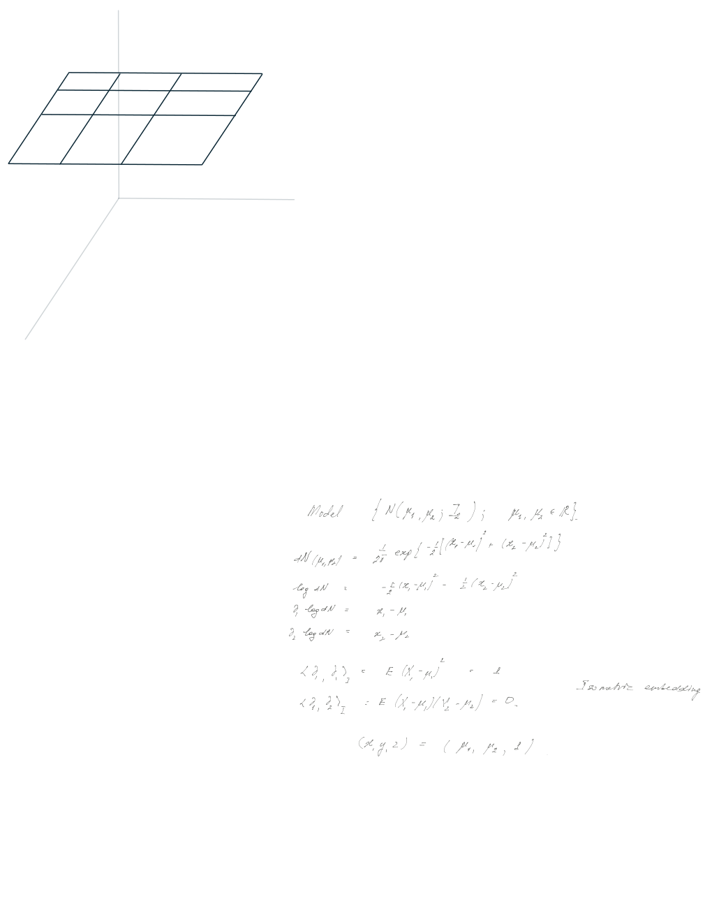
*