Thin Position through the lens of trisections of 4-manifolds
Abstract
Motivated by M. Scharlemann and A. Thompson’s definition of thin position of 3-manifolds, we define the width of a handle decomposition a 4-manifold and introduce the notion of thin position of a compact smooth 4-manifold. We determine all manifolds having width equal to , and give a relation between the width of and its double . In particular, we describe how to obtain genus and trisection diagrams for sphere bundles over orientable and non-orientable surfaces of genus , respectively. By last, we study the problem of describing relative handlebodies as cyclic covers of 4-space branched along knotted surfaces from the width perspective.
keywords
Heegaard Splittings, Kirby diagrams, Thin position, Trisections of four manifolds1 Introduction
In 1994, M. Scharlemann and A. Thompson introduced the notion of thin position of 3-manifolds. In their work [16], they described thin position as follows:
“Any closed orientable 3-manifold can be constructed as follows: begin with some 0-handles, add some 1-handles, then some 2-handles, then some more 1-handles, etc… and conclude by adding some 3-handles. Of course can be built less elaborately: in the previous description, all the 1-handles can be added at once, followed by all the 2-handles. This corresponds to a Heegaard splitting of the manifold; the 0- and 1-handles comprise one handlebody of the Heegaard splitting, the 2- and 3-handles to the other. The idea of thin position is to build the manifold as first described, with a succession of 1-handles and 2-handles chosen to keep the boundaries of the intermediate steps as simple as possible.”
The complexity that the position of Scharlemann and Thompson seeks to minimize is the width of a handle decomposition of a 3-manifold. It is in terms of the genera of the surfaces between the 1- and 2-handles.
In dimension four, we can apply a similar reasoning to talk about thin position of a closed 4-manifold if we add the necessary 4-handles at the end of the process. In this context, the action of alternating between 1-, 2- and 3-handles becomes a suitable decomposition of a handle decomposition and the question now is what do we want “as simple as possible” to mean.
In 2013, D. Gay and R. Kirby [7] showed that every closed smooth 4-manifold admits a trisection. A trisection of a closed 4-manifold is a decomposition of into three 4-dimensional 1-handlebodies with pairwise intersection being a connected 3-dimensional handlebody and triple intersection a connected closed surface. In [7] and [9], a correspondance between trisections and certain handle decompositions was described. In such decompositions, all the 1-handles are added at once, followed by all the 2-handles and all the 3-handles. The 0- and 1-handles comprise the first 1-handlebody of the trisection, the 3- and 4-handles form the second 1-handlebody, and the third 1-handlebody is given by a suitable neighborhood of the 2-handles. With this in mind, one can think of trisections as the 4-dimensional analogue of Heegaard splittings of with the “trisection surface” being the triple intersection of the 4-dimensional 1-handlebodies.
In this paper, we use ideas of trisections of 4-manifolds from [9] to define the width of a handle decomposition of a connected 4-manifold. This allows us to define the width of a 4-manifold by looking at the minimum width among all possible handle decompositions of . Similar to [16], the width of is a multiset where is a function of some “trisection-like surfaces” for the attaching link of the 2-handles of (see Section 3.1 for the detailed definition).
In Section 3, we describe situations when the width is not minimal. The interested reader should compare these situations with the rules to decrease the width introduced in [16]. We also determine all 4-manifolds satisfying . We show
Theorem 3.11.
Let be a connected 4-manifold satisfying . Then is diffeomorphic to a (boundary) connected sum of copies of , , and linear plumbings of disk bundles over the sphere.
In Section 4, we define the notion of the nerve of a 4-manifold obtained by adding 2-handles to along , basically the same as the nerve of a trisection for a closed 4-manifold. In Subsection 4.2, we show how the nerves of the suitable relative handlebodies around the 2-handles carry the width information of the handle decomposition.We use this to show that the operation of turning a handle decomposition up-side-down leaves the width invariant. We also prove
Proposition 4.8.
Let and be connected 4-manifolds with non-empty boundary. Suppose is a diffeomorphism between their boundaries. Then
In Subsection 4.3, we explain how handle decompositions of closed 4-manifolds of width equal to a single element correspond to trisections of 4-manifolds. This allows us to specialize some of our results to the theory of trisections of 4-manifolds (see Example 4.11 and Section 5.1.2).
In Example 4.11, we give an upper bound for the width of sphere bundles over closed surfaces. In particular, we are able to obtain low genus trisection diagrams for such manifolds. Denote by , the disk bundles of euler number over an orientable and non-orientable surface of genus , respectively. We describe how to obtain trisection diagrams of genus and for and , respectively (see Example 4.11). It is important to mention that trisection diagrams for such manifolds have been described before in [7] and [5]. But the existance of lower genus diagrams was proven in [2] with no explicit drawings. In Figure 4, we draw explicit lower genus diagrams for and .
In Section 5, we study the problem of describing relative handlebodies as cyclic covers of 4-space branched along knotted surfaces from the width perspective. We use ideas from [10], [11] and [12] to prove
Theorem 5.10.
Let be a closed 4-manifold. Then is the -fold cyclic cover of branched along a knotted surface if and only if admits a -symmetric trisection diagram.
In [16], M. Scharlemann and A. Thompson proved that 3-manifolds of are 2-fold branched covers of connected sums of . Subsection 5.2 is a digression on an attempt of lifting this result to 4-manifolds with connected boundary.
Acknowledgements. The author would like to thank the Topology group of the University of Iowa for listening and commenting on previous versions of this work. Special thanks to Maggy Tomova, Charles Frohman and Mitchell Messmore.
2 Preliminaries
Along this work, all manifolds will be compact, smooth, oriented and connected unless the opposite is stated. For an embedded submanifold of any dimension, will denote the closed tubular neigborhood of in .
For , an -dimensional -handle is a copy of , attached to the boundary of an -manifold along by an embedding . By definition, 0-handles are attached along the empty set. In dimension 3, 1-handles are attached along pairs of disjoint disks, 2-handles along annuli, and 3-handles along 2-spheres. In dimension 4, 1-handles are attached along pairs of disjoint 3-balls, 2-handles along solid tori (hence framed knots), 3-handles along thickened 2-spheres, and 4-handles along copies of in .
A handle decomposition of (relative to ) is an identification of with a manifold obtained from by attaching handles along . We will usually start building with thus start by adding some 0-handles. The action on of a -handle addition is by surgery on . In other words, the new boundary is given by . For a more detailed review of the calculus on handlebody diagrams, Chapter 1 of [1] or Chapters 4 and 5 of [8] are good references.
The 4-manifold obtained by attaching a handle to the 4-manifold will be denoted by . If , we will write to denote the surgered 3-manifold . If is a framed link in , will denote the surgered manifold. For simplicity, a 1-handlebody will mean a 4-ball with some 4-dimensional 1-handles attached and the three dimensional analugue will be called just handlebody.
A Heegaard splitting of a closed 3-manifold is a decomposition of in two handlebodies with common part a connected surface of genus . The smallest such is the Heegaard genus of , .
A trisection of a closed 4-manifold is a decomposition of in three 1-handlebodies so that the double intersections are connected 3-dimensional handlebodies, ; and the triple intersection is a closed connected surface of genus , . It follows from the definitions that is a Heegaard splitting for the boundary of , which is homeomorphic to the connected sum of some copies of . The triplet is called the nerve of the trisection.
Let be a link in a connected closed 3-manifold. Denote by the smallest number of embedded arcs with such that is a handlebody. is called the tunnel number of in and is a system of tunnels for . Note that the surface induces a Heegaard splitting of with . Define to be the smallest genus of a Heegaard surface for with being a subset of the core of one of the handlebodies. We have
The equation above will serve to us as an equivalent definition of tunnel number. If , define . We will need the following computation of the tunnel number of split links.
Lemma 2.1.
Let , be links inside closed three-manifolds , , respectively. Let and . Then
Furthermore, if and , then
Proof.
We will prove the equation for , the other case is similar. One can see that the LHS is smaller by constructing a system of tunnels of cardinality .
We now prove . Let be a system of tunnels for in with , and let , , . By construction, is a Heegaard splitting of genus for with a handlebody and a compression body with inner boundary the collection of tori given by . An application of Haken’s Lemma gives us the existance of a sphere intersecting in one simple closed loop, separating in and , here denotes minus an open 3-ball. In other words, is the connected sum of Heegaard splittings for and , say for , satisfying that is a compression body with inner boundary the tori . But recall that a compression body deformation retracts to the wedge of its inner boundary with a finite collection of arcs in the interior of the compression body with endpoints on the inner boundary. Thus is the tubular neighborhood of the union of with a collection of arcs with endpoints on . This shows that . By last, notice that and, since , we get
Hence, . ∎
3 The width of a Kirby diagram
In the following section, we define the notion of the width of a handle decomposition of a 4-manifold and the width of a 4-manifold. Following [16] closely, we describe specific cases when the width of a decomposition is not minimal and classify 4-manifolds with low width.
3.1 Definition of width
Let be a connected, compact, smooth 4-manifold. Consider a handle decomposition of
where , , , , are collections of 0-handles, 1-handles, 2-handles, 3-handles and 4-handles, respectively. We are thinking of building in steps; starting with , then adding , then , then , etc.
For each , denote by and let be the cores of the attaching regions of the 2-handles . Note that might be disconnected and that is a link (possibly empty) in each component of . For a connected component of , set . If is not empty, define ; if define where is the Heegaard genus of . Define
Definition 3.1.
The width of the handle decomposition is the multiset . The width of is the infimum of all widths among all possible handle decompositions of . The infimum is taken with respect to the following order:
Let and be two bounded multisets of ordered in a decreasing way. Then if and only if there is an index such that for and .
We say that is in thin position if there is with minimal . It is important to mention that the infimum is always achieved; so for smooth compact manifolds the width always exists. For completeness, we include a proof of this fact in Lemma 3.3.
Remark 3.2.
The decomposition has empty width so . For non-empty diagrams, the width will be a finite multiset of odd integers .
Lemma 3.3.
Let be the set of all sequences of non-negative integers with finitely many non-zero elements endowed with the order described above. Then any non-empty set has a minimal element.
Proof.
Let be non-empty. For an element , we define to be the th largest element in P. Take and define the set . Since we can consider and . We inductively define the sets , and . By definition, the sequence is decreasing in , so it is stationary; say for all . Let . By construction for all . For we have the following inequalities,
Thus for all . But , so all but finitely many components are non-zero. Hence and . ∎
3.2 Ways to decrease the width
Proposition 3.4.
Let be a thin position of . For every , define .
- 1.
Suppose that for some , one of the level 3-manifolds , , or is diffeomorphic to , say X. Then has no components diffeomorphic to unless one of them is equal to or .
- 2.
If for some , then .
- 3.
If for some , then .
Proof.
- 1.
We will prove the case , the other cases are similar. Within this case, we have two options. If , we can remove the handles to reduce the width. If , we can remove the handles to reduce the width.
- 2.
Suppose for some . We will show that and are both non-empty. Suppose first . In particular, . If we consider the new decomposition of by merging (taking the union of) and we will get the multiset , which has lower width, a contradiction. In a similar fashion, suppose that is empty: By defining to be , we obtain a new decomposition of with width being the multiset , which is smaller, contradicting the minimality of the width.
We have shown that if , then and are both non-empty. Notice that . Thus if we take the new decomposition given by merging and , then the complexity will not change. The width of this new decomposition will be the original width without the element , which is strictly lower.
Therefore, has to be non-empty if .
- 3.
The result follows by turning up-side-down and applying Part 2 of this proposition (see Lemma 4.7).
∎
We say that a link in a 3-manifold splits if there exists a separating sphere disjoint from . In such case, we can decompose , with and links in the corresponding pieces, . The following proposition studies how the width could change if one of the attaching links of the 2-handles splits in .
Proposition 3.5.
Let be a handle decomposition for . Suppose that there is a component so that the link splits in . Write , and let be the 2-handles with attaching region .
Consider the new handle decomposition of obtained from by separating the 2-handles of , adding first and then .
- 1.
If or , then
- 2.
If and , then
Proof.
The following lemma states that the width of a decomposition is invariant under certain types of sliding. More precisely, if we slide handles on latter levels along previous handles, the width does not change. It follows that if a level is a pair of cancelling handles, we can remove such handles from the decomposition, decreasing the width.
Lemma 3.6.
Let be a handle decomposition of . For fixed , take connected components and and let be a decomposition obtained by sliding along . Then and have the same width.
Proof.
In terms of the attaching regions of the handles, sliding along corresponds to an isotopy of the attaching circles of in , which does not affect the values of . Hence the width does not change. ∎
Lemma 3.7.
If is a thin position of , then does not contain a pair of cancelling 1-handle and 2-handle say, where is the attaching region of a handle of and , so that is unlinked with and goes through geometrically once.
Similarly, does not contain a pair of cancelling 2-handle and 3-handle where the attaching region of is disjoint from .
Proof.
We prove the contrapositive. Suppose that there is a 1/2-cancelling pair , such that is disjoint from . In order to erase the pair from the diagram, we need to slide along the other handles of intersecting . By assumption such handles can only be part of (), so we can slide them along without changing and then erase the pair , reducing the width. The case for 2/3-cancelling pairs is similar. It also follows from the fact that (see Lemma 4.7), where is the up-side-down handle decomposition of . ∎
3.3 Manifolds with small width
By taking the simplest handle decompositions of and , we see that these manifolds have width equal to . We will now show that no other manifold has such width. We also study the equation
For a handle decomposition , denote by
Proposition 3.8.
Let be a closed 4-manifold satisfying . Then is diffeomorphic to either or .
Proof.
Let be a decomposition for of width equal to , we can assume . Suppose first , then is not empty and the Heegaard genus of is since . Thus and admits a handle decomposition with only one handle, i.e. .
Suppose now that . We have that , so and . It follows that , giving us two options. If , then and is an unknot with framing say . Recall that is closed so must be a connected sum of . This forces to be or , which implies that is either or .
Assume the second case: and . Since , a neighborhood of induces a genus one Heegaard splitting of . Uniqueness of such splittings [4] implies that intersects geometrically once and that is a cancelling pair for . In particular we conclude . ∎
Proposition 3.9.
Let be a connected 4-manifold and let be a thin position of satisfying . Suppose that the level 3-manifolds are connected for all . Then is diffeomorphic to a (boundary) connected sum of copies of , , and linear plumbings of disk bundles over the sphere.
Proof.
By definition of , the condition implies and for all . Since is a lens space and is connected, we get . Note that if and only if and . Thus and either or where and are collections of at most ones. Thus we can assume that .
In a similar vein, implies , and if and only if , giving us a decomposition as above. Thus we may assume that for all . Moreover, if both and are non-empty, then which forces . So is isotopic to . Then is a cancelling pair, contradicting the minimality of the width by Lemma 3.7. Thus by avoiding the case , we may assume that .
As before note that ; in particular, is an knot for all . Since , is a unknot with framing . is a lens space , with . Decompose as where and is a solid torus so that the push-off of with framing bounds a meridian disk in . Since , we get and, by uniqueness of genus one Heegaard splittings for lens spaces [4], we conclude that is isotopic (in ) to the core of or .
Suppose is isotopic to the core of . Let be an orientation reversing homeomorphism mapping the meridian of , say , to the curve with framing on in . Let be the meridian and preferred longitude of induced by , is the boundary of the meridian of . By construction, . We can take and a longitude of so that in the ordered basis , is given by the matrix . We make such choice since the map is determined up to isotopy by . In particular, is isotopic in to and so it can be pushed into , becoming parallel to . Hence we can assume that is isotopic to the core of . Then is a Hopf link with framings say .
For , is a genus one Heegaard surface for . We can decompose the lens space as the union , where is the solid torus such that the push-off of with framing bounds a meridian disk in and . has tunnel number one so uniqueness of genus one Heegaard splittings for lens spaces [4] forces to be isotopic in to the core of either or . Without loss of generality, . Using an argument analogous to that given above, we can pick an adequate attaching map so that we can isotope out of so that is parallel to a meridian of in . Let be the solid torus with meridian disk a curve in and framing . If we sit in the core of , it is clear that and induce a Heegaard splitting for (note that is a product region ).
We have shown that we can perturb (without changing the width) so that are isotopic to the link in Figure 1. Also, notice that if () is the solid torus apearing in after surgering along , then is a product region. We can proceed inductively, repeating the argument above to conclude that is the Kirby diagram of a “linear” plumbing of disk bundles over spheres.

∎
Corollary 3.10.
For closed prime 4-manifolds, if and only if .
Theorem 3.11.
Let be a connected 4-manifold satisfying . Then is diffeomorphic to a (boundary) connected sum of copies of , , and linear plumbings of disk bundles over the sphere.
Proof.
Let be a thin position of of width . The level 3-manifolds , and may not be connected. By definition, where the sum runs through all connected components of and . In particular, and for all . Let be the unique component of such that .
Suppose that , where are some connected components. Note that for all . Suppose that , then . So there is a 1-handle so that is a 1/2-cancelling pair. Lemma 3.7 contradicts the minimality of the width. We have shown that whenever , the 1-handles of only act as connected sums of distinct components of . In other words, does not intersect the attaching regions of the 1-handles of . Moreover, since and whenever , it must be the case that is an unknot in which we can isotope in (and so slide over previous handles) to be away from the attaching regions of in .
By turning up-side-down, the same argument shows that if , then the attaching sphere of each 3-handle is separating in . In particular, since , the attaching sphere of must bound a 3-ball in . We can then isotope these attaching spheres in (thus slide over previous handles) so that are disjoint from in .
We will prove the theorem by induction on the number of 2-handles of . If has no 2-handles the result is clear. Suppose then it has at least one 2-handle. Pick to be the smallest index with , then . is an unknot in so it can be isotoped to lie inside a 3-ball bounded by a 2-sphere disjoint from the attaching region of the previous handles in . Suppose , then for some connected components . By the previous paragraph, and can be picked to avoid the attaching spheres of . We can then think of and as embedded in and so in ; one can do this by flowing and using the morse map induced by . If lies in the same component as , then we can isotope in to lie inside . To see this, recall that where all but (at most) one are equal to , and the non- component must contain . Such isotopies correspond to handle slides of over previous handles which keep the width unchanged. As before, and can be picked to be disjoint from the attaching regions of .
We can continue this process of isotopying to be inside until either for some or lies in a different component of than the one containing . In any case, this implies that the component of containing must be . Focusing our attention on the attaching region of the handles in , the sphere will separate the attaching links from the rest of the Kirby diagram for . This shows that splits as a connected sum where has a handle decomposition given by . Notice here that , , satisfies the conditions of Proposition 3.9, and has strictly less 2-handles than . This concludes the inductive step. ∎
4 Relative handlebodies and generalized trisections
In dimension 3, thin position arguments reduce the problem to the study properties of compression bodies. In dimension 4, we will break our thinned 4-manifold in pieces that only contain the information of the 2-handles: the relative handlebodies . In Subsection 4.1, we will see two ways of representing these relative handlebodies. Similar versions of the content of this subsection can be found in [9] and [7]. We include the details here due to the slight change of setting. We will use the above in Subsection 4.2 to show that the width does not change when turning up-side-down a handle decomposition. In Subsection 4.3 we will relate the width with trisections of closed 4-manifolds. As an application, in Subsection 4.4 we give an upper bound for the width of the union of two 4-manifolds, which we use to compute an upper bound for the width of sphere bundles over connected surfaces.
4.1 Nerves of relative handlebodies
We will describe a way to decompose 4-manifolds obtained by 2-handle attachements on collars of closed 3-manifolds. The ideas in this subsection are motivated by the notion of a Heegaard-Kirby diagrams introduced in [9]. It would be interesting to see what one can say about thinned manifolds using results from dimension three and lemmas 4.1 and 4.3. The interested reader can look at the proofs of Proposition 3.5 and Theorem 1.2 of [9] to see examples of this technique.
For a closed surface and a collection of pairwise disjoint simple closed curves , denote by the closed surface resulting from compressing along . In other words, is obtained by capping-off with 2-disks the boundary components of .
Let be a closed surface of genus and let be three collections of pairwise disjoint non-separating simple closed curves determining three handlebodies , and , respectively. Suppose that is a Heegaard splitting for , . We build a 4-manifold as follows: Attach 2-handles to along and with framings induced by . The resulting 4-manifold, denoted by , has three special 2-spheres on its connected boundary: , and . Attach one 3-handle along each sphere to obtain a 4-manifold, denoted by , with three boundary components diffeomorphic to: , and . Let be the result of capping-off with 3- and 4-handles the boundary component of . A schematic picture of can be found on the right side of Figure 2.
Lemma 4.1.
is determined by the embedding of .
Proof.
The procedure of capping-off the boundary component of given by with 3- and 4-handles is unique by [6], so it is enough to show that is determined by the associated handlebodies , and . Recall that two collections of pairwise disjoint non-separating simple closed curves in determine the same handlebody if and only if they differ by disk slides on the surface. Thus by the symmetry of the construction of , it suffices to check when and differ by one disk slide. In this setup, disk slides correspond to 4-dimensional 2-handle slides so .
Label the components of and so that and for all . It follows that and are disjoint, forcing to be disconnected. Let and be its two components and label them so that is a thrice punctured sphere with for some . Write the corresponding components of as . Let be the 4-manifold resulting from by attaching a 2-handle along and 3-handles along , and .
Let be the 2-handle attached along and the 3-handle attached along , for . Since the framing of is given by , one can check that the intersection when written in the coordinates of the handle. Also, the belt sphere of , which is given by , is isotopic in to a loop of the form for some . To see that, recall that the belt sphere is a component of the Hopf link in . It follows that the belt sphere of intersects in two points, one per side of in . Thus the belt sphere intersects in one point. On the other hand, is the union of with the cores of the 2-handles given by , and , which are disjoint from the belt sphere of . Hence the belt sphere of will intersect geometrically once. Thus the 3-handle cancels with . Similarly, intersects the belt of once. In order to eliminate and , it is necessary to slide along ; this will change the attaching sphere of from to . Therefore, . Analogously, one can show that , and so only depends on the handlebodies . ∎
Definition 4.2.
Let be three connected handlebodies with common boundary a surface . We say that the tuple is a nerve of W if for some collections of curves determining , respectively.
Let be a framed link inside a closed 3-manifold , and let be the smooth 4-manifold built from by attaching 2-handles along .
There is a correspondance between 4-manifolds of the form and . For the closed case, is a trisection diagram (see Subsection 4.3), and the correspondance has been proven in [7]. The proofs can be extended to our context.
The following lemma is essentially Lemma 4.1 of [11] or Lemma 14 of [7]. For completeness and due to the slight change of setting (closed case vs relative case), we include a proof.
Lemma 4.3.
Let be a framed link inside a closed 3-manifold. Then there exist handllebodies , , so that .
Proof.
Take a Heegaard splitting of genus of so that is a subset of its core; i.e. is an admissible pair. Then after surgery along is still a 3-dimensional handlebody denoted by . Let be a Morse function arising from the construction of with , , and all critical points of index 2 at . The flow of restricted to induces an injective isotopy in between and the handlebody , thus a product region. We can use the latter region to add a copy of to and assume the three handlebodies to intersect simultaneously at the surface (see Figure 2). By construction, is a Heegaard splitting for a connected sum of copies of .
Let be the 4-manifold given by flowing with . is obtained by adding 2-handles to along . Note that is a 4-dimensional 1-handlebody of genus with one 0-handle and 1-handles, where the handles are in correspondance with any set of meridians determining . Since is a subset of the core of , 2-handles along cancel 1-handles of . Hence is a 1-handlebody of genus . It follows that . ∎

Lemma 4.4.
Let be a surface and be handlebodies with boundary satisfying for some . Then for , there is a link satisfying .
Proof.
Since , there are collections of curves determining and , respectively, such that , for all and , for all . The desired link is given by . Notice that the curves, which induce , are useful to determine the embedding of into and so the embedding of . ∎
Remark 4.5.
Notice that if , then , and is a nerve for for any Heegaard splitting of . In particular, is a nerve for .
Remark 4.6.
We can build an up-side-down version of from by attaching 2-handles to along , where are co-cores of the 2-handles along . In terms of nerves, one can see that if , then this up-side-down presentation for can be described by .
4.2 Relative handlebodies and width
Let be a handle decomposition of . Recall that
For each , denote by , note that may be disconnected. Let be nerves for with smallest genus11 1 For closed disconnected surfaces, the genus is the sum of the genera of the connected components. satisfying . can be decomposed as
Note that the proofs of Lemmas 4.3 and 4.4 show that
Let be the up-side-down handle decomposition of , where , , , and . The relative handlebodies satisfy (see Remark 4.6),
We have proven the following
Lemma 4.7.
Let be a handle decomposition of . Then
4.3 Relative handlebodies and trisections of 4-manifolds
An interesting case of the discussion in Subsection 4.2 is when is closed and the handle decomposition is self-indexed; i.e., . Here, the decomposition in relative handlebodies becomes
where , , is the attaching region of the 2-handles and is the cobordism between and (see Figure 2).
Note that the last expression is a trisection of . Hence, , where is the smallest genus trisection surface for inducing the handle decomposition .
One would expect closed 4-manifolds with being a singleton to be “small”. For example, Proposition 3.8 implies that the only 4-manifolds of trisection genus one are and .
For a generic handle decomposition of , we can think of a generalized trisection to be the collection of nerves for the relative handlebodies , together with data describing the 1-handles and 3-handles pasting them along some boundary components. With this philosophy in mind, in some part of the rest of this work we will derive results about trisections of 4-manifolds as a particular case of constructions on thin position (see Example 4.11 and Section 5.1.2).
4.4 Width under specific operations
Let be a 4-manifold with non-empty boundary and denote by the double of ; i.e. . If is connected, a Kirby diagram for the double of can be built by adding an unknotted 2-handle with framming zero around each 2-handle of a Kirby diagram for . Let be a self-indexed handle decomposition in thin position for with no 3-handles. Denote by the attaching links of the new 2-handles for . An application of the slam-dunk move [8], shows that the components of the link are isotopic in to the cores of the solid tori after surgery along . Thus the tunnel number of in is the same as the tunnel number of in . In particular, .
We can refine the above argument as follows.
Proposition 4.8.
Let and be connected 4-manifolds with non-empty boundary. Suppose is a diffeomorphism between their boundaries. Then
Proof.
Let and be a thin position for and , respectively, and consider a decomposition of given by doing first, followed by in the opposite order. By construction,
The result follows from Lemma 4.7. ∎
Corollary 4.9.
Let be a 4-manifold with non-empty boundary. Then
Remark 4.10.
It is important to mention that if one decides to add the 2-handles after (or at the same time), the tunnel number of in will be equal to the tunnel number of in ; allowing the complexity to change with no control. Hence, the upper bound on Corollary 4.9 is expected to be sharp only for special cases.
Example 4.11 (Sphere bundles over surfaces).
Let , and denote by , the orientable and non-orientable surface of genus , respectively. Let be the disk bundles over and with Euler number , respectively. Kirby diagrams for and with only one 2-handle are known (Fig. 3), so stimates for the width of such 4-manifolds can be found. More explicitly, for , and . Using Proposition 4.9, we obtain estimates for the width of the corresponding doubles; i.e. sphere bundles over surfaces.
For this particular examples, one can add all 2-handles of (resp. ) at the same time and get tunnel numbers (resp. ). Lemma 4.3 together with the discussion on Subsection 4.3 imply that, to draw a genus trisection surface for , it is enough to find a system of tunnels for the attaching region of the 2-handles22 2 This is Lemma 2.3 of [12].. Thus we can draw diagrams for (resp. ) of genus (resp. ). For completeness, we draw the diagrams for genus 1 case in Figure 4.


5 Symmetries of relative handlebodies
In [16], M. Scharlemann and A. Thompson proved that 3-manifolds of are 2-fold branched covers of connected sums of copies of . In this section, we relate ideas of trisections of 4-manifolds from [9], [10] and [12] to discuss an attempt of lifting this result to 4-manifolds with connected boundary. In Subsection 5.1 we study symmetries on the relative handlebodies . We use this in Subsection 5.1.2 to talk about symmetric trisection diagrams and to prove a “trisected version” of a Theorem of J. Birman and H. Hilden. In Subsection 5.2 we study the extension problem: how to paste symmetric pieces of .
5.1 Symmetric nerves
In this subsection will denote a 4-manifold of the form for some link .
Definition 5.1.
We say that a nerve for is p-symmetric if there is a piecewise-linear homeomorphism of finite period , extending to the interior of each handlebody, satisfying
- 1.
For each handlebody, the orbit space by the action of is a 3-ball.
- 2.
for all .
- 3.
The image of the fix set of on each handlebody is an unknotted set of arcs in the quotient.
Remark 5.2.
The 2-symmetric condition of a nerve is equivalent to the existance of an involution of extending to the interior of each handlebody such that is conjugate to the hyperelliptic involution.
Using the ideas of [10], one can show that if is a -symmetric nerve of , then the finite order map extends to .
Proposition 5.3.
Let be a framed link inside a closed 3-manifold and let be a nerve for . If is -symmetric, then is a -fold cyclic covering of branched along a properly embedded knotted surface with boundary in both .
Proof.
By fixing a model handlebody of genus , we can assume are standard and take maps between the corresponding boundaries codifying the pairwise intersections. Let be the order homeomorphism of extending to the three handlebodies. By assumption, commutes with the -maps and hence the maps descend to the quotients , , (Figure 5).
By definition the quotient map on each handlebody is a -fold cyclic branched cover of along a collection of boundary parallel arcs in , say , and .
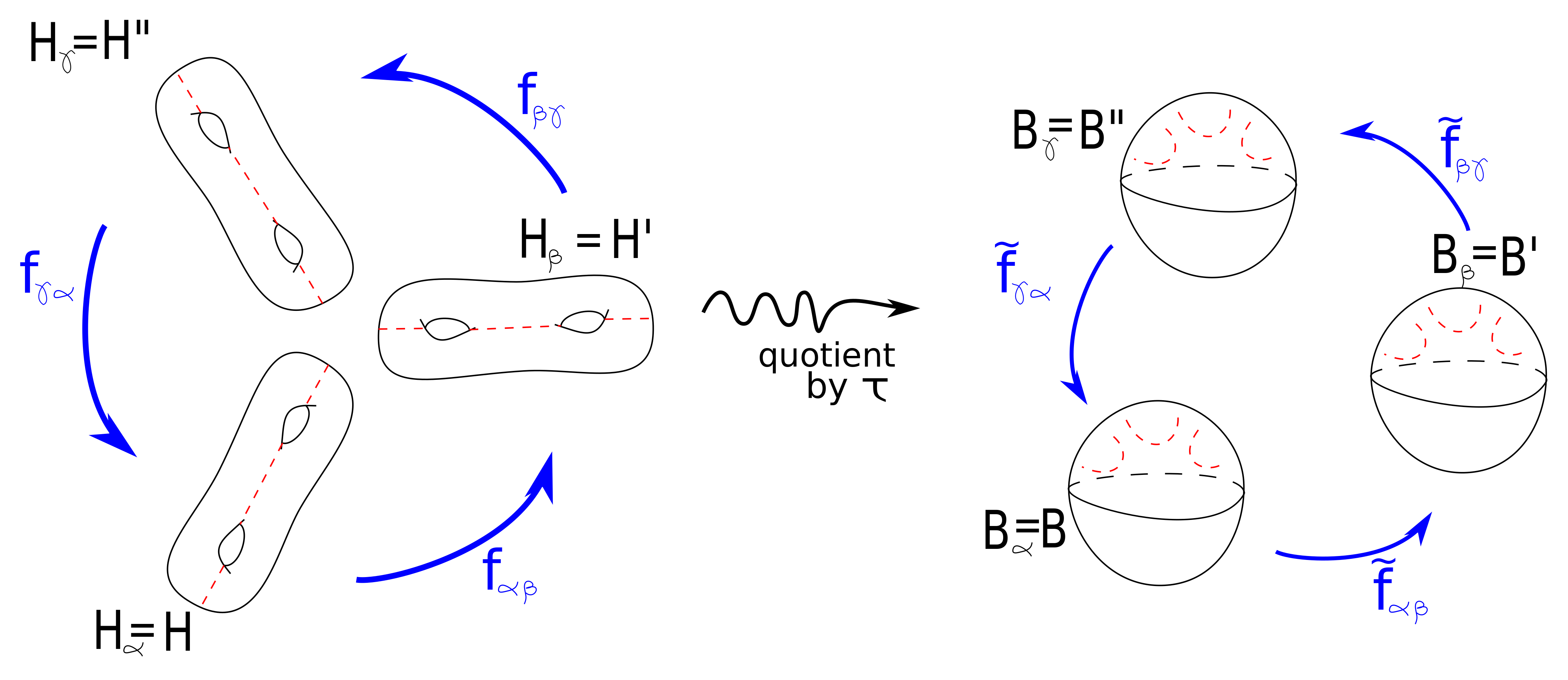
Since, is a subset of the core of , each component of is dual to a meridian disk of , and the 3-manifold is a connected sum of copies of . A corollary in Section 2 of [15] states that such 3-manifolds arise as fold cyclic branched cover of only when the branched set is an unlink. Thus is an unlink in , which bounds a unique collection of trivial disks in by Lemma 2.3 of [11]. By Remark 4.5, the tuple is a nerve for , and one can complete to a properly embedded surface by attaching the collection along . By construction,
We can now take the -fold cyclic covering of branched along and lift the nerve of to a nerve for the resulting 4-manifold. Recall that the -fold cyclic cover of a 4-ball branched along a collection of trivial disks is also 4-dimensional 1-handlebody. By construction, the new tuple is indeed equal to the original nerve for . Lemma 4.1 concludes that is the -fold cyclic branched covering of along and that the map extends to all . ∎
Remark 5.4.
Suppose that a -symmetric nerve comes from a Kirby diagram with 1-handles and 2-handles , that is, and where is a system of tunnels for the attaching link of the 2-handles in . Since , we can use the argument in Proposition 5.3 to obtain a action on which provides a description of as a -fold cyclic cover of branched along a properly embedded knotted surface.
Remark 5.5.
Although Section 5 was written mainly to discuss the symmetries of 4-manifolds of width less than (see Section 5.2.1), one can talk about constructions of more general 4-manifolds than those that appear in Definition 4.2. Take a closed orientable surface ; pick finitely many points and meridian systems for handlebodies . Let be the 4-manifold obtained by attaching 2-handles to along for and capping off with 3- and 4-handles (if desired) some boundary components corresponding to Heegaard splittings of connected sums of copies of . The tuple will be the nerve of and Proposition 5.3 will immediately extend to this context using the same proof. One can naively ask if every 4-manifold with disconnected boundary admits such decomposition.
Proposition 5.6.
Let and let be as in Remark 5.5. If is -symmetric, then is the -fold cover of with 4-balls removed branched along a properly embedded surface.
5.1.1 Drawing the branched set
We will briefly describe how to obtain band diagrams for the branched set of a given -symmetric nerve. Recall the notation of Proposition 5.3 (see Fig. 5 for simplicity). In Lemma 3.3 of [10], J. Meier and A. Zupan described an algorithm to obtain a banded link diagram (also called movie presentation) for from the tuple , which the authors called a bridge trisection diagram for . Using our current notation, the algorithm goes as follows:
Lemma 5.7 (Lemma 3.3 of [10] rephrased).
Let be a nerve for and let be three collections of trivial arcs on with the same set of end points in such that is an unlink in . Let be a collection of shadows of , and excise one arc of corresponding to each component of . Denote by the remaining shadows and let . Then is a banded diagram for in .
The bands of correspond to saddles of ocurring inside the collection of disks that bounds in the 4-ball. One can change, if desired, the roles of and in the statement of Lemma 5.7 to get the “reversed” banded diagram for .
Example 5.8.
Figure 7 exemplifies the procedure of Proposition 5.3 to obtain a movie presentation for the branching surface in the case that admits a symmetric nerve. This breaks in four steps as follows:
- 1.
Find a system of tunnels for in so that the corresponding nerve is -symmetric.
- 2.
Draw three collections of non-separating curves in determining the handlebodies , , .
- 3.
Project the curves with the finite order map to obtain the tuple .
- 4.
Apply the algorithm described in Lemma 5.7 to draw the banded diagram for .


5.1.2 An application to trisections of 4-manifolds
We finish this subsection with an application of Proposition 5.3 to the theory of trisections of closed 4-manifolds. We will show that 4-manifolds with symmetric trisections are 2-fold covers of branched along knotted surfaces. It is important to mention that subsections 5.2 and 5.2.1 are independent of the following.
In [3], J. Birman and H. Hilden studied the relations between ‘‘p-symmetric” Heegaard splittings and branched covering representations of closed 3-manifolds. For example, they showed33 3 This is Theorem 1 of [3]. that every genus Heegaard splitting of a closed 3-manifold may be represented as a -sheeted branched covering of , with branching set a 1-manifold of at most components.
Question 5.9.
We can partially answer Question 5.9 in Theorem 5.10. The interested reader can compare this theorem in the case of with Corollary 11.3 of [1] or with Theorem 3 of [14]. One can think of this result as a trisection analogue of Theorems 2-5 in [3].
Theorem 5.10.
Let be a closed 4-manifold. Then is the -fold cyclic cover of branched along a knotted surface if and only if admits a -symmetric trisection diagram.
Proof.
The forward direction was discussed in Section 2.6 of [10]. For the backwards direction, recall that in a trisection the triplet has the property that the 3-manifolds , and are homeomorphic to connected sums of copies of . Thus for each pair, we can use the argument in Proposition 5.3 to extend the involution to all . ∎
5.2 Extending involutions
Let be a handle decomposition decomposition of a smooth manifold . Denote by , , , and . is obtained by attaching 2-handles to along , so let be a nerve for with . By construction, is divided in two parts: and . Suppose each is 2-symmetric. By Proposition 5.3, there are involutions with fixed set a properly embedded surface . By construction, and are induced by involutions on the handlebodies .
In , and cobound a submanifold given by adding 3-handles and 1-handles to along . We are interested in knowing under what conditions the involution on the pair can be extended to the interior of such cobordism, obtaining involutions on bigger pieces of . With the setting just described, we can extend the involution when adding 1-handles.
Lemma 5.11.
Let be an involution of a closed 3-manifold (possibly disconnected) with 1-dimensional fixed set and let be the 4-manifolds obtained from by adding a 1-handle along . Then there is an involution of so that . Furthermore, is diffeomorphic to with a 1-handle attached.
Proof.
Write where has coordinates . Consider given by . The map models a 4-dimensional 1-handle attachement. Define by . is an involution of satisfying for all . Notice that is again a 4-ball, and the quotient map is a 2-fold cover of branched along the 2-disk
is given by which models a 2-dimensional 1-handle attachement. Take to be two disjoint closed 3-balls so that is one arc. Pick coordinates for so that and . By hypothesis, where
By construction, and agree on a neigborhood of . We then obtain the desired involution in . ∎
Remark 5.12.
Let be the new boundary component of ; we have . Furthermore, one can check that
Thus the action of before and after the 1-handle attachment in Lemma 5.11 is described by Figure 8. In particular, if and are neigborhoods of points of the intersection where is a Heegaard surface fixed setwise by , then the involution will delete the corresponding intersection points between and the new Heegaard surface.

5.2.1 When the width is less than {5}
In [16], M. Scharlemann and A. Thompson showed that if the width of a 3-manifold is less than {5}, then it is a 2-fold branched cover of a connected sum of copies of . In the following subsection, we will apply the previous discussion to describe an attempt of proving the analogue of this result in dimension four, say: if is a 4-manifold with , then is the 2-fold cover of connected sum of copies of with 4-balls removed, branched along a properly embedded surface.
The outline of the solution is analogous to the original one in [16]: we first show that the blocks are branched covers of copies of and then we study how to paste them together preserving the branched covering map. In dimension three this pasting problem resulted being a known mapping class group problem. From the 3-manifold theory perspective, it is interesting how this attempt reduces a 4-dimensional problem to the study of non-uniqueness of genus two Heegaard splittings of closed 3-manifolds.
Proposition 5.13.
If , each admits a smooth involution such that the projection map , is a 2-fold cover of branched along a properly embedded surface . Furthermore, for , we can take the involution to be defined on and , respectively.
Proof.
Recall that is obtained by attaching 2-handles to along . Since , which gives us the existance of a Heegaard splitting of of genus at most 2 such that . Then, is a nerve for by Lemma 4.3. The hyperelliptic involution on fixes the isotopy class of unoriented curves in , so it extends to the interior of , and ; thus is 2-symmetric for every . The result follows from Proposition 5.3.
When , is a Heegaard splitting for . By uniqueness of involutions on such manifolds, we will obtain that is also an unlink in , thus we can cap off with 3- and 4-handles on that side and extend the surface (with its involution) with the unique boundary parallel disks; obtaining a branched cover . We proceed analugously for . ∎
We now proceed to describe how to paste the blocks preserving their involutions. Since , we have that and for every connected component and . Let . For simplicity of the argument, assume and are connected.
Suppose first that there is a 3-handle of with attaching region a non-separating sphere in . Then , with a (possibly trivial) lens space. It follows that has a unique heegaard spliting and so a unique involution. is a disjoint union of copies of and one . Take the standard involutions on then and apply the extension in Lemma 5.11 with the 1-handles to obtain an involution on the cobordism between and . Then apply Lemma 5.11 again to the 1-handles of to obtain an involution connecting and . In this case, is of the form which has a unique involution. Hence, we can paste and .
Suppose now that does not contain a summand. Then the attaching regions of the 3-handles of induce a connected sum decomposition of (with possibly trivial pieces). Proposition 2 of [15] states that if is the 2-fold cover of branched along , then splits as a connected sum where is the 2-fold cover of along . Taking then the involutions on each induced by the cover gives us an involution on . By Lemma 5.11 to the 1-handles we get an involution on the cobordism between and . Applying Lemma 5.11 again with the 1-handles of gives us a involution connecting with . The issue here is that the resulting involution in may not be isotopic to the involution on induced by the 2-symmety on . This is due to the non-uniqueness of genus 2 Heegaard splittings for certain irreducible 3-manifolds. This motivates more the study of the problem of finding a suitable set of Montesinos moves for 2-fold branched coverings of .
Question 5.14.
Is the space of involutions for a irreducible 3-manifold of Heegaard genus 2 connected under a suitable topology? Given two involutions of , is there a smooth one parameter family of maps connecting with so that for all but finitely many values is an smooth involution?
References
- [1] Akbulut, Selman. 4-manifolds. Vol. 25. Oxford University Press, 2016.
- [2] Baykur, R. Inanc, and Osamu Saeki. Simplifying indefinite fibrations on 4-manifolds. arXiv preprint arXiv:1705.11169 (2017).
- [3] Birman, Joan S., and Hugh M. Hilden. Heegaard splittings of branched coverings of . Transactions of the American Mathematical Society 213 (1975): 315-352.
- [4] Bonahon, Francis, and Jean-Pierre Otal. Scindements de Heegaard des espaces lenticulaires. Annales scientifiques de l’École Normale Supérieure. Vol. 16. No. 3. Elsevier, 1983.
- [5] Castro, Nickolas A., and Burak Ozbagci. “Trisections of 4-manifolds via Lefschetz fibrations.” arXiv preprint arXiv:1705.09854 (2017).
- [6] Laudenbach, Francois, and Valentin Poénaru. A note on 4-dimensional handlebodies. Bulletin de la Société Mathématique de France 100 (1972): 337-344.
- [7] Gay, David, and Robion Kirby. Trisecting 4–manifolds. Geometry & Topology 20.6 (2016): 3097-3132.
- [8] Gompf, Robert E., and András Stipsicz. 4-manifolds and Kirby calculus. No. 20. American Mathematical Soc., 1999.
- [9] Meier, Jeffrey, Trent Schirmer, and Alexander Zupan. Classification of trisections and the generalized property R conjecture. Proceedings of the American Mathematical Society 144.11 (2016): 4983-4997.
- [10] Meier, Jeffrey, and Alexander Zupan. Bridge trisections of knotted surfaces in . Transactions of the American Mathematical Society 369.10 (2017): 7343-7386.
- [11] Meier, Jeffrey, and Alexander Zupan. Bridge trisections of knotted surfaces in 4-manifolds. arXiv preprint arXiv:1710.01745 (2017).
- [12] Meier, Jeffrey, and Alexander Zupan. Characterizing Dehn surgeries on links via trisections. arXiv preprint arXiv:1707.08955 (2017).
- [13] Mulazzani, Michele. On p-symmetric Heegaard Splittings. Journal of Knot Theory and Its Ramifications 9.08 (2000): 1059-1067.
- [14] Montesinos, José María. 4-manifolds, 3-fold covering spaces and ribbons. Transactions of the American mathematical society 245 (1978): 453-467.
- [15] S P Plotnick, Finite group actions and nonseparating 2–spheres, Proc. Amer. Math. Soc. 90 (1984) 430–432
- [16] Scharlemann, Martin, and Abigail Thompson. Thin position for 3-manifolds, Geometric topology (Haifa, 1992), 231–238. Contemp. Math 164.