Semantic Cluster Unary Loss for Efficient Deep HashingThanks: Manuscript received May 14, 2018; revised October 30, 2018; accepted December 28, 2018. This work is supported by the National Key Research and Development Program of China (under Grant 2017YFA0700904), and the National Natural Science Foundation of China (Nos. 61620106010 and 61571261). The associate editor coordinating the review of this manuscript and approving it for publication was Dr. Jocelyn Chanussot. (Corresponding author: Jianmin Li).Thanks:  Shifeng Zhang, Jianmin Li and Bo Zhang are with State Key Lab of Intelligent Technology and Systems, Beijing National Research Center for Information Science and Technology, Department of Computer Science and Technology, Tsinghua University, Beijing, 100084, China. (E-mail: {zhangsf15@mails,lijianmin@mail,dcszb@mail}.tsinghua.edu.cn)Thanks: This paper has supplementary downloadable material available at https://ieeexplore.ieee.org/document/8607035, provided by the author. The material includes the derivations for some equations and the proof of the proposition. Contact zhangsf15@mails.tsinghua.edu.cn for further questions about this work.Thanks: Digital Object Identifier 10.1109/TIP.2019.2891967

In this paper, we propose a novel (semi-)supervised hashing algorithm with high training efficiency, in which a novel classification-based unary loss is introduced. First of all, we introduce a Unary Upper Bound of the traditional triplet loss, the latter being widely used in the hash learning scheme. The Unary Upper Bound bridges the triplet loss and the classification-based unary loss (like hinge loss, softmax). It shows that each semantic label corresponds to a certain cluster, and different clusters corresponding to different labels should be far apart. Furthermore, minimizing the Unary Upper Bound makes the intra-class distances go smaller and the inter-class distances go larger, thus the traditional triplet loss can be minimized. Second, we propose a novel supervised hashing algorithm in which we introduce a modified Unary Upper Bound loss called Semantic Cluster Unary Loss (SCUL). The complexity of SCUL is just $O(n)$, making the training procedure more efficient. Third, we introduce a novel semi-supervised hashing algorithm by incorporating the SCUL and the state-of-the-art Mean Teacher(MT) [50] algorithm, where the softmax loss is replaced by the SCUL. We name the proposed algorithm as Semantic Cluster Deep Hashing (SCDH) algorithm and name the semi-supervised extension as MT-SCDH.

Our main contributions are summarized as follows:

1. 1.

   We introduce the Unary Upper Bound of the triplet loss, thus bridging the classification-based unary loss and the triplet loss.

2. 2.

   We propose a novel and efficient deep supervised hashing algorithm, which is trained with Semantic Cluster Unary Loss(SCUL), a modified Unary Upper Bound. The complexity of the SCUL is just $O(n)$ and the algorithm can be trained efficiently.

3. 3.

   We propose a novel semi-supervised hashing algorithm by incorporating the Unary Upper Bound with Mean Teacher, the state-of-the-art SSL algorithm.

4. 4.

   Extensive experimental results on several (semi-)supervised hashing datasets show its superiority over the state-of-the-art hashing methods.

The rest of the paper is organized as follows. Section II presents the related work on deep hashing and semi-supervised learning. Section III proposes the Unary Upper Bound of the triplet loss and introduces a modified form called Semantic Cluster Unary Loss (SCUL). Section IV introduces the novel Semantic Cluster Deep Hashing (SCDH) algorithm in which the SCUL is applied, and we propose a novel extension for semi-supervised hashing in Section V. Experiments are shown in Section VI, and the conclusions are summarized in Section VII. The codes for proposed algorithms have been released at https://github.com/zsffq999/SCDH.

Triplet ranking loss is widely used in the supervised (deep) hashing algorithms [22, 42]. Given the training triplets $(\mathbf{x},\mathbf{x}^{+},\mathbf{x}^{-})$ in which $\mathbf{x},\mathbf{x}^{+}$ are semantically similar and $\mathbf{x},\mathbf{x}^{-}$ are dissimilar, the most widely used triplet loss is

where $[\cdot]_{+}\doteq\max(0,\cdot)$, $|\cdot|$ is the distance measure (e.g. Hamming distance), and $m$ is the hyperparameter. It is expected to find a hash function where $H(\mathbf{x})$ is closer to $H(\mathbf{x}^{+})$ than $H(\mathbf{x}^{-})$. Another widely used triplet loss is NCA [10]. It can be noticed that most triplet losses are monotonous, Lipschitz continuous functions [22, 42, 10, 6]. In fact, the Lipschitz continuity is also widely applied in many machine learning problems like SVM, Logistic Regression, etc. As the gradient of the loss with Lipschitz continuity is constrained, the gradient descent procedure with these losses is expected to be stable and achieve good results. [1]

More generally, the triplet ranking loss can be formulated as

and $g(\cdot,\cdot)$ is a monotonous, Lipschitz continuous function such that

Given $n$ training data samples $\mathbf{x}_{1},\mathbf{x}_{2}...,\mathbf{x}_{n}$, denote $S$ as a set such that $(i,j)\in S$ implies $\mathbf{x}_{i},\mathbf{x}_{j}$ are similar, the goal of hash learning is to optimize the following triplet loss function:

where $\mathbf{h}_{i}=H(\mathbf{x}_{i}),i=1,2,...,n$ is the learned hashcode of $\mathbf{x}_{i}$.

As most supervised hashing problems, consider hashing on a dataset in which each data instance has a single semantic label. Denote $C$ as the number of semantic labels, and $y_{1},...,y_{n}\in\{1,2,...,C\}$ are the labels of $\mathbf{x}_{1},...,\mathbf{x}_{n}$. The data pairs are similar if they share the same semantic label.

Intuitively, the intra-class variations among binary codes should be minimized while keeping inter-class distances far apart. We note that for algorithms where large amount of distance computations are involved like k-means, the complexities can be reduced by introducing some ”centroids” for fast distance estimation. [8] To what follows, suppose there are $C$ auxiliary vectors $\mathbf{c}_{1},...,\mathbf{c}_{C}\in\mathbb{R}^{r}$, each of which corresponds to a certain semantic label. Considering the data triplet ($\mathbf{x}_{i},\mathbf{x}_{j},\mathbf{x}_{k}$) such that $y_{i}=y_{j},y_{i}\neq y_{k}$, we have the following hamming distance estimation according to the triangle inequality:

Eq. (27) arrives at an upper bound of intra-class distances of hashcodes and a lower bound of the inter-class distances, and the illustration is shown in Figure 1. It should be noticed that $|\mathbf{h}_{i}-\mathbf{h}_{k}|\geq\big||\mathbf{h}_{i}-\mathbf{c}_{y_{k}}|-|\mathbf{h}_{k}-\mathbf{c}_{y_{k}}|\big|$ holds for any $\mathbf{h}_{i},\mathbf{h}_{k},\mathbf{c}_{y_{k}}$ according to the inverse triangle inequality, and the second inequality of Eq. (27) holds regardless of the absolute value. As discussed below, removing the absolute value has no influence on the correctness of the lower bound of inter-class distances.

With the property of $g(\cdot,\cdot)$ shown in Eq. (23), we can arrive at an upper bound of triplet ranking loss:

thus the triplet ranking loss can be represented by the distances between the hashcodes and the $C$ auxiliary vectors $\mathbf{c}_{1},...,\mathbf{c}_{C}$.

If the class labels are evenly distributed (for datasets with unbalanced labels, the labels can be balanced by sampling), the upper bound of Eq. (24) can be arrived by a simple combination of triplet losses shown in Eq. (28) such that

where $l_{c}(\mathbf{h}_{i},y_{i})=\frac{1}{C-1}\sum_{l=1,l\neq y_{i}}^{C}g(|\mathbf{h}_{i}-\mathbf{c}_{y_{i}}|,|\mathbf{h}_{i}-\mathbf{c}_{l}|)$ can be regarded as max-margin multiclass classification loss such as multi-class hinge loss

or softmax loss

The derivation of Eq (26) is shown in the supplemental material. We name the right side of Eq. (26) as the Unary Upper Bound of the triplet loss.

From Eq. (26) we can see that the complexity of the Unary Upper Bound is just $O(n)$. It is clear that $\mathbf{c}_{1},...,\mathbf{c}_{C}$ in Eq. (26) can be regarded as $C$ cluster centers, and each cluster corresponds to a certain semantic label. If the distance between the data instance and the corresponding cluster center is small, the intra-class distances are expected to be small; and if the data instance and other centers are separated far apart and the intra-class distances are small, the inter-class distances are expected to be large. Thus we can arrive at an alternative way to minimize the triplet loss: (1) minimize the distance between the data instance $\mathbf{h}_{i}$ and the corresponding cluster center $\mathbf{c}_{y_{i}}$ by minimizing $l_{c}(\mathbf{h}_{i},y_{i})$ and $|\mathbf{h}_{i}-\mathbf{c}_{y_{i}}|$; (2) maximize the distance between $\mathbf{h}_{i}$ and other cluster centers by minimizing $l_{c}(\mathbf{h}_{i},y_{i})$. The training procedure is shown in Figure 1. After optimization, $C$ clusters can be formed and each cluster corresponds to a certain semantic label, and we name each of them as the Semantic Cluster. The Semantic Cluster centers can be regarded as $\mathbf{c}_{1},...,\mathbf{c}_{C}$.

However, the Unary Upper Bound in Eq. (26) is too loose, and the direct minimization of the Unary Upper Bound may suffer from collapse. As the $|\mathbf{h}_{i}-\mathbf{c}_{y_{i}}|$ term takes an crucial part in the Unary Upper Bound, it is possible that $\mathbf{c}_{y_{i}},\mathbf{h}_{i}$ will converge to zero to ensure that $|\mathbf{h}_{i}-\mathbf{c}_{y_{i}}|=0$, then the Unary Upper Bound is relatively small, but the original triplet loss is large. The loose of the Unary Upper Bound is caused in two aspects: (1) In the beginning, the bounds in Eq. (27) is too loose and the lower bound in the second inequality may be smaller than zero, thus the first inequality of Eq. (28) is loose; (2) at the end of optimization, the triplet loss will goes to zero, thus $g(\cdot,\cdot)\to 0,g^{\prime}_{a}(a,\cdot)\to 0,g^{\prime}_{b}(\cdot,b)\to 0$, and it is clear that the second inequality of Eq. (28) will be loose.

To address this issue, we want to find a tighter bound such that

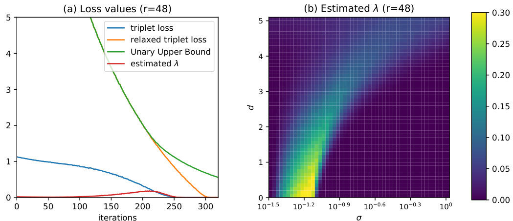
where $M_{t}=(\frac{n}{C})^{2}(C-1)$ and $\lambda>0$. The analytic form of $\lambda$ is intractable due to the unknown type of $g$ and the distribution of $\mathbf{h}_{i}$. We propose a toy example to show that $\lambda$ can be quite small. Denote $\mathbf{h}_{i}\in\mathbb{R}^{r},r=48$ in this example. Suppose there are $C=2$ clusters. Each cluster corresponds to a Gaussian distribution with covariance $\sigma\mathbf{I}_{r}$, and the distance between cluster centers (the means of Gaussian distributions) is $d$. The triplet ranking loss is defined as $g(a,b)=[a-b+1]_{+}$. During the training process, it is expected that $\sigma$ gradually decreases and $d$ gradually increases. Figure 2(a) shows the change of the original triplet loss, the Unary Upper Bound, and the triplet loss defined by the second term of Eq. (28) (denote relaxed triplet loss). An estimation of $\lambda\doteq(\mathcal{L}_{t}/M_{t}-\sum_{i=1}^{n}l_{c}(\mathbf{h}_{i},y_{i}))/\sum_{i=1}^{n}|\mathbf{h_{i}}-y_{i}|$ is also computed. It can be seen clearly that all losses are gradually decreasing and $\lambda$ is small during the whole process. Figure 2(b) illustrates the estimated $\lambda$ with varied $\sigma$ and $d$, which implies that $\lambda$ is relatively small under almost all conditions. Thus it is expected that a tighter Unary Upper Bound as Eq. (10) exists with a relatively small $\lambda$.

To conclude, the modified form of the Unary Upper Bound of the triplet loss can be written as Eq. (10), and we name it as Semantic Cluster Unary Loss(SCUL). By optimizing the SCUL in Eq. (10), not only a smaller $|\mathbf{h}_{i}-\mathbf{c}_{y_{i}}|$ but also a larger $|\mathbf{h}_{i}-\mathbf{c}_{y_{k}}|,y_{i}\neq y_{k}$ can be achieved, so that the original triplet loss is able to be minimized. Moreover, optimizing Eq. (10) is expected to be efficient as the complexity is just $O(n)$.

In the previous section, we have just considered hashing on data with single semantic label. In practical applications, lots of data have more than one semantic label, and the similarity is defined by whether two data instances share certain amount of labels. Hashing on data with multilabel should be considered.

Consider a case where semantic labels are evenly distributed. In particular, the probability of each $\mathbf{x}_{i},i=1,...,n$ has a certain label $l\in\{1,...,C\}$ is $p$. Denote that the similarity is defined by whether two data instances share at least one semantic label, and the triplet ranking loss is defined by

where $r_{ij}\geq 1$ denotes the number of labels $\mathbf{x}_{i}$ and $\mathbf{x}_{j}$ share. Note that we attach greater importance to similar data pairs with more shared semantic labels. Then we can arrive at an Unary Upper Bound of the above triplet ranking loss, which is concluded in the following proposition:

The proof of this proposition is shown in the supplemental material. Similar as Section III-C, we can arrive at a more general form such that

where $M_{mt}$ is a constant and the value of $u(x)$ is relatively small. Eq. (37) can be regraded as the multilabel version of SCUL and the complexity is also reduced to $O(n)$.

The overall network architecture is shown in Figure 3. Denote $\mathrm{fc7}$ as the last but one layer of a classification network (eg. AlexNet, VGGNet, etc.), there are two ways after $\mathrm{fc7}$. One way consists of two fully connected layers without non-linear activations. The first layer is the hashing layer with $r$ outputs, and the second layer has $C$ outputs. $\mathbf{C}=[\mathbf{c}_{1},...,\mathbf{c}_{C}]\in\mathbb{R}^{r\times C}$ is the parameters of the second layer, which can be regarded as $C$ cluster centers. The other way is a fully-connected layer(denote $\mathrm{fc8}$) with the softmax classification loss.

Denote $F(\mathbf{x})$ as the activations of the hashing layer, and $H(\mathbf{x})=\mathrm{sgn}(F(\mathbf{x}))$ as the hash function, where $\mathrm{sgn}$ is the element-wise sign function and $F(\mathbf{x})\in\mathbb{R}^{r}$. The objective is learning $F$ and $\mathbf{C}$ by optimizing the SCUL to obtain a good hash function.

After training the network, the binary codes of data $\mathbf{x}$ are easily obtained with $\mathbf{h}=\mathrm{sgn}(F(\mathbf{x}))$.

Denote $\mathbf{h}_{i}=\mathrm{sgn}(F(\mathbf{x}_{i})),i=1,2,...,n$, we should optimize the SCUL such that

We regard $|\cdot|$ as the euclidean distance in Eq. (16). As discussed before, the complexity of the proposed loss is just $O(n)$ and the loss has theoretical relationship with the triplet ranking loss. Similar as [13, 56], For faster convergence, we add another classification loss $\mathcal{L}_{1}=\sum_{i=1}^{n}l_{1}(\mathbf{x}_{i},y_{i})$ to train the deep neural network:

Inspired by deep methods for classification problems, for hashing on data with single label, $l_{c}(\mathbf{h}_{i},y_{i})$ has a similar form with softmax loss such that $l_{c}(\mathbf{h}_{i},y_{i})=-\log\frac{\exp(-|\mathbf{h}_{i}-\mathbf{c}_{y_{i}}|)}{\sum_{j=1}^{C}\exp(-|\mathbf{h}_{i}-\mathbf{c}_{j}|)}$.

For datasets with multilabels, $l_{c}(\mathbf{h}_{i},y_{i})+\lambda|\mathbf{h}_{i}-\mathbf{c}_{y_{i}}|$ can be replaced by $q(|Y_{i}|)l_{mc}(\mathbf{h}_{i},Y_{i})+\lambda\sum_{s\in Y_{i}}|\mathbf{h}_{i}-\mathbf{c}_{s}|$, where $l_{mc}(\mathbf{h}_{i},Y_{i})$ is defined in Eq. (14) and we simply use $q(x)=1/x$. $l_{1}(\mathbf{x}_{i},y_{i})$ is the multilabel softmax loss.

Note that $\mathcal{L}_{u}$ has a similar formulation with CenterLoss [54] to some extent, but the differences between two losses are obvious. First, CenterLoss just use softmax loss after the feature embedding layer, and the centers in the CenterLoss have no relationship with the last fully-connected layer. Second, our proposed $\mathcal{L}_{u}$ has the theoretical relationship with the triplet ranking loss. Furthermore, SCDH has a simple but novel extension of the multilabel case.

The main difficulty in optimizing Eq. (17) is the existence of the discrete constraints, making it intractable to train the network with back-propagation. Recent researches convey that removing the discrete constraints as well as adding the quantization loss is a good approach [64, 28, 4] in which the activation of the hashing layer $F(\mathbf{x})$ is not only continuous but also around $+1/-1$. However, optimizing these losses has to make the norm of $F(\mathbf{x})$ constrained. In fact, we just need to push the elements of the learned $F(\mathbf{x})$ away from zero so that less discrepancy is involved after generating the codes with the $\mathrm{sgn}$ function. For a well-learned $F(\mathbf{x})$ with relatively small or large norm, we may not necessarily optimize with the traditional quantization loss. [3]

In this paper, we introduce a new quantization loss such that $l_{q}(\mathbf{f})=1-\frac{\mathbf{1}^{\mathrm{T}}\mathrm{abs}(\mathbf{f})}{\|\mathbf{1}\|_{q}\|\mathbf{f}\|_{p}}$ and arrive at the following relaxed problem:

where $\mathrm{abs}(\cdot)$ is the element-wise absolute function, $\|\cdot\|_{p},\|\cdot\|_{q}$ form a pair of dual norms such that $1/p+1/q=1$, and therefore $\mathrm{abs}(\mathbf{x})^{\mathrm{T}}\mathrm{abs}(\mathbf{y})\leq\|\mathbf{x}\|_{p}\|\mathbf{y}\|_{q}$ for any $\mathbf{x},\mathbf{y}$ according to the Holder’s inequality. As shown in Figure 4, by optimizing the proposed quantization loss, each element of $F(\mathbf{x})$ is expected to be almost the same, thus less discrepancy between $F(\mathbf{x})$ and $\mathrm{sgn}(F(\mathbf{x}))$ will be involved. Moreover, unlike the quantization losses proposed in [64, 4], ours do not need to constrain the norm of $F(\mathbf{x})$ during optimization.

It is easier to optimize the quantization loss with greater $p$. We use $p=3,q=1.5$ in this algorithm.

It it clear that the proposed SCDH can be trained end-to-end with back-propagation, in which Eq. (18) can be optimized with gradient descent. The crucial term in Eq. (18) for gradient descent is the SCUL term, denoting $l_{u}(\mathbf{x}_{i})=l_{c}(F(\mathbf{x}_{i}),y_{i})+\lambda|F(\mathbf{x}_{i})-\mathbf{c}_{y_{i}}|$, and the gradient is computed as

where $p_{k}=\frac{\exp(-|\mathbf{h}_{i}-\mathbf{c}_{k}|)}{\sum_{j=1}^{C}\exp(-|\mathbf{h}_{i}-\mathbf{c}_{j}|)}$ can be regarded as the probability, and $\nabla|F(\mathbf{x}_{i})-\mathbf{c}_{j}|=(F(\mathbf{x}_{i})-\mathbf{c}_{j})/|F(\mathbf{x}_{i})-\mathbf{c}_{j}|$ is the gradient of the distance. By using Eq. (19), the network is able to be optimized end-to-end with back-propagation.

However, when training the dataset with a large number of classes like Imagenet, we find that the optimization of Eq. (18) may be hard to converge. We find that $p_{k},k=1,...,C$ will be relatively small in the beginning, especially on large number of classes, thus $\nabla_{\mathbf{c}_{y_{i}}}|F(\mathbf{x}_{i})-\mathbf{c}_{y_{i}}|,\nabla_{F(\mathbf{x}_{i})}|F(\mathbf{x}_{i})-\mathbf{c}_{y_{i}}|$ will take the crucial part in computing the gradients. In this case, $F(\mathbf{x}_{i}),\mathbf{c}_{y_{i}}$ may be encouraged to go to zero to make $|F(\mathbf{x}_{i})-\mathbf{c}_{y_{i}}|=0$, and we pay less attention to enlarging the inter-class distances, making the optimization hard to converge or even collapse.

To overcome the above issue, we propose a warm-up procedure before training directly with back-propagation. In the beginning epochs, we simply constrain the Semantic Cluster centers $\mathbf{C}$ to a certain norm $s$ to avoid the centers and $F(\mathbf{x}_{i})$ to go zero. After the warm-up procedure, $p_{y_{i}}$ goes larger, then the importance of $\nabla|F(\mathbf{x}_{i})-\mathbf{c}_{y_{i}}|$ is diminished and $F(\mathbf{x}_{i}),\mathbf{c}_{y_{i}}$ is hard to go zero. Moreover, a larger $F(\mathbf{x}_{i})$ makes it easier to enlarge the inter-class distances. For relatively small datasets, we do not need to use the warm-up procedure, but for faster convergence, the centers should be randomly initialized such that the norms of the centers should be large enough to prevent them going zero.

Mean Teacher [50] is the current state-of-the-art algorithm for semi-supervised learning. It assumes that the data predictions should be consistent under different perturbations, so that it can satisfy the smoothness assumption. In this case, Mean Teacher proposes a dual role, i.e., the teacher and the student. The student is learned as before; the teacher is the average of consecutive student models in which the weights are updated as an exponential moving average(EMA) of the student weights. In addition, the outputs of the teacher are regarded as targets for the training the student, so we can introduce the following consistency loss as regularization for training:

where $\mathcal{S},\mathcal{U}$ are the labeled and unlabeled datasets respectively, $\tilde{\mathbf{x}}^{(1)},\tilde{\mathbf{x}}^{(2)}$ are two random perturbations of the original data point $\mathbf{x}$, $f(\cdot),f_{T}(\cdot)$ are the outputs of student or teacher network respectively, and $d(\cdot,\cdot)$ is the distance between two features. In particular, the teacher can be regarded as the average ensemble of the student, thus $f_{T}(\cdot)$ can be regarded as the mean of the student’s outputs, making the training of the consistency loss more stable.

As the proposed SCUL is a classification-based unary loss, it can be easily incorporated with the Mean Teacher for semi-supervised hashing in MT-SCDH. MT-SCDH is also a teacher-student model which is shown in Figure 5. The student is learned in the same manner as SCDH with the labeled dataset. The teacher is updated in the same way as the Mean Teacher. For all training data, we apply the consistency loss among the outputs of the networks.

Denote $\mathcal{S}=\{(\mathbf{x}_{1},y_{1}),...,(\mathbf{x}_{n},y_{n})\}$ as the labeled data and $\mathcal{U}=\mathbf{x}_{n+1},...,\mathbf{x}_{m}$ as the unlabeled data. The learning problem of MT-SCDH is shown as follows:

where $d(\cdot,\cdot)=\|\mathrm{softmax}(\cdot)-\mathrm{softmax}(\cdot)\|^{2}$, $\mathcal{L}$ is the supervised term defined in Eq. (18), $l_{q}(\cdot)$ is the quantization loss proposed in Sec. IV-C, $w$ is the weight of the consistency loss, $\mathbf{a}_{i},\mathbf{a}_{i}^{T}$ are the outputs of $\mathrm{fc8}$ for $\mathbf{x}_{i}$ in the student and teacher network respectively, $\mathbf{d}_{i},\mathbf{d}_{i}^{T}$ denote the negative distances between $F(\mathbf{x}_{i})$ and the semantic clusters in the student and teacher network respectively. In other words, $\mathbf{d}_{i}=-[|F(\mathbf{x}_{i})-\mathbf{c}_{1}|,...,|F(\mathbf{x}_{i})-\mathbf{c}_{C}|]^{\mathrm{T}}$, and so as $\mathbf{d}_{i}^{T}$. Note that the input $\mathbf{x}_{i}$ is the random perturbations.

The basic configurations and training procedure are almost the same as SCDH. And we follow the suggested configurations (e.g. the value of $w$) in [50] for semi-supervised learning.

After training the network. we can extract the codes from either the teacher network or the student network.

In this section, we run large-scale retrieval experiments on three image benchmarks: CIFAR-10¹¹ 1 http://www.cs.toronto.edu/~kriz/cifar.html, Nuswide²² 2 http://lms.comp.nus.edu.sg/research/NUS-WIDE.htm and ImageNet³³ 3 http://image-net.org. CIFAR-10 consists of 60,000 $32\times 32$ color images from 10 object categories. ImageNet dataset is obtained from ILSVRC2012 dataset, which contains more than 1.2 million training images of 1,000 categories in total, together with 50,000 validation images. Nuswide dataset contains about 270K images collected from Flickr, and about 220K images are available from the Internet now. It associates with 81 ground truth concept labels, and each image contains multiple semantic labels. Following [35], we only use the images associated with the 21 most frequent concept tags, where the total number of images is about 190K, and the number of images associated with each tag is at least 5,000.

The experimental protocols are similar to [56]. In CIFAR-10 dataset, we randomly select 1,000 images (100 images per class) as the query set, and the rest 59,000 images as the retrieval database. In ImageNet dataset, the provided training set are used for retrieval database, and 50,000 validation images for the query set. In Nuswide dataset, we randomly select 2,100 images (100 images per class) as the query set. For CIFAR-10 and ImageNet, similar data pairs share the same semantic label. For Nuswide dataset, similar images share at least one semantic label.

Our method is implemented with PyTorch⁴⁴ 4 http://pytorch.org/ framework. We use pre-trained network parameters before $\mathrm{fc7}$ if necessary, and the parameters after $\mathrm{fc7}$ is initialized by ”Gaussian” initializer with zero mean and standard deviation 0.01, except the Semantic Clusters $\mathbf{C}$ which are initialized with standard deviation 0.5 to make the norms of clusters larger. The images are resized to the proper input sizes to train the network (e.g. $224\times 224$ for AlexNet and VGGNet). SGD is used for optimization, the momentum is 0.9 and the initial learning rate is set to 0.001 before $\mathrm{fc7}$ and 0.01 for the rest of layers.

For training the deep hashing network, we randomly select 5,000 images (500 per class) in CIFAR-10 and 10,500 images (500 per class) in Nuswide to train the network, and use all database images in the ImageNet dataset for training. For semi-supervised hashing methods, the remaining database data are regraded as unlabeled samples. The hyper-parameters $\lambda,\mu,\alpha$ is different according to datasets, which are selected with the validation set. We first of all randomly select part of training data as the validation set to determine the parameters. For CIFAR-10, we choose $\{\lambda=0.005,\mu=0.2,\alpha=0.05\}$ and the learning rate decreases by 80% after 100,140 epochs and stops at 160 epochs. For Nuswide, we select $\{\lambda=0.001,\mu=0.1,\alpha=1.0\}$ and the learning rate decreases by 80% after 40 epochs and stops at 60 epochs. For ImageNet we select $\{\lambda=0.001,\mu=0.1,\alpha=4.0\}$ and the learning rate decreases by 80% after 12, 17 epochs and stops at 20 epochs. Detailed parameter selection strategies are discussed in Sec. VI-E. Unless specified, we just use the warm-up procedure for training ImageNet in which the norms of Semantic Cluster centers $\mathbf{C}$ are constrained to $s=8$ in the first 5 epochs. The training is done on a server with two Intel(R) Xeon(R) E5-2683 v3@2.0GHz CPUs, 256GB RAM and a Geforce GTX TITAN Pascal with 12GB memory.

Similar to [34, 56], for each retrieval dataset, we report the compared results in terms of mean average precision(MAP), precision at Hamming distance within 2, and precision of top returned candidates. For Nuswide, we calculate the MAP value within the top 5000 returned neighbors, and we report the MAP of all retrieved samples on CIFAR-10. Groundtruths are defined by whether two candidates are similar. We run each experiment for 5 times and get the average result.

We compare our SCDH method with recent state-of-the-art deep hashing methods, including pairwise based methods such as DSH [31], DHN [64], DPSH [28], DQN [4], DISH [63], DSDH [27], triplet based methods like NINH [22], FTDE [65], BOH [6], DRLIH [61], and unary loss based methods like CNNBH [13], SSDH [59]. They follow similar experimental settings, but different methods may use different deep networks, thus we train on several types of network (AlexNet, VGGNet, ResNet, etc.) for fair comparison.

Retrieval results of different methods are shown in Table I,II,III and Figure 6. Note that the results with citations are copied from the corresponding papers, and some results are our own implementation with suggested parameters of the original paper. With the network structure fixed, our SCDH algorithm achieves better performance than methods with pairwise or triplet losses like NINH, DHN, DPSH, DSH and BOH, especially on CIFAR-10, showing the effectiveness of the proposed SCUL. As the discrete hashing methods like DISH and DSDH cannot be trained directly by back-propagation due to the special consideration of the discrete constraints, our SCDH method performs better than those methods. Moreover, our method performs better than the unary loss based methods like CNNBH and SSDH on most settings, showing that the proposed SCUL is friendly with the distance learning. It should be noticed that the classification performance of VGG-F net is slightly better than AlexNet, thus the hashing performance is expected not to decrease and may even get better if replacing AlexNet with VGG-F.

As the similarity information is defined by the semantic labels, it seems more simple to directly convert the predicted label to binary codes. As discussed in [45], we can encode the predicted label with one-hot binary codes, or convert the class probability to binary codes using LSH. We name these two methods as Cls-onehot and Cls-LSH respectively. Results on CIFAR-10 dataset are shown in Table I and Figure 6. The performances are lower than many hashing methods. Similar conclusion is arrived at [51], which shows that latent features extracted from fc6/fc7 contain more semantic information than the class probability features. Moreover, one-hot encodings lose more information than the class probabilities, thus Cls-onehot performs inferior than Cls-LSH.

Table IV summarizes the training time of some state-of-the-art methods. VGG-16 net is used for evaluation. As expected, the training speed of the proposed method is much faster than most deep hashing methods with pairwise losses or triplet losses. It takes less than 1 hour to generate good binary codes by the VGG-16 net, thus we can also train binary codes efficiently with deep neural nets.

We compare our MT-SCDH method with recent state-of-the-art semi-supervised deep hashing methods including SemiSDH [60], BGDH [57]. AlexNet is used for fair comparison. As suggested in [50], we use $w=50$ in the experiments. Retrieval results are shown in Table V. It is clear that the MT-SCDH algorithm performs much better than others by over 2 percents. Compared with the results of SCDH shown in Table I and II, the semi-supervised setting achieves better MAP value by about 0.3-2 percents, showing that the Mean Teacher based semi-supervised hashing approach is able to capture more semantic information with the unlabeled data.

Variants of SCDH In order to verify the effectiveness of our method, several variants of the proposed method are also considered. First, we regard $\mathcal{L}_{u}$ as just softmax loss such that $\lambda=0,l_{c}(\mathbf{h}_{i},y_{i})=-\log\frac{\exp\mathbf{c}_{y_{i}}^{\mathrm{T}}\mathbf{h}_{i}}{\sum_{l=1}^{C}\exp\mathbf{c}_{l}^{\mathrm{T}}\mathbf{h}_{i}}$. It is very similar with CNNBH [13] and we name it as SCDH-S. Second, we apply CenterLoss [54] for hashing, denote SCDH-C, in which $\mu=0$ and we replace $\mathcal{L}_{u}$ with the softmax loss and centerloss defined in [54]. Inspired by the SCUL in multilabel case, we extend the CenterLoss to the multilabel case for SCDH-C such that

Retrieval results are shown in Table VI. It is clear that SCDH and its variants perform better than most deep hashing algorithms. In particular, the proposed SCDH algorithm performs better than the variants, especially on the precision at Hamming distance within 2 value. Moreover, SCDH performs much better on Nuswide dataset, showing the effectiveness of the SCUL over the modified CenterLoss and the softmax loss on the multilabel version.

To address the above issue, Figure 7(a) shows the average intra-class distances of the normalized real-value representations $F(\mathbf{x})$ and hashcodes $\mathrm{sgn}(F(\mathbf{x}))$ of the training set. It is clear that the intra-class distances of the representations learned by SCDH is much smaller than those learned by the variants, thus SCDH is more likely to hash more similar data to the same hashcode, improving the precision at Hamming distance within 2 value. Figure 7(b-d) are t-SNE visualizations of the normalized $F(\mathbf{x})$ trained by SCDH and its variants. The clusters learned by SCDH is more compact than the variants, and there are less outliers in SCDH. Furthermore, some outliers in SCDH-S and SCDH-C goes to other clusters (like label 0 in SCDH-S and label 3 in SCDH-C). To conclude, the proposed SCUL have close relationship with the triplet ranking loss and get better results than CenterLoss and softmax loss, especially on the multilabel case.

The warm-up training procedure Another important issue is whether to use the warm-up procedure to optimize $\mathbf{C}$ for training datasets with large amount of labels. Table VII shows results on ImageNet dataset, which implies that the warm-up procedure performs better than the random initialization procedure. The performance of the warm-up procedure with different norms of clusters $s$ performs almost the same, including the average norm of the Semantic cluster centers after optimization, which implies that the results is not sensitive to $s$ in the warm-up procedure, thus we can set this parameter freely for training large datasets.

In this section, influence on different settings of the proposed SCDH algorithm is evaluated. We use AlexNet for pre-training, and the code length is 48.

Influence of $\alpha$ Figure 8(a)(b) shows the performance on different values of $\alpha$. It can be seen clearly that setting a certain $\alpha$ achieves better performance on either MAP or precision at Hamming distance within 2 value than setting $\alpha=0$. It means that adding the quantization loss improves the performance of hashing.

To get better hashcodes, a proper value of $\alpha$ should be set. Figure 9(a) shows the quantization loss at the end of training with different $\alpha$. Compared with 8(a)(b), $\alpha$ should be set to get the best performance in that the training quantization loss should be around $0.1\sim 0.2$.

Influence of $\lambda$ Figure 8(c)(d) shows the performance on different values of $\lambda$. It shows that a relatively small $\lambda$ leads to better performance on MAP. In fact, only optimizing $l_{c}(\mathbf{h}_{i},y_{i})$ is able to minimize the intra-class distances. Although $\lambda$ is not effective to get better MAP, greater value of precision at Hamming distance with 2 may be achieved when $\lambda$ goes larger, especially on the Nuswide dataset. It implies that the term $|\mathbf{h}_{i}-\mathbf{c}_{y_{i}}|$ is an auxiliary term to make intra-class smaller, thus more similar data is expected to map to the same hashcode.

Influence of $\mu$ Figure 8(e)(f) shows the performance on different values of $\mu$. It is shown that the algorithm is not too sensitive to $\mu$ over a wide range, but the performance is slightly better when $\mu\sim 0.1$, thus we recommend to set $\mu\sim 0.1$.

Figure 9(b) shows the MAP value with different training epochs on CIFAR-10 dataset. It can be seen clearly that a larger $\mu$ makes the training procedure faster, showing that setting proper $\mu$ is helpful for faster convergence.

References

- [1] M. Arjovsky, S. Chintala, and L. Bottou. Wasserstein generative adversarial networks. In International Conference on Machine Learning, pages 214–223, 2017.
- [2] F. Cakir, K. He, S. A. Bargal, and S. Sclaroff. Mihash: Online hashing with mutual information. In 2017 IEEE International Conference on Computer Vision (ICCV), pages 437–445. IEEE, 2017.
- [3] Y. Cao, M. Long, and J. Wang. Correlation hashing network for efficient cross-modal retrieval. CoRR, abs/1602.06697, 2016.
- [4] Y. Cao, M. Long, J. Wang, H. Zhu, and Q. Wen. Deep quantization network for efficient image retrieval. In AAAI, pages 3457–3463, 2016.
- [5] M. S. Charikar. Similarity estimation techniques from rounding algorithms. In Proceedings of the thiry-fourth annual ACM symposium on Theory of computing, pages 380–388. ACM, 2002.
- [6] Q. Dai, J. Li, J. Wang, and Y.-G. Jiang. Binary optimized hashing. In Proceedings of the 2016 ACM on Multimedia Conference, pages 1247–1256. ACM, 2016.
- [7] M. Datar, N. Immorlica, P. Indyk, and V. S. Mirrokni. Locality-sensitive hashing scheme based on p-stable distributions. In Proceedings of the twentieth annual symposium on Computational geometry, pages 253–262. ACM, 2004.
- [8] C. Elkan. Using the triangle inequality to accelerate k-means. In Proceedings of the 20th International Conference on Machine Learning (ICML-03), pages 147–153, 2003.
- [9] A. Gionis, P. Indyk, R. Motwani, et al. Similarity search in high dimensions via hashing. In VLDB, volume 99, pages 518–529, 1999.
- [10] J. Goldberger, G. E. Hinton, S. T. Roweis, and R. R. Salakhutdinov. Neighbourhood components analysis. In Advances in neural information processing systems, pages 513–520, 2005.
- [11] Y. Gong, S. Lazebnik, A. Gordo, and F. Perronnin. Iterative quantization: A procrustean approach to learning binary codes for large-scale image retrieval. Pattern Analysis and Machine Intelligence, IEEE Transactions on, 35(12):2916–2929, 2013.
- [12] Y. Gu, C. Ma, and J. Yang. Supervised recurrent hashing for large scale video retrieval. In Proceedings of the 2016 ACM on Multimedia Conference, pages 272–276. ACM, 2016.
- [13] J. Guo, S. Zhang, and J. Li. Hash learning with convolutional neural networks for semantic based image retrieval. In Pacific-Asia Conference on Knowledge Discovery and Data Mining, pages 227–238. Springer, 2016.
- [14] Y. Hao, T. Mu, J. Y. Goulermas, J. Jiang, R. Hong, and M. Wang. Unsupervised t-distributed video hashing and its deep hashing extension. IEEE Transactions on Image Processing, 26(11):5531–5544, 2017.
- [15] K. He, X. Zhang, S. Ren, and J. Sun. Deep residual learning for image recognition. In Proceedings of the IEEE Conference on Computer Vision and Pattern Recognition, pages 770–778, 2016.
- [16] J. Ji, J. Li, Q. Tian, S. Yan, and B. Zhang. Angular-similarity-preserving binary signatures for linear subspaces. IEEE Transactions on Image Processing, 24(11):4372–4380, 2015.
- [17] J. Ji, J. Li, S. Yan, Q. Tian, and B. Zhang. Min-max hash for jaccard similarity. In 2013 IEEE 13th International Conference on Data Mining, pages 301–309. IEEE, 2013.
- [18] W. Kong and W.-J. Li. Isotropic hashing. In Advances in Neural Information Processing Systems, pages 1646–1654, 2012.
- [19] A. Krause, P. Perona, and R. G. Gomes. Discriminative clustering by regularized information maximization. In Advances in neural information processing systems, pages 775–783, 2010.
- [20] A. Krizhevsky, I. Sutskever, and G. E. Hinton. Imagenet classification with deep convolutional neural networks. In Advances in neural information processing systems, pages 1097–1105, 2012.
- [21] B. Kulis and T. Darrell. Learning to hash with binary reconstructive embeddings. In Advances in neural information processing systems, pages 1042–1050, 2009.
- [22] H. Lai, Y. Pan, Y. Liu, and S. Yan. Simultaneous feature learning and hash coding with deep neural networks. In The IEEE Conference on Computer Vision and Pattern Recognition (CVPR), June 2015.
- [23] H. Lai, P. Yan, X. Shu, Y. Wei, and S. Yan. Instance-aware hashing for multi-label image retrieval. IEEE Transactions on Image Processing, 25(6):2469–2479, 2016.
- [24] S. Laine and T. Aila. Temporal ensembling for semi-supervised learning. arXiv preprint arXiv:1610.02242, 2016.
- [25] P. Li and C. König. b-bit minwise hashing. In Proceedings of the 19th international conference on World wide web, pages 671–680. ACM, 2010.
- [26] P. Li, A. Shrivastava, J. L. Moore, and A. C. König. Hashing algorithms for large-scale learning. In Advances in neural information processing systems, pages 2672–2680, 2011.
- [27] Q. Li, Z. Sun, R. He, and T. Tan. Deep supervised discrete hashing. arXiv preprint arXiv:1705.10999, 2017.
- [28] W.-J. Li, S. Wang, and W.-C. Kang. Feature learning based deep supervised hashing with pairwise labels. In IJCAI, pages 1711–1717, 2016.
- [29] G. Lin, C. Shen, Q. Shi, A. van den Hengel, and D. Suter. Fast supervised hashing with decision trees for high-dimensional data. In Computer Vision and Pattern Recognition (CVPR), 2014 IEEE Conference on, pages 1971–1978. IEEE, 2014.
- [30] G. Lin, C. Shen, and A. van den Hengel. Supervised hashing using graph cuts and boosted decision trees. IEEE Transactions on Pattern Analysis and Machine Intelligence, 2015.
- [31] H. Liu, R. Wang, S. Shan, and X. Chen. Deep supervised hashing for fast image retrieval. In Proceedings of the IEEE Conference on Computer Vision and Pattern Recognition, pages 2064–2072, 2016.
- [32] L. Liu, Z. Lin, L. Shao, F. Shen, G. Ding, and J. Han. Sequential discrete hashing for scalable cross-modality similarity retrieval. IEEE Transactions on Image Processing, 26(1):107–118, 2017.
- [33] W. Liu, C. Mu, S. Kumar, and S.-F. Chang. Discrete graph hashing. In Advances in Neural Information Processing Systems, pages 3419–3427, 2014.
- [34] W. Liu, J. Wang, R. Ji, Y.-G. Jiang, and S.-F. Chang. Supervised hashing with kernels. In Computer Vision and Pattern Recognition (CVPR), 2012 IEEE Conference on, pages 2074–2081. IEEE, 2012.
- [35] W. Liu, J. Wang, S. Kumar, and S.-F. Chang. Hashing with graphs. In Proceedings of the 28th international conference on machine learning (ICML-11), pages 1–8, 2011.
- [36] W. Liu, Y. Wen, Z. Yu, M. Li, B. Raj, and L. Song. Sphereface: Deep hypersphere embedding for face recognition. arXiv preprint arXiv:1704.08063, 2017.
- [37] X. Liu, J. He, and S.-F. Chang. Hash bit selection for nearest neighbor search. IEEE Transactions on Image Processing, 26(11):5367–5380, 2017.
- [38] J. Lu, V. Erin Liong, and J. Zhou. Deep hashing for scalable image search. IEEE Transactions on Image Processing, 26(5):2352–2367, 2017.
- [39] Y. Luo, J. Zhu, M. Li, Y. Ren, and B. Zhang. Smooth neighbors on teacher graphs for semi-supervised learning. arXiv preprint arXiv:1711.00258, 2017.
- [40] Y. Movshovitz-Attias, A. Toshev, T. K. Leung, S. Ioffe, and S. Singh. No fuss distance metric learning using proxies. In The IEEE International Conference on Computer Vision (ICCV), Oct 2017.
- [41] M. Norouzi and D. M. Blei. Minimal loss hashing for compact binary codes. In Proceedings of the 28th international conference on machine learning (ICML-11), pages 353–360, 2011.
- [42] M. Norouzi, D. J. Fleet, and R. R. Salakhutdinov. Hamming distance metric learning. In Advances in neural information processing systems, pages 1061–1069, 2012.
- [43] O. M. Parkhi, A. Vedaldi, A. Zisserman, et al. Deep face recognition. In BMVC, volume 1, page 6, 2015.
- [44] S. Ren, K. He, R. Girshick, and J. Sun. Faster r-cnn: Towards real-time object detection with region proposal networks. In Advances in Neural Information Processing Systems, pages 91–99, 2015.
- [45] A. Sablayrolles, M. Douze, N. Usunier, and H. Jégou. How should we evaluate supervised hashing? In Acoustics, Speech and Signal Processing (ICASSP), 2017 IEEE International Conference on, pages 1732–1736. IEEE, 2017.
- [46] F. Schroff, D. Kalenichenko, and J. Philbin. Facenet: A unified embedding for face recognition and clustering. In Proceedings of the IEEE Conference on Computer Vision and Pattern Recognition, pages 815–823, 2015.
- [47] F. Shen, C. Shen, W. Liu, and H. Tao Shen. Supervised discrete hashing. In The IEEE Conference on Computer Vision and Pattern Recognition (CVPR), June 2015.
- [48] K. Simonyan and A. Zisserman. Very deep convolutional networks for large-scale image recognition. arXiv preprint arXiv:1409.1556, 2014.
- [49] Y. Sun, Y. Chen, X. Wang, and X. Tang. Deep learning face representation by joint identification-verification. In Advances in neural information processing systems, pages 1988–1996, 2014.
- [50] A. Tarvainen and H. Valpola. Mean teachers are better role models: Weight-averaged consistency targets improve semi-supervised deep learning results. In Advances in neural information processing systems, pages 1195–1204, 2017.
- [51] J. Wan, D. Wang, S. C. H. Hoi, P. Wu, J. Zhu, Y. Zhang, and J. Li. Deep learning for content-based image retrieval: A comprehensive study. In Proceedings of the ACM International Conference on Multimedia, pages 157–166. ACM, 2014.
- [52] J. Wang, S. Kumar, and S.-F. Chang. Semi-supervised hashing for large-scale search. Pattern Analysis and Machine Intelligence, IEEE Transactions on, 34(12):2393–2406, 2012.
- [53] Y. Weiss, A. Torralba, and R. Fergus. Spectral hashing. In Advances in neural information processing systems, pages 1753–1760, 2009.
- [54] Y. Wen, K. Zhang, Z. Li, and Y. Qiao. A discriminative feature learning approach for deep face recognition. In European Conference on Computer Vision, pages 499–515. Springer, 2016.
- [55] J. Weston, F. Ratle, H. Mobahi, and R. Collobert. Deep learning via semi-supervised embedding. In Neural Networks: Tricks of the Trade, pages 639–655. Springer, 2012.
- [56] R. Xia, Y. Pan, H. Lai, C. Liu, and S. Yan. Supervised hashing for image retrieval via image representation learning. In Proceedings of the AAAI Conference on Artificial Intellignece, pages 2156–2162, 2014.
- [57] X. Yan, L. Zhang, and W.-J. Li. Semi-supervised deep hashing with a bipartite graph. In Proceedings of the 26th International Joint Conference on Artificial Intelligence, pages 3238–3244. AAAI Press, 2017.
- [58] X. Yan, L. Zhang, and W.-J. Li. Semi-supervised deep hashing with a bipartite graph. In Proceedings of the 26th International Joint Conference on Artificial Intelligence, pages 3238–3244. AAAI Press, 2017.
- [59] H.-F. Yang, K. Lin, and C.-S. Chen. Supervised learning of semantics-preserving hash via deep convolutional neural networks. IEEE transactions on pattern analysis and machine intelligence, 40(2):437–451, 2018.
- [60] J. Zhang and Y. Peng. Ssdh: semi-supervised deep hashing for large scale image retrieval. IEEE Transactions on Circuits and Systems for Video Technology, 2017.
- [61] J. Zhang, Y. Peng, and Z. Ye. Deep reinforcement learning for image hashing. arXiv preprint arXiv:1802.02904, 2018.
- [62] R. Zhang, L. Lin, R. Zhang, W. Zuo, and L. Zhang. Bit-scalable deep hashing with regularized similarity learning for image retrieval and person re-identification. IEEE Transactions on Image Processing, 24(12):4766–4779, 2015.
- [63] S. Zhang, J. Li, M. Jiang, and B. Zhang. Scalable discrete supervised multimedia hash learning with clustering. IEEE Transactions on Circuits and Systems for Video Technology, 2017.
- [64] H. Zhu, M. Long, J. Wang, and Y. Cao. Deep hashing network for efficient similarity retrieval. In Thirtieth AAAI Conference on Artificial Intelligence, 2016.
- [65] B. Zhuang, G. Lin, C. Shen, and I. Reid. Fast training of triplet-based deep binary embedding networks. In Proceedings of the IEEE Conference on Computer Vision and Pattern Recognition, pages 5955–5964, 2016.
![[Uncaptioned image]](1805.08705v2/bio_ShifengZhang.png) |
Shifeng Zhang received the B.E. degree from the Department of Computer Science and Technology, Tsinghua University, in 2015. Now he is a Ph.D. student in the State Key Laboratory of Intelligent Technology and Systems, Beijing National Research Center for Information Science and Technology, Department of Computer Science and Technology, Tsinghua University. His supervisor is Prof. Bo Zhang. His current research interests include hashing method and deep metric learning. |