Fast Symbolic 3D Registration Solution

Jin Wu Ming Liu Zebo Zhou and Rui Li ^†^†thanks: Manuscript received May 29, 2018; revised January 3, 2019; accepted September 17, 2019. Date of publication September 17, 2019; date of current version September 17, 2019. This paper was recommended for publication by Associate Editor D. Liu and Editor Y. Sun upon evaluation of the reviewers’ comments. This research was supported by Shenzhen Science, Technology and Innovation Comission (SZSTI) JCYJ20160401100022706, awarded to Prof. Ming Liu., in part by National Natural Science Foundation of China under the grant of No. 41604025, in part by General Research Fund of Research Grants Council Hong Kong,11210017, and also in part by Early Career Scheme Project of Research Grants Council Hong Kong, 21202816. (Corresponding author: Ming Liu).^†^†thanks: J. Wu and M. Liu are with Department of Electrical & Computer Engineering, Hong Kong University of Science and Technology, Hong Kong, China. e-mail: jin_wu_uestc@hotmail.com; eelium@ust.hk^†^†thanks: Z. Zhou and R. Li are with University of Electronic Science and Technology of China, Chengdu, China. e-mail: klinsmann.zhou@gmail.com; hitlirui@gmail.com.^†^†thanks: Color versions of one or more of the figures in this paper are available online at http://ieeexplore.ieee.org.^†^†thanks: Digital Object Identifier 10.1109/TASE.2019.

Abstract

3D registration has always been performed invoking singular value decomposition (SVD) or eigenvalue decomposition (EIG) in real engineering practices. However, these numerical algorithms suffer from uncertainty of convergence in many cases. A novel fast symbolic solution is proposed in this paper by following our recent publication in this journal. The equivalence analysis shows that our previous solver can be converted to deal with the 3D registration problem. Rather, the computation procedure is studied for further simplification of computing without complex-number support. Experimental results show that the proposed solver does not loose accuracy and robustness but improves the execution speed to a large extent by almost %50 to %80, on both personal computer and embedded processor.

Note to Practitioners—3D registration usually has large computational burden in engineering tasks. The proposed symbolic solution can directly solve the eigenvalue and its associated eigenvector. A lot of computation resources can then be saved for better overall system performance. The deterministic behavior of the proposed solver also ensures long-endurance stability and can help engineer better design thread timing logic.

Index Terms:

3D Registration, Symbolic Computation, Numerical Algorithms, Fast Computation Speed, Robotics

I Introduction

Motion estimation from point correspondences is an important technique in robotics [1, 2, 3]. The point measurements can usually be acquired from laser scanner and camera for accurate relative attitude/position determination [4, 5]. The methodology behind is called the 3D registration which figures out the rigid transformation consisting of rotation and translation [6]. Yet, this technology is employed for 3D reconstruction of objects by means of multi-directional point-cloud snapshots, which extensively boosts the automation assembly [7, 8, 9]. Thanks to 3D registration, the image stitching can be performed accurately for better sequence processing [10]. And moreover, the navigation performance of intelligent vehicles can be improved by existing registration techniques [11, 12].
The basic 3D registration problem can usually be expressed as a least-square fitting one which takes the following form [13]

\mathop{\arg\min}\limits_{\bm{C}\in SO(3),\bm{T}\in\mathbb{R}^{3}}{\mathcal{L}}=\sum\limits_{i=1}^{n}{{a_{i}}{{\left\|{{{\bm{b}}_{i}}-{\bm{C}}{{\bm{r}}_{i}}-{\bm{T}}}\right\|}^{2}}}

(1)

where ${{{\bm{b}}_{i}}}\in\{{\cal{B}}\}$ and ${{{\bm{r}}_{i}}}\in\{{\cal{R}}\}$ are point measurement pair in the body and reference frames; $a_{i}$ is the positive weight associated with the $i$ -th point pair. The target is to estimate the direction cosine matrix ${\bm{C}}$ in the special orthogonal group $SO(3)$ such that ${\bm{C}}{{\bm{C}}^{T}}={\bm{I}},\det({\bm{C}})=+1$ , with ${\bm{T}}$ in the real 3D vector space $\mathbb{R}^{3}$ , to minimize the sum $\mathcal{L}$ . As there are both noise items inside ${{{\bm{b}}_{i}}}$ and ${{{\bm{r}}_{i}}}$ , the problem is actually a total least square (TLS) [14, 15]. In real engineering applications, $\{\cal{B}\}$ and $\{\cal{R}\}$ do not always agree in the dimension. So the problem (1) is usually dealt with using the iterative closest points (ICP) for robust matching [16]. Apart from ICP i.e. only find-based approach, the local geometric features inside the point clouds and images can also help for more robust matching [17]. Local geometric features are more advanced understanding and aspects inside data sequences and can reflect those regular and visualizable geometric characteristics [18, 19], which intrinsically enhance the performance of 3D registration in urban areas e.g. in applications of the lidar odometry and mapping in real-time (LOAM, [20, 21]). When there are rare local geometric features in the data, ICP is still generally feasible for processing global registration. Some algorithms have been proposed in the last 30 years to solve the $\bm{C}$ and $\bm{T}$ from (1) efficiently. The first famous solver was proposed by K. S. Arun et al. who introduces SVD for rotation estimation [22]. However, when the problem contains large noise density, only SVD can not give robust estimation. Umeyama improves Arun’s method by changing the signs of the singular values [23]. In fact, the only difficulty of the optimization (1) is that $\bm{C}$ is nonlinear. However, after parameterizing $\bm{C}$ with dual quaternion, the problem can also be solved [24]. A simpler approach is established by unit quaternions which converts the problem (1) into an EIG one [25]. In fair comparisons, the dual quaternion is the slowest while EIG is slightly slower than SVD [26]. But for both EIG and SVD, the numerical implementation requires many computation loads and space consumption of required libraries. This generates a difficulty for their usage on some critical platforms e.g. field programmable gate arrays (FPGA) and some low-configuration micro controller units (MCU) [27]. The current situation also sets an obstacle for mass production of specified low-power integrated circuit (IC).
Recently, we propose an algorithm for vector-observation attitude determination called the fast linear attitude estimator (FLAE) [28]. FLAE owns the much superior computation speed compared with previous representatives. Motivated by SVD, EIG and FLAE, in this paper, a novel symbolic method is proposed. Through tests, the algorithm is verified to have only %50 to %80 execution time of recent fast SVD and EIG by C++ implementation on both personal computer and the MCU. In section II we present how to relate (1) with FLAE together. A simplified algorithm of eigenvalue is derived as well in this section. Experimental validations are presented in section III while section IV consists of concluding remarks.

II Main Results

The FLAE actually solves a more specific variant of (1) where $\bm{T}=0$ and $\left\|{{{\bm{b}}_{i}}}\right\|=\left\|{{{\bm{r}}_{i}}}\right\|=1$ [28] which can be further extended to some optimized results [29]. This is a preliminary for attitude determination from normalized vector observations in spacecraft motion measurement. In FLAE, the DCM is parameterized by the unit quaternion. The optimal quaternion is associated with eigenvalue of $\bm{W}$ that is closest to 1 where $\bm{W}$ is given by

\begin{array}[]{l}{{\bm{W}}_{1,1}}={H_{x1}}+{H_{y2}}+{H_{z3}}\\ {{\bm{W}}_{1,2}}=-{H_{y3}}+{H_{z2}}\\ {{\bm{W}}_{1,3}}=-{H_{z1}}+{H_{x3}}\\ {{\bm{W}}_{1,4}}=-{H_{x2}}+{H_{y1}}\\ {{\bm{W}}_{2,1}}=-{H_{y3}}+{H_{z2}}\\ {{\bm{W}}_{2,2}}={H_{x1}}-{H_{y2}}-{H_{z3}}\\ {{\bm{W}}_{2,3}}={H_{x2}}+{H_{y1}}\\ {{\bm{W}}_{2,4}}={H_{x3}}+{H_{z1}}\\ {{\bm{W}}_{3,1}}=-{H_{z1}}+{H_{x3}}\\ {{\bm{W}}_{3,2}}={H_{x2}}+{H_{y1}}\\ {{\bm{W}}_{3,3}}={H_{y2}}-{H_{x1}}-{H_{z3}}\\ {{\bm{W}}_{3,4}}={H_{y3}}+{H_{z2}}\\ {{\bm{W}}_{4,1}}=-{H_{x2}}+{H_{y1}}\\ {{\bm{W}}_{4,2}}={H_{x3}}+{H_{z1}}\\ {{\bm{W}}_{4,3}}={H_{y3}}+{H_{z2}}\\ {{\bm{W}}_{4,4}}={H_{z3}}-{H_{y2}}-{H_{x1}}\end{array}

(2)

in which ${\bm{W}}_{i,j}$ denotes the matrix entry of $\bm{W}$ in the $i$ -th row and $j$ -th column. The parameters inside are provided as follows

{\bm{H}}=\left({\begin{array}[]{*{20}{c}}{{H_{x1}}}&{{H_{y1}}}&{{H_{z1}}}\\ {{H_{x2}}}&{{H_{y2}}}&{{H_{z2}}}\\ {{H_{x3}}}&{{H_{y3}}}&{{H_{z3}}}\end{array}}\right)=\sum\limits_{i=1}^{n}{{a_{i}}{{\bm{b}}_{i}}{\bm{r}}_{i}^{T}}

(3)

The characteristic polynomial of $\bm{W}$ takes the form of

{\lambda^{4}}+{\tau_{1}}{\lambda^{2}}+{\tau_{2}}\lambda+{\tau_{3}}=0

(4)

where

\begin{array}[]{*{20}{l}}{{\tau_{1}}=}{-2\left(\begin{array}[]{l}H_{x1}^{2}+H_{x2}^{2}+H_{x3}^{2}+H_{y1}^{2}\\ +H_{y2}^{2}+H_{y3}^{2}+H_{z1}^{2}+H_{z2}^{2}+H_{z3}^{2}\end{array}\right)}\\ {{\tau_{2}}=}{8({H_{x3}}{H_{y2}}{H_{z1}}-{H_{x2}}{H_{y3}}{H_{z1}}-{H_{x3}}{H_{y1}}{H_{z2}}}\\ \ \ \ \ \ \ \ \ \ \ \ \ \ \ \ \ {+{H_{x1}}{H_{y3}}{H_{z2}}+{H_{x2}}{H_{y1}}{H_{z3}}-{H_{x1}}{H_{y2}}{H_{z3}})}\\ {{\tau_{3}}=\det({\bm{W}})}\end{array}

(5)

For the problem (1), the quaternion solution is produced by the optimal eigenvector of the following matrix [1, 16]

{\bm{G}}=\left[{\begin{array}[]{*{20}{c}}{tr({\bm{D}})}&{{{\bm{z}}^{T}}}\\ {\bm{z}}&{{\bm{D}}+{{\bm{D}}^{T}}-tr({\bm{D}}){\bm{I}}}\end{array}}\right]

(6)

in which

\begin{gathered}{\bm{D}}=\sum\limits_{i=1}^{n}{{a_{i}}({{\bm{b}}_{i}}-{\bm{\bar{b}}}){{({\bm{r}}_{i}-{\bm{\bar{r}}})}^{T}}}\hfill\\ {\bm{z}}=\sum\limits_{i=1}^{n}{{a_{i}}({{\bm{b}}_{i}}-{\bm{\bar{b}}})\times({\bm{r}}_{i}-{\bm{\bar{r}}})}\hfill\\ {\bm{\bar{b}}}=\sum\limits_{i=1}^{n}a_{i}{{{\bm{b}}_{i}}},{\bm{\bar{r}}}=\sum\limits_{i=1}^{n}a_{i}{{{\bm{r}}_{i}}}\hfill\\ \end{gathered}

(7)

It is obvious that $\bm{D}$ has the same structure with $\bm{H}$ . Then if $\bm{D}=H$ , we would like to prove that $\bm{G}=W$ . It can be directly obtained that

\begin{gathered}{\bm{D}}+{{\bm{D}}^{T}}-tr({\bm{D}}){\bm{I}}=\hfill\\ \small\left({\begin{array}[]{*{20}{c}}{{H_{x1}}-{H_{y2}}-{H_{z3}}}&{{H_{x2}}+{H_{y1}}}&{{H_{x3}}+{H_{z1}}}\\ {{H_{x2}}+{H_{y1}}}&{{H_{y2}}-{H_{x1}}-{H_{z3}}}&{{H_{y3}}+{H_{z2}}}\\ {{H_{x3}}+{H_{z1}}}&{{H_{y3}}+{H_{z2}}}&{{H_{z3}}-{H_{y2}}-{H_{x1}}}\end{array}}\right)\hfill\\ tr({\bm{D}})={H_{x1}}+{H_{y2}}+{H_{z3}}\hfill\\ \end{gathered}

(8)

For $\bm{z}$ , it has another form according to the skew-symmetric matrix of cross-product, such that

\begin{gathered}{\bm{z}}={\left({{{\bm{D}}_{2,3}}-{{\bm{D}}_{3,2}},{{\bm{D}}_{3,1}}-{{\bm{D}}_{1,3}},{{\bm{D}}_{1,2}}-{{\bm{D}}_{2,1}}}\right)^{T}}\hfill\\ \begin{array}[]{*{20}{c}}&\end{array}={\left({-{H_{y3}}+{H_{z2}},-{H_{z1}}+{H_{x3}},-{H_{x2}}+{H_{y1}}}\right)^{T}}\hfill\\ \end{gathered}

(9)

Inserting these results into (6), one can observe that $\bm{W}=G$ . So the characteristic polynomial of $\bm{W}$ can also be used for eigenvalue solving of $\bm{G}$ .
The FLAE gives the following symbolic roots of (4):

\begin{array}[]{l}{\lambda_{1}}=\frac{1}{{2\sqrt{6}}}\left({{T_{2}}-\sqrt{-T_{2}^{2}-12{\tau_{1}}-\frac{{12\sqrt{6}{\tau_{2}}}}{{{T_{2}}}}}}\right)\\ {\lambda_{2}}=\frac{1}{{2\sqrt{6}}}\left({{T_{2}}+\sqrt{-T_{2}^{2}-12{\tau_{1}}-\frac{{12\sqrt{6}{\tau_{2}}}}{{{T_{2}}}}}}\right)\\ {\lambda_{3}}=-\frac{1}{{2\sqrt{6}}}\left({{T_{2}}+\sqrt{-T_{2}^{2}-12{\tau_{1}}+\frac{{12\sqrt{6}{\tau_{2}}}}{{{T_{2}}}}}}\right)\\ {\lambda_{4}}=-\frac{1}{{2\sqrt{6}}}\left({{T_{2}}-\sqrt{-T_{2}^{2}-12{\tau_{1}}+\frac{{12\sqrt{6}{\tau_{2}}}}{{{T_{2}}}}}}\right)\end{array}

(10)

in which

\begin{array}[]{l}{T_{0}}=2\tau_{1}^{3}+27\tau_{2}^{2}-72\tau_{1}\tau_{3}\\ {T_{1}}={\left({{T_{0}}+\sqrt{-4{{\left({\tau_{1}^{2}+12\tau_{3}}\right)}^{3}}+T_{0}^{2}}}\right)^{\frac{1}{3}}}\\ {T_{2}}=\sqrt{-4\tau_{1}+\frac{{{2^{\frac{4}{3}}}\left({\tau_{1}^{2}+12\tau_{3}}\right)}}{{{T_{1}}}}+{2^{\frac{2}{3}}}{T_{1}}}\end{array}

(11)

Let us first determine the signs of $\tau_{1},\tau_{2},\tau_{3}$ . $\bm{W}$ is real symmetric and the eigenvalues are two positive and two negative. This gives $\tau_{3}=\det({\bm{W}})=\lambda_{1}\lambda_{2}\lambda_{3}\lambda_{4}>0$ . $\tau_{1}$ is obvious negative and $\tau_{2}$ is indefinite. In this way, $T_{0}$ is definitely real number. Let us write $T_{1},T_{2}$ into

\begin{gathered}{T_{1}}={\alpha_{{T_{1}}}}+{\beta_{{T_{1}}}}{\bm{i}}\hfill\\ {T_{2}}={\alpha_{{T_{2}}}}+{\beta_{{T_{2}}}}{\bm{i}}\hfill\\ \end{gathered}

(12)

where $\bm{i}$ denotes the unit imaginary number while ${\alpha_{{T_{1}}}},{\beta_{{T_{1}}}},{\alpha_{{T_{2}}}},{\beta_{{T_{2}}}}\in\mathbb{R}$ . Obviously, $T_{1}$ meets

\begin{gathered}T_{1}^{3}=\alpha_{{T_{1}}}^{3}-3{\alpha_{{T_{1}}}}\beta_{{T_{1}}}^{2}+\left({3\alpha_{{T_{1}}}^{2}{\beta_{{T_{1}}}}-\beta_{{T_{1}}}^{3}}\right){\bm{i}}\hfill\\ ={T_{0}}+\sqrt{-4{{\left({\tau_{1}^{2}+12{\tau_{3}}}\right)}^{3}}+T_{0}^{2}}\hfill\\ \end{gathered}

(13)

Likewise, we have

\begin{gathered}T_{2}^{2}=\alpha_{{T_{2}}}^{2}-\beta_{{T_{2}}}^{2}+2{\alpha_{{T_{2}}}}{\beta_{{T_{2}}}}{\bm{i}}\hfill\\ =-4{\tau_{1}}+\frac{{{2^{\frac{4}{3}}}\left({\tau_{1}^{2}+12{\tau_{3}}}\right)}}{{{T_{1}}}}+{2^{\frac{2}{3}}}{T_{1}}\hfill\\ =-4{\tau_{1}}+\frac{{{2^{\frac{4}{3}}}\left({\tau_{1}^{2}+12{\tau_{3}}}\right)}}{{{\alpha_{{T_{1}}}}+{\beta_{{T_{1}}}}{\bm{i}}}}+{2^{\frac{2}{3}}}\left({{\alpha_{{T_{1}}}}+{\beta_{{T_{1}}}}{\bm{i}}}\right)\hfill\\ =-4{\tau_{1}}+\left[{\sqrt[3]{4}+\frac{2{\sqrt[3]{2}\left({\tau_{1}^{2}+12{\tau_{3}}}\right)}}{{\alpha_{{T_{1}}}^{2}+\beta_{{T_{1}}}^{2}}}}\right]{\alpha_{{T_{1}}}}\hfill\\ \begin{array}[]{*{20}{c}}&\end{array}+\left[{\sqrt[3]{4}-\frac{2{\sqrt[3]{2}\left({\tau_{1}^{2}+12{\tau_{3}}}\right)}}{{\alpha_{{T_{1}}}^{2}+\beta_{{T_{1}}}^{2}}}}\right]{\beta_{{T_{1}}}}{\bm{i}}\hfill\\ \end{gathered}

(14)

These equations lead to the system of

\left\{{\begin{array}[]{*{20}{c}}{\alpha_{{T_{1}}}^{3}-3{\alpha_{{T_{1}}}}\beta_{{T_{1}}}^{2}={T_{0}}}\\ {{{\left({3\alpha_{{T_{1}}}^{2}{\beta_{{T_{1}}}}-\beta_{{T_{1}}}^{3}}\right)}^{2}}=4{{\left({\tau_{1}^{2}+12{\tau_{3}}}\right)}^{3}}-T_{0}^{2}}\\ {\alpha_{{T_{2}}}^{2}-\beta_{{T_{2}}}^{2}=-4{\tau_{1}}+\left[{\sqrt[3]{4}+\frac{{2\sqrt[3]{2}\left({\tau_{1}^{2}+12{\tau_{3}}}\right)}}{{\alpha_{{T_{1}}}^{2}+\beta_{{T_{1}}}^{2}}}}\right]{\alpha_{{T_{1}}}}}\\ {2{\alpha_{{T_{2}}}}{\beta_{{T_{2}}}}=\left[{\sqrt[3]{4}-\frac{{2\sqrt[3]{2}\left({\tau_{1}^{2}+12{\tau_{3}}}\right)}}{{\alpha_{{T_{1}}}^{2}+\beta_{{T_{1}}}^{2}}}}\right]{\beta_{{T_{1}}}}}\end{array}}\right.

(15)

From the first two sub-equations, one can easily arrive at

\begin{gathered}{\left({\alpha_{{T_{1}}}^{3}-3{\alpha_{{T_{1}}}}\beta_{{T_{1}}}^{2}}\right)^{2}}+{\left({3\alpha_{{T_{1}}}^{2}{\beta_{{T_{1}}}}-\beta_{{T_{1}}}^{3}}\right)^{2}}=4{\left({\tau_{1}^{2}+12{\tau_{3}}}\right)^{3}}\hfill\\ \Rightarrow\alpha_{{T_{1}}}^{6}+3\alpha_{{T_{1}}}^{4}\beta_{{T_{1}}}^{2}+3\alpha_{{T_{1}}}^{2}\beta_{{T_{1}}}^{4}+\beta_{{T_{1}}}^{6}=4{\left({\tau_{1}^{2}+12{\tau_{3}}}\right)^{3}}\hfill\\ \Rightarrow\alpha_{{T_{1}}}^{2}+\beta_{{T_{1}}}^{2}=\sqrt[3]{4}\left({\tau_{1}^{2}+12{\tau_{3}}}\right)\hfill\\ \end{gathered}

(16)

Inserting (16) into (15) we have

\left\{{\begin{array}[]{*{20}{c}}{\alpha_{{T_{2}}}^{2}-\beta_{{T_{2}}}^{2}=-4{\tau_{1}}+2\sqrt[3]{4}{\alpha_{{T_{1}}}}}\\ {2{\alpha_{{T_{2}}}}{\beta_{{T_{2}}}}=0}\end{array}}\right.

(17)

This indicates that ${\alpha_{{T_{2}}}}=0$ or ${\beta_{{T_{2}}}}=0$ . If ${\alpha_{{T_{2}}}}=0$ then $T_{2}$ is a pure imaginary number leading to the eigenvalues of complex numbers, which is not true for real symmetric matrix. Therefore we have ${\beta_{{T_{2}}}}=0$ i.e. $T_{2}$ is a pure positive real number with no imaginary part. Using this finding, the maximum eigenvalue is immediately $\lambda_{2}$ . The components of $T_{1}$ can be computed using

\begin{gathered}T_{1}^{3}={T_{0}}+\sqrt{-4{{\left({\tau_{1}^{2}+12{\tau_{3}}}\right)}^{3}}+T_{0}^{2}}\hfill\\ ={T_{0}}+\sqrt{4{{\left({\tau_{1}^{2}+12{\tau_{3}}}\right)}^{3}}-T_{0}^{2}}{\bm{i}}\hfill\\ =2{\left({\tau_{1}^{2}+12{\tau_{3}}}\right)^{\frac{3}{2}}}{e^{{\bm{i}}\arctan\frac{{\sqrt{4{{\left({\tau_{1}^{2}+12{\tau_{3}}}\right)}^{3}}-T_{0}^{2}}}}{{{T_{0}}}}}}\hfill\\ \end{gathered}

(18)

After the maximum eigenvalue is computed, the elementary row operations are needed to calculate the associated eigenvector from $\left({{\bm{G}}-{\lambda_{\max}}{\bm{I}}}\right){\bm{q}}={\bm{0}}$ . Given an arbitrary real symmetric matrix below [28]

{\bm{G}}-{\lambda_{\max}}{\bm{I}}=\left({\begin{array}[]{*{20}{c}}{{G_{11}}}&{{G_{12}}}&{{G_{13}}}&{{G_{14}}}\\ {{G_{12}}}&{{G_{22}}}&{{G_{23}}}&{{G_{24}}}\\ {{G_{13}}}&{{G_{23}}}&{{G_{33}}}&{{G_{34}}}\\ {{G_{14}}}&{{G_{24}}}&{{G_{34}}}&{{G_{44}}}\end{array}}\right)

(19)

The optimal quaternion $\bm{q}$ from row operations can be categorized as follows

\small\begin{gathered}{q_{0}}={G_{14}}G_{23}^{2}-{G_{13}}{G_{24}}{G_{23}}-{G_{12}}{G_{34}}{G_{23}}-\hfill\\ \begin{array}[]{*{20}{c}}&\end{array}{G_{14}}{G_{22}}{G_{33}}+{G_{12}}{G_{24}}{G_{33}}+{G_{13}}{G_{22}}{G_{34}}\hfill\\ {q_{1}}={G_{24}}G_{13}^{2}-{G_{12}}{G_{34}}{G_{13}}-{G_{13}}{G_{14}}{G_{23}}+\hfill\\ \begin{array}[]{*{20}{c}}&\end{array}{G_{12}}{G_{14}}{G_{33}}-{G_{11}}{G_{24}}{G_{33}}+{G_{11}}{G_{23}}{G_{34}}\hfill\\ {q_{2}}={G_{34}}G_{12}^{2}-{G_{14}}{G_{23}}{G_{12}}-{G_{13}}{G_{24}}{G_{12}}+\hfill\\ \begin{array}[]{*{20}{c}}&\end{array}{G_{13}}{G_{14}}{G_{22}}+{G_{11}}{G_{23}}{G_{24}}-{G_{11}}{G_{22}}{G_{34}}\hfill\\ {q_{3}}=-{G_{33}}G_{12}^{2}+2{G_{13}}{G_{23}}{G_{12}}-{G_{11}}G_{23}^{2}-G_{13}^{2}{G_{22}}\hfill\\ \begin{array}[]{*{20}{c}}&\end{array}+{G_{11}}{G_{22}}{G_{33}}\hfill\\ \end{gathered}

(20)

where ${\bm{q}}={\left({{q_{0}},{q_{1}},{q_{2}},{q_{3}}}\right)^{T}}$ . The estimated attitude quaternion is then ${\bm{\hat{q}}}={\bm{q}}/\left\|{\bm{q}}\right\|$ .

TABLE I: Studied Cases for Comparisons

Case	Euler Angles $\varphi,\vartheta,\psi$	Translation $\bm{T}$	Noise Covariance ${{\bm{\Sigma}}_{{\bm{\eta}_{i}}}}$	Vector Number $n$	${\rm{rank}}({\bm{D}})$
1	$\left({-\frac{\pi}{6},\frac{{4\pi}}{{11}},-\frac{{5\pi}}{7}}\right)=(-0.52359878,1.1423973,-2.2439948)$	${\left({100,-50,80}\right)^{T}}$	$diag\left({0.0,0.0,0.0}\right)$	100	3
2	$\left({-\frac{\pi}{6},\frac{{4\pi}}{{11}},-\frac{{5\pi}}{7}}\right)=(-0.52359878,1.1423973,-2.2439948)$	${\left({100,-50,80}\right)^{T}}$	$diag\left({0.0,0.0,0.0}\right)$	100	2
3	$\left({-\frac{\pi}{6},\frac{{4\pi}}{{11}},-\frac{{5\pi}}{7}}\right)=(-0.52359878,1.1423973,-2.2439948)$	${\left({100,-50,80}\right)^{T}}$	$diag\left({0.0,0.0,0.0}\right)$	100	1
4	$\left({\frac{4\pi}{7},\frac{{\pi}}{{2}},-\frac{{9\pi}}{20}}\right)=(1.7951958,1.5707963,-1.4137167)$	${\left({-60,70,40}\right)^{T}}$	$diag\left({10,10,10}\right)$	100	3
5	$\left({\frac{4\pi}{7},\frac{{\pi}}{{2}},-\frac{{9\pi}}{20}}\right)=(1.7951958,1.5707963,-1.4137167)$	${\left({-60,70,40}\right)^{T}}$	$diag\left({10,10,10}\right)$	1000	3
6	$\left({\frac{4\pi}{7},\frac{{\pi}}{{2}},-\frac{{9\pi}}{20}}\right)=(1.7951958,1.5707963,-1.4137167)$	${\left({-60,70,40}\right)^{T}}$	$diag\left({10,10,10}\right)$	10000	3
7	$\left({\frac{5\pi}{9},-\frac{{7\pi}}{{10}},\frac{{4\pi}}{13}}\right)=(-1.3962634,-0.9424778,-2.1749488)$	${\left({80,-20,-160}\right)^{T}}$	$diag\left({0.1,10,1000}\right)$	1000	3
8	$\left({\frac{5\pi}{9},-\frac{{7\pi}}{{10}},\frac{{4\pi}}{13}}\right)=(-1.3962634,-0.9424778,-2.1749488)$	${\left({80,-20,-160}\right)^{T}}$	$diag\left({1000,10,0.1}\right)$	1000	3
9	$\left({\frac{5\pi}{9},-\frac{{7\pi}}{{10}},\frac{{4\pi}}{13}}\right)=(-1.3962634,-0.9424778,-2.1749488)$	${\left({80,-20,-160}\right)^{T}}$	$diag\left({0.1,0,1,0.1}\right)$	1000	3

II-A Numerical Robustness

Here the numerical robustness of the proposed method is referred to the behavior when the two largest eigenvalues almost coincide. In such extreme case, the measurements from $\{{\cal{B}}\}$ and $\{{\cal{R}}\}$ are basically collinear [30]. This makes $\bm{D}$ almost a rank-deficient matrix. Then, we immediately have

{\tau_{2}}=-8\det\left({\bm{D}}\right)\approx 0

(21)

and also

\left\{{\begin{array}[]{*{20}{c}}{\tau_{1}^{2}-4{\tau_{3}}=0}\\ {{\tau_{3}}=\det({\bm{W}})={\lambda_{1}}{\lambda_{2}}{\lambda_{3}}{\lambda_{4}}=\lambda_{\max}^{4}}\end{array}}\right.

(22)

Inserting $\tau_{1}^{2}=4{\tau_{3}}$ into (18), it is quite straightforward for one to obtain

\begin{gathered}\sqrt{4{{\left({\tau_{1}^{2}+12{\tau_{3}}}\right)}^{3}}-T_{0}^{2}}\approx 0\hfill\\ \Rightarrow\left\{{\begin{array}[]{*{20}{c}}{\theta\approx 0}\\ {{\alpha_{{T_{1}}}}\approx-2\sqrt[3]{2}{\tau_{1}}}\end{array}}\right.\hfill\Rightarrow{T_{2}}\approx 0\hfill\\ \end{gathered}

(23)

Note that here, $T_{2}$ and $\tau_{2}$ both approach 0 and there is an indefinite limit in the eigenvalue i.e. $\mathop{\lim}\limits_{{\tau_{2}}\to 0}\frac{{{\tau_{2}}}}{{{T_{2}}}}$ . Repeating the L’Hospital rule, we can eventually arrive at

\small\begin{gathered}\mathop{\lim}\limits_{{\tau_{2}}\to 0}\frac{{{\tau_{2}}}}{{{T_{2}}}}\hfill\\ =\mathop{\lim}\limits_{{\tau_{2}}\to 0}\small\frac{{d{\tau_{2}}}}{{d\sqrt{\begin{gathered}-4\tau_{1}+\hfill\\ \frac{{{2^{\frac{4}{3}}}\left({\tau_{1}^{2}+12\tau_{3}}\right)}}{{{{\left(\begin{gathered}2\tau_{1}^{3}+27\tau_{2}^{2}-72\tau_{1}\tau_{3}+\hfill\\ \sqrt{-4{{\left({\tau_{1}^{2}+12\tau_{3}}\right)}^{3}}+{{\left({2\tau_{1}^{3}+27\tau_{2}^{2}-72\tau_{1}\tau_{3}}\right)}^{2}}}\hfill\\ \end{gathered}\right)}^{\frac{1}{3}}}}}\hfill\\ +{2^{\frac{2}{3}}}{\left(\begin{gathered}2\tau_{1}^{3}+27\tau_{2}^{2}-72\tau_{1}\tau_{3}+\hfill\\ \sqrt{-4{{\left({\tau_{1}^{2}+12\tau_{3}}\right)}^{3}}+{{\left({2\tau_{1}^{3}+27\tau_{2}^{2}-72\tau_{1}\tau_{3}}\right)}^{2}}}\hfill\\ \end{gathered}\right)^{\frac{1}{3}}}\hfill\\ \end{gathered}}}}\hfill\\ =0\hfill\\ \end{gathered}

(24)

where $d$ is the differentiation operator. Therefore, the limiting maximum eigenvalue is

{\lambda_{\max}}\approx\sqrt{-\frac{{{\tau_{1}}}}{2}}

(25)

This indicates that in extreme cases, the eigenvalue is still not singular which always leads to meaningful quaternion solutions. However, for iterative algorithms like Gauss-Newton iteration, the solving process can hardly stop according to word length of floating numbers [30]. This shows that the proposed method may be more practical in real engineering implementation. The final computation procedure is summarized in Algorithm 1.

Algorithm 1 The Fast Symbolic 3D Registration (FS3R) Algorithm

Require: Point correspondences $\{{\cal{B}}\}$ and $\{{\cal{R}}\}$ with same dimension of $n$ , provided that the weights $\{a_{i},i=1,2,3,\cdots\}$ exist. If no weights, each weight is equalized to $\frac{1}{a}$ . The numerical tolerance threshold for detecting extreme case is defined as $\xi$ which is normally a very tiny positive number.
Step 1: Calculate mean points ${\bm{\bar{b}}}=\sum\limits_{i=1}^{n}{{a_{i}}{{\bm{b}}_{i}}},{\bm{\bar{r}}}=\sum\limits_{i=1}^{n}{{a_{i}}{{\bm{r}}_{i}}}$ .
Step 2: Compute $\bm{H}$ matrix using simplified form
${\bm{H}}=\sum\limits_{i=1}^{n}{{a_{i}}({{\bm{b}}_{i}}{\bm{r}}_{i}^{T}-{\bm{\bar{b}}}{{{\bm{\bar{r}}}}^{T}})}$ and then compute $\bm{W}$ using (2).
Step 3: Compute coefficients of characteristic polynomial
from (5).
Step 4: Compute ${T_{0}}=2\tau_{1}^{3}+27\tau_{2}^{2}-72\tau_{1}\tau_{3}$ and then compute $T_{1}$ by $\small\begin{gathered}\theta=\arctan\frac{{\sqrt{4{{\left({\tau_{1}^{2}+12{\tau_{3}}}\right)}^{3}}-T_{0}^{2}}}}{{{T_{0}}}}\hfill\\ {\alpha_{{T_{1}}}}=\sqrt[3]{2}\sqrt{\tau_{1}^{2}+12{\tau_{3}}}\cos\frac{\theta}{3}\hfill\\ {\beta_{{T_{1}}}}=\sqrt[3]{2}\sqrt{\tau_{1}^{2}+12{\tau_{3}}}\sin\frac{\theta}{3}\hfill\\ \end{gathered}$
Step 5: Compute
${T_{2}}=\left|{{\alpha_{{T_{2}}}}}\right|=\sqrt{-4{\tau_{1}}+2\sqrt[3]{4}{\alpha_{{T_{1}}}}}$ . If $\left|{{\tau_{2}}}\right|>\xi,\left|{{T_{2}}}\right|>\xi$ , then compute the maximum eigenvalue ${\lambda_{\max}}=\frac{1}{{2\sqrt{6}}}\left({{T_{2}}+\sqrt{-T_{2}^{2}-12{\tau_{1}}-\frac{{12\sqrt{6}{\tau_{2}}}}{{{T_{2}}}}}}\right)$ . Else, compute eigenvalue according to (25).
Step 6: Compute required elements in (19) and then calculate the normalized unit quaternion according to (20).
Step 7: Reconstruct the rotation from quaternion as $\bm{C}$ . The translation is computed by ${\bm{T}}={\bm{\bar{b}}}-{\bm{C\bar{r}}}$ .

TABLE II: Estimated Euler Angles

\varphi,\vartheta,\psi

Case	SVD	EIG	EIG Analytical	SVD Analytical	Proposed FS3R
1	$(-0.5235,1.1424,-2.2439)$	$(-0.5235,1.1424,-2.2439)$	$(-0.5235,1.1424,-2.2439)$	$(-0.5235,1.1424,-2.2439)$	$\mathbf{(-0.5235,1.1424,-2.2439)}$
2	$(-2.8874,0.6156,-2.3558)$	$(1.3088,0.6156,-2.3558)$	$(1.3088,0.6156,-2.3558)$	$(NaN,NaN,NaN)$	$\mathbf{(1.3088,0.6156,-2.3558)}$
3	$(-0.04696,-0.04481,-0.04696)$	$(-2.0344,0.7297,-2.0344)$	$(-2.0344,0.7297,-2.0344)$	$(0.4621,-1.571+10.693{\bm{i}},2.356)$	$\mathbf{(-2.0344,0.7297,-2.0344)}$
4	$(0.3614,1.258,-0.5719)$	$(0.3614,1.258,-0.5719)$	$(0.3614,1.258,-0.5719)$	$(0.3614,1.258,-0.5719)$	$\mathbf{(0.3614,1.258,-0.5719)}$
5	$(0.6665,1.4052,-0.4474)$	$(0.6665,1.4052,-0.4474)$	$(0.6665,1.4052,-0.4474)$	$(0.6665,1.4052,-0.4474)$	$\mathbf{(0.6665,1.4052,-0.4474)}$
6	$(-0.02599,1.4942,0.4477)$	$(-0.02599,1.4942,0.4477)$	$(-0.02599,1.4942,0.4477)$	$(-0.02599,1.4942,0.4477)$	$\mathbf{(-0.02599,1.4942,0.4477)}$
7	$(2.7465,0.5139,2.7899)$	$(2.7465,0.5139,2.7899)$	$(2.7465,0.5139,2.7899)$	$(2.7465,0.5139,2.7899)$	$\mathbf{(2.7465,0.5139,2.7899)}$
8	$(0.2577,-0.3486,0.2181)$	$(0.2577,-0.3486,0.2181)$	$(0.2577,-0.3486,0.2181)$	$(0.2577,-0.3486,0.2181)$	$\mathbf{(0.2577,-0.3486,0.2181)}$
9	$(-1.4018,-0.9443,-2.1804)$	$(-1.4018,-0.9443,-2.1804)$	$(-1.4018,-0.9443,-2.1804)$	$(-1.4018,-0.9443,-2.1804)$	$\mathbf{(-1.4018,-0.9443,-2.1804)}$

TABLE III: Estimated Translation

\bm{T}

Case	SVD	EIG	EIG Analytical	SVD Analytical	Proposed FS3R
1	$(100.015,-50.0834,79.9858)^{T}$	$(100.015,-50.0834,79.9858)^{T}$	$(100.015,-50.0834,79.9858)^{T}$	$(100.015,-50.0834,79.9858)^{T}$	$\mathbf{(100.015,-50.0834,79.9858)^{T}}$
2	$(99.8532,-49.9929,-49.9929)^{T}$	$(99.8532,-49.9929,-49.9929)^{T}$	$(99.8532,-49.9929,-49.9929)^{T}$	$(NaN,NaN,NaN)^{T}$	$\mathbf{(99.8532,-49.9929,-49.9929)^{T}}$
3	$(100.0,100.0,100.0)^{T}$	$(100.0,100.0,100.0)^{T}$	$(100.0,100.0,100.0)^{T}$	$(100.354,100.354,100.354)^{T}$	$\mathbf{(100.0,100.0,100.0)^{T}}$
4	$(-59.3406,69.5444,39.2757)^{T}$	$(-59.3406,69.5444,39.2757)^{T}$	$(-59.3406,69.5444,39.2757)^{T}$	$(-59.3406,69.5444,39.2757)^{T}$	$\mathbf{(-59.3406,69.5444,39.2757)^{T}}$
5	$(-59.8461,69.6513,40.1395)^{T}$	$(-59.8461,69.6513,40.1395)^{T}$	$(-59.8461,69.6513,40.1395)^{T}$	$(-59.8461,69.6513,40.1395)^{T}$	$\mathbf{(-59.8461,69.6513,40.1395)^{T}}$
6	$(-59.8461,69.6513,40.1395)^{T}$	$(-59.8461,69.6513,40.1395)^{T}$	$(-59.8461,69.6513,40.1395)^{T}$	$(-59.8461,69.6513,40.1395)^{T}$	$\mathbf{(-59.8461,69.6513,40.1395)^{T}}$
7	$(79.9458,-19.9293,141.043)^{T}$	$(79.9458,-19.9293,141.043)^{T}$	$(79.9458,-19.9293,141.043)^{T}$	$(79.9458,-19.9293,141.043)^{T}$	$\mathbf{(79.9458,-19.9293,141.043)^{T}}$
8	$(91.9475,-20.049,160.038)^{T}$	$(91.9475,-20.049,160.038)^{T}$	$(91.9475,-20.049,160.038)^{T}$	$(91.9475,-20.049,160.038)^{T}$	$\mathbf{(91.9475,-20.049,160.038)^{T}}$
9	$(79.9251,-20.0097,159.997)^{T}$	$(79.9251,-20.0097,159.997)^{T}$	$(79.9251,-20.0097,159.997)^{T}$	$(79.9251,-20.0097,159.997)^{T}$	$\mathbf{(79.9251,-20.0097,159.997)^{T}}$

TABLE IV: Loss Function Value

\mathcal{L}

in (1)

Case	SVD	EIG	EIG Analytical	SVD Analytical	Proposed FS3R
1	$0.01440$	$0.01440$	$0.01440$	$0.01440$	$\mathbf{0.01440}$
2	$0.24102$	$0.24102$	$0.24102$	$NaN$	$\mathbf{0.24102}$
3	$0.00222$	$0.00222$	$0.00222$	$0.00489$	$\mathbf{0.00222}$
4	$284.54905$	$284.54905$	$284.54905$	$284.54905$	$\mathbf{284.54905}$
5	$302.03084$	$302.03084$	$302.03084$	$302.03084$	$\mathbf{302.03084}$
6	$298.76512$	$298.76512$	$298.76512$	$298.76512$	$\mathbf{298.76512}$
7	$966940.84856$	$966940.84856$	$966940.84856$	$966940.84856$	$\mathbf{966940.84856}$
8	$977583.31035$	$977583.31035$	$977583.31035$	$977583.31035$	$\mathbf{977583.31035}$
9	$0.03313$	$0.03313$	$0.03313$	$0.03313$	$\mathbf{0.03313}$

III Experiments and Comparisons

In this section, several experiments are conducted to present comparisons of the proposed fast symbolic 3D registration (FS3R) algorithm with representatives. Note that recently, some similar analytical methods have been proposed. For instance, Yang et al. developed an analytical method for root-solving of quartic equation [31]. And a novel analytical SVD method is proposed recently by us to conduct factorization of $3\times 3$ matrix [32]. These methods are faster than representative numerical ones. Therefore we mainly compare them with the proposed FS3R on the accuracy, robustness and computation speed. The algorithms are first implemented using MATLAB for validation of accuracy and robustness. They are then translated into C++ programming language for rigorous execution time performance test on both PC and ARM processors.

III-A Accuracy and Robustness Performance

In this sub-section, the statistics are collected using the MATLAB r2016a software on a MacBook Pro 2017 with CPU clock speed of i7 4-core 3.5GHz. Here, simulated samples with different dimensions and noise density are generated by means of

{{\bm{b}}_{i}}={\bm{C}}{{\bm{r}}_{i}}+{\bm{T}}+{\bm{\eta}_{i}},i=1,2,\cdots,n

(26)

where $\bm{\eta}_{i}$ denotes the noise item subject to normal distribution with zero mean and covariance of ${{\bm{\Sigma}}_{{\bm{\eta}_{i}}}}$ . By designing the experiments in Table I, we evaluate the accuracy and robustness performance of various algorithms. The first cases employ the same rotation and translation while they differ mainly in ${\rm{rank}}(\bm{D})$ column. When ${\rm{rank}}(\bm{D})<3$ , the case is defined to be extreme and some methods will fail to converge. Cases $4\sim 6$ consist of comparisons with different vector numbers. In cases $7\sim 9$ , we mainly describe the effect of the noise density. The evaluated results are shown in the Table IV, IV and IV for rotation, translation and loss function value $\mathcal{L}$ in (1), respectively. The rotation matrix is first estimated and then converted to the Euler angles i.e. roll $\varphi$ , pitch $\vartheta$ and yaw $\psi$ through ’ $X-Y-Z$ ’ rotation sequence. The $NaN$ value stands for the ’Not a Number’ one which is usually caused by indefinite devisions like $\frac{0}{0}$ and $\frac{\infty}{\infty}$ . Here, the ’SVD’ and ’EIG’ are implemented using MATLAB internal functions while ’EIG Analytical’ is from [31] and ’SVD Analytical’ refers to [32].
From the computed results, one can immediately observe from cases 1 to 3 that the robustness of the proposed FS3R maintains the same level with ’SVD’, ’EIG’ and ’EIG Analytical’. While in all these statistics, ’SVD Analytical’ is the most weak one due to its low immunity to matrix rank deficiency. In the computation procedure, some steps break according to numerical problems and thus generate $NaN$ values. Such disadvantage is deadly because once this happens in an embedded computation system, without proper detection, the system is very likely to crash since these digits are meaningless. The cases $4\sim 9$ describes general accuracy of various algorithms. From cases $4$ to $6$ , the number of vectors increases. Then from Table IV, we can see that the estimated result becomes more accurate as the vector number increases. In cases $7\sim 9$ , it is noticed that, according to Cannikin Law, the final estimation results are significantly influenced by the worst measurement axis and all the algorithms produce the same behaviors in such cases. Therefore, till now, we can draw the conclusion that the proposed FS3R owns the same accuracy and robustness with SVD and EIG.

Refer to caption — Fig. 1: Computation time comparisons on the PC.

III-B Computation Time

The main superiority of the proposed FS3R is that it owns very simple symbolic computation procedure. It is the main reason that it execute very fast in engineering practice. In this sub-section, we rewrite the algorithms ’SVD’, ’EIG’, ’EIG Analytical’ and FS3R using the C++ programming language. They are tested not only on the PC, but on the embedded ARM processor as well. The Eigen matrix computation library is used for matrix manipulations and factorizations. The C++11 programming standard is utilized here ensuring feasible Eigen implementation.
For different engineering uses, the developer may choose quite different optimization levels for code generation. Commonly, for high-security productions, the optimization level is relatively low since many optimization options may result in fatal problem in program execution. Hence, we especially evaluate all the algorithms under various optimization levels. The PC is an x64 based laptop with 4-core i7 3.5GHz CPU and the ARM processor is single-chip Cortex-M7 STM32H743VIT6 with clock speed of 400MHz and external FPU for fast double/float number computation. For the PC test, each algorithm is run for 10000 times for averaging execution time. On the ARM processor, as we only have a small RAM area of 1MByte, each algorithm is averaged every 200 cycles. The computation time performances are depicted in Fig. 1 and 2.
All these algorithms behave with linear time complexity of $O(n)$ but it is obvious that numerical algorithms using Eigen have evident time variance. The main factor is that the stop conditions of such algorithms are usually uncontrollable. While for analytical or symbolic methods, the computation time are quite deterministic. In all the tests, the proposed FS3R shows definite superiority. The time consumption in general takes from $54.43\%$ to $87.12\%$ of existing ones, which is a very large advance that no previous algorithm has reached. The simple procedure of the FS3R saves implementation and compiling time and also decreases the program space. The insurance of the FS3R’s accuracy, robustness plus its extremely low computation time makes it a booster in related applications.

III-C Evaluation with Open Datasets

In thi sub-section, the proposed FS3R is introduced for open-dataset evaluation. We pick up two categories of datasets i.e. the ’bunny’ dataset from Stanford University [33] and the KITTI dataset from Karlsruhe Institute of Technology and Toyota Technological Institute at Chicago [34]. Both datasets are widely compared in existing literatures [35, 36]. The ’bunny’ dataset contains multiple-view point-cloud scans of a decorated rabbit model. We use two pairs of correspondences in the ’bunny’ dataset to conduct 3D reconstruction using ICP algorithms comprising SVD and proposed FS3R respectively (see Fig. 3). The matching part is implemented using the k-d tree. After 30 iterations, SVD and FS3R converge to ${\mathcal{L}}_{\rm{SVD}}=0.003092129178551$ and ${\mathcal{L}}_{\rm{FS3R}}=0.003092129178549$ respectively. The difference is so tiny that can be ignored in reconstruction of the model. What needs to be point out here is that FS3R only takes $0.56738\ \rm{sec}$ in computation, which is much faster than that $1.13026\ \rm{sec}$ from SVD.

For the KITTI dataset, the source data folder 2011_09_26_drive_0014_sync is selected. The KITTI dataset has a high-precision ground truth system supported by Velodyne 3D laser scanners, high-end inertial measurement units (IMUs), global positioning system (GPS) receivers and high-resolution color stereo image captures. With point-cloud measurements from the Velodyne laser scanners, the transformation sequence is restored using SVD and proposed FS3R along with the ICP (see Fig. 4). The Euler angles $\varphi,\vartheta,\psi$ are converted from rotation matrices from the transformation sequence. With this Euler-angle sequence, the angular rates in three directions roll, pitch and yaw, i.e. $\omega_{\rm{Roll}},\omega_{\rm{Pitch}},\omega_{\rm{Yaw}}$ are reconstructed using the tagged timestamps (see Fig. 5).

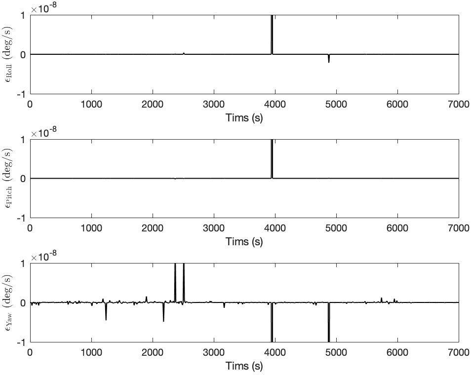
The estimated angular rates from SVD and FS3R are generally the same. Let us define the ’Axis’ difference by

\begin{gathered}\epsilon_{\rm{Axis}}=|\omega_{\rm{Axis,SVD}}-\omega_{\rm{Axis,True}}|-|\omega_{\rm{Axis,FS3R}}-\omega_{\rm{Axis,True}}|\end{gathered}

(27)

where $\rm{Axis}\in\{\rm{Roll,Pitch,Yaw}\}$ and $\omega_{\rm{Axis,True}}$ denotes the true angular rate in the direction of $\rm{Axis}$ obtained from the ground-truth data. We can observe from Fig. 6 that the difference between SVD and proposed FS3R has been enlarged. Here $\epsilon_{\rm{Axis}}>0$ reflects better performance of FS3R, vice versa. In Fig. 6, there are more positive peaks than negative ones, which indicates that here FS3R is slightly more accurate than SVD. Note that the scale of such error is in fact enlarged by mass matching process inside the ICP. Here the root mean-squared (RMS) statistics are summarized in Table V.

TABLE V: RMS results for angular rate estimation from KITTI dataset.

	SVD	Proposed FS3R
$\epsilon_{\rm{Roll}}$	$2.0979\times 10^{-08}\ \rm{deg/s}$	$1.9883\times 10^{-08}\ \rm{deg/s}$
$\epsilon_{\rm{Pitch}}$	$1.9432\times 10^{-08}\ \rm{deg/s}$	$1.8075\times 10^{-08}\ \rm{deg/s}$
$\epsilon_{\rm{Yaw}}$	$3.1302\times 10^{-08}\ \rm{deg/s}$	$2.9963\times 10^{-08}\ \rm{deg/s}$

The shown errors from FS3R are slightly smaller than that from SVD. FS3R can analytically compute the eigenvalue without iterations and thus will not be influenced by numerical thresholds. Therefore the ICP from FS3R may be more applicable on low-configuration platforms. However, we need to point out that here the error scales in Table V can almost be ignored as they have nearly reached the level of nano $\rm{deg/s}$ , which is better than most of expensive fiber-optic gyroscopes. Such requirements may seldom occur in real engineering practices. Thus here the SVD and proposed FS3R can be regarded to own identical accuracy and robustness.

III-D Application Notes

The FS3R, since its invention, has been applied to some time-consuming tasks e.g. point-cloud registration and video stitching. In a recent test where a huge point cloud containing 7889456 points are captured using the Riegl VZ-2000 3D laser scanner on a real-world helicopter (see Fig. 7) for power-line inspection. The original registration method is motivated by the libpointmatcher from ETHZ ASL Lab [26] in which the ICP is completed using the SVD. By replacing SVD with the proposed FS3R, the matching time has been decreased from 1 hour to 0.65 hour. The general results of the point matching are also shown in Fig. 7. The SVD and FS3R in real engineering use have been verified to own the same accuracy and robustness. The huge amount of point correspondences ensure precision estimates of rigid-body transformation. This shows the potential applicability of FS3R in industrial processing. We also have made all the codes in C++ and MATLAB open-source and the audience can verify its effectiveness (see the footnote of the first page).

IV Conclusion

Our recent algorithm FLAE is revisited, which is later related to the 3D registration problem. Some proofs are presented to show the equivalence. The previous solution to quartic equation is then simplified getting rid of complex numbers for easier implementation. Numerical robustness of the proposed method is also investigated showing its immunity to degenerated matrices. The proposed algorithm is systematically evaluated with other representatives. The results indicate that it maintains the accuracy and robustness but consumes much less computation time. Real applications including large-point-cloud registration have shown its superiority in engineering processing. However, it is still noticed that the current method highly relies on the floating-point operations. Unless we have reached the limit of EIG numerical algorithm, we still have an expectation to develop the next-generation algorithm in which the floating-number is no longer need, which, would be of great benefit for parallel computing platforms like FPGA and GPU for accelerated performance.

Acknowledgment

This research was supported by Shenzhen Science, Technology and Innovation Comission (SZSTI) JCYJ20160401100022706, awarded to Prof. Ming Liu., in part by National Natural Science Foundation of China under the grant of No. 41604025, in part by General Research Fund of Research Grants Council Hong Kong,11210017, and also in part by Early Career Scheme Project of Research Grants Council Hong Kong, 21202816 The authors would also like to thank Dr. F. Landis Markley from NASA Goddard Space Flight Center and Prof. Yuanxin Wu from Shanghai Jiao Tong University for their constructive comments to this paper. Dr. Yaguang Yang from Nuclear Research Centre, U.S. Navy provided his codes of [31]. The experimental devices e.g. laser scanner and helicopter are supported by Chongqing Fengmai Innovation Inc., Chongqing, China. We genuinely thank them for their help. The source code of this paper has been uploaded to https://github.com/zarathustr/FS3R (C++), https://github.com/zarathustr/FS3R-Matlab (MATLAB) and https://github.com/zarathustr/FS3R-CrossWorks (Embedded).

References

[1] F. Aghili and C.-Y. Su, “Robust Relative Navigation by Integration of ICP and Adaptive Kalman Filter Using Laser Scanner and IMU,” IEEE/ASME Trans. Mechatronics, vol. 21, no. 4, pp. 1–1, 2016.
[2] L. Wang, M. Liu, and Q. H. Meng, “Real-time multisensor data retrieval for cloud robotic systems,” IEEE Trans. Auto. Sci. Eng., vol. 12, no. 2, pp. 507–518, 2015.
[3] C. Ye, S. Hong, and A. Tamjidi, “6-DOF Pose Estimation of a Robotic Navigation Aid by Tracking Visual and Geometric Features,” IEEE Trans. Auto. Sci. Eng., vol. 12, no. 4, pp. 1169–1180, 2015.
[4] J. Yang and H. Li, “Go-ICP: A Globally Optimal Solution to 3D ICP Point-Set Registration,” IEEE Trans. Pattern Anal. Mach. Intell., vol. 38, no. 11, pp. 2241–2254, 2016.
[5] C. Ye and J. Borenstein, “A Novel Filter for Terrain Mapping With Laser Rangefinders,” IEEE Trans. Robot., vol. 20, no. 5, pp. 913–921, 2004.
[6] T. L. Faber and E. M. Stokely, “Orientation of 3-d structures in medical images,” IEEE Trans. Pattern Anal. Mach. Intell., vol. 10, no. 5, pp. 626–633, 1988.
[7] S. Ying, J. Peng, S. Du, and H. Qiao, “A scale stretch method based on ICP for 3D data registration,” IEEE Trans. Auto. Sci. Eng., vol. 6, no. 3, pp. 559–565, 2009.
[8] Z. Yang and S. Shen, “Monocular Visual-Inertial State Estimation With Online Initialization and Camera-IMU Extrinsic Calibration,” IEEE Trans. Auto. Sci. Eng., vol. 14, no. 1, pp. 39–51, 2016.
[9] M. Liu, “Robotic online path planning on point cloud,” IEEE Trans. Cybern., vol. 46, no. 5, pp. 1217–1228, 2016.
[10] Y. He, B. Liang, J. Yang, S. Li, and J. He, “An Iterative Closest Points Algorithm for Registration of 3D Laser Scanner Point Clouds with Geometric Features,” Sensors, vol. 17, no. 8, p. 1862, 2017.
[11] Z. Zhou, Y. Li, J. Liu, and G. Li, “Equality constrained robust measurement fusion for adaptive kalman-filter-based heterogeneous multi-sensor navigation,” IEEE Trans. Aerosp. Elect. Syst., vol. 49, no. 4, pp. 2146–2157, 2013.
[12] Z. Zhou, Y. Li, J. Zhang, and C. Rizos, “Integrated Navigation System for a Low-Cost Quadrotor Aerial Vehicle in the Presence of Rotor Influences,” J. Survey. Eng., vol. 143, no. 1, p. 05016006, 2017.
[13] K. Kanatani, “Analysis of 3-D Rotation Fitting,” IEEE Trans. Pattern Anal. Mach. Intell., vol. 16, no. 5, pp. 543–549, 1994.
[14] G. Chang, “Total least-squares formulation of Wahba’s problem,” Electron. Lett., vol. 51, no. 17, pp. 1334–1335, 2015.
[15] A. H. J. D. Ruiter and J. Richard, “On the Solution of Wahba’s Problem on SO(n),” J. Astronautical Sci., no. December, pp. 734–763, 2014.
[16] P. J. Besl and N. D. McKay, “A Method for Registration of 3-D Shapes,” IEEE Trans. Pattern Anal. Mach. Intell., vol. 14, no. 2, pp. 239–256, 1992.
[17] V. Govindu and C. Shekhar, “Alignment using distributions of local geometric properties,” IEEE Trans. Pattern Anal. Mach. Intell., vol. 21, no. 10, pp. 1031–1043, 1999.
[18] O. Choi and I. S. Kweon, “Robust feature point matching by preserving local geometric consistency,” Comput. Vis. Image Understand., vol. 113, no. 6, pp. 726–742, 2009.
[19] C. F. Olson, “A general method for geometric feature matching and model extraction,” Int. J. Comput. Vis., vol. 45, no. 1, pp. 39–54, 2001.
[20] J. Zhang, M. Kaess, and S. Singh, “A real-time method for depth enhanced visual odometry,” Autonom. Robot., vol. 41, no. 1, pp. 31–43, 2017.
[21] J. Zhang and S. Singh, “Low-drift and real-time lidar odometry and mapping,” Autonom. Robot., vol. 41, no. 2, pp. 401–416, 2017.
[22] K. S. Arun, T. S. Huang, and S. D. Blostein, “Least-Squares Fitting of Two 3-D Point Sets,” IEEE Trans. Pattern Anal. Mach. Intell., vol. PAMI-9, no. 5, pp. 698–700, 1987.
[23] S. Umeyama, “Least-Squares Estimation of Transformation Parameters Between Two Point Patterns,” IEEE Trans. Pattern Anal. Mach. Intell., vol. 13, no. 4, pp. 376–380, 1991.
[24] M. W. Walker, L. Shao, and R. A. Volz, “Estimating 3-D location parameters using dual number quaternions,” CVGIP: Image Understand., vol. 54, no. 3, pp. 358–367, 1991.
[25] B. K. P. Horn, “Closed-form solution of absolute orientation using unit quaternions,” J. Optic. Soc. America A, vol. 4, no. 4, p. 629, 1987.
[26] F. Pomerleau, F. Colas, R. Siegwart, and S. Magnenat, “Comparing ICP Variants on Real-World Data Sets,” Autonom. Robot., vol. 34, no. 3, pp. 133–148, Feb. 2013.
[27] H. Guo, H. Chen, F. Xu, F. Wang, and G. Lu, “Implementation of EKF for vehicle velocities estimation on FPGA,” IEEE Trans. Indust. Elect., vol. 60, no. 9, pp. 3823–3835, 2013.
[28] J. Wu, Z. Zhou, B. Gao, R. Li, Y. Cheng, and H. Fourati, “Fast Linear Quaternion Attitude Estimator Using Vector Observations,” IEEE Trans. Auto. Sci. Eng., vol. 15, no. 1, pp. 307–319, 2018.
[29] J. Wu, Z. Zhou, H. Fourati, R. Li, and M. Liu, “Generalized Linear Quaternion Complementary Filter for Attitude Estimation from Multi-Sensor Observations : An Optimization Approach,” IEEE Trans. Auto. Sci. Eng., 2019.
[30] Y. Cheng and M. D. Shuster, “Improvement to the Implementation of the QUEST Algorithm,” AIAA J. Guid. Control Dyn., vol. 37, no. 1, pp. 301–305, 2014.
[31] Y. Yang and Z. Zhou, “An analytic solution to Wahbas problem,” Aerosp. Sci. Tech., vol. 30, no. 1, pp. 46–49, 2013.
[32] Z. Liu, W. Liu, X. Gong, and J. Wu, “Optimal attitude determination from vector sensors using fast analytical singular value decomposition,” J. Sensors, 2018.
[33] V. Krishnamurthy and M. Levoy, “Fitting smooth surfaces to dense polygon meshes,” in Proceedings of the 23rd annual conference on Computer graphics and interactive techniques. ACM, 1996, pp. 313–324.
[34] A. Geiger, P. Lenz, and R. Urtasun, “Are we ready for autonomous driving? the kitti vision benchmark suite,” in IEEE CVPR 2012, 2012.
[35] T.-H. Kwok, “Dnss: Dual-normal-space sampling for 3-d icp registration,” IEEE Trans. Auto. Sci. Eng., 2018.
[36] H. Wang, R. Jiang, H. Zhang, and S. S. Ge, “Heading reference-assisted pose estimation for ground vehicles,” IEEE Trans. Auto. Sci. Eng., 2018.