Multi-robot Symmetric Rendezvous Search on the Line
with an Unknown Initial Distance
Abstract
In this paper, we study the symmetric rendezvous search problem on the line with robots that are unaware of their locations and the initial distances between them. In the symmetric version of this problem, the robots execute the same strategy. The multi-robot symmetric rendezvous algorithm, presented in this paper is an extension our symmetric rendezvous algorithm, presented in [22]. We study both the synchronous and asynchronous cases of the problem. The asynchronous version of algorithm is called algorithm. We consider that robots start executing at different times. We perform the theoretical analysis of and and show that their competitive ratios are and , respectively. Finally, we confirm our theoretical results through simulations.
Final International University, North Cyprus, Turkey,
1 Introduction
In the rendezvous search problem, two or more players that are unaware of their locations in the environment and cannot communicate over long distances want to meet as quickly as possible. This problem arises when two people become separated shopping in a mall, when two parachutists who have to meet after a simultaneous landing in a large field, or when rescuers search for a lost hiker who wants to be found. As well as its obvious connection with real life problems, this interesting problem also has various applications in robotic search-and-rescue, network formation, multi-robot exploration and mapping.
In robotic search-and-rescue, rescuers (robots) can search for victims and survivors in urban disasters and explosions. Multiple robots could also be employed to explore and build the map of unknown environments such as mine fields, contaminated areas or distant planets that can be hazardous or inaccessible to humans. To accomplish this task, they might rendezvous to collaboratively explore the environment. Suppose multiple robots are initially employed to perform surveillance in a large environment. Upon detection of an event, they may have to form a network to propagate information as quickly as possible. When robots with limited communication range and different unknown locations are dispersed in a large environment, network formation problem becomes closely related to rendezvous search problems.
The rendezvous search problem has two different versions, depending on whether or not the robots can meet in advance of the search to agree on the strategies each will execute. In asymmetric rendezvous search, the robots can meet in advance and choose distinct strategies. For example, one can wait while the other carries out an exhaustive search. This is different to symmetric rendezvous search, where the robots execute the same strategy, since they do not have chance to agree on their roles. In this version, it is not necessary to implement a different strategy on each robot. Therefore, it is appealing for robotics applications.
Let denote the initial location of robot in an environment and denote the minimum possible distance traveled before rendezvous. The efficiency of a rendezvous strategy is often measured by its competitive ratio
| (1) |
where denotes the (expected) distance traveled by robot before rendezvous. The competitive ratio of is the worst case deviation of the performance of from this optimal behavior. A strategy is said to be competitive if its competitive ratio is a constant.
The contributions of this paper are as follows. We study the symmetric rendezvous search problem with multi-robots on the line for an unknown initial distance. Moreover, the robots do not know their positions or directions. We first present a symmetric rendezvous algorithm for the synchronous setting of the problem. is an extension of our algorithm presented in [22]. We perform the theoretical analysis of and show that its competitive complexity is . Second, we study the problem in the asynchronous setting. For this setting of the problem, is called . We prove that has a competitive complexity of . Finally, we verify the theoretical results that are obtained for both cases in simulations.
The paper is organized as follows. We present an overview of related work in Section 2. algorithm is introduced in Section 3. We formulate the multi-robot rendezvous search problem and present Algorithm in Section 4. In Section 5, we perform the analysis of . We present the asynchronous case of the problem in Section 6 and perform the analysis of this case in Section 7. We present the simulation results in Section 8. Finally, we provide concluding remarks in Section 9.
2 Related Work
The rendezvous search problem can be formulated in various environments such as line, plane, circle(ring) or graph. In this paper, robots are placed on a line with an unknown initial distance between them. A road, a street, a river, a corridor, a railway can me modeled as a line. The rendezvous search problem on the line is studied both for the symmetric [3, 4, 6, 26, 16, 24] and asymmetric [7, 15, 1, 2] versions. Many previous studies focus on the asymmetric version with the players who know their initial distance or its distribution [2, 24]. However, the problem has not been well studied for the symmetric case and unknown initial distance. In the previous version of this paper [22], we present a new symmetric rendezvous algorithm for two robots that has a competitive ratio of 17.686 for total distance traveled and a competitive ratio of 24.843 for total time. Both are improvements over the algorithm of Baston and Gal [7], in which the distance distribution is not known and has a competitive ratio of 26.650. In this paper, we extend our work [22] to multi-robots and provide the theoretical and simulations results for both the synchronous and asynchronous cases of the problem.
Lim et. al [19] studies the rendezvous of blind, speed one, players. The players are placed by a random permutation onto the integers 1 to on the line. Each player points randomly to the right or left, thus have no common notion of a positive direction on the line. The initial distance between each player is known and equal to 1. The least expected rendezvous time of players is given by and for the asymmetric and symmetric strategy, respectively. is 47/48 and is asymptotic to . Prior to this study, Alpern and Lim [18] focus on the asymmetric version of the same problem and minimizing the maximum time to rendezvous rather than the expected time. The asymmetric value of the -player minimax rendezvous time has an upper bound . Gal [15] presents a simpler strategy for the problem in [18] and shows that the worst case meeting time has an asymptotic behavior of .
The asynchronous case of the rendezvous search problem has not received as much attention on the line [20, 24], as in graphs [20, 12, 25, 17, 8, 11, 14] and in geometric environments [5, 10, 11, 13, 9]. We aim to fill this gap in our work. Although [20] concentrates on the asynchronous rendezvous in graphs, the authors also present a deterministic rendezvous algorithm for two agents located on an infinite line. They think of an adversary that interferes the starting times and the motion of an agent. If the agents execute the same deterministic algorithm and the adversary makes them move in the same direction at the same speed, then they will never meet. Thus, the agents have distinct identifiers, called labels. Labels are two different nonempty binary strings, and each agent knows its own label. Based on its label, each agent produces the label . This bit string is a motion pattern which consists of three consecutive segments and is followed by the agent. Because of the asynchronous setting, at the time when agent completes the second segment of the -th bit, agent can be already executing the -th bit. The cost of their algorithm is when is known and when is unknown. Here, and denote the lengths of the shorter and longer label of the agents, respectively. This bound is improved to by Stachowiak [24]. Thomas and Pikounis [25] study the multi-player rendezvous search on a complete graph. The paper focuses on whether players should stick together or split up and meet again later when some but not all of them meet. Authors show that among the class of strategies that require no memory and are stationary, sticking together is the optimal strategy. However, split up and meet again strategy achieves faster expected rendezvous times in most situations.
In the robotics literature, there are two types of rendezvous problems. The first type is interested in robot tracking and navigation toward a moving object (target) where the agents can observe each other’s state. The second type is the rendezvous search problem which we study in this paper. The first type of the problem focuses on the control-theoretic aspects which include combining the kinematics equations of the robot and the target. The target can be another mobile robot, a satellite, a moving convoy or a human. The main difference between these types is that the rendezvous search problem does not use the state information. The robots are not equipped with a (long range) sensory system. Therefore, they cannot determine the position of the other robot to achieve rendezvous. The robots do not necessarily know their current location. Moreover, they do not (and cannot) know the initial distance or direction to the other robot.
3 Preliminaries
In this section, we briefly explain Algorithm. The extension of this algorithm to multi-robots is introduced in Section 4. In the earlier version of the problem, two robots are placed on a line with an with an unknown initial distance between them. The initial distance between the robots is set to , where , for and . To each robot, a non-negative sequence is assigned, where and
Here, is the expansion radius and is a uniformly distributed random variable. The robots use the same expansion radius . They choose their values independently at the start of the algorithm and use them throughout the algorithm. They start executing the algorithm at the same time and continue to synchronize their movements with waiting times.
The algorithm proceeds in rounds indexed by integers . If the robots choose the same direction at the beginning and stick with these directions in later rounds, they will never meet. Thus, randomization is used to break the symmetry between the robots. In round , the robot flips a coin to determine its itinerary. Each round is divided into two phases: phase-1 and phase-2.
We now describe the movement of robot-1, who starts at x = 0. In the th round, the robot starts at one of , each with probability . If the robot tosses heads, then it follows Right-Wait-Left-Wait motion pattern; it moves right to the point in phase-1, waits for some time at the end of this phase, then it moves left to the point and waits for some time at the end of this phase. If the robot tosses tails, then it follows Left-Wait-Right-Wait motion pattern; it moves left to in phase-1, waits for some time at the end of this phase, then moves right to in phase-2 and waits for some time at the end of this phase. A robot determines its waiting time at the end of each phase of a round considering the possible total distance traveled in that phase and assuming that the other robot is using . At the end of an unsuccessful round , the possible configurations of the robots are (). This is also the initial configuration for round .
4 Problem Formulation
In this section, we present the extension of the algorithm to multi-robots. 2 robots are placed on a line with equal initial distances between them. The robots do not know the initial distances between each other. Two robots are adjacent to each other if there is no robot located between them. For example, in Fig. 1, robot-3 is adjacent to both robot-2 and robot-4, and robot-1 is only adjacent to robot-2. As in algorithm , the initial distance between two adjacent robots is set to 2. Robot- is initially located at , where integer . Let the expansion radius 1 be fixed. We determine the choice for in Section 5 for the synchronous case and in Section 7 for the asynchronous case of the problem.

We call the multi-robot version of the algorithm, . Each robot independently executes algorithm without value. Thus, for each robot
When two robots meet in round , they rendezvous into a cluster and the robot with the smaller id becomes the leader of the cluster. The robots inside the cluster thereafter sticks together and follow the motion pattern that is determined by the coin flip of their leader. At the beginning of a round, only the cluster leader flips a coin. Clusters can meet moving towards each other and cannot meet if they move in tandem. More than one cluster can meet in a round.
represents the set of the robots in a cluster which is indexed by with respect to its position from the left on the line. We denote the leader robot in cluster by and the initial location of by . Let be the number of clusters at the beginning of round . in round and decreases by one whenever two clusters meet into a new cluster. At the beginning of round , , thus . Rendezvous occurs in round , when .
Fig. 2 shows sample executions of algorithm when and . In the top and bottom plots, the rendezvous occurs in 6 rounds, while in middle plot, it occurs in 9 rounds. Thus, the robot travels the maximum distance in the middle plot. In simulations (Section 8), we observe that the distance traveled by the robot is proportional to the number of rounds. Given that the rendezvous occurs in round , the distance traveled by the clusters in that round is maximized when Robot-1 and Robot- are the leaders of the last two clusters on the line. Such a case occurs in the second execution of , where robot-1 and robot-6 are the last clusters to meet. We now explain the execution of algorithm shown in the top plot of Fig. 2. Here, Robot-4 and Robot-5 meet in round 3. At the beginning of round 4, the clusters are , , and with the leader robots , , and . In round 5, Robot-1 first meets Robot-2, then Robot-3. At the beginning of round 6, the clusters are and with the leader robots and , respectively. Rendezvous occurs in round 6, when and meet.


5 Analysis of Algorithm
In this section, we analyze the performance of algorithm and find an upper bound on the expected distance traveled by the robot. Note that due to the symmetric strategies, the performance all the robots are the same. For omniscient robots, the best offline algorithm would be for them to move toward each other and meet at . Thus, our competitive ratio will be calculated in comparison with distance .
We denote the probability of a cluster getting a head in one flip of a fair coin by . Let the random variable follow the binomial distribution with parameters and , then the probability of getting exactly heads in coin flips is given by
For and , let , and denote the events , , and in round , respectively. Event
The probability of event is then given by
| if is even, | (2) | ||||
| if is odd. | (3) |
Let be the event that all the robots rendezvous into one cluster in round , i.e., . Assuming that the algorithm is still active in round , let be the event that cluster initially moves to the right and be the event that cluster initially moves to the left in round . Adjacent clusters can meet if event
occurs, and cannot meet if event
occurs. Let and .
In the following lemma, we establish the relation between and .
Lemma 1
For , if heads are obtained in coin flips in round , then decreases by at the end of this round.
Proof
The maximum possible distance between clusters and is given by
| (4) |
At the end of round , is minimized and (4) is maximized when . Therefore, we substitute with in (4) to obtain
| (5) |
Adjacent clusters can only meet if event occurs. That is, if their coin flips are different from each other. The worst-case scenario is defined by the event which occurs when and all heads in the sequence of coin flips appear consecutively. Note that the order of the clusters’ coin flips matters, but the order of clusters’ ids does not matter. We use the clusters’ ids in order only for the ease of representation.
We prove this lemma by showing that decreases by even when event occurs. Given occurs, there is a sequence of events
| (6) |
such that are the only adjacent clusters with different outcomes of coin flips. Therefore, decreases by at the end of round only if meets the next clusters in this sequence. In this case, the distance traveled by the cluster is maximized for . Consider the example sequences of coin flips; H,H,H,H,T,T,T,T, and T,T,T,T,H,H,H,H, where and . Here, decreases by at the end of round only when meets all the clusters in the subsequences T,T,T,T and H,H,H,H in the first and second sequences, respectively. Assuming that event occurs, meets the next clusters in (6), if
| (7) |
Since (7) holds true for and , decreases by .
Although, it seems from (6) like it is enough to have head in round to decrease by , this may not be always true. For example, consider the sequence T,T,T,T,T,T,T,H in round , where . In round , only and can meet. When these clusters stick together in phase-2 of round , we have and . then continues moving right, following the direction of . This results in all the clusters on the line to move in the same direction till the end of this round. Therefore, decreases by .
Lemma 2
For , if heads are obtained in coin flips in round , then decreases by at the end of this round.
Proof
Since , the proof is the same as Lemma 1 when heads are obtained. Therefore, decreases by at the end of this round.
Let denote the event that decreases by at least at the end of round . We say that a round is successful if event occurs in that round, unsuccessful otherwise. From Lemmas 1 and 2, we conclude that if event occurs in round , then event also occurs. Therefore, the probability of round being successful is given by . The minimum number of rounds required for the rendezvous in some round is achieved if occurs in each round . This number is maximized when event occurs and is given by the recursive function
Substituting 11 1 The logarithms in this paper are binary logarithms. into the recurrence yields
| (8) |
Let be the event that the algorithm is still active in round . It follows from (8) that if event occurs less than times in rounds, then event cannot occur, thus . The probability of is given by
| (9) |
Using the finite taylor series polynomial approximation [21], (9) yields
| (10) |
We divide the execution of Algorithm into three stages. Stage-1 consists of rounds that adjacent clusters do not travel far enough to meet. The first round in which the adjacent clusters might meet is round . Stage-2 consists of the rounds . The first round that rendezvous can occur is the (th round. Stage-3 consists of rounds . We now study the three stages of Algorithm for the synchronous case of the problem. Sections 5.1-5.3 present the distance traveled analysis of stages 1-3, respectively.
5.1 Analysis of Stage-1
This section presents the computation of the expected distance traveled during Stage-1.
Lemma 3
The expected distance traveled during Stage-1 satisfies
| (11) |
Proof
Adjacent clusters cannot meet when round . Therefore, in this stage. The possible itineraries of adjacent clusters based on their initial configurations in round are shown in Fig. 3.

The distance traveled (the length of an itinerary) by a cluster in an unsuccessful round is either or , each with equal probability. Therefore, we have
| (12) |
Using (12), we obtain
5.2 Analysis of Stage-2
This section presents the computation of the expected distance traveled during Stage-2 which encompasses the rounds . Adjacent clusters can meet in this stage. However, rendezvous cannot occur until round . Thus, the algorithm is still active during this stage, i.e. .
Lemma 4
The expected distance traveled during Stage-2 satisfies
| (13) |
Proof
The expected distance traveled by a cluster in this stage is given by
5.3 Analysis of Stage-3
We compute the expected distance traveled for all rounds . Unlike Stage-1 and Stage-2, rendezvous occurs in this stage with nonzero probability.
Lemma 5
The expected distance traveled during Stage-3 satisfies
| (14) |
Proof
Given holds, the distance traveled by the clusters is maximized when and where and are the last clusters to rendezvous. Thus, substituting and in (4), we have
| (15) |
In this case, the four equiprobable initial configurations of the clusters are . Thus, the expected distance traveled given holds, is
| (16) |
Comparing and using (12) and (16), respectively, we have
Thus, for the simplicity of subsequent computations, we assume that
The expected distance traveled in Stage-3 is given by
| (17) |
We bound the infinite summation in (17) by
to obtain
Theorem 5.1
For the choice of , algorithm has a competitive ratio of .
Proof
The expected distance traveled is obtained by adding the expressions in equations (11), (13) and (14). Recalling that the initial distance between the adjacent clusters is , where , we first replace each occurrence of with . Then, we divide by which is the length of the optimal offline path between the clusters. This expression is maximized at . In turn, the choice of gives the competitive ratio guarantee of .
6 Algorithm
Until now, we assume that the robots start executing the algorithm at the same time. Although this is a standard assumption, it may often be unrealistic: robots may be created in different parts of the environment modeled as a line, oblivious to each other. Hence, in this section we investigate the symmetric rendezvous of robots that start searching at different times.
Recall that robots wait at the end of each stage of a round to keep their motions synchronized. For the asynchronous setting, we do not use idle times introduced in . The resulting algorithm is called . We consider that robot- starts executing algorithm time late, where is a random integer value drawn from a discrete uniform distribution over the interval . Robots are unaware of each other’s latency.
Proposition 1
Consider two clusters and , where (robot-1) and (robot-2). Assume that these clusters do not meet any other clusters before round . Let . Depending on the values of , , and the coin flips of and , can reach round earlier than despite of its late start.
Proof
Let be the distance traveled by the robot in an unsuccessful round . Since depends on the coin flips of the robot in round and , it can vary among the robots. Without the idle times, total time in round is . In contrast to the algorithm , of the robots in the algorithm can be different from each other. For the following case, we find out the robot that is first to reach round : Consider that none of the outcomes of the two consecutive coin flips of until round are the same. Further consider that all the outcomes of the coin flips of until round are the same. In this case, . If and have values such that the inequality
holds, then arrives round earlier than .
In , the robots do not start each phase of a round at the same time. Therefore, when one robot starts phase-1(2) of round , another robot can be moving in phase-2(1) of the same or another round. Moreover, before the robot reaches its destination in a phase, the other robot can finish its current round, flip a coin to start a new round and change its direction. If adjacent clusters and meet, becomes the leader if is executing a smaller round than . In the next section, we perform the analysis of without the knowledge of .
7 Analysis of the Algorithm
Recall that the initial location of a cluster is . We use the following variables in the analysis: is the time arrives ; is the round that is executing at ; is the round that is executing at . Let .
Lemma 6
If is moving on the left side of at , then the rendezvous has already occurred before .
Proof
Since , if is moving on the left side of when arrives , then should have already met on its way to .
We assume that adjacent clusters cannot meet before . Therefore, we can conclude from Lemma 6 that is in moving on the right of at . Let events - correspond to the events -, respectively, when round for , and for . The possible destinations and of and at are given by the states
that correspond to the events -, respectively. The coin flips of clusters are independent from each other, thus each event occurs with the probability of 1/4. Let . In Lemmas 7-11, we consider that round . We next study the possible rendezvous conditions at .

Lemma 7
Regardless of the value of , adjacent clusters always meet when event occurs.
Proof
Recall that event corresponds to state . We study the the rendezvous behavior of adjacent clusters before on the left side of when is executing phase-1 of round . Thus, we have and . should have flipped head, if its destination is when event occurs. Therefore, when arrives , it starts moving right towards . and always meet when event occurs if
| (18) |
When , (18) is true for the choice of .
Lemma 8
Regardless of the value of , adjacent clusters always meet when event occurs.
Proof
Since corresponds to state , starts moving left towards when it arrives . Thus, and always meet when event occurs if
| (19) |
which is true for and the choice of .
Lemma 9
When , adjacent clusters always meet when event occurs.
Proof
Lemma 10
When , adjacent clusters always meet when event occurs.
Proof
The worst-case scenario when event occurs would be to arrive its destination before , then flip a coin at this position to start round , and start moving right to its new destination . Fig. 4 shows this scenario. In this case, adjacent clusters meet if
| (21) |
(21) with is the same as (19) with . Thus, it is true for the choice of and .
Lemma 11
The probability of for the asynchronous case is the same as the synchronous case of the problem, which is given by .
Proof
Consider that is executing round , which we assume to be the highest round on the line. Let be the set of value between and all the other clusters. Let denote the statement and denote the statement . We study the proof in three cases.
Case (i): The statement is true. In this case, we assume that whenever reaches the initial location of another cluster , . Since , , for . This implies that passes from the initial locations of all the other clusters on the line. From Lemmas 7-10, we prove that when , adjacent clusters can meet in all the possible events -. Therefore, regardless of the value of , always meets at least clusters in round . As a result, .
Case (ii): The statement is true. It implies that whenever reaches the initial location of another cluster , . Since all the clusters on the line are executing the same round, this case is similar to the synchronous case. Thus, we next show that Lemma 1 holds for Case (ii). In Lemmas 7 and 8, we prove that adjacent clusters can meet if event or occurs in round . Moreover, we show that a cluster can travel far enough to meet the next clusters. This completes the proof in Lemma 1. Thus, .
Case (iii): The statement is true. We compare the asynchronous and synchronous cases when there are clusters on the line in both of them. Consider that while all the clusters executing are in round , there is at least one cluster executing in round . We match the coin flips of the same indexed clusters executing and in round . Let be the total number of matches. In round of the synchronous case, heads are obtained in coin flips. Let be the number of heads from heads that appear in matches. We split this case into two subcases: and .
- 1.
Case (iii-a) : From Case (i), we can conclude that in round can meet clusters. Since, , decreases by at least in this case, thus .
- 2.
Case (iii-b) : As shown in Case (i), in round can meet clusters. Moreover, it can be derived from Case (ii) that if heads are obtained in coin flips, decreases by . Therefore, the total number of clusters decreased from clusters at the end of round is . This number is at least , because for Case (iii-b), the inequality holds. Therefore, .
We conclude the proof by showing that in all possible cases above, .
It follows from Lemma 11 that the expected distance calculations in Stages 1-3 for the asynchronous case are analogous to the synchronous calculations except in this case, we use instead of . We summarize the calculations as follows:
Theorem 7.1
For the choice of , algorithm has a competitive ratio of .
Proof
The expected distance traveled is obtained by adding the expressions in equations (22), (23) and (24). We first replace each occurrence of with . Then we divide by which is the length of the optimal offline path between the clusters. This expression is maximized at . In turn, the choice of gives the competitive ratio guarantee of .
8 Simulations
To validate the performance of Algorithms and , we ran a series of simulations varying , , and the starting times. First, we present the simulation results of . Then, we present the simulation results that compare the performances of and , including the effect of navigational errors.
In the left plots of Fig. 5, we investigate the performance of when for various values with respect to the change in . Each pair is averaged over 1000 trials and . The value of is varied between 1.17 and 1.3. The initial distance between each adjacent robot on the line is which is varied between 5 and 50 step sizes. We divide the average distance traveled by to obtain the average distance competitive ratio that is shown in the left-top plot of Fig. 5. The average distance competitive ratio remains constant for most values as changes. We observe that Algorithm performs worse for small values such as and . The left-middle plot in Fig. 5 shows that the average distance traveled by the robots increases as decreases. We observe from left-bottom plot in Fig. 5 that the average number of rounds is proportional to the average distance traveled and increases as decreases.
Next, we investigate the performance of when for various values with respect to the change in . The results are shown in the right plots of Fig. 5. The value of is varied between 1.17 and 1.3, and is varied between 4 and 20. Each pair is averaged over 1000 trials. As expected, the average distance traveled increases as increases. The average number of rounds which is proportional to the average distance traveled also increases as increases and decreases. Recall that . In right-bottom plot, we show the difference between the average number of rounds for rendezvous and . For , the difference is approximately . Thus, rendezvous occurs in rounds which is earlier than the starting round of stage-3 of the analysis.
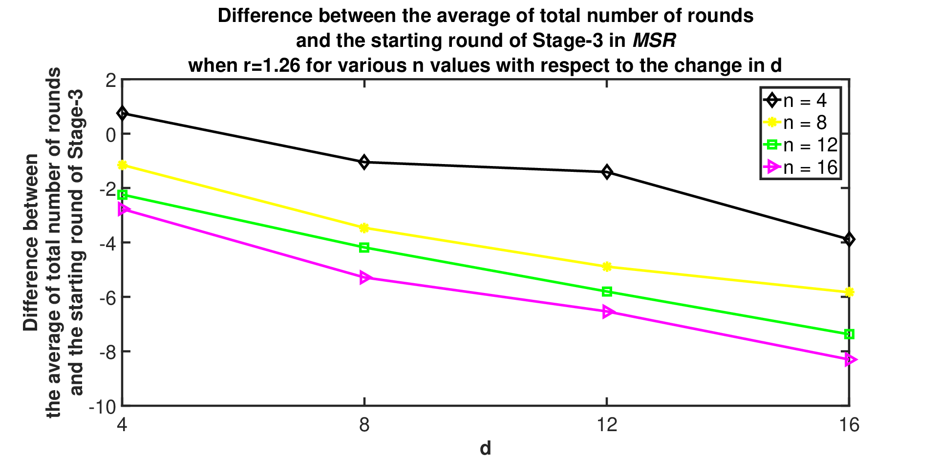
In Fig. 6, we present the simulation results of when both and change. We use the theoretical choice of . The values of and (in terms of step sizes) are varied between 4 and 16. Each pair is averaged over 1000 trials. Top-left plot in Fig. 6 show that the average distance traveled until rendezvous increases as both and increase. Top-right plot in Fig. 6 shows that the average competitive ratio is smaller for , and between 8 and 9. Let denote the round a pair of robots meet for the first time and a new cluster is formed. Let be the total number of rounds required for the rendezvous. Bottom-left plot in Fig. 6 shows the difference between and which is approximately . Let be which is the starting round for Stage-3 introduced in the theoretical analysis. For each pair, we compute the difference between and . The results are shown in bottom-right plot in Fig. 6. We observe that all values except pair are zero or below, implying that the rendezvous occurs at the beginning of Stage-3 or earlier rounds. This verifies the upper bound of which is computed by including the expected distance traveled in Stage-3.
Finally, in Fig.7, we compare the performances of , , and in the presence of navigational errors. Robots start executing time late, where is a uniform random variable generated by robot- on the interval . In addition to the delayed start, the robots do not wait for each other to start the next round or phase of a round. In the literature, the noise caused by navigational errors is often modeled as a Gaussian whose standard deviation is proportional to the distance traveled [23]. We assume that the errors occur only in the -axis while the robots are executing . From Tab. 1 in [23], we use and . Instead of setting , we set , where is the Gaussian noise. As in the theoretical analyses of and , the comparison shown in Fig.7 suggests that robots rendezvous earlier in the synchronous case comparing to the asynchronous case. with gaussian noise performs slightly better than .




9 Conclusion
Unlike most existing work, this paper addresses the multi-robot symmetric rendezvous search problem on the line with an unknown initial distance between the robots. We studied both the synchronous and asynchronous cases of the problem. The algorithms and which are proposed respectively for these cases are an extension of Algorithm presented in [22]. In the synchronous case, robots start executing at the same time and continue to synchronize their movements in later rounds with waiting times. In the asynchronous case, the robots start executing at different times. Waiting times are no longer used in . We showed that the competitive complexity of and are and , respectively. Finally, we verified the theoretical bounds through simulations with respect to the change in , , , and the starting times.
In future work, we will study the multi-robot symmetric rendezvous in graphs. The problem becomes more challenging when the robots do not know the length of the edges which can be the same or varied, also start searching at different times.
References
- (1) Alpern, S., Beck, A.: Asymmetric rendezvous on the line is a double linear search problem. Mathematics of Operations Research 24(3) (1999) 604–618
- (2) Alpern, S., Beck, A.: Pure strategy asymmetric rendezvous on the line with an unknown initial distance. Operations Research 48(3) (2000) 498
- (3) Alpern, S., Gal, S.: Rendezvous search on the line with distinguishable players. SIAM Journal on Control and Optimization 33(4) (1995) 1270–1276
- (4) Anderson, E., Essegaier, S.: Rendezvous search on the line with indistinguishable players. SIAM Journal on Control and Optimization 33 (1995) 1637
- (5) Bampas, E., Czyzowicz, J., Gasieniec, L., Ilcinkas, D., Labourel, A.: Almost optimal asynchronous rendezvous in infinite multidimensional grids. (2010) 297–311
- (6) Baston, V.: Note: Two rendezvous search problems on the line. Naval Research Logistics 46(3) (1999) 335–340
- (7) Baston, V., Gal, S.: Rendezvous on the line when the players’ initial distance is given by an unknown probability distribution. SIAM Journal on Control and Optimization 36 (1998) 1880
- (8) Chalopin, J., Das, S., Santoro, N.: Rendezvous of mobile agents in unknown graphs with faulty links. Distributed Computing (2007) 108–122
- (9) Collins, A., Czyzowicz, J., Gasieniec, L., Labourel, A.: Tell me where i am so i can meet you sooner. (2010) 502–514
- (10) Czyzowicz, J., Ilcinkas, D., Labourel, A., Pelc, A.: Asynchronous deterministic rendezvous in bounded terrains. Structural Information and Communication Complexity (2010) 72–85
- (11) Czyzowicz, J., Labourel, A., Pelc, A.: How to meet asynchronously (almost) everywhere. Arxiv preprint arXiv:1001.0890 (2010)
- (12) Dessmark, A., Fraigniaud, P., Kowalski, D., Pelc, A.: Deterministic rendezvous in graphs. Algorithmica 46(1) (2006) 69–96
- (13) Dieudonné, Y., Pelc, A.: Price of asynchrony in mobile agents computing. Theoretical Computer Science 524 (2014) 59–67
- (14) Dieudonné, Y., Pelc, A., Villain, V.: How to meet asynchronously at polynomial cost. In: Proceedings of the 2013 ACM symposium on Principles of distributed computing, ACM (2013) 92–99
- (15) Gal, S.: Rendezvous search on the line. Operations Research (1999) 974–976
- (16) Han, Q., Du, D., Vera, J., Zuluaga, L.: Improved bounds for the symmetric rendezvous value on the line. In: Proceedings of the eighteenth annual ACM-SIAM symposium on Discrete algorithms, Society for Industrial and Applied Mathematics (2007) 78
- (17) Kowalski, D., Pelc, A.: Polynomial deterministic rendezvous in arbitrary graphs. Algorithms and Computation (2005) 644–656
- (18) Lim, W.S., Alpern, S.: Minimax rendezvous on the line. SIAM Journal on Control and Optimization 34(5) (1996) 1650–1665
- (19) Lim, W., Alpern, S., Beck, A.: Rendezvous search on the line with more than two players. Operations Research 45(3) (1997) 357–364
- (20) Marco, G., Gargano, L., Kranakis, E., Krizanc, D., Pelc, A., Vaccaro, U.: Asynchronous deterministic rendezvous in graphs. Theoretical Computer Science 355(3) (2006) 315–326
- (21) Olson, L.: Lecture notes on taylor series: Expansions, approximations and error (2015)
- (22) Ozsoyeller, D., Beveridge, A., Isler, V.: Symmetric rendezvous search on the line with an unknown initial distance. IEEE Transactions on Robotics 29(6) (2013) 1366–1379
- (23) Rekleitis, I.: A particle filter tutorial for mobile robot localization. Technical Report CIM-04-02, McGill University (2004)
- (24) Stachowiak, G.: Asynchronous Deterministic Rendezvous on the Line. SOFSEM 2009: Theory and Practice of Computer Science (2009) 497–508
- (25) Thomas, L., Pikounis, M.: Many-player rendezvous search: Stick together or split and meet? Naval Research Logistics 48(8) (2001) 710–721
- (26) Uthaisombut, P.: Symmetric rendezvous search on the line using move patterns with different lengths (2006)