跳到论文正文
W Papers独立论文阅读器 arXiv:1805.08606 论文正文 计算阅读时间 · 0%
引用这篇论文根据当前论文元数据生成,正式投稿前建议核对。


License: arXiv.org perpetual non-exclusive license
arXiv:1805.08606v3 [cs.LO] 20 Feb 2024

A set-based reasoner for the description logic \mathcal​D​L𝐃4,×\mathcal{DL}_{\mathbf{D}}^{4,\!\times} (Extended Version)

Domenico Cantone    Marianna Nicolosi-Asmundo    Daniele Francesco Santamaria Affiliation: University of Catania, Dept. of Mathematics and Computer Science
 email: {cantone,nicolosi,santamaria}@dmi.unict.it
Abstract

We present a KE-tableau-based implementation of a reasoner for a decidable fragment of (stratified) set theory expressing the description logic \mathcal​D​L​⟨𝟦​𝖫​𝖰​𝖲𝖱,×⟩​(𝐃)\mathcal{DL}\langle\mathsf{4LQS^{R,\!\times}}\rangle(\mathbf{D}) (\mathcal​D​L𝐃4,×\mathcal{DL}_{\mathbf{D}}^{4,\!\times}, for short). Our application solves the main TBox and ABox reasoning problems for \mathcal​D​L𝐃4,×\mathcal{DL}_{\mathbf{D}}^{4,\!\times}. In particular, it solves the consistency problem for \mathcal​D​L𝐃4,×\mathcal{DL}_{\mathbf{D}}^{4,\!\times}-knowledge bases represented in set-theoretic terms, and a generalization of the Conjunctive Query Answering problem in which conjunctive queries with variables of three sorts are admitted. The reasoner, which extends and optimizes a previous prototype for the consistency checking of \mathcal​D​L𝐃4,×\mathcal{DL}_{\mathbf{D}}^{4,\!\times}-knowledge bases (see [7]), is implemented in C++. It supports \mathcal​D​L𝐃4,×\mathcal{DL}_{\mathbf{D}}^{4,\!\times}-knowledge bases serialized in the OWL/XML format, and it admits also rules expressed in SWRL (Semantic Web Rule Language).

1 Introduction

A wealth of decidability results has been collected over the years within the research field of Computable Set Theory [2, 10, 16]. However, only recently some of these results have been applied in the context of knowledge representation and reasoning for the semantic web. Such efforts have been motivated by the characteristics of the set-theoretic fragments considered, as they provide very expressive unique formalisms that combine the modelling capabilities of a rule language with the constructs of description logics. The decidable multi-sorted quantified set-theoretic fragment 𝟦​𝖫​𝖰​𝖲𝖱\mathsf{4LQS^{R}} [3] is appropriate in this sense, in consideration of the fact that its decision procedure is efficiently implementable. We recall that the language of 𝟦​𝖫​𝖰​𝖲𝖱\mathsf{4LQS^{R}} involves variables of four sorts, pair terms, and a restricted form of quantification.

In [5], the theory 𝟦​𝖫​𝖰​𝖲𝖱\mathsf{4LQS^{R}} has been used to represent the expressive description logic \mathcal​D​L𝐃4,×\mathcal{DL}_{\mathbf{D}}^{4,\!\times} by means of a suitable translation mapping. Moreover, decidability of the most widespread reasoning problems for \mathcal​D​L𝐃4,×\mathcal{DL}_{\mathbf{D}}^{4,\!\times}, such as the consistency problem and the Conjunctive Query Answering (CQA) problem for \mathcal​D​L𝐃4,×\mathcal{DL}_{\mathbf{D}}^{4,\!\times}-knowledge bases (KBs) were proved via a reduction to the satisfiability problem for 𝟦​𝖫​𝖰​𝖲𝖱\mathsf{4LQS^{R}}. Since 𝟦​𝖫​𝖰​𝖲𝖱\mathsf{4LQS^{R}} admits variables of four sorts, the CQA problem was generalized in such a way as to admit queries over three sorts of variables. Such a generalization, called Higher-Order Conjunctive Query Answering (HOCQA) problem can be instantiated to the most widespread reasoning tasks for \mathcal​D​L𝐃4,×\mathcal{DL}_{\mathbf{D}}^{4,\!\times}-ABox.

The description logic \mathcal​D​L𝐃4,×\mathcal{DL}_{\mathbf{D}}^{4,\!\times} admits Boolean operators on concepts and abstract roles, concept domain and range, and existential and minimum cardinality restriction on the left-hand side of inclusion axioms. It also supports role chains on the left-hand side of inclusion axioms and properties on roles such as transitivity, symmetry, and reflexivity. In [4], its consistency problem has been shown to be NP-complete under not very restrictive constraints. Such a low complexity result depends on the fact that existential quantification cannot appear on the right-hand side of inclusion axioms. Nonetheless, \mathcal​D​L𝐃4,×\mathcal{DL}_{\mathbf{D}}^{4,\!\times} turns out to be more expressive than other low complexity logics such as OWL RL [15] and therefore it is very suitable for representing real-world ontologies. For instance, the restricted version of \mathcal​D​L𝐃4,×\mathcal{DL}_{\mathbf{D}}^{4,\!\times} mentioned above allows one to express several OWL ontologies, such as ArcheOntology [15] and OntoCeramic [9], for the classification of archaeological finds, and ArchivioMuseoFabbrica [1], concerning the renovation of the Monastery of San Nicola l’Arena in Catania by the architect Giancarlo De Carlo. Since existential quantification is admitted only on the left-hand side of inclusion axioms, \mathcal​D​L𝐃4,×\mathcal{DL}_{\mathbf{D}}^{4,\!\times} is less expressive than logics such as \mathcal​S​R​O​I​Q​(𝐃)\mathcal{SROIQ}(\mathbf{D}) [12] as long as the generation of new individuals is concerned. On the other hand, \mathcal​D​L𝐃4,×\mathcal{DL}_{\mathbf{D}}^{4,\!\times} is more liberal than \mathcal​S​R​O​I​Q​(𝐃)\mathcal{SROIQ}(\mathbf{D}) in the definition of role inclusion axioms, as the roles involved in \mathcal​D​L𝐃4,×\mathcal{DL}_{\mathbf{D}}^{4,\!\times} are not subject to any ordering relationship, and the notion of simple role is not needed. For example, the role hierarchy presented in [12, page 2] is not expressible in \mathcal​S​R​O​I​Q​(𝐃)\mathcal{SROIQ}(\mathbf{D}), but can be represented in \mathcal​D​L𝐃4,×\mathcal{DL}_{\mathbf{D}}^{4,\!\times}. In addition, \mathcal​D​L𝐃4,×\mathcal{DL}_{\mathbf{D}}^{4,\!\times} is a powerful rule language able to express rules with negated atoms such as

𝑃𝑒𝑟𝑠𝑜𝑛⁡(?​p)∧¬ℎ𝑎𝑠𝐻𝑜𝑚𝑒⁡(?​p,?​h)⟹𝐻𝑜𝑚𝑒𝑙𝑒𝑠𝑠𝑃𝑒𝑟𝑠𝑜𝑛⁡(?​p)\mathit{Person}(?p)\wedge\neg\mathit{hasHome}(?p,?h)\implies\mathit{HomelessPerson}(?p)

that are not supported by the SWRL language.

In [7], we presented a first effort to implement in C++ a KE-tableau-based decision procedure for the consistency problem of \mathcal​D​L𝐃4,×\mathcal{DL}_{\mathbf{D}}^{4,\!\times}-KBs, by resorting to the algorithm introduced in [5]. The choice of KE-tableau systems [13], instead of traditional semantic tableaux [18], was motivated by the fact that KE-tableau systems introduce an analytic cut rule which permits to construct trees whose branches define mutually exclusive situations, thus avoiding the proliferation of redundant branches, typical of Smullyan’s semantic tableaux [18]. Thus, given as input a consistent KB, the procedure yields a KE-tableau whose open branches induce distinct models of the KB. Otherwise, a closed KE-tableau is returned.

In this contribution we improve the reasoner presented in [7] by introducing a system called KEγ-tableau which admits a generalization of the KE-elimination rule incorporating the γ\gamma-rule, namely the expansion rule for handling universally quantified formulae. The reasoner also includes a procedure to compute the HOCQA problem for \mathcal​D​L𝐃4,×\mathcal{DL}_{\mathbf{D}}^{4,\!\times}. Finally, through suitable benchmark tests, we show that such a novel reasoner is more efficient than the one introduced in [7].

2 Preliminaries

2.1 The set-theoretic fragment

We summarize the set-theoretic notions underpinning the description logic \mathcal​D​L𝐃4,×\mathcal{DL}_{\mathbf{D}}^{4,\!\times} and its reasoning tasks. For the sake of conciseness, we avoid to report here the syntax and semantics of the whole 𝟦​𝖫​𝖰​𝖲𝖱\mathsf{4LQS^{R}} theory (the interested reader can find it in [3] together with the decision procedure for its satisfiability problem). Thus, we focus on the 𝟦​𝖫​𝖰​𝖲𝖱\mathsf{4LQS^{R}}-formulae de facto involved in the set-theoretic representation of \mathcal​D​L𝐃4,×\mathcal{DL}_{\mathbf{D}}^{4,\!\times}, namely propositional combinations of 𝟦​𝖫​𝖰​𝖲𝖱\mathsf{4LQS^{R}}-literals (atomic formulae or their negations) and 𝟦​𝖫​𝖰​𝖲𝖱\mathsf{4LQS^{R}} purely universal formulae of the types displayed in Table 1. The class of such 𝟦​𝖫​𝖰​𝖲𝖱\mathsf{4LQS^{R}}-formulae is called 𝟦​𝖫​𝖰​𝖲\mathcal​D​LD4,​×𝖱\mathsf{4LQS}_{\scriptscriptstyle{\mathcal{DL}_{\lx@scalerel@obj{\mathbf{D}}}^{\lx@scalerel@obj{4,\!\times}}}}^{\mathsf{R}}.

We recall that the fragment 𝟦​𝖫​𝖰​𝖲𝖱\mathsf{4LQS^{R}} admits four collections, 𝚅𝚊𝚛i\mathtt{Var}_{i}, of variables of sort ii denoted by Xi,Yi,Zi,…X^{i},Y^{i},Z^{i},\ldots, for i=0,1,2,3i=0,1,2,3 (variables of sort 00 are also denoted by x,y,z,…x,y,z,\ldots). Besides variables, also pair terms of the form ⟨x,y⟩\langle x,y\rangle, with x,y∈𝚅𝚊𝚛0x,y\in\mathtt{Var}_{0}, are allowed. Since the types of formulae displayed in Table 1 do not contain variables of sort 22, here we limit ourselves only to notions and definitions relative to 𝟦​𝖫​𝖰​𝖲\mathcal​D​LD4,​×𝖱\mathsf{4LQS}_{\scriptscriptstyle{\mathcal{DL}_{\lx@scalerel@obj{\mathbf{D}}}^{\lx@scalerel@obj{4,\!\times}}}}^{\mathsf{R}}-formulae involving variables of sorts 0,1,0,1, and 33.

Literals of level 0 Purely universal quantified formulae of level 1
x=y,x∈X1,⟨x,y⟩∈X3x=y,\;x\in X^{1},\;\langle x,y\rangle\in X^{3} (∀z1)​…​(∀zn)​φ0(\forall z_{1})\ldots(\forall z_{n})\varphi_{0}, where z1,…,zn∈𝚅𝚊𝚛0z_{1},\ldots,z_{n}\in\mathtt{Var}_{0} and φ0\varphi_{0} is any propositional combination of literals of level 0.
¬(x=y),¬(x∈X1),¬(⟨x,y⟩∈X3)\neg(x=y),\;\neg(x\in X^{1}),\;\neg(\langle x,y\rangle\in X^{3})
Table 1: Types of literals and quantified formulae admitted in 𝟦​𝖫​𝖰​𝖲\mathcal​D​LD4,​×𝖱\mathsf{4LQS}_{\scriptscriptstyle{\mathcal{DL}_{\lx@scalerel@obj{\mathbf{D}}}^{\lx@scalerel@obj{4,\!\times}}}}^{\mathsf{R}}.

The variables z1,…,znz_{1},\ldots,z_{n} are said to occur quantified in (∀z1)​…​(∀zn)​φ0(\forall z_{1})\ldots(\forall z_{n})\varphi_{0}. A variable occurs free in a 𝟦​𝖫​𝖰​𝖲\mathcal​D​LD4,​×𝖱\mathsf{4LQS}_{\scriptscriptstyle{\mathcal{DL}_{\lx@scalerel@obj{\mathbf{D}}}^{\lx@scalerel@obj{4,\!\times}}}}^{\mathsf{R}}-formula φ\varphi if it does not occur quantified in any subformula of φ\varphi. For i=0,1,3i=0,1,3, we denote with 𝚅𝚊𝚛i​(φ)\mathtt{Var}_{i}(\varphi) the collections of variables of sort ii occurring free in φ\varphi.

Given sequences of distinct variables x→\vec{x} (in 𝚅𝚊𝚛0\mathtt{Var}_{0}), X→1\vec{X}^{1} (in 𝚅𝚊𝚛1\mathtt{Var}_{1}), and X→3\vec{X}^{3} (in 𝚅𝚊𝚛3\mathtt{Var}_{3}), of length nn, mm, and qq, respectively, and sequences of (not necessarily distinct) variables y→\vec{y} (in 𝚅𝚊𝚛0\mathtt{Var}_{0}), Y→1\vec{Y}^{1} (in 𝚅𝚊𝚛1\mathtt{Var}_{1}), and Y→3\vec{Y}^{3} (in 𝚅𝚊𝚛3\mathtt{Var}_{3}), also of length nn, mm, and qq, respectively, the 𝟦​𝖫​𝖰​𝖲\mathcal​D​LD4,​×𝖱\mathsf{4LQS}_{\scriptscriptstyle{\mathcal{DL}_{\lx@scalerel@obj{\mathbf{D}}}^{\lx@scalerel@obj{4,\!\times}}}}^{\mathsf{R}}-substitution σ≔{x→/y→,X→1/Y→1,X→3/Y→3}\sigma\coloneqq\{\vec{x}/\vec{y},\vec{X}^{1}/\vec{Y}^{1},\vec{X}^{3}/\vec{Y}^{3}\} is the mapping φ↦φ​σ\varphi\mapsto\varphi\sigma such that, for any given universal quantified 𝟦​𝖫​𝖰​𝖲\mathcal​D​LD4,​×𝖱\mathsf{4LQS}_{\scriptscriptstyle{\mathcal{DL}_{\lx@scalerel@obj{\mathbf{D}}}^{\lx@scalerel@obj{4,\!\times}}}}^{\mathsf{R}}-formula φ\varphi, φ​σ\varphi\sigma is the result of replacing in φ\varphi the free occurrences of the variables xix_{i} in x→\vec{x} (for i=1,…,ni=1,\ldots,n) with the corresponding yiy_{i} in y→\vec{y}, of Xj1X^{1}_{j} in X→1\vec{X}^{1} (for j=1,…,mj=1,\ldots,m) with Yj1Y^{1}_{j} in Y→1\vec{Y}^{1}, and of Xh3X^{3}_{h} in X→3\vec{X}^{3} (for h=1,…,qh=1,\ldots,q) with Yh3Y^{3}_{h} in Y→3\vec{Y}^{3}, respectively. A substitution σ\sigma is free for φ\varphi if the formulae φ\varphi and φ​σ\varphi\sigma have exactly the same occurrences of quantified variables. The empty substitution, denoted ϵ\epsilon, satisfies φ​ϵ=φ\varphi\epsilon=\varphi, for each 𝟦​𝖫​𝖰​𝖲\mathcal​D​LD4,​×𝖱\mathsf{4LQS}_{\scriptscriptstyle{\mathcal{DL}_{\lx@scalerel@obj{\mathbf{D}}}^{\lx@scalerel@obj{4,\!\times}}}}^{\mathsf{R}}-formula φ\varphi.

A 𝟦​𝖫​𝖰​𝖲\mathcal​D​LD4,​×𝖱\mathsf{4LQS}_{\scriptscriptstyle{\mathcal{DL}_{\lx@scalerel@obj{\mathbf{D}}}^{\lx@scalerel@obj{4,\!\times}}}}^{\mathsf{R}}-interpretation is a pair ℳ=(𝒟,ℳ)\mathbfcal{M}=(D,M), where DD is a nonempty collection of objects (called domain or universe of ℳ\mathbfcal{M}) and MM is an assignment over the variables in 𝚅𝚊𝚛i\mathtt{Var}_{i}, for i=0,1,3i=0,1,3, such that:

M​X0∈D,M​X1∈\mathcal​P​(D),M​X3∈\mathcal​P​(\mathcal​P​(\mathcal​P​(D))),MX^{0}\in D,MX^{1}\in\mathcal{P}(D),MX^{3}\in\mathcal{P}(\mathcal{P}(\mathcal{P}(D))),

where Xi∈𝚅𝚊𝚛iX^{i}\in\mathtt{Var}_{i}, for i=0,1,3i=0,1,3, and \mathcal​P​(s)\mathcal{P}(s) denotes the powerset of ss.

Pair terms are interpreted à la Kuratowski, and therefore we put

M⁡⟨x,y⟩≔{{M​x},{M​x,M​y}}M\langle x,y\rangle\coloneqq\{\{Mx\},\{Mx,My\}\}.

Next, let

  • -

    ℳ=(𝒟,ℳ)\mathbfcal{M}=(D,M) be a 𝟦​𝖫​𝖰​𝖲\mathcal​D​LD4,​×𝖱\mathsf{4LQS}_{\scriptscriptstyle{\mathcal{DL}_{\lx@scalerel@obj{\mathbf{D}}}^{\lx@scalerel@obj{4,\!\times}}}}^{\mathsf{R}}-interpretation,

  • -

    x1,…,xn∈𝚅𝚊𝚛0x_{1},\ldots,x_{n}\in\mathtt{Var}_{0}, and

  • -

    u1,…,un∈Du_{1},\ldots,u_{n}\in D.

By ℳ⁡[§→/⊓→]\mathbfcal{M}[\vec{x}/\vec{u}], we denote the interpretation ℳ′=(𝒟,ℳ′)\mathbfcal{M}^{\prime}=(D,M^{\prime}) such that M′​xi=uiM^{\prime}x_{i}=u_{i} (for i=1,…,ni=1,\ldots,n), and which otherwise coincides with MM on all remaining variables. For a 𝟦​𝖫​𝖰​𝖲\mathcal​D​LD4,​×𝖱\mathsf{4LQS}_{\scriptscriptstyle{\mathcal{DL}_{\lx@scalerel@obj{\mathbf{D}}}^{\lx@scalerel@obj{4,\!\times}}}}^{\mathsf{R}}-interpretation ℳ=(𝒟,ℳ)\mathbfcal{M}=(D,M) and a formula φ\varphi, the satisfiability relationship ℳ⊧φ\mathbfcal{M}\models\varphi is recursively defined over the structure of φ\varphi as follows. Literals are evaluated in a standard way, based on the usual interpretation of the predicates ‘∈\in’ and ‘==’, and of the propositional negation ‘¬\neg’. Compound formulae are interpreted according to the standard rules of propositional logic. Finally, purely universal formulae are evaluated as follows:

  • -

    ℳ⊧(∀‡∞)…(∀‡\)φ′\mathbfcal{M}\models(\forall z_{1})\ldots(\forall z_{n})\varphi_{0} iff ℳ⁡[‡→/⊓→]⊧φ′\mathbfcal{M}[\vec{z}/\vec{u}]\models\varphi_{0}, for all u→∈Dn\vec{u}\in D^{n}.

If ℳ⊧φ\mathbfcal{M}\models\varphi, then ℳ\mathbfcal{M} is said to be a 𝟦​𝖫​𝖰​𝖲\mathcal​D​LD4,​×𝖱\mathsf{4LQS}_{\scriptscriptstyle{\mathcal{DL}_{\lx@scalerel@obj{\mathbf{D}}}^{\lx@scalerel@obj{4,\!\times}}}}^{\mathsf{R}}-model for φ\varphi. A 𝟦​𝖫​𝖰​𝖲\mathcal​D​LD4,​×𝖱\mathsf{4LQS}_{\scriptscriptstyle{\mathcal{DL}_{\lx@scalerel@obj{\mathbf{D}}}^{\lx@scalerel@obj{4,\!\times}}}}^{\mathsf{R}}-formula is said to be satisfiable if it has a 𝟦​𝖫​𝖰​𝖲\mathcal​D​LD4,​×𝖱\mathsf{4LQS}_{\scriptscriptstyle{\mathcal{DL}_{\lx@scalerel@obj{\mathbf{D}}}^{\lx@scalerel@obj{4,\!\times}}}}^{\mathsf{R}}-model. A 𝟦​𝖫​𝖰​𝖲\mathcal​D​LD4,​×𝖱\mathsf{4LQS}_{\scriptscriptstyle{\mathcal{DL}_{\lx@scalerel@obj{\mathbf{D}}}^{\lx@scalerel@obj{4,\!\times}}}}^{\mathsf{R}}-formula is valid if it is satisfied by all 𝟦​𝖫​𝖰​𝖲\mathcal​D​LD4,​×𝖱\mathsf{4LQS}_{\scriptscriptstyle{\mathcal{DL}_{\lx@scalerel@obj{\mathbf{D}}}^{\lx@scalerel@obj{4,\!\times}}}}^{\mathsf{R}}-interpretations.

2.2 The logic \mathcal​D​L​⟨𝟦​𝖫​𝖰​𝖲𝖱,×⟩​(𝐃)\mathcal{DL}\langle\mathsf{4LQS^{R,\!\times}}\rangle(\mathbf{D})

It is convenient to recall the main notions and definitions concerning the description logic \mathcal​D​L​⟨𝟦​𝖫​𝖰​𝖲𝖱,×⟩​(𝐃)\mathcal{DL}\langle\mathsf{4LQS^{R,\!\times}}\rangle(\mathbf{D}) (also called \mathcal​D​L𝐃4,×\mathcal{DL}_{\mathbf{D}}^{4,\!\times}) [4].

Let 𝐑𝐀\mathbf{R_{A}}, 𝐑𝐃\mathbf{R_{D}}, 𝐂\mathbf{C}, and 𝐈𝐧𝐝\mathbf{Ind} be denumerable pairwise disjoint sets of abstract role names, concrete role names, concept names, and individual names, respectively. We assume that the set of abstract role names 𝐑𝐀\mathbf{R_{A}} contains a name UU denoting the universal role.

Data types are introduced through the notion of data type maps, defined according to [14] as follows. A data type map is a quadruple 𝐃=(ND,NC,NF,⋅𝐃)\mathbf{D}=(N_{D},N_{C},N_{F},\cdot^{\mathbf{D}}), where NDN_{D} is a finite set of data types, NCN_{C} is a function assigning a set of constants NC​(d)N_{C}(d) to each data type d∈NDd\in N_{D}, NFN_{F} is a function assigning a set of facets NF​(d)N_{F}(d) to each d∈NDd\in N_{D}, and ⋅𝐃\cdot^{\mathbf{D}} is (i) a function assigning a data type interpretation d𝐃d^{\mathbf{D}} to each data type d∈NDd\in N_{D}, (ii) a facet interpretation f𝐃⊆d𝐃f^{\mathbf{D}}\subseteq d^{\mathbf{D}} to each facet f∈NF​(d)f\in N_{F}(d), and (iii) a data value ed𝐃∈d𝐃e_{d}^{\mathbf{D}}\in d^{\mathbf{D}} to every constant ed∈NC​(d)e_{d}\in N_{C}(d). Facets determine subsets of data values considered of interest in a specific application domain. We shall assume that the interpretations of the data types in NDN_{D} are nonempty pairwise disjoint sets.

(a) \mathcal​D​L𝐃4,×\mathcal{DL}_{\mathbf{D}}^{4,\!\times}-data types, (b) \mathcal​D​L𝐃4,×\mathcal{DL}_{\mathbf{D}}^{4,\!\times}-concepts, (c) \mathcal​D​L𝐃4,×\mathcal{DL}_{\mathbf{D}}^{4,\!\times}-abstract roles, and (d) \mathcal​D​L𝐃4,×\mathcal{DL}_{\mathbf{D}}^{4,\!\times}-concrete role terms are defined according to the DL standard notation (see [12]) as follows:

  • (a)

    t1,t2⟶d​r​|¬t1|​t1⊓t2​|t1⊔t2|​{ed},t_{1},t_{2}\longrightarrow dr~|~\neg t_{1}~|~t_{1}\sqcap t_{2}~|~t_{1}\sqcup t_{2}~|~\{e_{d}\}\,,

  • (b)

    C1,C2⟶A|⊤|⊥|¬C1|C1⊔C2|C1⊓C2|{a}|∃R.𝑆𝑒𝑙𝑓|∃R.{a}|∃P.{ed},C_{1},C_{2}\longrightarrow A~|~\top~|~\bot~|~\neg C_{1}~|~C_{1}\sqcup C_{2}~|~C_{1}\sqcap C_{2}~|~\{a\}~|~\exists R.\mathit{Self}|\exists R.\{a\}|\exists P.\{e_{d}\}\,,

  • (c)

    R1,R2⟶S|U|R1−|¬R1|R1⊔R2|R1⊓R2|RC1||R|C1|RC1|C2|id(C)|R_{1},R_{2}\longrightarrow S~|~U~|~R_{1}^{-}~|~\neg R_{1}~|~R_{1}\sqcup R_{2}~|~R_{1}\sqcap R_{2}~|~R_{C_{1}|}~|~R_{|C_{1}}~|~R_{C_{1}~|~C_{2}}~|~id(C)~|~

    C1×C2,C_{1}\times C_{2}\,,

  • (d)

    P1,P2⟶T|¬P1|P1⊔P2|P1⊓P2|PC1||P|t1|PC1|t1,P_{1},P_{2}\longrightarrow T~|~\neg P_{1}~|~P_{1}\sqcup P_{2}~|~P_{1}\sqcap P_{2}~|~P_{C_{1}|}~|~P_{|t_{1}}~|~P_{C_{1}|t_{1}}\,,

where d​rdr is a data range for 𝐃\mathbf{D}, t1,t2t_{1},t_{2} are data type terms, ede_{d} is a constant in NC​(d)N_{C}(d), aa is an individual name, AA is a concept name, C1,C2C_{1},C_{2} are \mathcal​D​L𝐃4,×\mathcal{DL}_{\mathbf{D}}^{4,\!\times}-concept terms, SS is an abstract role name, R,R1,R2R,R_{1},R_{2} are \mathcal​D​L𝐃4,×\mathcal{DL}_{\mathbf{D}}^{4,\!\times}-abstract role terms, TT is a concrete role name, and P,P1,P2P,P_{1},P_{2} are \mathcal​D​L𝐃4,×\mathcal{DL}_{\mathbf{D}}^{4,\!\times}-concrete role terms. Notice that data type terms are intended to represent derived data types.

A \mathcal​D​L𝐃4,×\mathcal{DL}_{\mathbf{D}}^{4,\!\times}-KB is a triple \mathcal​K=(\mathcal​R,\mathcal​T,\mathcal​A){\mathcal K}=(\mathcal{R},\mathcal{T},\mathcal{A}) such that \mathcal​R\mathcal{R} is a \mathcal​D​L𝐃4,×\mathcal{DL}_{\mathbf{D}}^{4,\!\times}-RBox, \mathcal​T\mathcal{T} is a \mathcal​D​L𝐃4,×\mathcal{DL}_{\mathbf{D}}^{4,\!\times}-TBox, and \mathcal​A\mathcal{A} a \mathcal​D​L𝐃4,×\mathcal{DL}_{\mathbf{D}}^{4,\!\times}-ABox.

A \mathcal​D​L𝐃4,×\mathcal{DL}_{\mathbf{D}}^{4,\!\times}-R​B​o​xRBox is a collection of statements of the following types:

R1≡R2,R1⊑R2,R1​…​Rn⊑Rn+1,𝖲𝗒𝗆⁡(R1),𝖠𝗌𝗒𝗆⁡(R1),𝖱𝖾𝖿⁡(R1),𝖨𝗋𝗋𝖾𝖿⁡(R1),𝖣𝗂𝗌⁡(R1,R2),𝖳𝗋𝖺⁡(R1),𝖥𝗎𝗇⁡(R1),R1≡C1×C2,P1≡P2,P1⊑P2,𝖣𝗂𝗌⁡(P1,P2),𝖥𝗎𝗇⁡(P1),\begin{array}[]{cccccccccc}R_{1}\equiv R_{2},&R_{1}\sqsubseteq R_{2},&~~R_{1}\ldots R_{n}\sqsubseteq R_{n+1},&\mathsf{Sym}(R_{1}),&\mathsf{Asym}(R_{1}),\\ \mathsf{Ref}(R_{1}),&\mathsf{Irref}(R_{1}),&\mathsf{Dis}(R_{1},R_{2}),&\mathsf{Tra}(R_{1}),&\mathsf{Fun}(R_{1}),\\ R_{1}\equiv C_{1}\times C_{2},&P_{1}\equiv P_{2},&P_{1}\sqsubseteq P_{2},&\mathsf{Dis}(P_{1},P_{2}),&\mathsf{Fun}(P_{1}),\end{array}

where R1,R2R_{1},R_{2} are \mathcal​D​L𝐃4,×\mathcal{DL}_{\mathbf{D}}^{4,\!\times}-abstract role terms, C1,C2C_{1},C_{2} are \mathcal​D​L𝐃4,×\mathcal{DL}_{\mathbf{D}}^{4,\!\times}-abstract concept terms, and P1,P2P_{1},P_{2} are \mathcal​D​L𝐃4,×\mathcal{DL}_{\mathbf{D}}^{4,\!\times}-concrete role terms. Any expression of the type R1​…​Rn⊑RR_{1}\ldots R_{n}\sqsubseteq R, where R1,…,Rn,RR_{1},\ldots,R_{n},R are \mathcal​D​L𝐃4,×\mathcal{DL}_{\mathbf{D}}^{4,\!\times}-abstract role terms, is called a role inclusion axiom (RIA).

A \mathcal​D​L𝐃4,×\mathcal{DL}_{\mathbf{D}}^{4,\!\times}-T​B​o​xTBox is a set of statements of the types:

  • -

    C1≡C2C_{1}\equiv C_{2}, C1⊑C2C_{1}\sqsubseteq C_{2}, C1⊑∀R.C2C_{1}\sqsubseteq\forall R.C_{2}, ∃R.C1⊑C2\exists R.C_{1}\sqsubseteq C_{2}, ≥nR.C1⊑C2\geq_{n}\!\!R.C_{1}\sqsubseteq C_{2}, C1⊑≤nR.C2C_{1}\sqsubseteq{\leq_{n}\!\!R.C_{2}},

  • -

    t1≡t2t_{1}\equiv t_{2},  t1⊑t2t_{1}\sqsubseteq t_{2},  C1⊑∀P.t1C_{1}\sqsubseteq\forall P.t_{1},   ∃P.t1⊑C1\exists P.t_{1}\sqsubseteq C_{1},   ≥nP.t1⊑C1\geq_{n}\!\!P.t_{1}\sqsubseteq C_{1},   C1⊑≤nP.t1C_{1}\sqsubseteq{\leq_{n}\!\!P.t_{1}},

where C1,C2C_{1},C_{2} are \mathcal​D​L𝐃4,×\mathcal{DL}_{\mathbf{D}}^{4,\!\times}-concept terms, t1,t2t_{1},t_{2} data type terms, RR a \mathcal​D​L𝐃4,×\mathcal{DL}_{\mathbf{D}}^{4,\!\times}-abstract role term, and PP a \mathcal​D​L𝐃4,×\mathcal{DL}_{\mathbf{D}}^{4,\!\times}-concrete role term. Statements of the form C⊑DC\sqsubseteq D, where CC and DD are \mathcal​D​L𝐃4,×\mathcal{DL}_{\mathbf{D}}^{4,\!\times}-concept terms, are general concept inclusion axioms.

A \mathcal​D​L𝐃4,×\mathcal{DL}_{\mathbf{D}}^{4,\!\times}-A​B​o​xABox is a set of individual assertions of the forms:

a:C1,(a,b):R1,a=b,a≠b,ed:t1,(a,ed):P1,a:C_{1},~~(a,b):R_{1},~~~~a=b,~~~~a\neq b,~~~~e_{d}:t_{1},~~~~(a,e_{d}):P_{1},

with C1C_{1} a \mathcal​D​L𝐃4,×\mathcal{DL}_{\mathbf{D}}^{4,\!\times}-concept term, dd a data type, t1t_{1} a data type term, R1R_{1} a \mathcal​D​L𝐃4,×\mathcal{DL}_{\mathbf{D}}^{4,\!\times}-abstract role term, P1P_{1} a \mathcal​D​L𝐃4,×\mathcal{DL}_{\mathbf{D}}^{4,\!\times}-concrete role term, a,ba,b individual names, and ede_{d} a constant in NC​(d)N_{C}(d).

The semantics of \mathcal​D​L𝐃4,×\mathcal{DL}_{\mathbf{D}}^{4,\!\times} is given via interpretations of the form 𝐈=(Δ𝐈,Δ𝐃,⋅𝐈)\mathbf{I}=(\Delta^{\mathbf{I}},\Delta_{\mathbf{D}},\cdot^{\mathbf{I}}), where Δ𝐈\Delta^{\mathbf{I}} and Δ𝐃\Delta_{\mathbf{D}} are nonempty disjoint domains such that d𝐃⊆Δ𝐃d^{\mathbf{D}}\subseteq\Delta_{\mathbf{D}}, for every d∈NDd\in N_{D}, and ⋅𝐈\cdot^{\mathbf{I}} is an interpretation function. The interpretation of concepts and roles, axioms and assertions is defined in Table 2.

Table 2: *
Name Syntax Semantics
concept AA A𝐈⊆Δ𝐈A^{\mathbf{I}}\subseteq\Delta^{\mathbf{I}}
ab. (resp., cn.) rl. RR (resp., PP ) R𝐈⊆Δ𝐈×Δ𝐈R^{\mathbf{I}}\subseteq\Delta^{\mathbf{I}}\times\Delta^{\mathbf{I}}    (resp., P𝐈⊆Δ𝐈×Δ𝐃P^{\mathbf{I}}\subseteq\Delta^{\mathbf{I}}\times\Delta_{\mathbf{D}})
individual aa a𝐈∈Δ𝐈a^{\mathbf{I}}\in\Delta^{\mathbf{I}}
nominal {a}\{a\} {a}𝐈={a𝐈}\{a\}^{\mathbf{I}}=\{a^{\mathbf{I}}\}
dtype (resp., ng.) dd (resp., ¬d\neg d) d𝐃⊆Δ𝐃d^{\mathbf{D}}\subseteq\Delta_{\mathbf{D}} (resp., Δ𝐃∖d𝐃\Delta_{\mathbf{D}}\setminus d^{\mathbf{D}})
negative data type term ¬t1\neg t_{1} (¬t1)𝐃=Δ𝐃∖t1𝐃(\neg t_{1})^{\mathbf{D}}=\Delta_{\mathbf{D}}\setminus t_{1}^{\mathbf{D}}
data type terms intersection t1⊓t2t_{1}\sqcap t_{2} (t1⊓t2)𝐃=t1𝐃∩t2𝐃(t_{1}\sqcap t_{2})^{\mathbf{D}}=t_{1}^{\mathbf{D}}\cap t_{2}^{\mathbf{D}}
data type terms union t1⊔t2t_{1}\sqcup t_{2} (t1⊔t2)𝐃=t1𝐃∪t2𝐃(t_{1}\sqcup t_{2})^{\mathbf{D}}=t_{1}^{\mathbf{D}}\cup t_{2}^{\mathbf{D}}
constant in NC​(d)N_{C}(d) ede_{d} ed𝐃∈d𝐃e_{d}^{\mathbf{D}}\in d^{\mathbf{D}}
data range {ed1,…,edn}\{e_{d_{1}},\ldots,e_{d_{n}}\} {ed1,…,edn}𝐃={ed1𝐃}∪…∪{edn𝐃}\{e_{d_{1}},\ldots,e_{d_{n}}\}^{\mathbf{D}}=\{e_{d_{1}}^{\mathbf{D}}\}\cup\ldots\cup\{e_{d_{n}}^{\mathbf{D}}\}
data range ψd\psi_{d} ψd𝐃\psi_{d}^{\mathbf{D}}
data range ¬d​r\neg dr Δ𝐃∖d​r𝐃\Delta_{\mathbf{D}}\setminus dr^{\mathbf{D}}
top (resp., bot.) ⊤\top (resp., ⊥\bot ) Δ𝐈\Delta^{\mathbf{I}} (resp., ∅\emptyset)
negation ¬C\neg C (¬C)𝐈=Δ𝐈∖C(\neg C)^{\mathbf{I}}=\Delta^{\mathbf{I}}\setminus C
conj. (resp., disj.) C⊓DC\sqcap D (resp., C⊔DC\sqcup D) (C⊓D)𝐈=C𝐈∩D𝐈(C\sqcap D)^{\mathbf{I}}=C^{\mathbf{I}}\cap D^{\mathbf{I}} (resp., (C⊔D)𝐈=C𝐈∪D𝐈(C\sqcup D)^{\mathbf{I}}=C^{\mathbf{I}}\cup D^{\mathbf{I}})
valued exist. quantification ∃R.a\exists R.{a} (∃R.a)𝐈={x∈Δ𝐈:⟨x,a𝐈⟩∈R𝐈}(\exists R.{a})^{\mathbf{I}}=\{x\in\Delta^{\mathbf{I}}:\langle x,a^{\mathbf{I}}\rangle\in R^{\mathbf{I}}\}
data typed exist. quantif. ∃P.ed\exists P.{e_{d}} (∃P.ed)𝐈={x∈Δ𝐈:⟨x,ed𝐃⟩∈P𝐈}(\exists P.e_{d})^{\mathbf{I}}=\{x\in\Delta^{\mathbf{I}}:\langle x,e^{\mathbf{D}}_{d}\rangle\in P^{\mathbf{I}}\}
self concept ∃R.𝑆𝑒𝑙𝑓\exists R.\mathit{Self} (∃R.𝑆𝑒𝑙𝑓)𝐈={x∈Δ𝐈:⟨x,x⟩∈R𝐈}(\exists R.\mathit{Self})^{\mathbf{I}}=\{x\in\Delta^{\mathbf{I}}:\langle x,x\rangle\in R^{\mathbf{I}}\}
nominals {a1,…,an}\{a_{1},\ldots,a_{n}\} {a1,…,an}𝐈={a1𝐈}∪…∪{an𝐈}\{a_{1},\ldots,a_{n}\}^{\mathbf{I}}=\{a_{1}^{\mathbf{I}}\}\cup\ldots\cup\{a_{n}^{\mathbf{I}}\}
universal role U (U)𝐈=Δ𝐈×Δ𝐈(U)^{\mathbf{I}}=\Delta^{\mathbf{I}}\times\Delta^{\mathbf{I}}
inverse role R−R^{-} (R−)𝐈={⟨y,x⟩∣⟨x,y⟩∈R𝐈}(R^{-})^{\mathbf{I}}=\{\langle y,x\rangle\mid\langle x,y\rangle\in R^{\mathbf{I}}\}
concept cart. prod. C1×C2C_{1}\times C_{2} (C1×C2)I=C1I×C2I(C_{1}\times C_{2})^{I}=C_{1}^{I}\times C_{2}^{I}
abstract role complement ¬R\neg R (¬R)𝐈=(Δ𝐈×Δ𝐈)∖R𝐈(\neg R)^{\mathbf{I}}=(\Delta^{\mathbf{I}}\times\Delta^{\mathbf{I}})\setminus R^{\mathbf{I}}
abstract role union R1⊔R2R_{1}\sqcup R_{2} (R1⊔R2)𝐈=R1𝐈∪R2𝐈(R_{1}\sqcup R_{2})^{\mathbf{I}}=R_{1}^{\mathbf{I}}\cup R_{2}^{\mathbf{I}}
abstract role intersection R1⊓R2R_{1}\sqcap R_{2} (R1⊓R2)𝐈=R1𝐈∩R2𝐈(R_{1}\sqcap R_{2})^{\mathbf{I}}=R_{1}^{\mathbf{I}}\cap R_{2}^{\mathbf{I}}
abstract role domain restr. RC∣R_{C\mid} (RC∣)𝐈={⟨x,y⟩∈R𝐈:x∈C𝐈}(R_{C\mid})^{\mathbf{I}}=\{\langle x,y\rangle\in R^{\mathbf{I}}:x\in C^{\mathbf{I}}\}
concrete role complement ¬P\neg P (¬P)𝐈=(Δ𝐈×Δ𝐃)∖P𝐈(\neg P)^{\mathbf{I}}=(\Delta^{\mathbf{I}}\times\Delta^{\mathbf{D}})\setminus P^{\mathbf{I}}
concrete role union P1⊔P2P_{1}\sqcup P_{2} (P1⊔P2)𝐈=P1𝐈∪P2𝐈(P_{1}\sqcup P_{2})^{\mathbf{I}}=P_{1}^{\mathbf{I}}\cup P_{2}^{\mathbf{I}}
concrete role intersection P1⊓P2P_{1}\sqcap P_{2} (P1⊓P2)𝐈=P1𝐈∩P2𝐈(P_{1}\sqcap P_{2})^{\mathbf{I}}=P_{1}^{\mathbf{I}}\cap P_{2}^{\mathbf{I}}
concrete role domain restr. PC∣P_{C\mid} (PC∣)𝐈={⟨x,y⟩∈P𝐈:x∈C𝐈}(P_{C\mid})^{\mathbf{I}}=\{\langle x,y\rangle\in P^{\mathbf{I}}:x\in C^{\mathbf{I}}\}
concrete role range restr. P∣tP_{\mid t} (P∣t)𝐈={⟨x,y⟩∈P𝐈:y∈t𝐃}(P_{\mid t})^{\mathbf{I}}=\{\langle x,y\rangle\in P^{\mathbf{I}}:y\in t^{\mathbf{D}}\}
concrete role restriction PC1|tP_{C_{1}\mid t} (PC1|t)𝐈={⟨x,y⟩∈P𝐈:x∈C1𝐈∧y∈t𝐃}(P_{C_{1}\mid t})^{\mathbf{I}}=\{\langle x,y\rangle\in P^{\mathbf{I}}:x\in C_{1}^{\mathbf{I}}\wedge y\in t^{\mathbf{D}}\}
concept subsum. C1⊑C2C_{1}\sqsubseteq C_{2} 𝐈⊧𝐃C1⊑C2⟺C1𝐈⊆C2𝐈\mathbf{I}\models_{\mathbf{D}}C_{1}\sqsubseteq C_{2}\;\Longleftrightarrow\;C_{1}^{\mathbf{I}}\subseteq C_{2}^{\mathbf{I}}
ab. role subsum. R1⊑R2R_{1}\sqsubseteq R_{2} 𝐈⊧𝐃R1⊑R2⟺R1𝐈⊆R2𝐈\mathbf{I}\models_{\mathbf{D}}R_{1}\sqsubseteq R_{2}\;\Longleftrightarrow\;R_{1}^{\mathbf{I}}\subseteq R_{2}^{\mathbf{I}}
role incl. axiom R1​…​Rn⊑RR_{1}\ldots R_{n}\sqsubseteq R 𝐈⊧𝐃R1…Rn⊑R⟺R1𝐈∘…∘Rn𝐈⊆R𝐈\mathbf{I}\models_{\mathbf{D}}R_{1}\ldots R_{n}\sqsubseteq R\;\Longleftrightarrow\;R_{1}^{\mathbf{I}}\circ\ldots\circ R_{n}^{\mathbf{I}}\subseteq R^{\mathbf{I}}
cn. role subsum. P1⊑P2P_{1}\sqsubseteq P_{2} 𝐈⊧𝐃P1⊑P2⟺P1𝐈⊆P2𝐈\mathbf{I}\models_{\mathbf{D}}P_{1}\sqsubseteq P_{2}\;\Longleftrightarrow\;P_{1}^{\mathbf{I}}\subseteq P_{2}^{\mathbf{I}}
symmetric role 𝖲𝗒𝗆⁡(R)\mathsf{Sym}(R) 𝐈⊧𝐃𝖲𝗒𝗆(R)⟺(R−)𝐈⊆R𝐈\mathbf{I}\models_{\mathbf{D}}\mathsf{Sym}(R)\;\Longleftrightarrow\;(R^{-})^{\mathbf{I}}\subseteq R^{\mathbf{I}}
asymmetric role 𝖠𝗌𝗒𝗆⁡(R)\mathsf{Asym}(R) 𝐈⊧𝐃𝖠𝗌𝗒𝗆(R)⟺R𝐈∩(R−)𝐈=∅\mathbf{I}\models_{\mathbf{D}}\mathsf{Asym}(R)\;\Longleftrightarrow\;R^{\mathbf{I}}\cap(R^{-})^{\mathbf{I}}=\emptyset
transitive role 𝖳𝗋𝖺⁡(R)\mathsf{Tra}(R) 𝐈⊧𝐃𝖳𝗋𝖺(R)⟺R𝐈∘R𝐈⊆R𝐈\mathbf{I}\models_{\mathbf{D}}\mathsf{Tra}(R)\;\Longleftrightarrow\;R^{\mathbf{I}}\circ R^{\mathbf{I}}\subseteq R^{\mathbf{I}}
disj. ab. role 𝖣𝗂𝗌⁡(R1,R2)\mathsf{Dis}(R_{1},R_{2}) 𝐈⊧𝐃𝖣𝗂𝗌(R1,R2)⟺R1𝐈∩R2𝐈=∅\mathbf{I}\models_{\mathbf{D}}\mathsf{Dis}(R_{1},R_{2})\;\Longleftrightarrow\;R_{1}^{\mathbf{I}}\cap R_{2}^{\mathbf{I}}=\emptyset
reflexive role 𝖱𝖾𝖿⁡(R)\mathsf{Ref}(R) 𝐈⊧𝐃𝖱𝖾𝖿(R)⟺{⟨x,x⟩∣x∈Δ𝐈}⊆R𝐈\mathbf{I}\models_{\mathbf{D}}\mathsf{Ref}(R)\;\Longleftrightarrow\;\{\langle x,x\rangle\mid x\in\Delta^{\mathbf{I}}\}\subseteq R^{\mathbf{I}}
irreflexive role 𝖨𝗋𝗋𝖾𝖿⁡(R)\mathsf{Irref}(R) 𝐈⊧𝐃𝖨𝗋𝗋𝖾𝖿(R)⟺R𝐈∩{⟨x,x⟩∣x∈Δ𝐈}=∅\mathbf{I}\models_{\mathbf{D}}\mathsf{Irref}(R)\;\Longleftrightarrow\;R^{\mathbf{I}}\cap\{\langle x,x\rangle\mid x\in\Delta^{\mathbf{I}}\}=\emptyset
func. ab. role 𝖥𝗎𝗇⁡(R)\mathsf{Fun}(R) 𝐈⊧𝐃𝖥𝗎𝗇(R)⟺(R−)𝐈∘R𝐈⊆{⟨x,x⟩∣x∈Δ𝐈}\mathbf{I}\models_{\mathbf{D}}\mathsf{Fun}(R)\;\Longleftrightarrow\;(R^{-})^{\mathbf{I}}\circ R^{\mathbf{I}}\subseteq\{\langle x,x\rangle\mid x\in\Delta^{\mathbf{I}}\}
disj. cn. role 𝖣𝗂𝗌⁡(P1,P2)\mathsf{Dis}(P_{1},P_{2}) 𝐈⊧𝐃𝖣𝗂𝗌(P1,P2)⟺P1𝐈∩P2𝐈=∅\mathbf{I}\models_{\mathbf{D}}\mathsf{Dis}(P_{1},P_{2})\;\Longleftrightarrow\;P_{1}^{\mathbf{I}}\cap P_{2}^{\mathbf{I}}=\emptyset
func. cn. role 𝖥𝗎𝗇⁡(P)\mathsf{Fun}(P) 𝐈⊧𝐃𝖥𝗎𝗇(p)⟺⟨x,y⟩∈P𝐈 and ⟨x,z⟩∈P𝐈 imply y=z\mathbf{I}\models_{\mathbf{D}}\mathsf{Fun}(p)\;\Longleftrightarrow\;\langle x,y\rangle\in P^{\mathbf{I}}\mbox{ and }\langle x,z\rangle\in P^{\mathbf{I}}\mbox{ imply }y=z
data type terms equivalence t1≡t2t_{1}\equiv t_{2} 𝐈⊧𝐃t1≡t2⟺t1𝐃=t2𝐃\mathbf{I}\models_{\mathbf{D}}t_{1}\equiv t_{2}\Longleftrightarrow t_{1}^{\mathbf{D}}=t_{2}^{\mathbf{D}}
data type terms diseq. t1≢t2t_{1}\not\equiv t_{2} 𝐈⊧𝐃t1≢t2⟺t1𝐃≠t2𝐃\mathbf{I}\models_{\mathbf{D}}t_{1}\not\equiv t_{2}\Longleftrightarrow t_{1}^{\mathbf{D}}\neq t_{2}^{\mathbf{D}}
data type terms subsum. t1⊑t2t_{1}\sqsubseteq t_{2} 𝐈⊧𝐃(t1⊑t2)⟺t1𝐃⊆t2𝐃\mathbf{I}\models_{\mathbf{D}}(t_{1}\sqsubseteq t_{2})\Longleftrightarrow t_{1}^{\mathbf{D}}\subseteq t_{2}^{\mathbf{D}}
concept assertion a:C1a:C_{1} 𝐈⊧𝐃a:C1⟺(a𝐈∈C1𝐈)\mathbf{I}\models_{\mathbf{D}}a:C_{1}\;\Longleftrightarrow\;(a^{\mathbf{I}}\in C_{1}^{\mathbf{I}})
agreement a=ba=b 𝐈⊧𝐃a=b⟺a𝐈=b𝐈\mathbf{I}\models_{\mathbf{D}}a=b\;\Longleftrightarrow\;a^{\mathbf{I}}=b^{\mathbf{I}}
disagreement a≠ba\neq b 𝐈⊧𝐃a≠b⟺¬(a𝐈=b𝐈)\mathbf{I}\models_{\mathbf{D}}a\neq b\;\Longleftrightarrow\;\neg(a^{\mathbf{I}}=b^{\mathbf{I}})
ab. role asser. (a,b):R(a,b):R 𝐈⊧𝐃(a,b):R⟺⟨a𝐈,b𝐈⟩∈R𝐈\mathbf{I}\models_{\mathbf{D}}(a,b):R\;\Longleftrightarrow\;\langle a^{\mathbf{I}},b^{\mathbf{I}}\rangle\in R^{\mathbf{I}}
cn. role asser. (a,ed):P(a,e_{d}):P 𝐈⊧𝐃(a,ed):P⟺⟨a𝐈,ed𝐃⟩∈P𝐈\mathbf{I}\models_{\mathbf{D}}(a,e_{d}):P\;\Longleftrightarrow\;\langle a^{\mathbf{I}},e_{d}^{\mathbf{D}}\rangle\in P^{\mathbf{I}}

Let \mathcal​R\mathcal{R}, \mathcal​T\mathcal{T}, and \mathcal​A\mathcal{A} be as above. An interpretation 𝐈=(Δ𝐈,Δ𝐃,⋅𝐈)\mathbf{I}=(\Delta^{\mathbf{I}},\Delta_{\mathbf{D}},\cdot^{\mathbf{I}}) is a 𝐃\mathbf{D}-model of \mathcal​R\mathcal{R} (resp., \mathcal​T\mathcal{T}), and we write 𝐈⊧𝐃\mathcalR\mathbf{I}\models_{\mathbf{D}}\mathcal{R} (resp., 𝐈⊧𝐃\mathcalT\mathbf{I}\models_{\mathbf{D}}\mathcal{T}), if 𝐈\mathbf{I} satisfies each axiom in \mathcal​R\mathcal{R} (resp., \mathcal​T\mathcal{T}) according to the semantic rules in Table 2. Analogously, 𝐈=(Δ𝐈,Δ𝐃,⋅𝐈)\mathbf{I}=(\Delta^{\mathbf{I}},\Delta_{\mathbf{D}},\cdot^{\mathbf{I}}) is a 𝐃\mathbf{D}-model of \mathcal​A\mathcal{A}, and we write 𝐈⊧𝐃\mathcalA\mathbf{I}\models_{\mathbf{D}}\mathcal{A}, if 𝐈\mathbf{I} satisfies each assertion in \mathcal​A\mathcal{A}, according to Table 2. A \mathcal​D​L𝐃4,×\mathcal{DL}_{\mathbf{D}}^{4,\!\times}-KB \mathcal​K=(\mathcal​A,\mathcal​T,\mathcal​R)\mathcal{K}=(\mathcal{A},\mathcal{T},\mathcal{R}) is consistent if there exists a 𝐃\mathbf{D}-model 𝐈=(Δ𝐈,Δ𝐃,⋅𝐈)\mathbf{I}=(\Delta^{\mathbf{I}},\Delta_{\mathbf{D}},\cdot^{\mathbf{I}}) of \mathcal​A\mathcal{A}, \mathcal​T\mathcal{T}, and \mathcal​R\mathcal{R}.

The HOCQA problem for \mathcal​D​L𝐃4,×\mathcal{DL}_{\mathbf{D}}^{4,\!\times}.

We recall that the problem of Higher-Order Conjuctive Query Answering (HOCQA) for \mathcal​D​L𝐃4,×\mathcal{DL}_{\mathbf{D}}^{4,\!\times}, introduced in [5], is a generalization of the Conjunctive Query Answering problem for \mathcal​D​L𝐃4,×\mathcal{DL}_{\mathbf{D}}^{4,\!\times} defined in [4]. The HOCQA problem for \mathcal​D​L𝐃4,×\mathcal{DL}_{\mathbf{D}}^{4,\!\times} relies on the notion of Higher-Order (HO) \mathcal​D​L𝐃4,×\mathcal{DL}_{\mathbf{D}}^{4,\!\times}-conjunctive query, admitting variables of three sorts: individual and data type variables, concept variables, and role variables. The HOCQA problem for \mathcal​D​L𝐃4,×\mathcal{DL}_{\mathbf{D}}^{4,\!\times} consists in finding the HO answer set of an HO-\mathcal​D​L𝐃4,×\mathcal{DL}_{\mathbf{D}}^{4,\!\times}-conjunctive query (see below) with respect to a \mathcal​D​L𝐃4,×\mathcal{DL}_{\mathbf{D}}^{4,\!\times}-KB.

Specifically, let 𝖵𝗂={𝗏1,𝗏2,…}\mathsf{V}_{\mathsf{i}}=\{{\mathsf{v}_{1}},{\mathsf{v}_{2}},\ldots\}, 𝖵𝖾={𝖾𝟣,𝖾𝟤,…}\mathsf{V}_{\mathsf{e}}=\{{\mathsf{e_{1}}_{,}}{\mathsf{e_{2}}_{,}}\ldots\}, 𝖵𝖽={𝗍𝟣,𝗍𝟤,…}\mathsf{V}_{\mathsf{d}}=\{{\mathsf{t_{1}}_{,}}{\mathsf{t_{2}}_{,}}\ldots\}, 𝖵𝖼={𝖼1,𝖼2,…}\mathsf{V}_{\mathsf{c}}=\{{\mathsf{c}_{1}},{\mathsf{c}_{2}},\ldots\}, 𝖵𝖺𝗋={𝗋1,𝗋2,…}\mathsf{V}_{\mathsf{ar}}=\{{\mathsf{r}_{1}},{\mathsf{r}_{2}},\ldots\}, and 𝖵𝖼𝗋={𝗉1,\mathsf{V}_{\mathsf{cr}}=\{{\mathsf{p}_{1}}, 𝗉2,…}{\mathsf{p}_{2}},\ldots\} be pairwise disjoint denumerably infinite sets of variables disjoint from 𝐈𝐧𝐝\mathbf{Ind}, ⋃{NC​(d):d∈N𝐃}\bigcup\{N_{C}(d):d\in N_{\mathbf{D}}\}, 𝐂\mathbf{C}, 𝐑𝐀\mathbf{R_{A}}, and 𝐑𝐃\mathbf{R_{D}}. HO-\mathcal​D​L𝐃4,×\mathcal{DL}_{\mathbf{D}}^{4,\!\times}-atomic formulae are expressions of the following types:

R⁡(w1,w2),P⁡(w1,u),C⁡(w1),t⁡(u),𝗋⁡(w1,w2),𝗉⁡(w1,u),𝖼⁡(w1),𝗍⁡(u),w1=w2,R(w_{1},w_{2}),P(w_{1},u),C(w_{1}),t(u),\mathsf{r}(w_{1},w_{2}),\mathsf{p}(w_{1},u),\mathsf{c}(w_{1}),{\mathsf{t}}(u),w_{1}=w_{2},

where w1,w2∈𝖵𝗂∪𝐈𝐧𝐝w_{1},w_{2}\in\mathsf{V}_{\mathsf{i}}\cup\mathbf{Ind}, u∈𝖵𝖾∪⋃{NC​(d):d∈N𝐃}u\in\mathsf{V}_{\mathsf{e}}\cup\bigcup\{N_{C}(d):d\in N_{\mathbf{D}}\}, RR is a \mathcal​D​L𝐃4,×\mathcal{DL}_{\mathbf{D}}^{4,\!\times}-abstract role term, PP is a \mathcal​D​L𝐃4,×\mathcal{DL}_{\mathbf{D}}^{4,\!\times}-concrete role term, CC is a \mathcal​D​L𝐃4,×\mathcal{DL}_{\mathbf{D}}^{4,\!\times}-concept term, tt is a \mathcal​D​L𝐃4,×\mathcal{DL}_{\mathbf{D}}^{4,\!\times}-data type term, 𝗋∈𝖵𝖺𝗋\mathsf{r}\in\mathsf{V}_{\mathsf{ar}}, 𝗉∈𝖵𝖼𝗋\mathsf{p}\in\mathsf{V}_{\mathsf{cr}}, 𝖼∈𝖵𝖼\mathsf{c}\in\mathsf{V}_{\mathsf{c}}, 𝗍∈𝖵𝖽{\mathsf{t}}\in\mathsf{V}_{\mathsf{d}}. A HO-\mathcal​D​L𝐃4,×\mathcal{DL}_{\mathbf{D}}^{4,\!\times}-atomic formula containing no variables is said to be ground. A HO-\mathcal​D​L𝐃4,×\mathcal{DL}_{\mathbf{D}}^{4,\!\times}-literal is a HO-\mathcal​D​L𝐃4,×\mathcal{DL}_{\mathbf{D}}^{4,\!\times}-atomic formula or its negation. A HO-\mathcal​D​L𝐃4,×\mathcal{DL}_{\mathbf{D}}^{4,\!\times}-conjunctive query is a conjunction of HO-\mathcal​D​L𝐃4,×\mathcal{DL}_{\mathbf{D}}^{4,\!\times}-literals. We denote with λ\lambda the empty HO-\mathcal​D​L𝐃4,×\mathcal{DL}_{\mathbf{D}}^{4,\!\times}-conjunctive query.

Let 𝗏1,…,𝗏n∈𝖵𝗂{\mathsf{v}_{1}},\ldots,{\mathsf{v}_{n}}\in\mathsf{V}_{\mathsf{i}}, 𝖾1,…,𝖾g∈𝖵𝖾{\mathsf{e}_{1}},\ldots,{\mathsf{e}_{g}}\in\mathsf{V}_{\mathsf{e}}, 𝗍1,…,𝗍l∈𝖵𝖽{\mathsf{t}_{1}},\ldots,{\mathsf{t}_{l}}\in\mathsf{V}_{\mathsf{d}},𝖼1,…,𝖼m∈𝖵𝖼{\mathsf{c}_{1}},\ldots,{\mathsf{c}_{m}}\in\mathsf{V}_{\mathsf{c}}, 𝗋1,…,𝗋k∈𝖵𝖺𝗋{\mathsf{r}_{1}},\ldots,{\mathsf{r}_{k}}\in\mathsf{V}_{\mathsf{ar}}, 𝗉1,…,𝗉h∈𝖵𝖼𝗋{\mathsf{p}_{1}},\ldots,{\mathsf{p}_{h}}\in\mathsf{V}_{\mathsf{cr}}, o1,…,on∈𝐈𝐧𝐝o_{1},\ldots,o_{n}\in\mathbf{Ind}, ed1,…,edg∈⋃{NC​(d):d∈N𝐃}e_{d_{1}},\ldots,e_{d_{g}}\in\bigcup\{N_{C}(d):d\in N_{\mathbf{D}}\}, C1,…,Cm∈𝐂C_{1},\ldots,C_{m}\in\mathbf{C}, R1,…,Rk∈𝐑𝐀R_{1},\ldots,R_{k}\in\mathbf{R_{A}}, and P1,…,Ph∈𝐑𝐃P_{1},\ldots,P_{h}\in\mathbf{R_{D}}. A substitution σ≔{𝗏1/o1,…,𝗏n/on,𝖾1/ed1,…,𝖾g/edg,𝗍1/t1,…,𝗍l/tl,𝖼1/C1,…,𝖼m/Cm,​𝗋1/R1,…,𝗋k/Rk,𝗉1/P1,…,𝗉h/Ph}\sigma\coloneqq\{{\mathsf{v}_{1}}/o_{1},\ldots,{\mathsf{v}_{n}}/o_{n},{\mathsf{e}_{1}}/{e_{d_{1}}},\ldots,{\mathsf{e}_{g}}/{e_{d_{g}}},{\mathsf{t}_{1}}/t_{1},\ldots,{\mathsf{t}_{l}}/t_{l},{\mathsf{c}_{1}}/{C_{1}},\ldots,{\mathsf{c}_{m}}/{C_{m}},\\ \hbox{}~~{\mathsf{r}_{1}}/{R_{1}},\ldots,{\mathsf{r}_{k}}/{R_{k}},{\mathsf{p}_{1}}/{P_{1}},\ldots,{\mathsf{p}_{h}}/{P_{h}}\} is a map such that, for every HO-\mathcal​D​L𝐃4,×\mathcal{DL}_{\mathbf{D}}^{4,\!\times}-literal LL, L​σL\sigma is obtained from LL by replacing: (a) the occurrences of 𝗏i{\mathsf{v}_{i}} in LL with oio_{i}, for i=1,…,ni=1,\ldots,n; (b) the occurrences of 𝖾b{\mathsf{e}_{b}} in LL with dbd_{b}, for b=1,…,gb=1,\ldots,g; (c) the occurrences of 𝗍s{\mathsf{t}_{s}} in LL with tst_{s}, for s=1,…,ls=1,\ldots,l; (d) the occurrences of 𝖼j{\mathsf{c}_{j}} in LL with CjC_{j}, for j=1,…,mj=1,\ldots,m; (e) the occurrences of 𝗋ℓ{\mathsf{r}_{\ell}} in LL with RℓR_{\ell}, for ℓ=1,…,k\ell=1,\ldots,k; (f) the occurrences of 𝗉t{\mathsf{p}_{t}} in LL with PtP_{t}, for t=1,…,ht=1,\ldots,h. Substitutions can be extended to HO-\mathcal​D​L𝐃4,×\mathcal{DL}_{\mathbf{D}}^{4,\!\times}-conjunctive queries in the usual way.

Let Q≔(L1∧…∧Lm)Q\coloneqq(L_{1}\wedge\ldots\wedge L_{m}) be a HO-\mathcal​D​L𝐃4,×\mathcal{DL}_{\mathbf{D}}^{4,\!\times}-conjunctive query, and \mathcal​K​B\mathcal{KB} a \mathcal​D​L𝐃4,×\mathcal{DL}_{\mathbf{D}}^{4,\!\times}-KB. A substitution σ\sigma involving exactly the variables occurring in QQ is a solution for QQ w.r.t. \mathcal​K​B\mathcal{KB}, if there exists a \mathcal​D​L𝐃4,×\mathcal{DL}_{\mathbf{D}}^{4,\!\times}-interpretation 𝐈\mathbf{I} such that 𝐈⊧𝐃\mathcalKB\mathbf{I}\models_{\mathbf{D}}\mathcal{KB} and 𝐈⊧𝐃Qσ\mathbf{I}\models_{\mathbf{D}}Q\sigma. The collection Σ\Sigma of the solutions for QQ w.r.t. \mathcal​K​B\mathcal{KB} is the higher-order answer set of QQ w.r.t. \mathcal​K​B\mathcal{KB}. Then the higher-order conjunctive query answering problem for QQ w.r.t. \mathcal​K​B\mathcal{KB} consists in finding the HO answer set Σ\Sigma of QQ w.r.t. \mathcal​K​B\mathcal{KB}.

The HOCQA problem for \mathcal​D​L𝐃4,×\mathcal{DL}_{\mathbf{D}}^{4,\!\times} can be instantiated to the most significant ABox reasoning problems for \mathcal​D​L𝐃4,×\mathcal{DL}_{\mathbf{D}}^{4,\!\times} (see [5]).

Representing \mathcal​D​L𝐃4,×\mathcal{DL}_{\mathbf{D}}^{4,\!\times} in set-theoretic terms.

\mathcal​D​L𝐃4,×\mathcal{DL}_{\mathbf{D}}^{4,\!\times}-KBs and HO-\mathcal​D​L𝐃4,×\mathcal{DL}_{\mathbf{D}}^{4,\!\times}-conjunctive queries can be represented in set-theoretic terms by exploiting a mapping θ\theta defined in [5]. The function θ\theta translates \mathcal​D​L𝐃4,×\mathcal{DL}_{\mathbf{D}}^{4,\!\times} statements in 𝟦​𝖫​𝖰​𝖲\mathcal​D​LD4,​×𝖱\mathsf{4LQS}_{\scriptscriptstyle{\mathcal{DL}_{\lx@scalerel@obj{\mathbf{D}}}^{\lx@scalerel@obj{4,\!\times}}}}^{\mathsf{R}}-formulae in CNF. Specifically, θ\theta maps injectively individuals aa, constants ed∈NC​(d)e_{d}\in N_{C}(d), variables w∈𝖵𝗂w\in\mathsf{V}_{\mathsf{i}}, and variables u∈𝖵𝖾u\in\mathsf{V}_{\mathsf{e}} into sort 00 variables xax_{a}, xedx_{e_{d}}, xwx_{w}, xux_{u}, the constant concepts ⊤\top and ⊥\bot, data type terms tt, concept terms CC, 𝖼∈𝖵𝖼\mathsf{c}\in\mathsf{V}_{\mathsf{c}}, and 𝗍∈𝖵𝖽{\mathsf{t}}\in\mathsf{V}_{\mathsf{d}} into sort 11 variables X⊤1X_{\top}^{1}, X⊥1X_{\bot}^{1}, Xt1X_{t}^{1}, XC1X_{C}^{1}, X𝖼1X_{\mathsf{c}}^{1}, X𝗍1X_{{\mathsf{t}}}^{1} respectively, and the universal relation UU, abstract role terms RR, concrete role terms PP, 𝗋∈𝖵𝖺𝗋\mathsf{r}\in\mathsf{V}_{\mathsf{ar}}, and 𝗉∈𝖵𝖼𝗋\mathsf{p}\in\mathsf{V}_{\mathsf{cr}} into sort 33 variables XU3X_{U}^{3}, XR3X_{R}^{3}, XP3X_{P}^{3}, X𝗋3X_{\mathsf{r}}^{3}, X𝗉3X_{\mathsf{p}}^{3}, respectively.11 1 The use of level 33 variables to model abstract and concrete role terms is motivated by the fact that their elements, that is ordered pairs ⟨x,y⟩\langle x,y\rangle, are encoded in Kuratowski’s style as {{x},{x,y}}\{\{x\},\{x,y\}\}, namely as collections of sets of objects.

The mapping θ\theta is defined for HO-\mathcal​D​L𝐃4,×\mathcal{DL}_{\mathbf{D}}^{4,\!\times}-atomic formulae as follows:

θ⁡(R⁡(w1,w2))≔⟨xw1,xw2⟩∈XR3\theta(R(w_{1},w_{2}))\coloneqq\langle x_{w_{1}},x_{w_{2}}\rangle\in X^{3}_{R},   θ⁡(P⁡(w1,u))≔⟨xw1,xu⟩∈XP3\theta(P(w_{1},u))\coloneqq\langle x_{w_{1}},x_{u}\rangle\in X^{3}_{P},   θ⁡(C⁡(w1))≔xw1∈XC1\theta(C(w_{1}))\coloneqq x_{w_{1}}\in X^{1}_{C},   θ⁡(t⁡(u))≔xu∈Xt1\theta(t(u))\coloneqq x_{u}\in X^{1}_{t},   θ⁡(w1=w2)≔xw1=xw2\theta(w_{1}=w_{2})\coloneqq x_{w_{1}}=x_{w_{2}},  θ⁡(𝗍⁡(u))≔xu∈X𝗍1\theta({\mathsf{t}}(u))\coloneqq x_{u}\in X^{1}_{{\mathsf{t}}},  θ⁡(𝖼⁡(w1))≔xw1∈X𝖼1\theta({\mathsf{c}}(w_{1}))\coloneqq x_{w_{1}}\in X^{1}_{{\mathsf{c}}},  θ⁡(𝗋⁡(w1,w2))≔⟨xw1,xw2⟩∈X𝗋3\theta({\mathsf{r}}(w_{1},w_{2}))\coloneqq\langle x_{w_{1}},x_{w_{2}}\rangle\in X^{3}_{{\mathsf{r}}},  θ⁡(𝗉⁡(w1,u))≔⟨xw1,xu⟩∈X𝗉3\theta({\mathsf{p}}(w_{1},u))\coloneqq\langle x_{w_{1}},x_{u}\rangle\in X^{3}_{{\mathsf{p}}}.

Finally, θ\theta is extended to HO-\mathcal​D​L𝐃4,×\mathcal{DL}_{\mathbf{D}}^{4,\!\times}-conjunctive queries and to substitutions in a standard way.

From now on we denote with ϕ\mathcal​K​B\phi_{\mathcal{KB}} the 𝟦​𝖫​𝖰​𝖲\mathcal​D​LD4,​×𝖱\mathsf{4LQS}_{\scriptscriptstyle{\mathcal{DL}_{\lx@scalerel@obj{\mathbf{D}}}^{\lx@scalerel@obj{4,\!\times}}}}^{\mathsf{R}} translation of a \mathcal​D​L𝐃4,×\mathcal{DL}_{\mathbf{D}}^{4,\!\times}-KB \mathcal​K​B\mathcal{KB} and with ψQ\psi_{Q} the 𝟦​𝖫​𝖰​𝖲\mathcal​D​LD4,​×𝖱\mathsf{4LQS}_{\scriptscriptstyle{\mathcal{DL}_{\lx@scalerel@obj{\mathbf{D}}}^{\lx@scalerel@obj{4,\!\times}}}}^{\mathsf{R}}-formula representing the HO-\mathcal​D​L𝐃4,×\mathcal{DL}_{\mathbf{D}}^{4,\!\times}-conjunctive query QQ. The formula ϕ\mathcal​K​B\phi_{\mathcal{KB}} is a conjunction of 𝟦​𝖫​𝖰​𝖲\mathcal​D​LD4,​×𝖱\mathsf{4LQS}_{\scriptscriptstyle{\mathcal{DL}_{\lx@scalerel@obj{\mathbf{D}}}^{\lx@scalerel@obj{4,\!\times}}}}^{\mathsf{R}}-formulae of type (∀z1)​…​(∀zn)​φ0(\forall z_{1})\ldots(\forall z_{n})\varphi_{0}, with φ0\varphi_{0} a clause of 𝟦​𝖫​𝖰​𝖲\mathcal​D​LD4,​×𝖱\mathsf{4LQS}_{\scriptscriptstyle{\mathcal{DL}_{\lx@scalerel@obj{\mathbf{D}}}^{\lx@scalerel@obj{4,\!\times}}}}^{\mathsf{R}}-literals, since (a) each \mathcal​D​L𝐃4,×\mathcal{DL}_{\mathbf{D}}^{4,\!\times}-KB \mathcal​K​B\mathcal{KB} is a set of statements HH such that θ⁡(H)\theta(H) is a 𝟦​𝖫​𝖰​𝖲\mathcal​D​LD4,​×𝖱\mathsf{4LQS}_{\scriptscriptstyle{\mathcal{DL}_{\lx@scalerel@obj{\mathbf{D}}}^{\lx@scalerel@obj{4,\!\times}}}}^{\mathsf{R}}-formula in Table 1; and (b) ϕ\mathcal​K​B\phi_{\mathcal{KB}} is constructed by conjoining the θ⁡(H)\theta(H)s, moving universal quantifiers as inward as possible, and renaming quantified variables as to be pairwise distinct. The interested reader is referred to [6] for full details.

Finally, the HOCQA problem for 𝟦​𝖫​𝖰​𝖲\mathcal​D​LD4,​×𝖱\mathsf{4LQS}_{\scriptscriptstyle{\mathcal{DL}_{\lx@scalerel@obj{\mathbf{D}}}^{\lx@scalerel@obj{4,\!\times}}}}^{\mathsf{R}}-formulae can be stated as follows. Let ψ\psi be a conjunction of 𝟦​𝖫​𝖰​𝖲\mathcal​D​LD4,​×𝖱\mathsf{4LQS}_{\scriptscriptstyle{\mathcal{DL}_{\lx@scalerel@obj{\mathbf{D}}}^{\lx@scalerel@obj{4,\!\times}}}}^{\mathsf{R}}-literals and ϕ\phi a 𝟦​𝖫​𝖰​𝖲\mathcal​D​LD4,​×𝖱\mathsf{4LQS}_{\scriptscriptstyle{\mathcal{DL}_{\lx@scalerel@obj{\mathbf{D}}}^{\lx@scalerel@obj{4,\!\times}}}}^{\mathsf{R}}-formula. The HOCQA problem for ψ\psi w.r.t. ϕ\phi consists in computing the HO answer set of ψ\psi w.r.t. ϕ\phi, namely the collection Σ′\Sigma^{\prime} of all the substitutions σ′\sigma^{\prime} such that ℳ⊧ϕ∧ψ​σ′\mathbfcal{M}\models\phi\wedge\psi\sigma^{\prime}, for some 𝟦​𝖫​𝖰​𝖲\mathcal​D​LD4,​×𝖱\mathsf{4LQS}_{\scriptscriptstyle{\mathcal{DL}_{\lx@scalerel@obj{\mathbf{D}}}^{\lx@scalerel@obj{4,\!\times}}}}^{\mathsf{R}}-interpretation ℳ\mathbfcal{M}.

3 Overview of the reasoner

We present a general overview of the reasoner and the main notions and definitions concerning the procedures upon which it is based.

The input of the reasoner is an OWL ontology serialized in the OWL/XML syntax and admitting SWRL rules (see Figure 1).

Refer to caption
Figure 1: Execution cycle of the reasoner.

If the ontology meets the \mathcal​D​L𝐃4,×\mathcal{DL}_{\mathbf{D}}^{4,\!\times} requirements, a parser produces the internal coding of all axioms and assertions of the ontology in set-theoretic terms, as a list of strings. Then the system builds the data-structures required to execute the algorithm. In the two subsequent steps, the reasoner constructs a complete KEγ-tableau \mathcal​T\mathcal​K​B\mathcal{T}_{\mathcal}{KB} whose open branches represent all possible models for the input KB ϕ\mathcal​K​B\phi_{\mathcal}{KB} (see below for the definition of KEγ-tableau). The tableau \mathcal​T\mathcal​K​B\mathcal{T}_{\mathcal}{KB} is constructed (1) by systematically applying the following two rules: (1a) a generalization of the KE-elimination rule incorporating the γ\gamma-rule, and (1b) the principle of bivalence rule (PB-rule) (thus constructing all branches of the KEγ-tableau—see Figure 4), and then (2) processing each open branch ϑ\vartheta of \mathcal​T\mathcal​K​B\mathcal{T}_{\mathcal}{KB} by constructing the equivalence classes of the individuals involved in formulae of type x=yx=y occurring in ϑ\vartheta and substituting each individual xx on ϑ\vartheta with the representative of the equivalence class of xx. Such step returns the complete KEγ-tableau. Finally, the reasoner takes as input the internal coding of ψQ\psi_{Q}, i.e. the set-theoretic representation of a query QQ, and computes the HO-answer set of ψQ\psi_{Q} with respect to ϕ\mathcal​K​B\phi_{\mathcal}{KB}. The task of computing the complete KEγ-tableau for ϕ\mathcal​K​B\phi_{\mathcal{KB}} is performed by procedure Consistency-\mathcal​D​L𝐃4,×\textit{Consistency-}{\mathcal{DL}_{\mathbf{D}}^{4,\!\times}} illustrated in Figure 2, whereas the task of computing the HOCQA answer set of a given query w.r.t the KB is performed by procedure HOCQAγ​-\mathcal​D​L𝐃4,×\textit{HOCQA}^{\gamma}\textit{-}{\mathcal{DL}_{\mathbf{D}}^{4,\!\times}} shown in Figure 3.

1: procedure Consistency-\mathcal​D​L𝐃4,×\textit{Consistency-}{\mathcal{DL}_{\mathbf{D}}^{4,\!\times}}(ϕ\mathcal​K​B\phi_{\mathcal}{KB})
2:    Φ\mathcal​K​B:={ϕ:ϕ​ is a conjunct of ​ϕ\mathcal​K​B}\Phi_{\mathcal}{KB}:=\{\phi:\phi\mbox{ is a conjunct of }\phi_{\mathcal{KB}}\}
3:    \mathcal​T\mathcal​K​B\mathcal{T}_{\mathcal{KB}} := Φ\mathcal​K​B\Phi_{\mathcal}{KB};
4:    \mathcal​E:=∅\mathcal{E}:=\emptyset;
5:    while \mathcal​T\mathcal​K​B\mathcal{T}_{\mathcal{KB}} is not fulfilled do
6:      - select a not fulfilled open branch ϑ\vartheta of \mathcal​T\mathcal​K​B\mathcal{T}_{\mathcal{KB}} and a not fulfilled formula ψ=(∀x1)​…​(∀xm)​(β1∨…∨βn)\psi=(\forall{x_{1}})\ldots(\forall{x_{m}})(\beta_{1}\vee\ldots\vee\beta_{n}) in ϑ\vartheta;
7:      Σψ\mathcal​K​B={τ:τ={x1/xom,…,xm/xom}}\Sigma^{\mathcal{KB}}_{\psi}=\{\tau:\tau=\{x_{1}/x_{o_{m}},\ldots,x_{m}/x_{o_{m}}\}\}, where {x1,…,xm}=Q​𝚅𝚊𝚛0​(ψ)\{x_{1},\ldots,x_{m}\}=Q\mathtt{Var}_{0}(\psi) and {xo1,…,xom}∈𝚅𝚊𝚛0​(ϕ\mathcal​K​B)\{x_{o_{1}},\ldots,x_{o_{m}}\}\in\mathtt{Var}_{0}(\phi_{\mathcal{KB}});
8:     for τ∈Σψ\mathcal​K​B\tau\in\Sigma^{\mathcal{KB}}_{\psi} do
9:       if βi​τ∉ϑ\beta_{i}\tau\notin\vartheta, for every i=1,…,ni=1,\ldots,n then
10:         if \mathcal​Sjβ¯​τ\mathcal{S}^{\overline{\beta}\tau}_{j} is in ϑ\vartheta, for some j∈{1,…,n}j\in\{1,\ldots,n\} then
11:          - apply the Eγ​-rule\textnormal{E}^{\gamma}\textnormal{-rule} to ψ\psi and \mathcal​Sjβ¯​τ\mathcal{S}^{\overline{\beta}\tau}_{j} on ϑ\vartheta;
12:         else
13:           - let Bβ¯​τB^{\overline{\beta}\tau} be the collection of literals β¯1​τ,…,β¯n​τ\overline{\beta}_{1}\tau,\ldots,\overline{\beta}_{n}\tau present in ϑ\vartheta and let hh be the lowest index such that β¯h​τ∉Bβ¯​τ\overline{\beta}_{h}\tau\notin B^{\overline{\beta}\tau};
14:           - apply the PB-rule to β¯h​τ\overline{\beta}_{h}\tau on ϑ\vartheta;
15:         end if;
16:       end if;
17:     end for;
18:    end while;
19:    for ϑ\vartheta in \mathcal​T\mathcal​K​B\mathcal{T}_{\mathcal{KB}} do
20:     if ϑ\vartheta is an open branch then
21:       σϑ:=ϵ\sigma_{\vartheta}:=\epsilon (where ϵ\epsilon is the empty substitution);
22:       𝖤𝗊ϑ:={literals of type x=y, occurring in ϑ}\mathsf{Eq}_{\vartheta}:=\{\mbox{literals of type $x=y$, occurring in $\vartheta$}\};
23:       while 𝖤𝗊ϑ\mathsf{Eq}_{\vartheta} contains x=yx=y, with distinct xx, yy do
24:         - select a literal x=yx=y in 𝖤𝗊ϑ\mathsf{Eq}_{\vartheta}, with distinct xx, yy;
25:         z:=z:= min<x0(x,y)min_{<_{x_{0}}}(x,y);
26:         σϑ:=σϑ⋅{x/z,y/z}\sigma_{\vartheta}:=\sigma_{\vartheta}\cdot\{x/z,y/z\};
27:         𝖤𝗊ϑ:=𝖤𝗊ϑ​σϑ\mathsf{Eq}_{\vartheta}:=\mathsf{Eq}_{\vartheta}\sigma_{\vartheta};
28:       end while;
29:       \mathcal​E=\mathcal​E∪{(ϑ,σϑ)}\mathcal{E}={\mathcal{E}\cup\{(\vartheta,\sigma_{\vartheta})\}};
30:       ϑ:=ϑ​σϑ\vartheta:=\vartheta\sigma_{\vartheta};
31:     end if;
32:    end for;
33:    return (\mathcal​T\mathcal​K​B,\mathcal​E)(\mathcal{T}_{\mathcal}{KB},\mathcal{E});
34: end procedure;
Figure 2: The procedure Consistency-\mathcal​D​L𝐃4,×\textit{Consistency-}{\mathcal{DL}_{\mathbf{D}}^{4,\!\times}}.
1: procedure HOCQAγ​-\mathcal​D​L𝐃4,×\textit{HOCQA}^{\gamma}\textit{-}{\mathcal{DL}_{\mathbf{D}}^{4,\!\times}}(ψQ\psi_{Q}, \mathcal​E\mathcal{E})
2:   Σ′\Sigma^{\prime} := ∅\emptyset;
3:    while \mathcal​E\mathcal{E} is not empty do
4:    - let (ϑ,σϑ)∈\mathcal​E(\vartheta,\sigma_{\vartheta})\in\mathcal{E};
5:    - ϑ:=ϑ​σϑ\vartheta:=\vartheta\sigma_{\vartheta};
6:    - initialize \mathcal​S\mathcal{S} to the empty stack;
7:    - push (ϵ,ψQ​σϑ)(\epsilon,\psi_{Q}\sigma_{\vartheta}) in \mathcal​S\mathcal{S};
8:    while \mathcal​S\mathcal{S} is not empty do
9:       - pop (σ′,ψQ​σϑ​σ′)(\sigma^{\prime},\psi_{Q}\sigma_{\vartheta}\sigma^{\prime}) from \mathcal​S\mathcal{S};
10:       if ψQ​σϑ​σ′≠λ\psi_{Q}\sigma_{\vartheta}\sigma^{\prime}\neq\lambda then
11:        - let qq be the leftmost conjunct of ψQ​σϑ​σ′\psi_{Q}\sigma_{\vartheta}\sigma^{\prime};
12:        ψQ​σϑ​σ′:=ψQ​σϑ​σ′\psi_{Q}\sigma_{\vartheta}\sigma^{\prime}:=\psi_{Q}\sigma_{\vartheta}\sigma^{\prime} deprived of qq;
13:        Litqϑ:={t∈ϑ:t=qρLit^{\vartheta}_{q}:=\{t\in\vartheta:t=q\rho, for some substitution ρ}\rho\};
14:        while L​i​tqϑLit^{\vartheta}_{q} is not empty do
15:          - let t∈L​i​tqϑt\in Lit^{\vartheta}_{q}, t=q​ρt=q\rho;
16:          L​i​tqϑ:=L​i​tqϑ∖{t}Lit^{\vartheta}_{q}:=Lit^{\vartheta}_{q}\setminus\{t\};
17:          - push (σ′​ρ,ψQ​σϑ​σ′​ρ)(\sigma^{\prime}\rho,\psi_{Q}\sigma_{\vartheta}\sigma^{\prime}\rho) in \mathcal​S\mathcal{S};
18:        end while;
19:       else
20:        Σ′\Sigma^{\prime} := Σ′∪{σϑ​σ′}\Sigma^{\prime}\cup\{\sigma_{\vartheta}\sigma^{\prime}\};
21:       end if;
22:    end while;
23:    \mathcal​E:=\mathcal​E∖{(ϑ,σϑ)}\mathcal{E}:={\mathcal{E}\setminus\{(\vartheta,\sigma_{\vartheta})\}};
24:   end while;
25:   return Σ′\Sigma^{\prime};
26: end procedure;
Figure 3: The procedure HOCQAγ​-\mathcal​D​L𝐃4,×\textit{HOCQA}^{\gamma}\textit{-}{\mathcal{DL}_{\mathbf{D}}^{4,\!\times}}.

Let Φ\mathcal​K​B≔{ϕ:ϕ​ is a conjunct of ​ϕ\mathcal​K​B}\Phi_{\mathcal}{KB}\coloneqq\{\phi:\phi\mbox{ is a conjunct of }\phi_{\mathcal{KB}}\}. The procedure Consistency-\mathcal​D​L𝐃4,×\textit{Consistency-}{\mathcal{DL}_{\mathbf{D}}^{4,\!\times}} constructs a complete KEγ-tableau \mathcal​T\mathcal​K​B\mathcal{T}_{\mathcal{KB}} for the set Φ\mathcal​K​B\Phi_{\mathcal}{KB} of the conjuncts of ϕ\mathcal​K​B\phi_{\mathcal{KB}} representing the saturation of the \mathcal​D​L𝐃4,×\mathcal{DL}_{\mathbf{D}}^{4,\!\times}-KB.

At this point, it is convenient to give the definition of KEγ-tableaux. Let Φ≔{C1,…,Cp}\Phi\coloneqq\{C_{1},\ldots,C_{p}\}, where each CiC_{i} is either a 𝟦​𝖫​𝖰​𝖲\mathcal​D​LD4,​×𝖱\mathsf{4LQS}_{\scriptscriptstyle{\mathcal{DL}_{\lx@scalerel@obj{\mathbf{D}}}^{\lx@scalerel@obj{4,\!\times}}}}^{\mathsf{R}}-literal of the types in Table 1 or a 𝟦​𝖫​𝖰​𝖲\mathcal​D​LD4,​×𝖱\mathsf{4LQS}_{\scriptscriptstyle{\mathcal{DL}_{\lx@scalerel@obj{\mathbf{D}}}^{\lx@scalerel@obj{4,\!\times}}}}^{\mathsf{R}}-purely universal quantified formula of the form (∀x1)​…​(∀xm)​(β1∨…∨βn)(\forall{x_{1}})\ldots(\forall{x_{m}})(\beta_{1}\vee\ldots\vee\beta_{n}), with β1​…​βn\beta_{1}\ldots\beta_{n} 𝟦​𝖫​𝖰​𝖲\mathcal​D​LD4,​×𝖱\mathsf{4LQS}_{\scriptscriptstyle{\mathcal{DL}_{\lx@scalerel@obj{\mathbf{D}}}^{\lx@scalerel@obj{4,\!\times}}}}^{\mathsf{R}}-literals. \mathcal​T\mathcal{T} is a KEγ-tableau for Φ\Phi if there exists a finite sequence \mathcal​T1,…,\mathcal​Tt\mathcal{T}_{1},\ldots,\mathcal{T}_{t} such that (i) \mathcal​T1\mathcal{T}_{1} is a one-branch tree consisting of the sequence C1,…,CpC_{1},\ldots,C_{p}, (ii) \mathcal​Tt=\mathcal​T\mathcal{T}_{t}=\mathcal{T}, and (iii) for each i<ti<t, \mathcal​Ti+1\mathcal{T}_{i+1} is obtained from \mathcal​Ti\mathcal{T}_{i} either by an application of one of the rules (Eγ​-rule\textnormal{E}^{\gamma}\textnormal{-rule} or PB-rule) in Figure 4 or by applying a substitution σ\sigma to a branch ϑ\vartheta of \mathcal​Ti\mathcal{T}_{i} (in particular, the substitution σ\sigma is applied to each formula XX of ϑ\vartheta and the resulting branch will be denoted with ϑ​σ\vartheta\sigma). In the definition of the Eγ​-rule\textnormal{E}^{\gamma}\textnormal{-rule} reported in Figure 4, (a) τ:={x1/xo1​…​xm/xom}\tau:=\{x_{1}/x_{o_{1}}\ldots x_{m}/x_{o_{m}}\} is a substitution such that x1,…,xmx_{1},\ldots,x_{m} are the quantified variables in ψ\psi and xo1,…,xom∈𝚅𝚊𝚛0​(ϕ\mathcal​K​B)x_{o_{1}},\ldots,x_{o_{m}}\in\mathtt{Var}_{0}(\phi_{\mathcal{KB}}); and (b) \mathcal​Sβ¯i​τ≔{β¯1​τ,…,β¯n​τ}∖{β¯i​τ}\mathcal{S}^{\overline{\beta}_{i}\tau}\coloneqq\{\overline{\beta}_{1}\tau,\ldots,\overline{\beta}_{n}\tau\}\setminus\{\overline{\beta}_{i}\tau\} is a set containing the complements of all the disjuncts β1​…​βn\beta_{1}\ldots\beta_{n} to which the substitution τ\tau is applied, with the exception of the disjunct βi\beta_{i}.

Initially, the procedure Consistency-\mathcal​D​L𝐃4,×\textit{Consistency-}{\mathcal{DL}_{\mathbf{D}}^{4,\!\times}} constructs a one-branch KEγ-tableau \mathcal​T\mathcal​K​B\mathcal{T}_{\mathcal{KB}} for the set Φ\mathcal​K​B\Phi_{\mathcal}{KB} of conjuncts of ϕ\mathcal​K​B\phi_{\mathcal}{KB}. Then, it expands \mathcal​T\mathcal​K​B\mathcal{T}_{\mathcal{KB}} by systematically applying the Eγ​-rule\textnormal{E}^{\gamma}\textnormal{-rule} and the PB-rule in Figure 4 to formulae of type ψ=(∀x1)​…​(∀xm)​(β1∨…∨βn)\psi=(\forall{x_{1}})\ldots(\forall{x_{m}})(\beta_{1}\vee\ldots\vee\beta_{n}) till they are all fulfilled, giving priority to the Eγ​-rule\textnormal{E}^{\gamma}\textnormal{-rule}. Once such rules are no longer applicable, for each open branch ϑ\vartheta of the resulting KEγ-tableau, atomic formulae of type x=yx=y occurring in ϑ\vartheta are used to compute the equivalence class of xx and yy. For each open branch ϑ\vartheta of \mathcal​T\mathcal​K​B\mathcal{T}_{\mathcal{KB}}, the equivalence class of each variable occurring in ϑ\vartheta is obtained by computing the substitution σϑ\sigma_{\vartheta} such that ϑ​σϑ\vartheta\sigma_{\vartheta} does not contain literals of type x=yx=y, for distinct x,yx,y. The resulting pair (ϑ,σϑ)(\vartheta,\sigma_{\vartheta}) is added to the set \mathcal​E\mathcal{E}.

ψ \mathcal​Sβ¯i​τEγ​-ruleβi​τ‾\beta_{i}\tau\lx@proof@logical@and\psi\hskip 8.50012pt\mathcal{S}^{\overline{\beta}_{i}\tau}

where

ψ≔(∀x1)​…​(∀xm)​(β1∨…∨βn)\psi\coloneqq(\forall{x_{1}})\ldots(\forall{x_{m}})(\beta_{1}\vee\ldots\vee\beta_{n}),

τ:={x1/xo1​…​xm/xom}\tau:=\{x_{1}/x_{o_{1}}\ldots x_{m}/x_{o_{m}}\},

and \mathcal​Sβ¯i​τ≔{β¯1​τ,…,β¯n​τ}∖{β¯i​τ}\mathcal{S}^{\overline{\beta}_{i}\tau}\coloneqq\{\overline{\beta}_{1}\tau,...,\overline{\beta}_{n}\tau\}\setminus\{\overline{\beta}_{i}\tau\}, for i=1,…,ni=1,...,n

PB-ruleA|A¯‾A~~|~~\overline{A}

where AA is a literal

Figure 4: Expansion rules for the KEγ-tableau.

The procedure HOCQAγ​-\mathcal​D​L𝐃4,×\textit{HOCQA}^{\gamma}\textit{-}{\mathcal{DL}_{\mathbf{D}}^{4,\!\times}} takes as input a query ψQ\psi_{Q} and the set \mathcal​E\mathcal{E} yielded by the procedure Consistency-\mathcal​D​L𝐃4,×\textit{Consistency-}{\mathcal{DL}_{\mathbf{D}}^{4,\!\times}} and returns the answer set Σ′\Sigma^{\prime} of ψQ\psi_{Q} w.r.t. ϕ\mathcal​K​B\phi_{\mathcal}{KB}. For each open and complete branch ϑ\vartheta of \mathcal​T\mathcal​K​B\mathcal{T}_{\mathcal}{KB}, the procedure HOCQAγ​-\mathcal​D​L𝐃4,×\textit{HOCQA}^{\gamma}\textit{-}{\mathcal{DL}_{\mathbf{D}}^{4,\!\times}} builds a decision tree \mathcal​Dϑ\mathcal{D}_{\vartheta} where each maximal branch induces a substitution σ′\sigma^{\prime} such that σϑ​σ′\sigma_{\vartheta}\sigma^{\prime} belongs to the answer set of ψQ\psi_{Q} w.r.t. to ϕ\mathcal​K​B\phi_{\mathcal}{KB}.

\mathcal​Dϑ\mathcal{D}_{\vartheta} is obtained by constructing a stack of its nodes. Initially the stack contains just the root node (ϵ,ψQ​σϑ)(\epsilon,\psi_{Q}\sigma_{\vartheta}) of \mathcal​Dϑ\mathcal{D}_{\vartheta}, with ϵ\epsilon the empty substitution. At each step, the procedure pops out from the stack an element (σ′,ψQ​σϑ​σ′)(\sigma^{\prime},\psi_{Q}\sigma_{\vartheta}\sigma^{\prime}) and iteratively selects a literal qq from the query ψQ​σϑ​σ′\psi_{Q}\sigma_{\vartheta}\sigma^{\prime} and eliminates it from ψQ​σϑ​σ′\psi_{Q}\sigma_{\vartheta}\sigma^{\prime}. Then, the set of literals tt in ϑ\vartheta matching qq is computed by putting Litqϑ:={t∈ϑ:t=qρLit^{\vartheta}_{q}:=\{t\in\vartheta:t=q\rho, for some substitution ρ}\rho\}. The successors of the current node are computed by pushing the node (σ′​ρ,ψQ​σϑ​σ′​ρ)(\sigma^{\prime}\rho,\psi_{Q}\sigma_{\vartheta}\sigma^{\prime}\rho) in the stack, for each element in L​i​tqϑLit^{\vartheta}_{q} . If the current node has the form of (σ′,λ)(\sigma^{\prime},\lambda), with λ\lambda the empty query, the last literal of ψQ\psi_{Q} has been treated and the substitution σϑ​σ′\sigma_{\vartheta}\sigma^{\prime} is inserted in Σ′\Sigma^{\prime}. Notice that, in case of a failing query match, the set L​i​tqϑLit^{\vartheta}_{q} is empty and then no successor node is pushed into the stack. Thus, the failing branch of \mathcal​Dϑ\mathcal{D}_{\vartheta} is abandoned and another branch is selected by popping one of the nodes of \mathcal​Dϑ\mathcal{D}_{\vartheta} from the stack.

Computational complexity results can be found in [8].

3.1 Some implementation details

We first show how the internal coding of \mathcal​D​L𝐃4,×\mathcal{DL}_{\mathbf{D}}^{4,\!\times}-KBs is represented in terms of 𝟦​𝖫​𝖰​𝖲\mathcal​D​LD4,​×𝖱\mathsf{4LQS}_{\scriptscriptstyle{\mathcal{DL}_{\lx@scalerel@obj{\mathbf{D}}}^{\lx@scalerel@obj{4,\!\times}}}}^{\mathsf{R}}-formulae and the data-structures used by the reasoner for representing formulae, nodes, and how KEγ-tableaux are implemented. Then we describe the most relevant functions that implement the procedures Consistency-\mathcal​D​L𝐃4,×\textit{Consistency-}{\mathcal{DL}_{\mathbf{D}}^{4,\!\times}} and HOCQAγ​-\mathcal​D​L𝐃4,×\textit{HOCQA}^{\gamma}\textit{-}{\mathcal{DL}_{\mathbf{D}}^{4,\!\times}} and also illustrate an example of reasoning in \mathcal​D​L𝐃4,×\mathcal{DL}_{\mathbf{D}}^{4,\!\times}.

To begin with, 𝟦​𝖫​𝖰​𝖲\mathcal​D​LD4,​×𝖱\mathsf{4LQS}_{\scriptscriptstyle{\mathcal{DL}_{\lx@scalerel@obj{\mathbf{D}}}^{\lx@scalerel@obj{4,\!\times}}}}^{\mathsf{R}}-variables, quantifiers, Boolean operators, set-theoretic relators, and pairs are mapped into strings as follows. Variables of type X𝑛𝑎𝑚𝑒iX^{i}_{\mathit{name}} are mapped into strings of the form 𝑉𝑖​{𝑛𝑎𝑚𝑒}\mathit{Vi}\{\mathit{name}\}. For the sake of uniformity, variables of sort 0 are denoted with X0,Y0,…X^{0},Y^{0},\ldots, whereas individuals aa, concepts CC, and roles RR of a \mathcal​D​L𝐃4,×\mathcal{DL}_{\mathbf{D}}^{4,\!\times}-KB are respectively mapped into the variables Xa0X^{0}_{a}, XC1X^{1}_{C}, and XR3X^{3}_{R}, according to the function θ\theta described in [5]. The symbols ∀\forall, ∧\wedge, ∨\vee, ¬⁣∧\neg\wedge, ¬⁣∨\neg\vee are mapped into the strings $FA, $AD, $OR, $DA, $RO, respectively. The relators ∈\in, ∉\not\in, ==, ≠\neq are mapped into the strings $IN, $NI, $EQ, $QE, respectively. A pair ⟨X10,X20⟩\langle X^{0}_{1},X^{0}_{2}\rangle is mapped into the string $OA  V01  $CO  V02  $AO, where $OA represents the bracket “⟨\langle”, $AO the bracket “⟩\rangle”, and $CO the comma symbol.

Then, data-structures for representing the KB are built. 𝟦​𝖫​𝖰​𝖲\mathcal​D​LD4,​×𝖱\mathsf{4LQS}_{\scriptscriptstyle{\mathcal{DL}_{\lx@scalerel@obj{\mathbf{D}}}^{\lx@scalerel@obj{4,\!\times}}}}^{\mathsf{R}}-variables are implemented by means of the class Var that has four fields. The field type of type integer indicates the sort of the variable, the field name of type string represents the name of the variable, and the field var of type integer represents a free variable if set to 0, and a quantified variable if set to 1. The field index stores the position of the variable in the vector VVL, delegated to collect free variables. Quantified and free variables are collected in the vectors VQL and VVL respectively, which provide a subvector for each sort of variable.

The operators admitted in 𝟦​𝖫​𝖰​𝖲\mathcal​D​LD4,​×𝖱\mathsf{4LQS}_{\scriptscriptstyle{\mathcal{DL}_{\lx@scalerel@obj{\mathbf{D}}}^{\lx@scalerel@obj{4,\!\times}}}}^{\mathsf{R}}, internally coded as strings, are mapped into three vectors that are fields of the class Operator. Specifically, the vector boolOp contains the values $OR, $AD, $RO, $DA, the vector setOp the values $IN, $EQ, $NI, $QE, $OA, $AO, $CO, and the vector qutOp the value $FA.

𝟦​𝖫​𝖰​𝖲\mathcal​D​LD4,​×𝖱\mathsf{4LQS}_{\scriptscriptstyle{\mathcal{DL}_{\lx@scalerel@obj{\mathbf{D}}}^{\lx@scalerel@obj{4,\!\times}}}}^{\mathsf{R}}-literals are stored using the class Lit that has two fields. The field litOp of type integer represents the operator of the formula and corresponds to the index of one of the first four elements of the vector setOp. The field components is a vector whose elements point to the variables involved in the literal and stored in VQL and VVL.

𝟦​𝖫​𝖰​𝖲\mathcal​D​LD4,​×𝖱\mathsf{4LQS}_{\scriptscriptstyle{\mathcal{DL}_{\lx@scalerel@obj{\mathbf{D}}}^{\lx@scalerel@obj{4,\!\times}}}}^{\mathsf{R}}-formulae are represented by the class Formula, having a binary tree structure, whose nodes contain objects of the class Lit. The left and right children contain the left and right subformula, respectively. The class Formula contains the following fields: the field lit of type pointer to Lit represents the literal; the field operand represents the propositional operator, and its value is the index of the corresponding element of the vector boolOp; the field psubformula of type pointer to Formula is the pointer to the father node, whereas the fields lsubformula and rsubformula contain the pointers to the nodes representing the left and the right component of the formula, respectively.

The procedure Consistency-\mathcal​D​L𝐃4,×\textit{Consistency-}{\mathcal{DL}_{\mathbf{D}}^{4,\!\times}} is based on the data-structure implemented by the class Tableau. This class uses the instances of the class Node that represents the nodes of the KEγ-tableau. The class Node has a tree-shaped structure and four fields: the field setFormula, of type vector of Formula, that collects the formulae of the current node, and three pointers to instances of the class Node. These are the leftchild, rightchild, and father fields, which point to the left child node, right child node, and father node, respectively.

The root node of the class Tableau contains the field root of type pointer to Node. The fields openbranches and closedbranches collect the set of open branches and of closed branches, respectively. In addition, the class Tableau is provided with the field EqSet that is a three-dimensional vector of integers storing the equivalence classes induced by atomic formulae of type X0=Y0X^{0}=Y^{0}. In particular, EqSet stores a vector containing the indices of VVL corresponding to the variables belonging to the equivalence classes.

As mentioned above, the reasoner takes as input an OWL ontology compatible with the \mathcal​D​L𝐃4,×\mathcal{DL}_{\mathbf{D}}^{4,\!\times} requirements, also admitting SWRL rules, and serialized in the OWL/XML syntax. As first step, the function readOWLXMLontology produces the internal coding of all axioms and assertions of the ontology, yielding a list of strings. Then the reasoner builds from the output of readOWLXMLontology the objects of type Formula that implement the 𝟦​𝖫​𝖰​𝖲\mathcal​D​LD4,​×𝖱\mathsf{4LQS}_{\scriptscriptstyle{\mathcal{DL}_{\lx@scalerel@obj{\mathbf{D}}}^{\lx@scalerel@obj{4,\!\times}}}}^{\mathsf{R}}-formulae representing the KB, and stores them in the field root of an object of type Tableau. In this phase, formulae are transformed in CNF and universal quantifiers are moved as inward as possible and renamed in such a way as to be pairwise distinct. The object of type Tableau representing the KEγ-tableau is the input to the procedure expandGammaTableau that expands the KEγ-tableau by iteratively selecting and fulfilling purely universal quantified input formulae. Once a purely universal quantified formula has been selected, expandGammaTableau builds iteratively the set of substitutions τ\tau to be applied to the selected formula. A substitution τ\tau is a map from the indices of the quantified variables of the formula, selected in order of appearance, to the elements of the vector VVL. The implementation of τ\tau applies standard techniques for computing the variations with repetition of the set of indices of the elements of VVL taken to kk by kk, where kk is the number of quantified variables occurring in the selected formula.

The procedure expandGammaTableau fulfills the formula selected by systematically applying the functions EGrule with the current τ\tau and PBrule, respectively implementing the Eγ​-rule\textnormal{E}^{\gamma}\textnormal{-rule} and the PB-rule. More precisely, it works as follows. The disjuncts of the current formula to which τ\tau is applied are stored in a temporary vector and selected iteratively. If a disjunct has its negation on the branch, it is removed from the temporary vector. Once all the elements of the temporary vector have been selected, if the last one does not have its negation on the branch, then EGrule is applied to the formula and the last element of the temporary vector is inserted in the branch according to Figure 4. If there is more than one element left in the temporary vector, then the procedure PBrule is applied. In case the stack is empty, a contradiction is found and the branch gets closed and inserted in the vector closedbranches.

If the procedure expandGammaTableau terminates with some elements in openbranches, then the reasoner builds the set of equivalence classes of the variables involved in formulae of type X0=Y0X^{0}=Y^{0}, for each element of openbranches by means of the procedure buildsEqSet. The latter procedure updates the field EqSet of the object of type Tableau with the new information concerning the set of equivalence classes. After the execution of buildsEqSet, if openbranches contains some elements, a consistent KB is returned.

Procedure HOCQAγ​-\mathcal​D​L𝐃4,×\textit{HOCQA}^{\gamma}\textit{-}{\mathcal{DL}_{\mathbf{D}}^{4,\!\times}} is implemented by the function 𝚙𝚎𝚛𝚏𝚘𝚛𝚖𝚀𝚞𝚎𝚛𝚢\mathtt{performQuery} that takes as input the object of type Tableau returned by buildsEqSet and a string representing the internal coding of the input query ψQ\psi_{Q}, and returns an object of type 𝚀𝚞𝚎𝚛𝚢𝙼𝚊𝚗𝚊𝚐𝚎𝚛\mathtt{QueryManager} storing, among other information, the answer set of ψQ\psi_{Q} w.r.t. ϕ\mathcal​K​B\phi_{\mathcal{KB}}. The function 𝚙𝚎𝚛𝚏𝚘𝚛𝚖𝚀𝚞𝚎𝚛𝚢\mathtt{performQuery} uses an object of type QueryManager that stores the input query ψQ\psi_{Q} as a string, an object of type Formula representing ψQ\psi_{Q}, and the answer set of ψQ\psi_{Q} w.r.t. ϕ\mathcal​K​B\phi_{\mathcal{KB}}, for each element of openbranches. The answer set is implemented by endowing the object of type 𝚀𝚞𝚎𝚛𝚢𝙼𝚊𝚗𝚊𝚐𝚎𝚛\mathtt{QueryManager} with the pair of vectors VarMatch. The first vector of VarMatch contains an integer for each element in openbranches: this is set to 11 if the corresponding branch has solution, 00 otherwise. The second (three-dimensional) vector contains for each element in openbranches a vector of solutions, each one constituted by a vector of pairs of pointers to Var. The first Var of such pair is a variable belonging to the query, whereas the second Var is the matched individual.

For each element in openbranches, the function performQuery implements a decision tree by means of a stack that keeps track of the partial solutions of the query, as nodes of the decision tree. Such a stack, called matchSet, is constituted by a vector of pairs of objects of type Var such that the first one represents the query variable and the second one the matched element. Initially, matchSet is empty. At first step, the procedure selects the first conjunct of the query and, for each match found, it pushes in matchSet a vector of pairs representing the match. The procedure selects iteratively the conjuncts of the query and then applies to the selected conjunct the substitution that is currently at the top of matchSet. If the literal obtained by the application of such partial solution has one or more matches in the branch, the resulting substitutions are pushed in matchSet. Once all the literals of the query have been processed, if matchSet is not empty, it contains the leaves of the maximal branches of the decision tree, which are all added to VarMatch.

3.2 Example of reasoning in \mathcal​D​L𝐃4,×\mathcal{DL}_{\mathbf{D}}^{4,\!\times}

Let us consider the ontology displayed in Figure 5.

Refer to caption
Figure 5: OWL ontology of the example.

The KB in terms of 𝟦​𝖫​𝖰​𝖲\mathcal​D​LD4,​×𝖱\mathsf{4LQS}_{\scriptscriptstyle{\mathcal{DL}_{\lx@scalerel@obj{\mathbf{D}}}^{\lx@scalerel@obj{4,\!\times}}}}^{\mathsf{R}} is the following formula:

ϕ\mathcal​K​B≔¬(⟨xE​v​a,xA​n​n⟩∈XM​o​t​h​e​r3)∧⟨xA​n​n,xA​n​n⟩∈XR​e​l​a​t​i​v​e3∧⟨xE​v​a,xE​v​a⟩∈XR​e​l​a​t​i​v​e3∧(∀z1)​(∀z2)​(¬(⟨z1,z2⟩∈XM​o​t​h​e​r3)∨⟨z1,z2⟩∈XR​e​l​a​t​i​v​e3)\footnotesize\begin{array}[]{rcl}\phi_{\mathcal{KB}}&\coloneqq&\neg(\langle x_{Eva},x_{Ann}\rangle\in X^{3}_{Mother})\wedge\\ &&\langle x_{Ann},x_{Ann}\rangle\in X^{3}_{Relative}\wedge\langle x_{Eva},x_{Eva}\rangle\in X^{3}_{Relative}\wedge\\ &&(\forall z_{1})(\forall z_{2})(\neg(\langle z_{1},z_{2}\rangle\in X^{3}_{Mother})\vee\langle z_{1},z_{2}\rangle\in X^{3}_{Relative})\end{array}

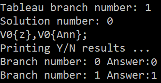
Let ψQ=⟨z,xE​v​a⟩∈XM​o​t​h​e​r3\psi_{Q}=\langle z,x_{Eva}\rangle\in X^{3}_{Mother} be a query represented in set-theoretic terms. A complete KEγ-tableau for ϕ\mathcal​K​B\phi_{\mathcal{KB}} and the decision trees constructed for the evaluation of ψQ\psi_{Q} on each open branch of the KEγ-tableau are shown in Figure 6. Notice that, the decision tree constructed on the leftmost open branch of the KEγ-tableau provides no solution.

Refer to caption
Figure 6: KEγ-tableau for ϕ\mathcal​K​B\phi_{\mathcal{KB}} and decision trees for the evaluation of ψQ\psi_{Q}.

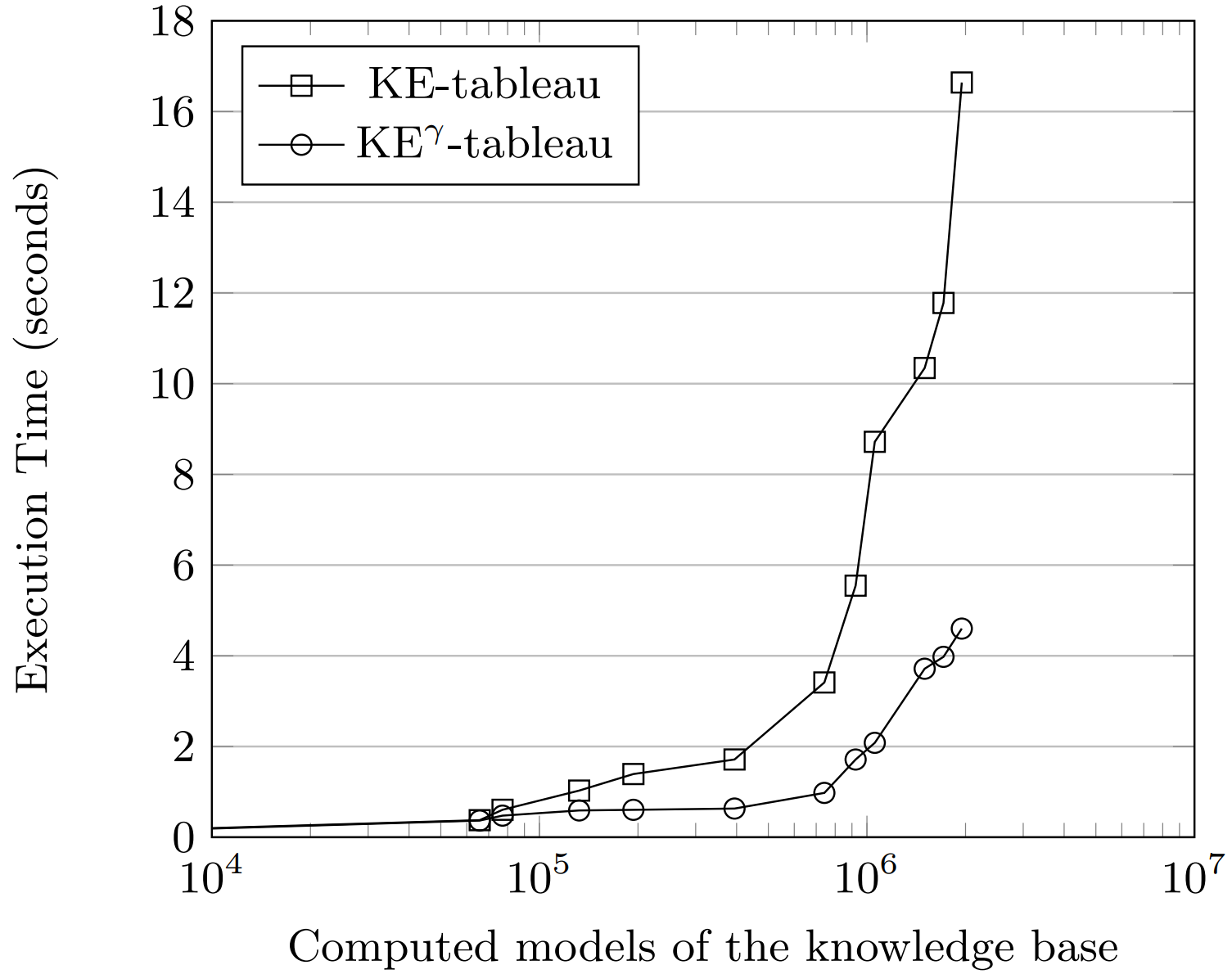
The internal representation of the OWL ontology is shown in Figure 7. The KEγ-tableau computed by the reasoner and the evaluation of the query ψQ\psi_{Q} are reported in Figure 8. Finally, Figure 9 shows a performance comparison between our implementation of the KE-tableau presented in [7] and the KEγ-tableau system for \mathcal​D​L𝐃4,×\mathcal{DL}_{\mathbf{D}}^{4,\!\times} presented in this paper. The metric used in the benchmarking is the number of models of the input KB computed by the reasoners and the time required to compute such models. As shown in Figure 9, the KEγ-tableau has a better performance than the KE-tableau up to about 400%400\%, even if in some cases the performances of the two systems are comparable, as shown in the plot. We conclude that the KEγ-tableau system is always convenient, also because the expansions of quantified formulae are not stored in memory.

Refer to caption
Figure 7: Internal representation of the ontology.
Refer to caption
Refer to caption
Figure 8: The KEγ-tableau and the evaluation of ψQ\psi_{Q} computed by the reasoner.
Refer to caption
Figure 9: Comparison between KE-tableau and KEγ-tableau systems.

4 Conclusions

We presented a C++ implementation of a KEγ-tableau system for the most widespread reasoning tasks of \mathcal​D​L𝐃4,×\mathcal{DL}_{\mathbf{D}}^{4,\!\times}, such as consistency checking of \mathcal​D​L𝐃4,×\mathcal{DL}_{\mathbf{D}}^{4,\!\times}-KBs and a generalization of the CQA problem for \mathcal​D​L𝐃4,×\mathcal{DL}_{\mathbf{D}}^{4,\!\times}, , called HOCQA problem, admitting conjunctive queries with variables of three sorts. These problems have been addressed by translating \mathcal​D​L𝐃4,×\mathcal{DL}_{\mathbf{D}}^{4,\!\times}-KBs and higher-order \mathcal​D​L𝐃4,×\mathcal{DL}_{\mathbf{D}}^{4,\!\times}-conjunctive queries in terms of formulae of the set-theoretic fragment 𝟦​𝖫​𝖰​𝖲\mathcal​D​LD4,​×𝖱\mathsf{4LQS}_{\scriptscriptstyle{\mathcal{DL}_{\lx@scalerel@obj{\mathbf{D}}}^{\lx@scalerel@obj{4,\!\times}}}}^{\mathsf{R}}. The reasoner is an improvement of the KE-tableau system introduced in [7] to check consistency of \mathcal​D​L𝐃4,×\mathcal{DL}_{\mathbf{D}}^{4,\!\times}-KBs, as it admits a generalization of the KE-elimination rule incorporating the γ\gamma-rule. The reasoner takes as input OWL ontologies compatible with the specifications of \mathcal​D​L𝐃4,×\mathcal{DL}_{\mathbf{D}}^{4,\!\times} serialized in the OWL/XML format and admitting SWRL rules.

Finally, we showed that the reasoner presented in this paper is more efficient than the one introduced in [7], by means of suitable benchmark test sets.

We plan to extend the set-theoretic fragment underpinning the reasoner to include also a restricted version of the operator of relational composition. This will allow ones to reason with description logics that admit full existential and universal quantification. In addition, we intend to improve our reasoner so as to deal with the reasoning problem of ontology classification. Then, we shall compare the resulting reasoner with existing well-known reasoners such as HermiT [11] and Pellet [17], providing some benchmarking. We also plan to allow data type reasoning by either integrating existing solvers for the Satisfiability Modulo Theories (SMT) problem or by designing ad-hoc new solvers. Finally, as each branch of the KEγ-tableau can be computed by a single processing unit, we plan to implement a parallel version of the software by using the Nvidia CUDA library.

References

  • [1] C. Cantale, D. Cantone, M. Nicolosi-Asmundo, and D.F. Santamaria. Distant Reading Through Ontologies: The Case Study of Catania’s Benedictines Monastery. JIS.it, 8,3 (September 2017).
  • [2] D. Cantone, A. Ferro, and E. G. Omodeo. Computable set theory. Number 6 in International Series of Monographs on Computer Science, Oxford Science Publications. Clarendon Press, Oxford, UK, 1989.
  • [3] D. Cantone and M. Nicolosi-Asmundo. On the satisfiability problem for a 4-level quantified syllogistic and some applications to modal logic. Fundamenta Informaticae, 124(4):427–448, 2013.
  • [4] D. Cantone, M. Nicolosi-Asmundo, and D. F. Santamaria. Conjunctive query answering via a fragment of set theory. In Proc. of ICTCS 2016, Lecce, September 7-9, CEUR-WS Vol. 1720, pp. 23–35.
  • [5] D. Cantone, M. Nicolosi-Asmundo, and D. F. Santamaria. A set-theoretic approach to ABox reasoning services. In Costantini S., Franconi E., Van Woensel W., Kontchakov R., Sadri F., Roman D. Rules and Reasoning. RuleML+RR 2017., Lecture Notes in Computer Science, vol 10364. Springer, 2017.
  • [6] D. Cantone, M. Nicolosi-Asmundo, and D. F. Santamaria. A set-theoretic approach to ABox reasoning services. CoRR, 1702.03096, 2017. Extended version.
  • [7] D. Cantone, M. Nicolosi-Asmundo, and D. F. Santamaria. A C++ reasoner for the description logic \mathcal​D​L𝐃4,×\mathcal{DL}_{\mathbf{D}}^{4,\!\times}. In Proc.of CILC 2017, 26-29 September 2017, Naples, Italy. CEUR WS, ISSN 1613-0073, Vol. 1949, pp. 276-280., 2017.
  • [8] D. Cantone, M. Nicolosi-Asmundo, and D. F. Santamaria. An optimized KE-tableau-based system for reasoning in the description logic \mathcal​D​L𝐃4,×\mathcal{DL}_{\mathbf{D}}^{4,\!\times}. CoRR, 1804.11222, 2018. Extended version.
  • [9] D. Cantone, M. Nicolosi-Asmundo, D. F. Santamaria, and F. Trapani. Ontoceramic: an OWL ontology for ceramics classification. In Proc. of CILC 2015, CEUR-WS, vol. 1459, pp. 122–127, Genova, July 1-3, 2015.
  • [10] D. Cantone, E. Omodeo, and A. Policriti. Set theory for computing: from decision procedures to declarative programming with sets. Monographs in Computer Science. Springer-Verlag, New York, NY, USA, 2001.
  • [11] B. Glimm, I. Horrocks, B. Motik, G. Stoilos, and Z. Wang. HermiT: An OWL 2 Reasoner. Journal of Automated Reasoning, 53(3):245–269, 2014.
  • [12] I. Horrocks, O. Kutz, and U. Sattler. The even more irresistible SROIQ. In Proc. 10th Int. Conf. on Princ. of Knowledge Representation and Reasoning, (Doherty, P. and Mylopoulos, J. and Welty, C. A., eds.), pages 57–67. AAAI Press, 2006.
  • [13] M. Mondadori M. D’Agostino. The taming of the cut. Classical refutations with analytic cut. Journal of Logic and Computation, 4:285–319, 1994.
  • [14] B. Motik and I. Horrocks. OWL datatypes: Design and implementation. In Proc. of the 7th Int. Semantic Web Conference (ISWC 2008), volume 5318 of LNCS, pages 307–322. Springer, October 26–30 2008.
  • [15] D. F. Santamaria. A Set-Theoretical Representation for OWL 2 Profiles. LAP Lambert Academic Publishing, ISBN 978-3-659-68797-6, 2015.
  • [16] Jacob T. Schwartz, Domenico Cantone, and Eugenio G. Omodeo. Computational Logic and Set Theory: Applying Formalized Logic to Analysis. Texts in Computer Science. Springer-Verlag New York, Inc., 2011.
  • [17] E. Sirin, B. Parsia, B. C. Grau, A. Kalyanpur, and Y. Katz. Pellet: A practical OWL-DL reasoner. J. Web Sem., 5(2):51–53, 2007.
  • [18] R. M. Smullyan. First-order Logic. Dover books on advanced Math. Dover, 1995.