Non-equilibrium correlations in minimal dynamical models of polymer copying

We consider a copy polymer ${M}=M_{1},...,M_{l}$, made up of a series of sub-units or monomers $M_{x}$, growing with respect to a template ${N}=N_{1},...,N_{L}$ ($l\leq L$). Inspired by transcription and translation, we consider a copy that detaches from the template as it grows; fig. 1b shows the simplest model of this type. We consider whole steps in which a single monomer is added or removed, encompassing many individual chemical sub-steps [2, 1]. After each step there is only a single inter-polymer bond at position $l$, between $M_{l}$ and $N_{l}$. As a new monomer joins the copy at position $l+1$, the bond position $l$ is broken, contrasting with previous models of TSA [3, 1, 4, 5, 2, 6] (Fig. 1a). Importantly, as explained below, each step now depends on both of the two leading monomers, generating extra correlations within the copy sequence.

Following earlier work, we assume that both polymers are copolymers, and that the two monomer types are symmetric [3, 1, 4, 5, 2, 6]. Thus the relevant question is whether monomers $M_{l}$ and $N_{l}$ match; we therefore ignore the specific sequence of $N$ and describe $M_{l}$ simply as right or wrong. Thus $M_{l}\in r,w$; with example chain $M=rrwwrrrrrwrr$. An excess of $r$ indicates a correlation between template and copy sequences. Breaking this symmetry would favour specific template sequences over others, disfavouring the accurate copying of other templates and compromising the generality of the process.

Given the model’s state space, we now consider state free energies (which must be time-invariant for autonomy). We treat the environment as a bath of monomers at constant chemical potential [3, 1, 4, 5, 2, 6]. By symmetry, extending the polymer while leaving the copy-template interaction unchanged involves a fixed polymerization free energy. We thus define $-\Delta G_{\rm{pol}}$ as the chemical free-energy change for the transition between any specific sequence $m_{1},...,m_{l}$ and any specific sequence $m_{1},...,m_{l+1}$, ignoring any contribution from interactions with the template. We then define $\Delta G_{\rm{TT}}$ as the effect of the free-energy difference between $r$ and $w$ interactions with template. This bias can be describes as ”temporary thermodynamic” (TT) since it only lasts until that contact is broken.

Overall, each forward step makes and breaks one copy-template bond. There are four possibilities: either adding $r$ or $w$ at position $l+1$ to a template with $M_{l}=r$; or adding $r$ or $w$ in position $l+1$ to a template with $M_{l}=w$. The first and last of these options make and break the same kind of template bond, so the total free-energy change is $-\Delta G_{\rm{pol}}$. For the second case there is a $r$ bond broken and a $w$ bond added, implying a free-energy change of $-\Delta G_{\rm{pol}}+\Delta G_{\rm{TT}}$. Conversely, for the third case, there is a $w$ bond broken and a $r$ bond added, giving a free-energy change of $-\Delta G_{\rm{pol}}-\Delta G_{\rm{TT}}$. These constraints are shown in fig. 1b; the contribution of this work is to study the consequences of these constraints. Models of TSA (fig. 1a) of equivalent complexity can be constructed, but they are not bound by these constraints and hence the underlying results and biophysical interpretation are distinct.

Having specified model thermodynamics, we now parameterize kinetics. We assume that there are no “futile cycles”, such as appear in kinetic proofreading [24]. Reactions are thus tightly coupled: each step requires a well defined input of free energy determined by $-\Delta G_{\rm{pol}}$ and $\pm\Delta G_{\rm{TT}}$ [26], and no free-energy release occurs without a step.

A full kinetic treatment would be a continuous time Markov process incorporating the intermediate states shown schematically in fig. 1b. To identify sequence output, however, we need only consider the state space in fig. 1b and the relative probabilities for transitions between these explicitly modelled states, ignoring the complexity of non-exponential transition waiting times [1]. We define propensities $\psi^{+}_{xy}$ as the rate per unit time in which a system in state $\&x$ starts the process of becoming $\&xy$ and $\psi^{-}_{xy}$ as the equivalent quantity in the reverse direction ($\&$ is an unspecified polymer sequence). Our system has eight of these propensities ($\psi^{\pm}_{rr}$, $\psi^{\pm}_{rw}$, $\psi^{\pm}_{wr}$ and $\psi^{\pm}_{ww}$); the simplest TSA models require four [3, 5, 2, 6, 1].

Prior literature on TSA [5] has differentiated between purely “kinetic” discrimination, in which $r$ and $w$ have an equal template-binding free energy but different binding rates; and purely thermodynamic discrimination in which $r$ and $w$ bind at the same rate, but $r$ is stabilized in equilibrium by stronger binding interactions. Eventually, all discrimination is “kinetic” for persistent copying, since there is no lasting equilibrium bias (Fig. 1 (b)). However, by analogy with TSA, we do consider two distinct mechanisms for discrimination - a kinetic one, in which $r$ is added faster than $w$ to the growing tip, and one based on the temporary thermodynamic bias towards correct matches at the tip of the growing polymer due to short-lived favourable interactions with the template, quantified by $\Delta G_{\rm{TT}}>0$ (Fig. 1b). The kinetic mechanism should not be conflated with fuel consuming “kinetic proofreading” cycles that can also enhance accuracy, which are not considered.

We parameterize the propensities as follows. Assuming, for simplicity, that the propensity for adding $r$ or $w$ is independent of the previous monomer, we have: $\psi^{+}_{rr}=\psi^{+}_{wr}$ and $\psi^{+}_{rw}=\psi^{+}_{ww}=1$, also defining the overall timescale. “Kinetic” discrimination is then quantified by $\psi^{+}_{xr}/\psi^{+}_{xw}=\exp(\Delta G_{\rm{K}}/k_{B}T)$. Forwards propensities are thus differentiated solely by $\Delta G_{\rm{K}}$; backwards propensities are set by fixing the ratios $\psi^{+}_{xy}/\psi^{-}_{xy}$ according to the free energy change of the reaction, which follow from $\Delta G_{\rm pol}$ and $\Delta G_{\rm TT}$ (Fig. 1(b)). Thus, setting $k_{B}T=1$,

For a given $\Delta G_{\rm{K}}$, $\Delta G_{\rm{\rm{pol}}}$ and $\Delta G_{\rm{\rm{TT}}}$, eqs. 1-4 describe a set of models with distinct intermediate states that yield the same copy sequence distribution. We can thus analyze the simplest model in each set, which is Markovian at the level of the explicitly modelled states with $\psi^{\pm}_{xy}$ as rate constants.

We use Gaspard’s method to solve the system [23]; the underlying equations can also be mapped to models of distinct physical systems that have different constraints on the parameters [Whitelam]. In this approach, the tip-monomer identity probabilities $\left(\mu(m_{l})\right)$, the joint tip and penultimate monomer identity probabilities $\left(\mu(m_{l-1},m_{l})\right)$, and the conditional probabilities $\left(\mu(m_{l-1}|m_{l})\right)$ become stationary for a long polymer and can be calculated. One must first calculate the partial velocities, $v_{r}$ and $v_{w}$. The quantity $v_{x}\mu(x)$ is the net rate at which monomers are added after an $x$,

Following ref. [23], these velocities can be solved in terms of the propensities. In turn, the velocities and propensities determine tip and conditional probabilities $\mu(m_{l})$ and $\mu(m_{l-1}|m_{l})$ [23]. Further details are provided in SI Appendix.

Gaspard’s method describes the chain while it is still growing through the stochastic variables $M_{l}$ and $M_{l-1}$, with the index $l$ being the current length of the polymer. We, however, are interested in the identity of the monomer at position $n$ when $l\gg n$. We label this ”final” state of the monomer at position $n$ as $M_{n}^{\infty}$. As discussed in the SI Index, $M_{n}^{\infty}$ is distinct from $M_{n}$ near the tip. $M_{n}^{\infty}$ is described by the error probability $\epsilon$ and the conditional error probabilities $\epsilon_{r}$ and $\epsilon_{w}$, defined as the probability that $M^{\infty}_{n+1}=w$ given that $M^{\infty}_{n}=r$ or $M^{\infty}_{n}=w$, respectively. We show that $\epsilon$, $\epsilon_{r}$ and $\epsilon_{w}$ are sufficient in the SI Appendix, by proving that the $M^{\infty}$ is a Markov chain of $r$ and $w$ monomers (this requirement is distinct from the Markovian growth dynamics). We note that $\epsilon\neq\epsilon_{r}\neq\epsilon_{w}$ as a direct result of the dependence of the transition propensities on the current and previous tip monomers, which in turn arises from detachment.

To calculate $\epsilon$, $\epsilon_{r}$ and $\epsilon_{w}$, we define currents $J_{xy}$ that are related to both $\psi^{\pm}_{xy}$ and $\epsilon$, $\epsilon_{r}$ and $\epsilon_{w}$ separately. The current $J_{xy}$ is the net rate per unit time at which transitions $\&x\rightarrow\&xy$ occur: $J_{xy}=\psi_{xy}^{+}\mu(x)-\psi_{xy}^{-}\mu(x,y)$. By considering the transitions in our system as a tree, as in Fig. 2, we can relate the current through a branch to the overall rate at which errors are permanently incorporated into a polymer growing at total velocity $v=v_{r}\mu(r)+v_{w}\mu(w)$

Eliminating $\epsilon$ from the simultaneous equations 6-9 yields $\epsilon_{r}$ and $\epsilon_{w}$ in terms of known quantities. To find $\epsilon$, note that the final sequence has a transition matrix parameterized by $\epsilon_{r}$ and $\epsilon_{w}$, with the overall error $\epsilon$ given by its dominant eigenvector. As detailed in the SI Appendix, we obtain $\epsilon={\epsilon_{r}}/{(1+\epsilon_{r}-\epsilon_{w})}$. From $\epsilon$, $\epsilon_{r}$ and $\epsilon_{w}$ we calculate properties of the copy in terms of $\psi^{\pm}_{xy}$ and thus the free energies. We corroborate the analytical results with simulation (see SI Index).

The free energy of the combined bath and polymer system decreases over time. There are two contributions to the free-energy change per added monomer: the chemical free energy $\Delta G_{\rm{pol}}$, and a contribution from the uncertainty of the final polymer sequence [7]. The latter is quantified by the entropy rate $H$ [27, 28]:

which in our case is given by [28]

The overall free energy change per added monomer is then $\Delta G_{\rm{tot}}=-\Delta G_{\rm{pol}}-H$, which must be negative for growth: $H\geq-\Delta G_{\rm pol}$. Since copy-template interactions are not extensive in the copy length, they do not contribute. Given that $H\geq 0$, growth is possible in the region where $\Delta G_{\rm{pol}}<0$, corresponding to the “entropically driven” regime [6, 3].

The entropy rate is bounded by the single site entropy $H\leq H_{ss}=-\epsilon\ln{\epsilon}-(1-\epsilon)\ln{(1-\epsilon)}$. $H_{ss}$ quantifies the desired correlations between copy and template. For previous models of TSA with uncorrelated monomer incorporation, $H=H_{ss}$ [3, 1, 4, 5, 2, 23, 6]. In our model, the necessary complexity of $\psi^{\pm}_{xy}$ generates correlations within the copy. A stronger constraint on the single site entropy, and hence accuracy, then follows: $H_{ss}\geq H\geq-\Delta G_{\rm{\rm{pol}}}$.

Fundamentally, a persistent copy is a high free energy state, as the entropic cost of copy-template correlations cannot be counteracted by stabilizing copy-template interactions. Thus the process moves a system between two high free energy states, converting chemical work into correlations. In general, only a fraction of the chemical work done by the monomer bath is retained in the final state, implying dissipation, and so it is natural to introduce an efficiency. The overall free energy stored in the polymer has contributions both from the creation of an equilibrium (uncorrelated) polymer and from correlations within the copy and with the template. We are interested only in the contributions above equilibrium. The efficiency $\eta$ is then the proportion of the additional free energy expended in making a copy above the minimum required to grow a random equilibrium polymer that is successfully converted into the non-equilibrium free energy of the copy sequence rather than being dissipated. In our simple case,

Here, $\Delta G_{\rm{pol}}+H_{\rm eq}=\Delta G_{\rm{pol}}+\ln 2$ is the extra chemical work done by the buffer above that required to grow an equilibrium polymer, $\Delta G_{\rm pol}^{\rm eq}=-H_{\rm eq}=-\ln 2$. The free energy stored in the copy sequence, above that stored in an equilibrium system, is $H_{\rm eq}-H$. $\eta\leq 1$ follows from $\Delta G_{\rm{pol}}+H\geq 0$. Similarly, since $H_{\rm ss}\geq H$ we can define a single-site efficiency

Unlike $\eta$, the single site efficiency $\eta_{\rm ss}$ discounts the free energy stored in “useless” correlations within the copy.

We consider three representative models consistent with eqs. 1-4. First, the purely kinetic mechanism obtained by setting $\Delta G_{\rm{TT}}=0$ and $\Delta G_{\rm{K}}=\Delta G$ in equations 1-4. Originally proposed by Bennett for TSA [3], it is coincidentally a limiting case of persistent copying since there is no equilibrium bias. We also consider two new mechanisms: pure “temporary thermodynamic discrimination” with $\Delta G_{\rm{K}}=0$ and $\Delta G_{\rm{TT}}=\Delta G$, and a “combined discrimination mechanism”, in which both template binding strengths and rates of addition favour $r$ monomers: $\Delta G_{\rm{K}}=\Delta G_{\rm{TT}}=\Delta G$.

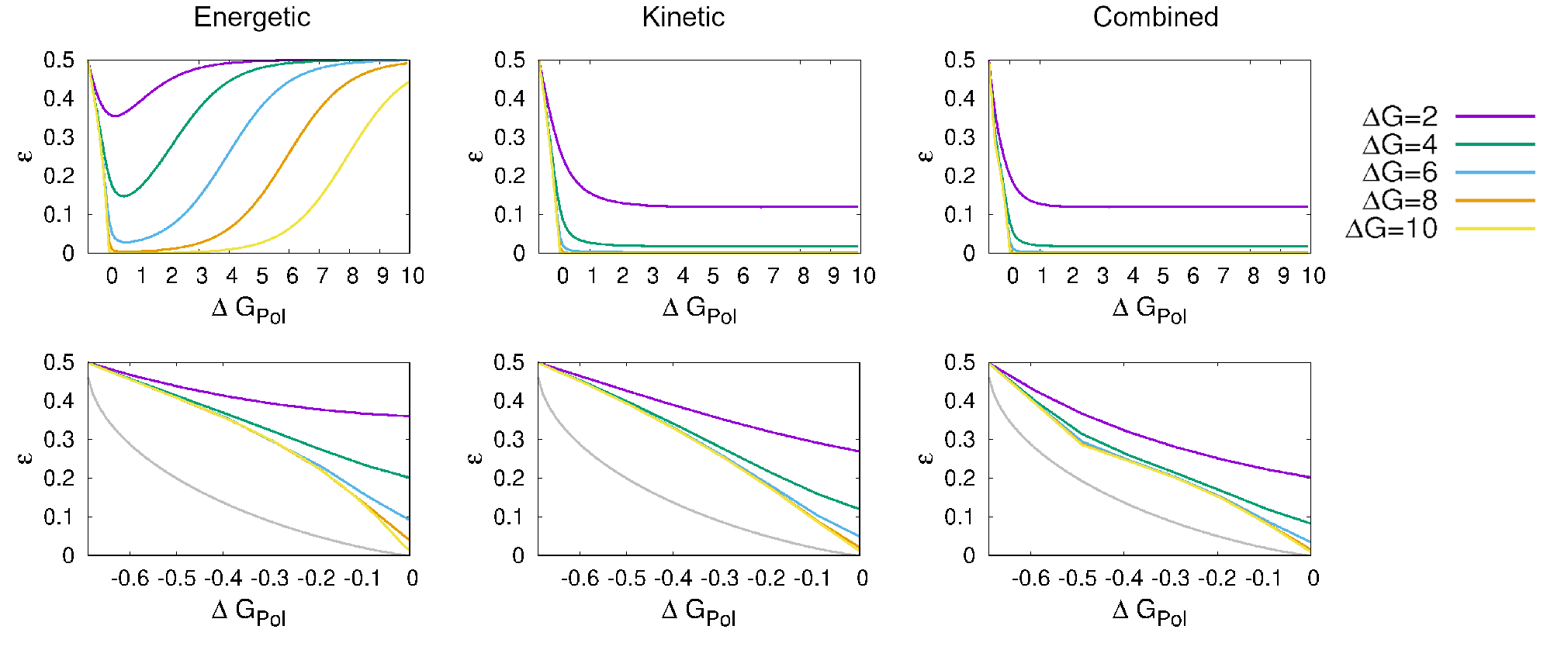
All three mechanisms have two free parameters, the overall driving strength $\Delta G_{\rm{pol}}$ and the discrimination parameter $\Delta G$. We plot error probability against $\Delta G_{\rm{pol}}$ for various $\Delta G$ in fig. 3. Also shown is the thermodynamic lower bound on $\epsilon$ implied by $H_{\rm ss}\geq H\geq-\Delta G_{\rm{\rm{pol}}}$. All three cases have no accuracy ($\epsilon=0.5$) in equilibrium ($\Delta G_{\rm pol}\rightarrow-\ln 2$) since an accurate persistent copy is necessarily out of equilibrium [7]. By contrast, TSA allows for accuracy in equilibrium [5, 2, 29].

The temporary thermodynamic mechanism is always the least effective. It has no accuracy for high $\Delta G_{\rm pol}$ as the difference between $r$ and $w$ is only manifest when stepping backwards, and for high $\Delta G_{\rm pol}$ back steps are rare [5, 2]. More interestingly, temporary thermodynamic discrimination is also inaccurate as $\Delta G_{\rm pol}\rightarrow-\ln 2$, when the system takes so many back steps that it fully equilibrates. Low $\epsilon$ only occurs when $\Delta G_{\rm{pol}}$ is sufficient to inhibit the detachment of $r$ monomers, but not the detachment of $w$ monomers. This trade-off region grows with $\Delta G$. By contrast, both the combined case and the kinetic case have accuracy in the limit of $\Delta G_{\rm{pol}}\rightarrow\infty$, since they allow $r$ to bind faster than $w$. Considering $\Delta G_{\rm pol}\leq 0$ closely (fig. 3b) shows the combined case to be superior.

Intriguingly, all three mechanisms are far from the fundamental bound on $\epsilon$ implied by $H_{\rm ss}\geq H\geq-\Delta G_{{\rm{pol}}}$ as $\Delta G_{\rm{pol}}\rightarrow-\ln{2}$, and there is an apparent cusp in $\epsilon$ at $\Delta G_{\rm pol}\approx 0.48$ as $\Delta G\rightarrow\infty$ in the combined case. The performance relative to the bound is quantified by $\eta_{\rm ss}$ (fig. 4). Surprisingly, we observe in fig. 4a that not only does $\epsilon$ go to zero as $\Delta G_{\rm pol}\rightarrow-\ln 2$, so does $\eta_{ss}$ in all cases. For small non-equilibrium driving, none of the extra chemical work input is stored in correlations with the template. Mathematically, this inefficiency arises because $\epsilon-0.5\propto\Delta G_{\rm{pol}}-\ln{2}$ as $\Delta G_{\rm pol}\rightarrow-\ln 2$ (as observed in fig. 3), and $H_{\rm ss}-\ln 2\propto(\epsilon-0.5)^{2}$ for $\epsilon\approx 0.5$ by definition. Thus, from equation 13, $\eta_{\rm ss}\propto\Delta G_{\rm{pol}}-\ln{2}$ as $\Delta G_{\rm pol}\rightarrow-\ln 2$. That this result only depends on error probability decreasing proportionally with $\Delta G_{\rm{pol}}$ for small driving suggests that a vanishing $\eta_{ss}$ in equilibrium may be quite general.

In all cases, the single-site efficiency $\eta_{\rm ss}$ increases from 0 at $\Delta G_{\rm pol}=-\ln 2$ to a peak near $\Delta G_{\rm pol}=0$, with $\eta_{\rm ss}\rightarrow 1$ as $\Delta G\rightarrow\infty$. Beyond this peak, $\eta_{\rm ss}$ drops as the stored free energy is bounded by $\ln{2}$ per monomer. To understand the peak, note that for every $\Delta G_{\rm{pol}}\leq 0$ there is a hypothetical highest accuracy copy with $\epsilon$ fixed by $H_{\rm ss}=-\Delta G_{\rm{pol}}$ that is marginally thermodynamically permitted. However, this copy is not usually kinetically accessible. At $\Delta G_{\rm{pol}}=0$ the marginal copy has 100% accuracy and, unusually, all three mechanisms can approach it kinetically, causing a peak. The efficiency approaches its limit of unity even for moderate values of $\Delta G$. We note that as $\Delta G\rightarrow\infty$, growth is slow for $\Delta G_{\rm pol}\leq 0$: the total number of steps taken diverges.

A related argument explains the apparent cusp in the error $\epsilon$ for the combined mechanism at $\Delta G_{\rm{pol}}\approx-0.48$ and high $\Delta G$. On the plot of $\eta_{\rm ss}$ (fig. 4 a) this cusp manifests as a shoulder. The full efficiency $\eta$ (fig. 4 b) has a prominent second peak. Uniquely, the combined mechanism’s kinetics strongly disfavour chains of consecutive $w$s for high $\Delta G$. A final copy with no consecutive $w$s has $\epsilon_{w}=0$ but $\epsilon_{r}\neq 0$. Maximizing the entropy rate of such a Markov chain over $\epsilon_{r}$ gives $H_{\rm max}=0.48121$; $\Delta G_{\rm pol}=-H_{\rm max}$ matches the location of our peak/cusp. Thus the combined mechanism initially eliminates consecutive $w$s, and at $\Delta G_{\rm pol}=-0.48121$ a state with $\eta_{w}=0$ is thermodynamically permitted for the first time. For large $\Delta G$, this polymer is kinetically accessible and grows with thermodynamic efficiency approaching unity (fig. 4 c). In this limit, the overall entropy generation is zero.

The above behaviour is a striking example of correlations being generated within the copy sequence, as well as with the template. Notably, whilst $\eta$ approaches unity at this point, $\eta_{\rm ss}$ does not (fig. 4). Correlations within the copy sequence limit the chemical work that can be devoted to improving the single site accuracy of the copy polymer, since they prevent the bound $H_{\rm ss}\geq H\geq-\Delta G_{{\rm{pol}}}$ from being saturated.

Following ref. [23], the partial velocities can also be expressed as

for $x=r,w$. This gives a pair of simultaneous equations that can be solved for the partial velocities in terms of the propensities. In turn, the velocities and propensities determine tip and conditional probabilities $\mu(m_{l})$ and $\mu(m_{l-1}|m_{l})$, with $m_{l},m_{l-1}\in\{r,w\}$, via

It might not be immediately obvious why the properties of the growing chain described by $\mu(m_{l})$ and $\mu(m_{l},m_{l-1})$ should be different from those of the final chain described by $\epsilon$, $\epsilon_{r}$ and $\epsilon_{w}$, but the difference can be illustrated with a simple example. Consider a system in which incorrect monomers could be added to the end of the chain, but where nothing can be added after an incorrect match. In this case while the tip probability for an incorrect match $\mu(w)$ would be finite, the error of the final chain $\epsilon$ would be vanishingly small, as all incorrect matches would have to be removed in order for the polymer to grow further.

Let $M^{\infty}_{n}$ be the monomer at the $n$th site in the final chain. Let a polymer be represented by $M^{\infty}_{1},...,M^{\infty}_{n}$. The probability of a given chain existing is then $P^{\infty}(m_{1},...,m_{n})$. In order for the sequence of monomers moving along the chain (increasing $n$) to be able to be represented by a Markov chain, the condition

must hold.

In order to demonstrate that eq. 17 holds, we rewrite the final chain probability in terms of properties of the growing chain. Specifically we state that the probability of the sequence $m_{1},...,m_{n}$ existing in the final chain is the product of the probability $Q(m_{1},...,m_{n-1},t)$ that the chain is in the state $m_{1},...,m_{n-1}$ at a time $t$ during the growth process, and the propensity $\nu(m_{n};m_{1},...,m_{n-1})$ with which $m_{n}$ is added to a chain $m_{1},...,m_{n-1}$ and never removed, integrated over all time. It should be noted that $r(m_{n};m_{1},...,m_{n-1})$ is time-independent.

Setting the integral equal to $I(m_{1},...,m_{n-1})$ gives

Let’s consider the probabilities of two sub-sequences, identical except for the final monomer. We call the two final monomers $m_{n}$ and $m^{\prime}_{n}$ and we can denote the ratios of the probabilities of these two chains as follows.

The $I$ terms are independent of this final monomer and so cancel. Thus

The same relationship holds for the conditional probabilities

For our system, the propensity with which a monomer $m_{n}$ is added and never removed, $\nu(m_{n};m_{1},...,m_{n-1})$, is dependent on only on the final two monomers in the sequence fragment, $m_{n}$ and $m_{n-1}$. To see why, note that this propensity is determined by addition and removal of monomers at sites $i\geq n$. The identities of monomers at positions $j<n-1$, however, only influence addition and removal propensities at sites $k<n$ (eq. 1-4 main text). Thus we convert $\nu(m_{n};m_{1},...,m_{n-1})$ to $f(m_{n},m_{n-1})$.

Multiplying both sides by $P^{\infty}(m_{1},...,m_{n-2})$ and summing over all values of $m_{1},...m_{n-2}$ (recall $\sum_{c,d}P(a|b,c,d)P(c,d)=P(a|b)$ and $\sum_{c,d}P(c,d)=1$) gives

Comparing equations 24 and 25 yields:

Summing over the possible values of $m^{\prime}_{n}$ and recalling that $P^{\infty}(r|m_{n-1})+P^{\infty}(w|m_{n-1})=1$ and $P^{\infty}(r|m_{n-1},...,m_{1})+P^{\infty}(w|m_{n-1},...,m_{1})=1$ yields:

thereby proving that the sequence of the final chain is Markovian.

The final sequence is described by the Markov chain illustrated in figure 5. The transition matrix for this process is

The eigenvector of this transition matrix with eigenvalue equal to unity gives the steady state of the Markov chain. The second component of this eigenvector corresponds to the overall probability of incorrect matches, $\epsilon$:

To check the analytical methods used to solve the system we also simulated the growth of a polymer. We used a Gillespie simulation [32], with transition rates given by $\psi^{\pm}_{xy}$. Simulations were initialised with a randomly determined two monomer sequence, and truncated as soon as the polymer reached 1000 monomers. We found that such a length rendered edge effects negligible in all but the most extreme cases for the calculation of $\epsilon$. Polymer error probabilities were inferred directly from the 100 simulations, and are compared to analytical results in fig. 6.

We note in passing that the calculation of $H$, $H_{ss}$, and particularly the efficiency’s $\eta$ and $\eta_{ss}$, are more vulnerable to random fluctuations in a simulation of finite length, and peculiar edge effects, than $\epsilon$. Gaspard’s solution is therefore invaluable in reaching robust conclusions for these quantities.

References

- [1] Cady F, Qian H (2009) Open-system thermodynamic analysis of DNA polymerase fidelity. PHYS BIOL 6:036011.
- [2] Sartori P, Pigolotti S (2015) Thermodynamics of error correction. PHYS REV X 5:041039.
- [3] Bennett CH (1979) Dissipation-error tradeoff in proofreading. BIOSYSTEMS 11:85–91.
- [4] Andrieux D, Gaspard P (2008) Nonequilibrium generation of information in copolymerization processes. PROC NAT ACAD SCI USA 105:9516–9521.
- [5] Sartori P, Pigolotti S (2013) Kinetic versus energetic discrimination in biological copying. PHYS REV LETT 110:188101.
- [6] Esposito M, Lindenberg K, Van den Broeck C (2010) Extracting chemical energy by growing disorder: efficiency at maximum power. J STAT MECH-THEORY E 2010:P01008.
- [7] Ouldridge TE, ten Wolde PR (2017) Fundamental costs in the production and destruction of persistent polymer copies. PHYS REV LETT 118:158103.
- [8] Ouldridge TE, Govern CC, ten Wolde PR (2017) Thermodynamics of computational copying in biochemical systems. Phys. Rev. X 7:021004.
- [9] Tjivikua T, Ballester P, Rebek Jr J (1990) Self-replicating system. J AMM PHYS SOC 112:1249–1250.
- [10] Feng Q, Park TK, Rebek J (1992) Crossover reactions between synthetic replicators yield active and inactive recombinants. SCIENCE 256:1179–1180.
- [11] Vidonne A, Philp D (2009) Making molecules make themselves–the chemistry of artificial replicators. EUR J ORG CHEM 2009:593–610.
- [12] Orgel LE (1992) Molecular replication. NATURE 358:203.
- [13] Colomb-Delsuc M, Mattia E, Sadownik JW, Otto S (2015) Exponential self-replication enabled through a fibre elongation/breakage mechanism. NAT COMMUN 6:7427.
- [14] Sievers D, Von Kiedrowski G (1994) Self-replication of complementary nucleotide-based oligomers. NATURE 369:221–224.
- [15] Lincoln TA, Joyce GF (2009) Self-sustained replication of an RNA enzyme. SCIENCE 323:1229–1232.
- [16] Wu N, Willner I (2016) ph-stimulated reconfiguration and structural isomerization of origami dimer and trimer systems. NANO LETT 16:6650–6655.
- [17] Wang T, et al. (2011) Self-replication of information-bearing nanoscale patterns. NATURE 478:225–228.
- [18] Li T, Nicolaou K (1994) Chemical self-replication of palindromic duplex dna. NATURE 369:218–221.
- [19] Mast CB, Braun D (2010) Thermal trap for DNA replication. PHYS REV LETT 104:188102.
- [20] Orgel LE (1998) The origin of life—a review of facts and speculations. TRENDS BIOCHEM SCI 23:491–495.
- [21] Martin W, Baross J, Kelley D, Russell MJ (2008) Hydrothermal vents and the origin of life. NAT REV MICROBIOL 6:805.
- [22] Schulman R, Yurke B, Winfree E (2012) Robust self-replication of combinatorial information via crystal growth and scission. PROC NAT ACAD SCI USA 109:6405–6410.
- [23] Gaspard P, Andrieux D (2014) Kinetics and thermodynamics of first-order markov chain copolymerization. J CHEM PHYS 141:044908.
- [24] Hopfield JJ (1974) Kinetic proofreading: A new mechanism for reducing errors in biosynthetic processes requiring high specificity. PROC NAT ACAD SCI USA 71:4135–4139.
- [25] Ninio J (1975) Kinetic amplification of enzyme discrimination. BIOCHIMIE 57:587–595.
- [26] Esposito M (2018) Thermodynamically consistent coarse graining of biocatalysts beyond michaelis–menten. B AM PHYS SOC.
- [27] Boyd AB, Mandal D, Crutchfield JP (2016) Identifying functional thermodynamics in autonomous maxwellian ratchets. NEW J PHYS 18:023049.
- [28] Cover TM, Thomas JA (2012) Elements of information theory. (John Wiley & Sons).
- [29] Johansson M, Lovmar M, Ehrenberg M (2008) Rate and accuracy of bacterial protein synthesis revisited. CURR OPIN MICROBIOL 11:141–147.
- [30] John SantaLucia J, Hicks D (2004) The thermodynamics of DNA structural motifs. Annu. Rev. Biophys. and Biomol. Struct. 33:415–440.
- [31] Ehrenberg M, Blomberg C (1980) Thermodynamic constraints on kinetic proofreading in biosynthetic pathways. BIOPHYS J 31:333 – 358.
- [32] Gillespie DT (1977) Exact stochastic simulation of coupled chemical reactions. J CHEM PHYS 81:2340–2361.
Supplementary Information
Solving for partial velocities and tip probabilities