The elastic and directed percolation backbone
Abstract
We argue that the elastic backbone (EB) (union of shortest paths) on a cylindrical system, recently studied by Sampaio Filho et al. [Phys. Rev. Lett. 120, 175701 (2018)], is in fact the backbone of two-dimensional directed percolation (DP). We simulate the EB on the same system as considered by these authors, and also study the DP backbone directly using an algorithm that allows backbones to be generated in a completely periodic manner. We find that both the EB in the bulk and the DP backbone have a fractal dimension of at the identical critical point . We also measure the fractal dimension at the edge of the EB system and for the full DP clusters, and find . We argue that those two fractal dimensions follow from the DP exponents as and . Our fractal dimensions differ from the value 1.750(3) found by Sampaio Filho et al.
pacs
64.60.ah, 64.60.De, 05.70.Jk, 05.70.+qBackbones in percolation systems play a central role in conductivity, permeability, and elasticity, and have been the subject of much research (i. e., [1, 2, 3, 4, 5]). Recently, Sampaio Filho et al. [6] have studied the elastic backbone (EB) in percolating systems. The EB was originally introduced by Herrmann et al. [7] as the shortest path or ensemble of shortest paths, all the same length, between two points. In [6], this was generalized to a cylindrical system—that is, a square with periodic boundaries in the horizontal direction and open boundaries on the top and the bottom, with the EB defined as the union of shortest paths between occupied sites on the top and occupied sites on the bottom. Here sites are occupied with probability as in ordinary percolation and path(s) from the top to the bottom are identified.
Below the ordinary percolation transition point [8, 9, 10], there are no crossing clusters in the system and therefore no paths. For , the authors of Ref. [6] find that there exists of the order of one shortest path. Above a second transition point at , they found the very interesting result that the fraction of the sites in the system that belong to the EB grows rapidly and gives rise to an apparent second-order transition. For site percolation on a square lattice rotated by 45∘, they find
In fact, the value coincides with the site directed percolation (DP) threshold, whose value is [11, 12, 13]. That this process corresponds to DP can be understood by the following simple argument: when the DP threshold is reached, it is possible to have a path that steps down occupied sites at each value of , and therefore has the minimum total length of on the lattice. But once one such backbone can be generated, other equal minimal paths can also occur. Especially, when , there will be multiple backbones, and an apparent transition will be observed.

To show that this hypothesis is valid, we study both the original EB model discussed by Simpaio et al., and directly the backbones of DP, which are shown in Fig. 1. We find consistent behavior in both of the studies and find values of fractal dimensions that appear to be new, and differ from the fractal dimension found in Ref. [6].
The elastic backbone. As in [6], we consider site percolation on an “tilted” square lattice with open and periodic boundary conditions along the vertical and horizontal directions, respectively. For this set of simulations we represent the lattice as an square of vertices, with diagonals, and the effective aspect ratio (height to circumference) is . We randomly occupy each lattice site with probability , construct the cluster from the top edge by the breadth-first search algorithm, and then “burn out” those “dangling” sites which do not belong to any shortest path connecting the top and the bottom edge. We measure the following observables as a function of site probability :
- •
the spanning probability connecting the top and bottom boundaries.
- •
the shortest-path length averaged over all realizations including non-spanning ones, where we set for .
- •
the average number of occupied EB sites at the top and bottom edges .
- •
the number of occupied EB sites along the centerline, representing the behavior in the bulk .
- •
the average number of occupied sites per row in all the rows of the EB, .
The system undergoes a standard percolation transition at where the spanning probability jumps to a value less than 1 (depending upon geometry), the number of shortest paths connecting the top and bottom edges is , and their length scales as with [5, 17].
At , Sampaio Filho et al. observed [6] that the system undergoes another transition in the dense phase, at which the number of shortest-paths starts to diverge and the total mass of the union of the shortest paths scales with a new fractal dimension . Together with other observations, the authors claim a novel universality class.
We conjecture that the transition at is precisely equivalent to site DP on the square lattice, which has the threshold at and a set of critical exponents as , , , and [11].
Here we carried out simulations for 7, 15, 31,…, 8191 and 15383. Figure 2 shows the results for and as a function of . It is observed that diverges at the ordinary site threshold and converges to a constant for . Near and above , is consistent with the value 1 within a statistical uncertainty for . In the whole region , remains constant, suggesting that the number of paths connecting the top and bottom boundaries is . For , diverges as increases. That goes to 1 implies that the backbones simply grow sequentially from to for .
Figure 3 shows plots of , and at as a function of , demonstrating that their scalings are governed by different exponents. The least-squares fitting to the ansatz (see Supplementary Material (SM)) gives , . We subtract 1 from the two-dimensional fractal dimensions because we are taking one-dimensional cuts through the clusters to find and .
We conjecture that the two fractal exponents above can be found from scaling arguments. For the full DP clusters, we expect that the fractal dimension satisfies the scaling relation
| (1) |
with which gives the correlation length in the parallel (time-like) direction. For the backbones, we have to eliminate the probability of growing finite clusters, so we subtract off the exponent corresponding to the survival probability, . This gives:
| (2) |
Indeed, our numerical results for and are in excellent agreement with the DP values above. To find the behavior accurately, we considered the local slope or equivalently the -dependent exponents as from two consecutive values of . The results, shown in in Fig. 7 in SM, clearly suggest that as increases, and converge to the theoretically predicted values.

Figure 4 shows the results for and at different , rescaled by the DP exponents and , respectively, as functions of . We find nearly perfect crossing at the point , giving strong evidence that the transition is at . By fixing and as in (1) and (2), the least-squares fitting gives and from , and and from , in excellent agreement with (and nearly as precise as) .
Directed percolation. We also studied DP directly on the cylindrical system, verifying that it has the same properties as the EB at . DP has been the object of a great deal of study over the years (i.e., [18, 19, 20, 13]), although it seems that this aspect of it—the fractal behavior of a collection of multiple clusters and backbones—has not been studied previously. Backbones of individual DP clusters have been discussed in the context of the de-pinning transition in invasion processes [21, 22]. A single backbone is not a fractal object but an affine one with a roughness exponent of . It is only when one considers the collection of DP backbones that span the system as occurs in the cylindrical system is the fractal nature manifest. Fractal properties of single DP clusters have been discussed by Kaiser and Turban [23].
To find the DP backbone, one has to trim all branches off that do not make it to the bottom of the system. Once trimmed of all downward-pointing branches, the DP backbone will be isotropic in both directions, although it still has a top and bottom edge, similar to what is seen in Fig. 1b of Ref. [6] for the EB. In Fig. 1 we show the complete clusters of DP (all sites) and the trimmed backbone (all sites except red sites).
We can further make the backbone independent of the horizontal boundaries by continuing to wrap the backbone around, in both upwards and downwards directions, removing all sites no longer connected. This procedure yields the black sites in Fig. 1, the blue and green ones being discarded. This leaves DP backbones that are periodic and having up-down symmetry. That is, if we started upwards from any row instead of downwards from the top, we would end up with the same EB for the same set of occupied sites.
We carried out simulations on systems with the above trimming procedures. Here we considered every other site of the square lattice, shifting by one each row, so we considered total sites with an aspect ratio of 1. We considered , 64,, simulating samples for the five smallest systems, and , and for the three largest systems. We measured the number of sites in the full DP clusters, , and the number of sites in the black backbone . These are plotted as a function of in Fig. 5. By examining the local slopes, we deduce (see Fig. 8) in SM and , and a more careful fitting of the data give and (see SM), which precisely agree with the predictions of equations (1) and (2).

We are not aware of any previous measurement of either of these fractal dimensions. In comparison, the backbone of ordinary percolation has a dimension of [24], and the backbone of Eden clusters has a fractal dimension is 4/3 [25]. The fractal dimension for rigidity percolation is [26, 27, 28].
Wrapping probability. Crossing and wrapping in DP behaves much differently than in ordinary percolation, where the probability to cross or wrap a system at criticality is less than 1. (For examples, the probability to cross an open square at criticality is [29, 30], to cross an open cylinder is (aspect ratio 1) or (aspect ratio 1/2) [14, 15, 16], and the probability to wrap a square torus is [31, 32].) For DP, on the other hand, we find that the probability of crossing or wrapping a cylinder jumps directly to 1 at the critical point. This is evidently because of linear behavior of the DP clusters in the large- limit, which follows from the asymmetry of the exponents and . Clusters are long and thin and thus more easily span the system.
We measured the probability that at least one DP backbone wraps around the system in the vertical direction in the fully periodic version of our problem (the black backbones in Fig. 1). We did this for at , and found values of close to 1, as given in Table 4, SM. We conjecture that behaves as
| (3) |
and find that the data are consistent with assuming , which might be expected for a system with periodic b. c. where there are no surface effects. Assuming , we can take two logarithms of (3) to write
| (4) |
A plot of the data (Fig. 6) shows good linear behavior for all and implies and .
It seems reasonable to conjecture that the exponent in (3) is proportional to the average number of wraparound backbone clusters in the system. Indeed, we measured as a function of , and plotting on a log-log plot (Fig. 6) we see that for large , , whose exponent is nearly identical to in (3). This confirms our conjecture about the behavior of being related to .
We also predict that , since the width of clusters grows as and the width of the system grows as , so . Our data for both and (large ) are consistent with this value of . We can put all these results together to write
| (5) |
where . One can interpret as the probability that a given wraparound backbone cluster does not survive.

Conclusions. The authors of Ref. [6] have uncovered that buried within supercritical percolation there exists an interesting EB transition which is related to a problem of DP. The fractal properties of the EB are exactly related to DP critical exponents, which we verify with careful simulations on both the EB and DP directly. The fractal dimension found in [6] is about halfway between the edge and bulk fractal dimensions (1) and (2), and this value evidently represents a different quantity than we are measuring here. This question deserves further investigation.
Acknowledgments. This work was partly supported by the National Science Fund for Distinguished Young Scholars (NSFDYS) under Grant No. 11625522 and the Ministry of Science and Technology of China Grant No. 2016YFA0301604 (YD). The authors thank Hans Herrmann for useful comments on the manuscript.
References
- [1] H. J. Herrmann and H. E. Stanley, Phys. Rev. Lett. 53, 1121 (1984).
- [2] T. A. Larson, J. Phys. A 20, L291 (1987).
- [3] H. Saleur, Nucl. Phys. B 382, 486 (1992).
- [4] Y. Deng, H. W. J. Blöte, and B. Nienhuis, Phys. Rev. E 69, 026114 (2004).
- [5] Z. Zhou, J. Yang, Y. Deng, and R. M. Ziff, Phys. Rev. E 86, 061101 (2012).
- [6] C. I. N. Sampaio Filho, J. S. Andrade Jr., H. J. Herrmann, and A. A. Moreira, Phys. Rev. Lett. 120, 175701 (2018).
- [7] H. J. Herrmann, D. C. Hong, and H. E. Stanley, J. Phys. A Math. Gen. 17, L261 (1984).
- [8] J. L. Jacobsen, J. Phys. A: Math. Th. 48, 454003 (2015).
- [9] Y. Yang, S. Zhou, and Y. Li, Entertainment Computing 4, 105 (2013).
- [10] X. Feng, Y. Deng, and H. W. J. Blöte, Phys. Rev. E 78, 031136 (2008).
- [11] I. Jensen, J. Phys. A. 32, 5233 (1999).
- [12] J. W. Essam, A. J. Guttmann, and K. De’Bell, J. Phys. A: Math. Gen. 21, 3815 (1988).
- [13] J. Wang, Z. Zhou, Q. Liu, T. M. Garoni, and Y. Deng, Phys. Rev. E 88, 042102 (2013).
- [14] J. Cardy, J. Stat. Phys 125, 1 (2006).
- [15] J.-P. Hovi and A. Aharony, Phys. Rev. E 53, 235 (1996).
- [16] R. M. Ziff, Phys. Rev. E 83, 020107 (2011).
- [17] P. Grassberger, J. Phys. A: Math. Gen. 25, 5475 (1992).
- [18] S. R. Broadbent and J. M. Hammersley, Math. Proc.. Cambridge Phil. Soc. 53, 629 (1957).
- [19] R. Durrett, Annals of Probability 12, 999 (1984).
- [20] G. Ódor, Rev. Mod. Phys. 76, 663 (2004).
- [21] S. V. Buldyrev, A.-L. Barabási, F. Caserta, S. Havlin, H. E. Stanley, and T. Vicsek, Phys. Rev. A 45, R8313 (1992).
- [22] L.-H. Tang and H. Leschhorn, Phys. Rev. A 45, R8309 (1992).
- [23] C. Kaiser and L. Turban, J. Phys. A: Math. Gen. 27, L579 (1994).
- [24] X. Xu, J. Wang, Z. Zhou, T. M. Garoni, and Y. Deng, Phys. Rev. E 89, 012120 (2014).
- [25] S. S. Manna and D. Dhar, Phys. Rev. E 54, R3063 (1996).
- [26] C. Moukarzel and P. M. Duxbury, Phys. Rev. Lett. 75, 4055 (1995).
- [27] D. J. Jacobs and M. F. Thorpe, Phys. Rev. Lett. 80, 5451 (1998).
- [28] C. Moukarzel and P. M. Duxbury, Phys. Rev. E 59, 2614 (1999).
- [29] J. L. Cardy, J. Phys. A: Math. Gen. 25, L201 (1992).
- [30] R. M. Ziff, Phys. Rev. Lett. 69, 2670 (1992).
- [31] H. T. Pinson, J. Stat. Phys. 75, 1167 (1994).
- [32] M. E. J. Newman and R. M. Ziff, Phys. Rev. E 64, 016706 (2001).
Supplementary Data
The elastic and directed percolation backbone
Youjin Deng and Robert M. Ziff
The Supplementary Material contains additional plots of the data, and tables of the data plotted in some of the figures.
I Additional plots


II Data
The following tables show the data given in various plots.
| 0 | 0.0004 | 0.0008 | |||
|---|---|---|---|---|---|
| 511 | 137.137(21) | 139.948(21) | 142.762(93) | 145.551(21) | 148.340(20) |
| 1023 | 240.778(63) | 248.495(63) | 255.995(21) | 263.470(61) | 270.818(60) |
| 2047 | 417.83(15) | 438.70(15) | 458.75(4) | 478.55(15) | 498.13(14) |
| 4095 | 712.20(29) | 767.54(30) | 821.81(6) | 875.09(28) | 926.26(26) |
| 8191 | 1177.52(47) | 1326.25(47) | 1472.03(11) | 1612.47(44) | 1745.23(41) |
| 0 | 0.0004 | 0.0008 | |||
|---|---|---|---|---|---|
| 511 | 66.774(16) | 68.574(16) | 70.358(7) | 72.168(16) | 74.024(16) |
| 1023 | 104.469(41) | 108.847(42) | 113.137(15) | 117.496(43) | 121.932(43) |
| 2047 | 160.972(89) | 171.378(92) | 181.626(24) | 192.316(96) | 203.004(95) |
| 4095 | 242.13(15) | 266.47(16) | 291.43(3) | 316.97(17) | 343.41(17) |
| 8191 | 351.57(21) | 408.55(22) | 467.58(6) | 529.76(24) | 593.10(25) |
| 7 | |||
|---|---|---|---|
| 15 | |||
| 31 | |||
| 63 | |||
| 127 | |||
| 255 | |||
| 511 | |||
| 1023 | |||
| 2047 | |||
| 4095 | |||
| 8191 | |||
| 15383 |
| 32 | |
|---|---|
| 64 | |
| 128 | |
| 256 | |
| 512 | |
| 1024 | |
| 2048 |
| 32 | ||
| 64 | ||
| 128 | ||
| 256 | ||
| 512 | ||
| 1024 | ||
| 2048 | ||
| 4096 |
III Fit of EB and DP data
For the all the following quantities, we use the anzatz to fit the data:
A fit of the EB data for (Table 3) with gives , , , and .
A fit of the EB data for (Table 3) with gives , , , and .
A fit of the EB data for (Table 3) with gives , , , and .
A fit of the DP data (Table 5) for all yields , , , and .
A fit of the DP backbone data (Table 5) for , yields , , , and .
IV Ratio of number of sites in DP and DP backbone
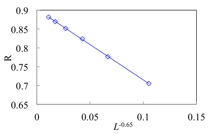
Here we add an observation about the scaling of the numbers and . From (1) and (2), we have the relation
| (6) |
and as a consequence we should expect that the quantity
| (7) |
converges to a constant for large , where is the number of sites in the system, which is for the geometry used here. Plotting this vs. , we see in Fig. 10 that we get a good straight line for , and that reaches a constant as . (Note here we used the periodic backbone—the black sites—for .) That goes to a constant provides further confirmation that the scaling relation (6) is valid.