跳到论文正文
W Papers独立论文阅读器 arXiv:1805.08132 论文正文 计算阅读时间 · 0%
引用这篇论文根据当前论文元数据生成,正式投稿前建议核对。


License: arXiv.org perpetual non-exclusive license
arXiv:1805.08132v2 [cond-mat.stat-mech] 23 Jul 2018

Overlap singularity and time evolution in integrable quantum field theory

D. X. Horváth Affiliation: BME "Momentum" Statistical Field Theory Research Group1111 Budapest, Budafoki út 8, Hungary Affiliation: Department of Theoretical Physics, Budapest University of Technology and Economics1111 Budapest, Budafoki út 8, Hungary    M. Kormos Affiliation: BME "Momentum" Statistical Field Theory Research Group1111 Budapest, Budafoki út 8, Hungary Affiliation: Department of Theoretical Physics, Budapest University of Technology and Economics1111 Budapest, Budafoki út 8, Hungary    G. Takács Affiliation: BME "Momentum" Statistical Field Theory Research Group1111 Budapest, Budafoki út 8, Hungary Affiliation: Department of Theoretical Physics, Budapest University of Technology and Economics1111 Budapest, Budafoki út 8, Hungary
6th July 2018
Abstract

We study homogeneous quenches in integrable quantum field theory where the initial state contains zero-momentum particles. We demonstrate that the two-particle pair amplitude necessarily has a singularity at the two-particle threshold. Albeit the explicit discussion is carried out for special (integrable) initial states, we argue that the singularity is inevitably present and is a generic feature of homogeneous quenches involving the creation of zero momentum particles. We also identify the singularity in quenches in the Ising model across the quantum critical point, and compute it perturbatively in phase quenches in the quantum sine–Gordon model which are potentially relevant to experiments. We then construct the explicit time dependence of one-point functions using a linked cluster expansion regulated by a finite volume parameter. We find that the secular contribution normally linear in time is modified by a t​ln⁡tt\ln t term. We additionally encounter a novel type of secular contribution which is shown to be related to parametric resonance. It is an interesting open question to resum the new contributions and to establish their consequences directly observable in experiments or numerical simulations.

1 Introduction

Understanding the out-of-equilibrium dynamics of isolated quantum many-body systems is one of the most challenging problems in contemporary physics. Due to the direct insight into quantum statistical physics provided by the experimental realisability of closed quantum systems, significant progress has been made both on the experimental and theoretical side in the study of non-equilibrium behaviour. Using cold atomic gases it has become possible to engineer and manipulate isolated quantum systems [1, 2, 3, 4, 5, 6, 7, 8, 9], and recent studies have led to a series of interesting discoveries such as the experimental observation of the lack of thermalisation in quantum integrable systems [1, 2, 3, 10].

A paradigmatic framework for studying non-equilibrium dynamics is provided by quantum quenches [11] which correspond to a sudden change of some parameters of a system prepared in an equilibrium state, typically in its ground state. For a long time, the focus of the theoretical investigations was the description of the late time asymptotic steady state. To explain the stationary state of integrable quantum systems, the concept of the generalised Gibbs ensemble (GGE) was proposed [12] and later experimentally confirmed [4]. However, specifying the complete set of conserved charges for the GGE in interacting integrable models proved to be a non-trivial problem [13, 14, 15, 16, 17, 18, 19] .

Beyond the steady state it is also of interest to describe the actual time evolution and identify universal features of the non-equilibrium dynamics. Theoretical description of the out-of-equilibrium time evolution is much more difficult and less understood than the characterisation of the steady state, and analytical results have mainly been obtained in systems that can be mapped to free particles [20, 21, 22, 23, 24, 25, 26, 27, 28, 29, 30, 31, 32, 33, 34] and in conformal field theory [11] and in a few cases in interacting integrable systems [35, 36, 37, 38, 39, 40, 41].

Quantum field theory (QFT) provides an effective and universal description of quantum systems near their critical point. Therefore small quenches in the vicinity of the critical point are expected to be described by a non-equilibrium QFT, capturing universal physics even out of equilibrium. Quenches in quantum field theories, on the other hand, are interesting also in their own right being relevant to high energy physics, and for certain experiments as well [42, 43].

In suitably small quantum field theory quenches, the semi-classical approach [44, 45, 46, 47] and approaches based on form factor expansions [48, 49, 50, 51, 52] lead to analytical predictions for the time evolution of certain observables. Whereas the perturbative approach in [51, 52] can be applied to any quench in which the pre-quench Hamiltonian is integrable, analytical results have only been obtained by perturbation theory up to first order in the quench amplitude. The method developed in [47, 48, 49, 50] can be applied whenever the post-quench Hamiltonian is integrable and the post-quench particle density is suitably small. This latter approach also requires to consider specific, so-called integrable quenches, for which the initial state can be cast in a squeezed coherent form in the post-quench basis as

|Ω⟩=𝒩​exp⁡(∫d​ϑ4​π​Ka​b​(ϑ)​Za†​(−ϑ)​Zb†​(ϑ))​|0⟩,|\Omega\rangle=\mathcal{N}\exp\left(\int\frac{d\vartheta}{4\pi}K_{ab}(\vartheta)Z_{a}^{\dagger}(-\vartheta)Z_{b}^{\dagger}(\vartheta)\right)|0\rangle\;, (1.1)

written in terms of the post-quench Faddeev-Zamolodchikov creation operators Za†​(ϑ)Z_{a}^{\dagger}(\vartheta) for particle species aa, the post-quench vacuum |0⟩|0\rangle and the pair-amplitude Ka​bK_{ab}, which we will often refer to simply as the KK function. It must be stressed that, for models with one particle species as well as for the repulsive regime of the sine–Gordon model, the smallness of the quench essentially guarantees the structure of (1.1), whereas for a generic quench protocol in a generic integrable QFT it is not known and probably not true [52, 53] that the initial state obeys this particular structure in the post-quench basis. For interacting integrable field theories, the determination of the KK function for a specific quench protocol assumed to be integrable is a difficult and unsolved problem, with some progress in the numerical determination [53, 54] and analytic approximations based on form factors [55, 56].

Nevertheless, integrable quenches are known to exist for lattice spin systems [57], and are an ideal starting point for analytic considerations in field theory due to their close resemblance to the integrable boundary states introduced by Ghoshal and Zamolodchikov [58]. In fact, following the case of boundary states it is possible to extend (1.1) with zero-momentum particles yielding

  • |Ω⟩=𝒩​exp⁡(ga2​Za†​(0)+∫d​ϑ4​π​Ka​b​(ϑ)​Za†​(−ϑ)​Zb†​(ϑ))​|0⟩,|\Omega\rangle=\mathcal{N}\exp\left(\frac{g_{a}}{2}Z_{a}^{\dagger}(0)+\int\frac{d\vartheta}{4\pi}K_{ab}(\vartheta)Z_{a}^{\dagger}(-\vartheta)Z_{b}^{\dagger}(\vartheta)\right)|0\rangle\;, (1.2)

where gag_{a} is called the one-particle coupling which corresponds to the quench breaking (particle number) parity. Such an initial state is also motivated by experiments [43] which show the presence of oscillations with a frequency corresponding to the energy of the zero-momentum particle (i.e. the particle mass).

For an initial state (1.2), time evolution of the vertex operator ei​β​ϕ/2e^{i\beta\phi/2} in the attractive regime of the sine–Gordon model was studied in [50]. In the homogeneous (translationally invariant) quenches considered here, the presence of zero-momentum solitons or antisolitons is excluded if the initial state is annihilated by the topological charge which is a typical situation including e.g quenches by local operators starting from the ground state of the model with a different coupling. For stationary breathers BnB_{n}, however, the one-particle couplings gBng_{B_{n}} can appear in (1.2). The conclusion of [50] was that one-particle oscillations of time dependence e−i​m​te^{-imt} show an exponential decay with several relaxation rate contributions. In particular, with only one breather species in the model the contribution of the first breather to the relaxation rate of one-particle oscillations is

τB1−1=mB1π​∫0∞d​ϑ​(1−SB1​B1​(ϑ))​|KB1​B1​(ϑ)|2​sinh⁡ϑ.\tau_{B_{1}}^{-1}=\frac{m_{B_{1}}}{\pi}\int_{0}^{\infty}d\vartheta\left(1-S_{B_{1}B_{1}}(\vartheta)\right)\left|K_{B_{1}B_{1}}(\vartheta)\right|^{2}\sinh\vartheta\;. (1.3)

For boundary field theories, however, it is known that the existence of a one-particle coupling implies a first order pole in the corresponding KK function at the origin,

Ka​a​(ϑ)∝−i​ga22​1ϑ;K_{aa}(\vartheta)\propto-i\frac{g_{a}^{2}}{2}\frac{1}{\vartheta}\ ; (1.4)

the correct relation of the residue to the one-particle coupling was first found in [59] and later proven in [60]. In this paper we show that this relation extends to the case of integrable quenches corresponding to an initial state of the form (1.2) as well. As an immediate consequence, the integral in (1.3) becomes divergent since SB1​B1​(0)=−1S_{B_{1}B_{1}}(0)=-1 . Even though much of the derivation in [50] remains valid, the singular expressions clearly need to be corrected.

In this paper we first demonstrate the presence of the singularity (1.4) whenever a zero-momentum particle is present in the initial state. Starting from this observation, we follow a linked cluster expansion similar to the one performed in [48, 49, 50] but now supported by a finite volume regularisation to treat the singularities and compute the time dependence of one-point functions ⟨𝒪⁡(t)⟩\langle\mathcal{O}(t)\rangle up to terms containing five particles focusing on the one-particle oscillations e−i​m​te^{-imt}. As a result of these calculations, we show that the linearly time dependent secular contribution in [50] is modified by a m​t​ln⁡m​tmt\ln mt term and a novel type of secular term is encountered which has analogies with the phenomenon of parametric resonance.

The detailed structure of our paper is the following. In Section 2, first a general argument is presented for the existence of the singularity (1.4), and then we consider two particular quench protocols that illustrate our arguments. In the Ising model, quenches from the ferromagnetic to the paramagnetic phase are discussed and the singular structure of the KK function is explicitly demonstrated in the continuum limit. Then we consider a quench protocol in the sine–Gordon model which consists of shifting the field by a constant. Computing the quench overlaps using an expansion in the quench magnitude, we demonstrate explicitly that the pair amplitude for the first breather possesses the anticipated singularity up to leading order. In Section 3 we perform a linked cluster expansion for the time-dependent one-point function, using a finite volume regularisation which was first introduced in [61]. This allows us to refine the argument for the existence of the singularity (1.4), and also the explicit construction of the contributions for ⟨𝒪⁡(t)⟩\langle\mathcal{O}(t)\rangle up to four particle terms, from which the terms corresponding to one-particle oscillations are extracted. We then consider the five-particle terms, but only present the leading order emergent secular contributions. In Section 4 we collect and present our formulas describing the time evolution, address the question of resummation in the linked cluster expansion and generalise our results to cases involving more than one particle species. Finally we discuss a class of secular terms linked to a mechanism analogous to parametric resonance, and conclude in Section 5. Due to the large amount of tedious calculations involved, most of their details are relegated to appendices. In Appendix A, the finite volume formalism is reviewed, while Appendices B and C are devoted to the quenches in the Ising and sine–Gordon models. The technical details of the linked cluster expansion and the calculation of the time evolution can be found in Appendices D, E, G, H and I. To confirm the validity of our calculations they were numerically cross-checked at several points; details of these checks are presented in Appendix J.

2 Integrable quenches with one-particle coupling and the singularity of KK

In this section we show that in integrable quenches with non-zero one-particle coupling gg the KK function necessarily possesses a first order pole of the form (1.4) at the origin. For simplicity, we focus on models with one particle species but the argument carries over to systems with several particle species. First we present a general argument based on an analogy with the one-point functions of bulk operators in the presence of boundaries discussed in [62]. The core of the argument is based on the cancellation of divergent terms in the expectation value which is evaluated using finite volume regulators. We then proceed to a concrete example of the quench in the Ising field theory crossing the phase boundary, and discuss an interesting quench in the sine–Gordon model, for which the one-particle coupling and the singular part of the KK function can be calculated to lowest order in the quench parameter and the presence of the singularity in KK and the relation of its residue to gg can be verified explicitly.

2.1 Boundary one-point functions

In the following we briefly review the boundary problem discussed in [62]. Let us consider an integrable field theory with a single massive particle constrained on a finite line x∈[0,ℛ]x\in[0,\mathcal{R}] with integrable boundary conditions α\alpha and β\beta at the two ends; for simplicity we consider the case when the left/right boundary conditions are identical i.e. α=β=B\alpha=\beta=B. The vacuum expectation value

⟨𝒪⁡(x)⟩B\langle\mathcal{O}(x)\rangle^{B} (2.1)

taken with respect to the ground state of the finite volume Hamiltonian HℛBH_{\mathcal{R}}^{B} can be rewritten using an Euclidean rotation

⟨𝒪⁡(x)⟩B=⟨B|e−H​x​𝒪​(0)​e−H⁡(ℛ−x)|B⟩⟨B|e−H​ℛ|B⟩,\langle\mathcal{O}(x)\rangle^{B}=\frac{\langle B|\ e^{-Hx}\mathcal{O}(0)\ e^{-H(\mathcal{R}-x)}\>|B\rangle}{\langle B|e^{-H\mathcal{R}}|B\rangle}\;, (2.2)

where the coordinate xx plays the role of the Euclidean time variable, HH is the infinite volume Hamiltonian in the crossed channel and |B⟩|B\rangle is the boundary state corresponding to the boundary condition BB. When the boundary state contains zero-momentum particles associated with a non-zero coupling of a single particle state to the boundary in the original channel, |B⟩|B\rangle can be expanded in the asymptotic multi-particle basis [58] as

|B⟩=𝒩​exp⁡(g¯B​Z†​(0)+∫d​ϑ4​π​KB​(ϑ)​Z†​(−ϑ)​Z†​(ϑ))​|0⟩,|B\rangle=\mathcal{N}\exp\left(\bar{g}_{B}Z^{\dagger}(0)+\int\frac{d\vartheta}{4\pi}K_{B}(\vartheta)Z^{\dagger}(-\vartheta)Z^{\dagger}(\vartheta)\right)|0\rangle\;, (2.3)

where for simplicity we assumed that the model has only one species,

KB​(ϑ)=RB​(i​π/2−ϑ)K_{B}(\vartheta)=R_{B}(i\pi/2-\vartheta)

in terms of the boundary reflection factor RB​(ϑ)R_{B}(\vartheta), and Z†​(ϑ)Z^{\dagger}(\vartheta) are the Faddeev–Zamolodchikov creation operators satisfying the commutation relations

Z†​(ϑ1)​Z†​(ϑ2)=S⁡(ϑ1−ϑ2)​Z†​(ϑ2)​Z†​(ϑ1).Z^{\dagger}(\vartheta_{1})Z^{\dagger}(\vartheta_{2})=S(\vartheta_{1}-\vartheta_{2})Z^{\dagger}(\vartheta_{2})Z^{\dagger}(\vartheta_{1})\;.

g¯B\bar{g}_{B} is the one-particle coupling to the boundary and the amplitudes KB​(ϑ)K_{B}(\vartheta) satisfy the boundary crossing-unitary equation [58]

KB​(ϑ)=S⁡(2​ϑ)​KB​(−ϑ),K_{B}(\vartheta)=S(2\vartheta)K_{B}(-\vartheta)\;,

which serves as a consistency relation of (2.3) and also implies KB​(ϑ)∗=KB​(−ϑ)K_{B}(\vartheta)^{*}=K_{B}(-\vartheta). The single particle coupling implies a pole for the reflection factor

RB​(ϑ)∼i2​gB2θ−i​π/2,R_{B}(\vartheta)\sim\frac{i}{2}\frac{g_{B}^{2}}{\theta-i\pi/2}\;,

which then yields a pole at the origin

KB​(ϑ)∼−i2​gB2ϑ,K_{B}(\vartheta)\sim-\frac{i}{2}\frac{g_{B}^{2}}{\vartheta}\;, (2.4)

for the boundary KK function. Whereas it was argued that g¯B=gB\bar{g}_{B}=g_{B} in [58], it was later demonstrated in [59, 63] that the proper normalisation is g¯B=gB/2\bar{g}_{B}=g_{B}/2, with a general proof given in [60].

The relation between the residue of KK and the boundary one-particle coupling is crucial for the consistency of a number of theoretical constructs, such as the boundary form factor bootstrap considered in [64]. For the one-point function, the approach of [62] is to put the theory in a finite volume LL in the crossed channel (with periodic boundary conditions) and consider the limit

⟨𝒪⁡(x)⟩B=limL→∞⟨𝒪⁡(x)⟩LB=limL→∞⟨BL|e−HL​x​𝒪​(0)​e−HL​(ℛ−x)|BL⟩⟨BL|e−HL​ℛ|BL⟩,\langle\mathcal{O}(x)\rangle^{B}=\lim_{L\to\infty}\langle\mathcal{O}(x)\rangle_{L}^{B}=\lim_{L\to\infty}\frac{\langle B_{L}|\ e^{-H_{L}x}\mathcal{O}(0)\ e^{-H_{L}(\mathcal{R}-x)}\ |B_{L}\rangle}{\langle B_{L}|e^{-H_{L}\mathcal{R}}|B_{L}\rangle}\;, (2.5)

where HLH_{L} is the finite volume Hamiltonian with periodic boundary conditions and |BL⟩|B_{L}\rangle represents the boundary state in finite volume. The finite volume is introduced here as a regulator for disconnected contributions arising from the matrix elements of the operator 𝒪\mathcal{O} which appear once |BL⟩|B_{L}\rangle is expanded in terms of the corresponding finite volume multi-particle eigenstates of HLH_{L}. The disconnected terms lead to positive powers of the dimensionless volume variable m​LmL which only cancel if the singularity of KBK_{B} is exactly as in (2.4). Therefore the singularity of KBK_{B} and the relation of its residue to the one-particle coupling are consistency criteria for the existence of well-defined one-point functions in the infinite volume theory.

The time evolution of the expectation value of a local operator 𝒪\mathcal{O} after a quantum quench with initial state

|Ω⟩=𝒩​exp⁡(g2​Z†​(0)+∫d​ϑ4​π​K​(ϑ)​Z†​(−ϑ)​Z†​(ϑ))​|0⟩,|\varOmega\rangle=\mathcal{N}\exp\left(\frac{g}{2}Z^{\dagger}(0)+\int\frac{d\vartheta}{4\pi}K(\vartheta)Z^{\dagger}(-\vartheta)Z^{\dagger}(\vartheta)\right)|0\rangle\;,

and post-quench Hamiltonian HH is given by the expression

⟨𝒪⁡(t)⟩=⟨Ω|ei​t​H​𝒪​(0)​e−i​t​H|Ω⟩⟨Ω|Ω⟩,\langle\mathcal{O}(t)\rangle=\frac{\langle\varOmega|\ e^{itH}\mathcal{O}(0)\ e^{-itH}|\varOmega\rangle}{\langle\varOmega|\varOmega\rangle}\;,

which is just a real time analogue of the boundary expectation value. The only difference is that the KK function appearing in |Ω⟩|\varOmega\rangle is not related to any reflection factor; in fact, Ghoshal–Zamolodchikov boundary states are not normalisable, while for quench initial states the factor 𝒩\mathcal{N} is chosen to ensure ⟨Ω|Ω⟩=1\langle\varOmega|\varOmega\rangle=1. However, it is clear from the calculations performed in [62] that the condition for the cancellation of singularities in unaffected by these details, therefore a well-defined expectation value ⟨𝒪⁡(t)⟩\langle\mathcal{O}(t)\rangle after an integrable quench with one-particle coupling g/2g/2, the KK function must have a first order pole at the origin with a residue equal to −ig2/2-ig^{2}/2.

In the next subsections we discuss two examples where this relation can be verified explicitly, while in Section 3 we consider the real time evolution and show that this condition must hold for consistency.

2.2 Quench in the Ising field theory from the ferromagnetic to the paramagnetic phase

In this subsection we study the Ising field theory and quenches across the two phases of the model, as in the Ising model only quenches from the ferromagnetic to the paramagnetic (PM) phase can account for a zero-momentum particle in the initial state. In our approach, we perform the continuum limit of various quantities obtained in the lattice model and in particular, we show that the pair-amplitude possesses a pole with the residue expected from the above considerations.

Quenches in the lattice model were discussed in [25, 26, 27] and for particular quenches within the ferromagnetic phase, calculations also in the continuum model [48] were performed and numerically checked [65]. Although for the F​M→P​MFM\rightarrow PM quench such calculations in the QFT were not carried out, the scaling limit of the analogous quantities in the lattice model make perfect sense, which we regard as the characteristics of the QFT quench problem. Throughout the subsection, we only discuss the most important features and formulas, and for a more detailed treatment of the topic, Appendix B is recommended to consult.

We first recall, that the transverse field quantum Ising model (TQIM) is defined by the Hamiltonian

H=−J∑i=1N(σixσi+1x+hσiz),H=-J\sum_{i=1}^{N}\left(\sigma_{i}^{x}\sigma_{i+1}^{x}+h\sigma_{i}^{z}\right)\;, (2.6)

where σiα\sigma_{i}^{\alpha} denotes the Pauli matrices at site ii, J>0J>0, hh is the transverse field and the boundary conditions are assumed to be periodic. By applying the Jordan–Wigner transformation, the Hamiltonian (2.6) can be mapped to spinless Majorana fermions with dispersion relation [66, 67]

εh​(k)=2​J​1+h2−2​h​cos⁡k,\varepsilon_{h}(k)=2J\sqrt{1+h^{2}-2h\cos k}\;, (2.7)

and with an energy gap Δ=2​J​|1−h|\Delta=2J|1-h|. The model possesses a quantum critical point at h=1h=1 separating the paramagnetic or disordered phase for h>1h>1 and the ferromagnetic, ordered phase for h<1h<1. In the disordered phase, the expectation value of σix\sigma_{i}^{x}, i.e. that of the magnetisation operator vanishes, while in the ferromagnetic phase its value is non-zero. The Hilbert space of the model consists of two sectors with respect to fermion number parity. In the Neveu–Schwarz and Ramond sectors states with even and odd number of fermions are present, respectively, resulting in the quantisation condition for the wave numbers

kn=2​πN​(n+12)Neveu–Schwarzpn=2​πN​nRamond,\begin{split}k_{n}=&\frac{2\pi}{N}\left(n+\frac{1}{2}\right)\quad\text{Neveu\textendash Schwarz}\\ p_{n}=&\frac{2\pi}{N}n\qquad\qquad\quad\text{Ramond}\;,\end{split} (2.8)

where nn is a positive integer.

Performing a quench in the transverse field hh, the pre- and post-quench excitations can be related via a Bogoliubov transformation if the initial state is the pre-quench vacuum. As a consequence, the squeezed-coherent form of the initial state in the post quench basis (1.1) is guaranteed. Focusing on quenching from the ground state of the FM phase to the PM phase, ( h0→hh_{0}\rightarrow h with h0<1h_{0}<1 and h>1h>1), one can write [25, 26, 27]

|0,h0⟩N​SF​M±|0,h0⟩RF​M2=12​NN​Sexp(i∑k⊂N​SK(k)a−k†ak†)|0,h⟩N​SP​M±12​NRexp(i∑p⊂R∖{0}K(p)a−p†ap†)a0†|0,h⟩RP​M,\begin{split}\frac{|0,h_{0}\rangle_{NS}^{FM}\pm|0,h_{0}\rangle_{R}^{FM}}{\sqrt{2}}=&\frac{1}{\sqrt{2}N_{NS}}\exp\left(i\sum_{k\subset NS}K(k)a_{-k}^{\dagger}a_{k}^{\dagger}\right)|0,h\rangle_{NS}^{PM}\\ \pm&\frac{1}{\sqrt{2}N_{R}}\exp\left(i\sum_{p\subset R\setminus\{0\}}K(p)a_{-p}^{\dagger}a_{p}^{\dagger}\right)a_{0}^{\dagger}|0,h\rangle_{R}^{PM}\;,\end{split} (2.9)

where NN​SN_{NS} and NRN_{R} are normalisation constants

NR2=∏n⊂ℕ+(1+|K⁡(2​πL​n)|2),NN​S2=∏m⊂ℕ+12(1+|K⁡(2​πL​m)|2),\begin{split}N_{R}^{2}=&\prod_{n\subset\mathbb{N}^{+}}\left(1+\left|K\left(\frac{2\pi}{L}n\right)\right|^{2}\right)\;,\\ N_{NS}^{2}=&\prod_{m\subset\mathbb{N}+\frac{1}{2}}\left(1+\left|K\left(\frac{2\pi}{L}m\right)\right|^{2}\right)\;,\end{split} (2.10)

aka_{k} and ak†a_{k}^{\dagger} are fermionic operators and KK can be found in Appendix B in (B.8).

In the scaling limit of the TQIM, JJ is sent to infinity together with h→1h\rightarrow 1 such that the gap associated with the fermion mass remains finite

M=2​J​|1−h|.M=2J|1-h|\;. (2.11)

In addition, the lattice spacing is sent to zero as a=12​Ja=\frac{1}{2J}. In particular, for the F​M→P​MFM\rightarrow PM quench, we send δ​h→0\delta h\rightarrow 0 in the following way:

h=1+δ​h,h0=1−M0M​δ​h,J=M2​δ​h,a=δ​hM,\begin{split}h=1+\delta h\;,\quad&h_{0}=1-\frac{M_{0}}{M}\delta h\;,\\ J=\frac{M}{2\delta h}\;,\quad&a=\frac{\delta h}{M}\;,\end{split} (2.12)

which ensures that the dispersion relation in the post- and pre-quench model is εh​(p​a)→M2+p2\varepsilon_{h}(pa)\rightarrow\sqrt{M^{2}+p^{2}} and εh0​(p​a)→M02+p2\varepsilon_{h_{0}}(pa)\rightarrow\sqrt{M_{0}^{2}+p^{2}} respectively, i.e. the mass in the PM and FM phase is MM and M0M_{0}. Upon the substitution k=p​ak=pa, the continuum limit of the square of the lattice KK function (B.8) in (2.9) is

|K⁡(p)|2=p2+M2​p2+M02−p2+M​M0p2+M2​p2+M02+p2−M​M0.|K(p)|^{2}=\frac{\sqrt{p^{2}+M^{2}}\sqrt{p^{2}+M_{0}^{2}}-p^{2}+MM_{0}}{\sqrt{p^{2}+M^{2}}\sqrt{p^{2}+M_{0}^{2}}+p^{2}-MM_{0}}\;. (2.13)

From (2.13) it is easily seen that this function has a 1/p21/p^{2} singularity at the origin with the coefficient

4​M02​M2(M+M0)2.\frac{4M_{0}^{2}M^{2}}{(M+M_{0})^{2}}\;.

This singularity corresponds to the presence of a zero-momentum particle in the Ramond contribution to the initial state (2.9). As p=M​sinh⁡ϑp=M\sinh\vartheta, the coefficient of the singularity of |K⁡(p)|2|K(p)|^{2} equals g44​M2\frac{g^{4}}{4}M^{2} , therefore K⁡(ϑ)K(\vartheta) can be written in the form (1.4) with

g=2​M0M+M0.g=2\sqrt{\frac{M_{0}}{M+M_{0}}}\;. (2.14)

Now we show that the one-particle coupling expressed with MM and M0M_{0} in (2.9) equals gg. To calculate the latter, we put the theory into finite volume, where (cf. also Section 3) the finite volume expansion of the integrable initial state reads

|Ω⟩L=𝒢(L)(|0⟩L+g2M​L|{0}⟩L+∑IK(ϑ)N2(ϑ,L)|{−I,I}⟩L.+…),|\Omega\rangle_{L}=\mathcal{G}(L)\left(|0\rangle_{L}+\frac{g}{2}\sqrt{ML}|\{0\}\rangle_{L}+\sum_{I}K(\vartheta)N_{2}(\vartheta,L)|\{-I,I\}\rangle_{L}.+...\right){\color[rgb]{0,0,0}{\color[rgb]{1,0,0}\>{\color[rgb]{0,0,0},}}} (2.15)

where the II denote quantum numbers labelling the finite volume states and N2N_{2} can be found in (A.6). Then from (2.9)

M​L​g2=NN​SNR,\sqrt{ML}\frac{g}{2}=\frac{N_{NS}}{N_{R}}\>, (2.16)

must hold. It is convenient to calculate the logarithm of their ratio:

ln⁡NN​S2NR2=ln∏n⊂ℕ+1+|K⁡(2​πL​(n−1/2))|21+|K⁡(2​πL​(n))|2,\begin{split}\ln\frac{N_{NS}^{2}}{N_{R}^{2}}=&\ln\prod_{n\subset\mathbb{N}^{+}}\frac{1+\left|K\left(\frac{2\pi}{L}(n-1/2)\right)\right|^{2}}{1+\left|K\left(\frac{2\pi}{L}(n)\right)\right|^{2}}\end{split}\;, (2.17)

which in Appendix B is shown to be equal to

ln⁡M​M0​L(M+M0)\ln\frac{MM_{0}L}{(M+M_{0})}

when L→∞L\rightarrow\infty, so (2.14) indeed holds.

2.3 Phase quenches in the sine–Gordon model

Consider the sine–Gordon model defined by the action

𝒜=∫d2​x​(12​∂μΦ​∂μΦ+μ2β2​cos⁡β​Φ),\mathcal{A}=\int d^{2}x\left(\frac{1}{2}\partial_{\mu}\Phi\partial^{\mu}\Phi+\frac{\mu^{2}}{\beta^{2}}\cos\beta\Phi\right)\>, (2.18)

in a finite volume LL with quasi-periodic boundary conditions

Φ⁡(t,x+L)=Φ⁡(t,x)+2​πβ​nn∈ℤ.\Phi(t,x+L)=\Phi(t,x)+\frac{2\pi}{\beta}n\quad n\in\mathbb{Z}\;.

The quench protocol consists of abruptly shifting the sine–Gordon field Φ→Φ+δ/β\Phi\rightarrow\Phi+\delta/\beta at t=0t=0, i.e. changing the phase of the cosine potential regarding the pre-quench vacuum as initial state for the post-quench evolution. The peculiarity of this protocol is that, as shown in Appendix C, it is possible to relate the pre- and post-quench ground states by a unitary transformation

|Ω⟩L=exp⁡(i​δβ​Π0)​|0⟩L,|\Omega\rangle_{L}=\exp\left(i\frac{\delta}{\beta}\Pi_{0}\right)|0\rangle_{L}\>, (2.19)

where

Π0=∫0Ld​x​Π​(t,x)=i​∫0L[H,Φ⁡(t,x)]​𝑑x\Pi_{0}=\int_{0}^{L}dx\Pi(t,x)=i\int_{0}^{L}[H,\Phi(t,x)]dx

is the zero mode of the conjugate momentum field Π=Φ˙\Pi=\dot{\Phi}. This allows one to derive a form factor expansion for the overlaps with an arbitrary state |χ⟩|\chi\rangle

⟨χ|Ω⟩LL=L⟨χ|exp(iδβΠ0)|0⟩L,\vphantom{O}{}_{L}\langle\chi|\Omega\rangle_{L}=\vphantom{O}_{L}\langle\chi|\exp\left(i\frac{\delta}{\beta}\Pi_{0}\right)|0\rangle_{L}\,, (2.20)

by expanding the exponential into power series,

L⟨χ|Ω⟩L=∑l=0∞(−1)ll!(δβ)l∑α1…∑αl−1∫(∏idxi)L⟨χ|ei​P^​x1Φ(0)e−i​P^​x1|α1⟩L(Eχ−Eα1)×L⟨α1|ei​P^​x2Φ(0)e−i​P^​x2|α2⟩L(Eα1−Eα2)…L⟨αl−1|ei​P^​xlΦ(0)e−i​P^​xl|0⟩L(Eαl−1−E0),\begin{split}\vphantom{O}{}_{L}\langle\chi|\Omega\rangle_{L}=\sum_{l=0}^{\infty}\frac{(-1)^{l}}{l!}\mbox{$\left({\displaystyle\frac{\delta}{\beta}}\right)$}^{l}\sum_{\alpha_{1}}\ldots\sum_{\alpha_{l-1}}\int\left(\prod_{i}dx_{i}\right)\vphantom{O}_{L}\langle\chi|e^{i\hat{P}x_{1}}\Phi(0)e^{-i\hat{P}x_{1}}|\alpha_{1}\rangle_{L}(E_{\chi}-E_{\alpha_{1}})\times\\ \vphantom{O}{}_{L}\langle\alpha_{1}|e^{i\hat{P}x_{2}}\Phi(0)e^{-i\hat{P}x_{2}}|\alpha_{2}\rangle_{L}(E_{\alpha_{1}}-E_{\alpha_{2}})...\vphantom{O}_{L}\langle\alpha_{l-1}|e^{i\hat{P}x_{l}}\Phi(0)e^{-i\hat{P}x_{l}}|0\rangle_{L}(E_{\alpha_{l-1}}-E_{0}),\end{split} (2.21)

where P^\hat{P} is the momentum operator and the αi\alpha_{i} index l−1l-1 complete sets of asymptotic multi-particle eigenstates. As the initial state is the ground state of a translational invariant Hamiltonian, the overlaps are non-zero only for states |χ⟩|\chi\rangle of total spatial momentum zero. Due to the integrals over xi,x_{i}, this also restricts the intermediate states |αi⟩L|\alpha_{i}\rangle_{L} to have zero total momentum so we can write

⟨χ|Ω⟩LL=\vphantom{O}{}_{L}\langle\chi|\Omega\rangle_{L}= ∑l=0∞(−1)l(δβ)lLll!∑α1~…∑αl−1~L⟨χ|Φ(0)|α1⟩L(Eχ−Eα1)×\displaystyle\sum_{l=0}^{\infty}(-1)^{l}\mbox{$\left({\displaystyle\frac{\delta}{\beta}}\right)$}^{l}\frac{L^{l}}{l!}\tilde{\sum_{\alpha_{1}}}\ldots\tilde{\sum_{\alpha_{l-1}}}\vphantom{O}_{L}\langle\chi|\Phi(0)|\alpha_{1}\rangle_{L}(E_{\chi}-E_{\alpha_{1}})\times (2.22)
⟨α1|Φ(0)|α2⟩LL(Eα1−Eα2)…L⟨αl−1|Φ(0)|0⟩L(Eαl−1−E0),\vphantom{O}{}_{L}\langle\alpha_{1}|\Phi(0)|\alpha_{2}\rangle_{L}(E_{\alpha_{1}}-E_{\alpha_{2}})...\vphantom{O}_{L}\langle\alpha_{l-1}|\Phi(0)|0\rangle_{L}(E_{\alpha_{l-1}}-E_{0})\;, (2.23)

where the tildes over the sums mean that only zero momentum states are included.

We now compute the overlap for the first breather to first order in δ/β\delta/\beta. Matching the finite volume expression of the initial state (2.19) with the general case (2.15), and using (A.6) and the finite volume form factors (A.14), we obtain

m1​L​g2=L⟨{0}|Ω⟩L=−m1LδβL⟨{0}|Φ(0)|0⟩L=−(δβ)​m1​L​FB1∗m1​L,\begin{split}\sqrt{m_{1}L}\,\frac{g}{2}=&{}_{L}\langle\{0\}|\Omega\rangle_{L}\\ =&-m_{1}L{\displaystyle\frac{\delta}{\beta}}{}_{L}\langle\{0\}|\Phi(0)|0\rangle_{L}\\ =&-\mbox{$\left({\displaystyle\frac{\delta}{\beta}}\right)$}m_{1}L\frac{F_{B_{1}}^{*}}{\sqrt{m_{1}L}}\;,\end{split} (2.24)

from which

g2=−δβ​FB1∗,\frac{g}{2}=-\mbox{${\displaystyle\frac{\delta}{\beta}}$}F_{B_{1}}^{*}\;, (2.25)

where FB1F_{B_{1}} is the infinite volume one-breather form factor of Φ\Phi (C.11).

Since the form factors of Φ\Phi with even number of breathers B1B_{1} vanishes, the lowest non-trivial order for the pair amplitude KK is (δ/β)2\left(\delta/\beta\right)^{2} :

N2​(ϑ,L)​K​(ϑ)=L⟨{I,−I}|Ω⟩L=(δβ)2L22∑α1~L⟨{I,−I}|Φ(0)|α1⟩L(2m1coshϑ−Eα1)L⟨α1|Φ(0)|0⟩LEα1,\begin{split}N_{2}(\vartheta,L)K(\vartheta)=&{}_{L}\langle\{I,-I\}|\Omega\rangle_{L}\\ =&\mbox{$\left({\displaystyle\frac{\delta}{\beta}}\right)$}^{2}\frac{L^{2}}{2}\tilde{\sum_{\alpha_{1}}}{}_{L}\langle\{I,-I\}|\Phi(0)|\alpha_{1}\rangle_{L}(2m_{1}\cosh\vartheta-E_{\alpha_{1}}){}_{L}\langle\alpha_{1}|\Phi(0)|0\rangle_{L}E_{\alpha_{1}}\,,\end{split} (2.26)

where ϑ\vartheta is related to the quantum number II via the Bethe quantisation condition

m1​L​sinh⁡ϑ+δB1​B1​(2​ϑ)=2​π​I,m_{1}L\sinh\vartheta+\delta_{B_{1}B_{1}}(2\vartheta)=2\pi I\,, (2.27)

N2​(θ,L)N_{2}(\theta,L) is a finite volume normalisation factor (A.6) δB1​B1\delta_{B_{1}B_{1}} and its derivative φB1​B1​(ϑ)\varphi_{B_{1}B_{1}}(\vartheta) is defined by SB1​B1​(ϑ)=−ei​δB1​B1​(ϑ)S_{B_{1}B_{1}}(\vartheta)=-e^{i\delta_{B_{1}B_{1}}(\vartheta)}, and θ1,…,θn\theta_{1},...,\theta_{n} are the particle rapidities in the state |α1⟩L|\alpha_{1}\rangle_{L} determined by finite volume quantisation relations analogous to (2.27). Using the expression for finite volume form factors (A.14) it can be written as

(δβ)2L22∑n=1∞∑{β}nFB1​B1​Bi1​…​Bin​(i​π+ϑ,i​π−ϑ,θ1,…​θn)(m1​L​cosh⁡ϑ)2+(m1​L​cosh⁡ϑ)​φB1​B1​(ϑ)​ρn​(θ1,…​θn)×(2m1coshϑ−∑i=1nmicoshθi)FBi1​…​Bin∗(θ1,…θn)(∑i=1nmicoshθi).\begin{split}&\mbox{$\left({\displaystyle\frac{\delta}{\beta}}\right)$}^{2}\frac{L^{2}}{2}\sum_{n=1}^{\infty}\sum_{\{\beta\}_{n}}\frac{F_{B_{1}B_{1}B_{i_{1}}...B_{i_{n}}}(i\pi+\vartheta,i\pi-\vartheta,\theta_{1},...\theta_{n})}{\sqrt{\left(m_{1}L\cosh\vartheta\right)^{2}+\left(m_{1}L\cosh\vartheta\right)\,\varphi_{B_{1}B_{1}}(\vartheta)}\rho_{n}(\theta_{1},...\theta_{n})}\times\\ &\left(2m_{1}\cosh\vartheta-\sum_{i=1}^{n}m_{i}\cosh\theta_{i}\right)F_{B_{i_{1}}...B_{i_{n}}}^{*}(\theta_{1},...\theta_{n})\left(\sum_{i=1}^{n}m_{i}\cosh\theta_{i}\right)\,.\end{split} (2.28)

In Appendix C it is shown that in the limits L→∞L\rightarrow\infty and ϑ→0\vartheta\rightarrow 0 only the n=1n=1 term survives where the single particle in the intermediate state is also a B1B_{1}, from which

K⁡(ϑ)∼(δβ)2​FB1​B1​B1​(i​π+ϑ,i​π−ϑ,0)​(2​cosh⁡ϑ−1)​FB1*2​cosh⁡ϑ.K(\vartheta)\sim\mbox{$\left({\displaystyle\frac{\delta}{\beta}}\right)$}^{2}\frac{F_{B_{1}B_{1}B_{1}}(i\pi+\vartheta,i\pi-\vartheta,0)(2\cosh\vartheta-1)F_{B_{1}}^{\text{*}}}{2\cosh\vartheta}\,. (2.29)

Using the form factor kinematical singularity equation (A.12) one can extract that for small ϑ\vartheta

FB1​B1​B1​(i​π+ϑ,i​π−ϑ,0)∼−4​iϑ​FB1,F_{B_{1}B_{1}B_{1}}(i\pi+\vartheta,i\pi-\vartheta,0)\sim-\frac{4i}{\mathbf{\vartheta}}F_{B_{1}}\,, (2.30)

so

K⁡(ϑ)∼−2​i​(δβ​FB1)2​1ϑ+O⁡(ϑ0)=−i​g22​1ϑ+O⁡(ϑ0),\begin{split}K(\vartheta)\sim&-2i\left({\displaystyle\frac{\delta}{\beta}}F_{B_{1}}\right)^{2}\frac{1}{\vartheta}+O(\vartheta^{0})\\ =&-i\frac{g^{2}}{2}\frac{1}{\vartheta}+O(\vartheta^{0})\,,\end{split} (2.31)

where we used (2.25) which establishes the relation (2.4) between the one-particle coupling of the first breather and the singularity of its pair amplitude for this particular quench in the sine–Gordon model.

We remark that for this particular quench protocol we do not know whether it leads to an integrable initial state of the generalised squeezed form (1.2). However, we recall that the proof of the analogous relation in boundary quantum field theory presented in [60] does not depend on integrability either (in fact, it works in general D+1D+1 space-time dimensions).

Note also that the above argument straightforwardly generalises to a much larger class of quench protocols, the “exponential quenches” when the initial state is related to the post-quench ground state via

|Ω⟩L=exp⁡(i​λ​∫d​x​Ψ​(x))​|0⟩L,|\Omega\rangle_{L}=\exp\left(i\lambda\int dx\Psi(x)\right)|0\rangle_{L}\>, (2.32)

where Ψ⁡(x)\Psi(x) is a local field which breaks particle number parity.

3 Linked cluster expansion in finite volume

To describe the time evolution of expectation values of local operator, we follow the approach developed in [48, 49, 50] and apply a linked cluster expansion, combined with the finite volume regularisation scheme used in [62, 68]. The latter is based on the finite volume form factor formalism developed in [61]; the ingredients necessary for our calculations are described in Appendix A.

For a quench starting from an initial state written in terms of post-quench multi-particle states as in (1.2), a natural approach to compute the one-point function of a local operator 𝒪\mathcal{O} is to decompose into contributions from states with different number of particles, which results in an expansion in terms of form factors of the local operator. However, in infinite volume form factors possess pole singularities due to (A.12), and for quenches with one-particle coupling the KK functions also possess singularities. As a result, the contributions are ill-defined and need to be regularised which can be done by putting the theory in finite volume, where due to the quantisation of the particle momenta neither the kinematic singularities of the form factors nor the singularities of the pair-amplitude contribute. The finite volume LL can be considered as a physical regulator and the expectation value is then written as

⟨𝒪⁡(t)⟩=⟨Ω|ei​t​H​𝒪​(0)​e−i​t​H|Ω⟩⟨Ω|Ω⟩=limL→∞L⟨Ω|ei​t​H𝒪(0)e−i​t​H|Ω⟩LL⟨Ω|Ω⟩L,\begin{split}\langle\mathcal{O}(t)\rangle=&\frac{\langle\varOmega|\ e^{itH}\mathcal{O}(0)\ e^{-itH}|\varOmega\rangle}{\langle\varOmega|\varOmega\rangle}\\ =&\lim_{L\rightarrow\infty}\frac{{}_{L}\langle\varOmega|\ e^{itH}\mathcal{O}(0)\ e^{-itH}|\varOmega\rangle_{L}}{{}_{L}\langle\varOmega|\varOmega\rangle_{L}}\;,\end{split} (3.1)

which is first evaluated for finite LL where one can verify the cancellation of singular terms explicitly and then take the limit L→∞L\rightarrow\infty.

To perform the calculation, one needs an expression for the initial state in finite volume which was derived in [62]:

|Ω⟩L=𝒢(L)(|0⟩L+g2m​L|{0}⟩L+∑IK(ϑ)N2(ϑ,L)|{−I,I}⟩L+∑Ig2K(ϑ)N3(ϑ,L)|{−I,I,0}⟩L+12∑I≠JK(ϑ1)K(ϑ2)N4(ϑ1,ϑ2,L)|{−I,I,−J,J}⟩L)+…,|\varOmega\rangle_{L}=\mathcal{G}(L)\Big(|0\rangle_{L}+\frac{g}{2}\sqrt{mL}|\{0\}\rangle_{L}+\sum_{I}K(\vartheta)N_{2}(\vartheta,L)|\{-I,I\}\rangle_{L}\\ +\sum_{I}\frac{g}{2}K(\vartheta)N_{3}(\vartheta,L)|\{-I,I,0\}\rangle_{L}+\frac{1}{2}\sum_{I\neq J}K(\vartheta_{1})K(\vartheta_{2})N_{4}(\vartheta_{1},\vartheta_{2},L)|\{-I,I,-J,J\}\rangle_{L}\Big)+\ldots\;, (3.2)

where I,JI,J are Bethe quantum numbers and we used the notations introduced in Appendix A. To simplify notations, one can write the following shorthand for

|Ω⟩L=𝒢⁡(L)​∑n=0∞|Ω⟩(n),|\varOmega\rangle_{L}=\mathcal{G}(L)\sum_{n=0}^{\infty}|\varOmega\rangle^{(n)}\;,

where |Ω⟩(0)=|0⟩L,|Ω⟩(1)=g2​N1​(L)​|{0}⟩L,|\varOmega\rangle^{(0)}=|0\rangle_{L}\;,|\varOmega\rangle^{(1)}=\frac{g}{2}N_{1}(L)|\{0\}\rangle_{L}\;, etc. denote the contributions with a fixed number of particles.

To ensure the convergence of the expansion for high energies one can introduce a regulator parameter RR and consider

⟨𝒪⁡(t,R)⟩=⟨Ω|e(−R2+i​t)​H​𝒪​(0)​e(−R2−i​t)​H|Ω⟩⟨Ω|e−R​H|Ω⟩,\langle\mathcal{O}(t,R)\rangle=\frac{\langle\varOmega|\ e^{\left(-\frac{R}{2}+it\right)H}\mathcal{O}(0)\ e^{\left(-\frac{R}{2}-it\right)H}|\varOmega\rangle}{\langle\varOmega|e^{-RH}|\varOmega\rangle}\;, (3.3)

where R>0R>0. When recasting the quantum number sums in terms of contour integrals, RR ensures that the integrals themselves are convergent and therefore allows appropriate manipulations of the contours. At the end of the calculation the parameter RR is sent to zero.

Following the procedure introduced in [69], one can separate contributions indexed by particle number as follows

Ck​l=(k)⟨Ω|e(−R2+i​t)​H𝒪(0)e(−R2−i​t)​H|Ω⟩(l),C_{kl}\,=\,^{(k)}\langle\varOmega|e^{\left(-\frac{R}{2}+it\right)H}\mathcal{O}(0)\ e^{\left(-\frac{R}{2}-it\right)H}|\varOmega\rangle^{(l)}\;,

and for a proper normalisation of the state one must also divide by the “partition function”

Z=∑nZn=∑n⟨Ω|e−R​H|Ω⟩L(n)L(n).Z=\sum_{n}Z_{n}=\sum_{n}{}_{L}^{(n)}\langle\varOmega|e^{-RH}|\varOmega\rangle_{L}^{(n)}\,.

In particular for ZZ, the first few terms are

Z0=1,Z1=g24​m​L​e−m​R,Z_{0}=1\;,\qquad\qquad Z_{1}=\frac{g^{2}}{4}mLe^{-mR}\;, (3.4)

and

Z2=∑IK∗​(ϑ)​K​(ϑ)​N2​(ϑ,L)2​e−2​m​R​cosh⁡ϑ.Z_{2}=\sum_{I}K^{*}(\vartheta)K(\vartheta)N_{2}(\vartheta,L)^{2}e^{-2mR\cosh\vartheta}\;. (3.5)

Let us turn to the issue of the expansion parameter. Whereas in our calculations RR is eventually sent to zero at the end, for ⟨𝒪⁡(t,R)⟩\langle\mathcal{O}(t,R)\rangle is expected to be well-defined for any finite RR. Therefore let us first treat RR as a large positive quantity, and introduce the parameters z=e−m⁡(R/2+i​t)z=e^{-m(R/2+it)} and z¯=e−m⁡(R/2−i​t)\bar{z}=e^{-m(R/2-it)}. Then the order of Ck​lC_{kl} is z¯k​zl\bar{z}^{k}z^{l} , and that of ZnZ_{n} is (z​z¯)n(z\bar{z})^{n}. The inverse of the partition function, thus can be expanded in powers of z​z¯z\bar{z} as

Z−1=∑nZ¯n,Z^{-1}=\sum_{n}\bar{Z}_{n}\;,

where the first few terms read

Z¯0=1,Z¯1=−Z1,Z¯2=Z12−Z2.\bar{Z}_{0}=1\;,\qquad\bar{Z}_{1}=-Z_{1}\;,\qquad\bar{Z}_{2}=Z_{1}^{2}-Z_{2}\;.

Putting these ingredients together, in a finite volume LL we obtain

⟨𝒪⁡(t,R)⟩L=1Z​∑Ck​l=∑D~k​l,\langle\mathcal{O}(t,R)\rangle_{L}=\frac{1}{Z}\sum C_{kl}=\sum\tilde{D}_{kl}\;, (3.6)

where analogously to to [62] and [69], D~n​m\tilde{D}_{nm} is introduced as

D~k​l=∑jCk−j,l−j​Z¯j,\tilde{D}_{kl}=\sum_{j}C_{k-j,l-j}\bar{Z}_{j}\;, (3.7)

with the first few terms having the form

D~1​l\displaystyle\tilde{D}_{1l} =C1​l−Z1​C0,l−1,\displaystyle=C_{1l}-Z_{1}C_{0,l-1}\;, l=1,2,…,\displaystyle l=1,2,\dots\;,
D~2​l\displaystyle\tilde{D}_{2l} =C2​l−Z1​C1,l−1+(Z12−Z2)​C0,l−2,\displaystyle=C_{2l}-Z_{1}C_{1,l-1}+(Z_{1}^{2}-Z_{2})C_{0,l-2}\;, l=2,3,….\displaystyle l=2,3,\dots\;.

Since the D~k​l\tilde{D}_{kl} are of order zk​z¯lz^{k}\bar{z}^{l}, they must separately be well-defined as L→∞L\to\infty:

Dk​l=limL→∞D~k​l,D_{kl}=\lim_{L\to\infty}\tilde{D}_{kl}\;, (3.8)

and so the infinite volume limit can be written as

⟨𝒪⁡(t,R)⟩=∑k,lDk​l.\langle\mathcal{O}(t,R)\rangle=\sum_{k,l}D_{kl}\;.

For convenience and later use, we also introduce the quantities

G~n=∑l=0nD~n−l,l,\tilde{G}_{n}=\sum_{l=0}^{n}\tilde{D}_{n-l,l}\;, (3.9)

whose infinite volume limit is denoted by GnG_{n}.

The expressions individual Ck​lC_{kl} contain finite volume form factors, which in general are given by [61]

L⟨{I1,…,Ik|O|{J1,…,Jl}⟩L=Fk+lO​(ϑ1+i​π,…,ϑk+i​π,ϑ1′,…,ϑl′)ρk​(ϑ1,…,ϑk)​ρl​(ϑ1′,…,ϑl′)+𝒪(e−μ​L),\begin{split}{}_{L}\langle\{I_{1},\dots,I_{k}|O|\{J_{1},\dots,J_{l}\}\rangle_{L}=\frac{F_{k+l}^{O}(\vartheta_{1}+i\pi,\dots,\vartheta_{k}+i\pi,\vartheta^{\prime}_{1},\dots,\vartheta^{\prime}_{l})}{\sqrt{\rho_{k}(\vartheta_{1},\dots,\vartheta_{k})\rho_{l}(\vartheta^{\prime}_{1},\dots,\vartheta^{\prime}_{l})}}+\mathcal{O}(e^{-\mu L})\;,\end{split} (3.10)

where it is understood that the rapidities {ϑ1,…,ϑk}\{\vartheta_{1},\dots,\vartheta_{k}\} and {ϑ1′,…,ϑl′}\{\vartheta^{\prime}_{1},\dots,\vartheta^{\prime}_{l}\} are solutions to the corresponding Bethe–Yang equations with quantum numbers {In},{Jn}\{I_{n}\},\{J_{n}\}. Formula (3.10) is valid whenever there are no coinciding rapidities; otherwise a more complicated formula taking into account disconnected contributions is necessary. In this paper we are interested in contributions to one-particle oscillations, for which coinciding rapidities cannot occur, the numbers of particles in the two multi-particle states differ by an odd number which excludes the two possible cases with disconnected terms (cf. [61]).

Note that the equality (3.10) is valid up to a suitably chosen phase factor which can be changed by redefining the phases of the finite volume eigenstates |{I1,…,In}⟩L|\{I_{1},\dots,I_{n}\}\rangle_{L}. This includes also the fact that the ordering of the particles is not determined by first principles and any exchange leads to an SS-matrix factor according to (A.10). It is clear that all such ambiguities cancel in the expectation value (3.3); however, for a practical calculation one must fix the phases of the multi-particle contributions to the matrix elements consistently. Here we make use of the consistent prescription introduced in [62]: any time the amplitudes K⁡(ϑi)K(\vartheta_{i}) and K∗​(ϑi)K^{*}(\vartheta_{i}) appear with some ϑi\vartheta_{i}, the explicit order of the rapidities substituted into the relevant form factor is given by (−ϑi,ϑi)(-\vartheta_{i},\vartheta_{i}) and (ϑi+i​π,−ϑi+i​π)(\vartheta_{i}+i\pi,-\vartheta_{i}+i\pi), respectively. Exchanging any two pairs of rapidities does not make any difference, therefore the phase of the form factors is completely fixed by the above rule. Note that the presence of zero-momentum particles does not produce any additional ambiguities.

3.1 The singularity of K revisited

Now we are ready to complete our arguments why the pair-amplitude must be singular in integrable quenches with one-particle coupling. Recall that in the boundary problem [62] the ordering of the terms was performed according to powers of e−m⁡(ℛ−x)e^{-m(\mathcal{R}-x)} and e−m​xe^{-mx}, which resulted in the same expressions for the boundary version of D~k​l\tilde{D}_{kl} that we obtained in (3.7) with the expansion parameters z=e−m⁡(R/2+i​t)z=e^{-m(R/2+it)} and z¯=e−m⁡(R/2−i​t)\bar{z}=e^{-m(R/2-it)}. In the boundary problem, the existence of the infinite volume limit (3.8) and eventually ⟨𝒪⁡(x)⟩B\langle\mathcal{O}(x)\rangle^{B} requires the presence of the singularity

KB​(ϑ)∼−i2​gB2ϑ,K_{B}(\vartheta)\sim-\frac{i}{2}\frac{g_{B}^{2}}{\vartheta}\;,

therefore

K⁡(ϑ)∼−i2​g2ϑK(\vartheta)\sim-\frac{i}{2}\frac{g^{2}}{\vartheta}

must hold for the quench problem as well. The easiest way to see that is to consider the one-particle contribution −Z1-Z_{1} which behaves as m​LmL. To make C12−Z1​C01C_{12}-Z_{1}C_{01} finite in the infinite volume limit, C12C_{12} must have a similar volume-dependence, which is ensured by the singularity of KK involved in C12C_{12}.

At the end of the calculations the regulator RR is sent to zero. The contribution GnG_{n} (3.9) is of order |z|n=(e−mR/2)n|z|^{n}=(e^{-mR/2})^{n} and just as in [62] it turns out that the coefficient of the largest power of the m​LmL term is always of order gng^{n} . Focussing on the behaviour of the singular term, the small parameter of the linked-cluster calculation can be identified with gg. As the singularity of the KK is of order g2g^{2} one can formally treat KK as a term of order g2g^{2}. This way of counting the orders results in the same classification of contributions D~k​l\tilde{D}_{kl} (3.9) that we obtained by considering zz and z¯\bar{z} as the expansion parameters.

This counting of orders is clearest for a perturbative quench corresponding to changing the Hamiltonian as

δ​H=λ​∫d​x​Ψ​(x),\delta H=\lambda\int dx\Psi(x)\;,

where Ψ\Psi is a purely odd operator (i.e. whose form factors with an even number of particles in the pre-quench system is zero). Using perturbation theory to compute the overlaps following [51, 52] one obtains that the one-particle coupling is of order λ\lambda, while the pair amplitude KK is always of order λ2.\lambda^{2}.

When the perturbing operator has even matrix elements as well, the pair-amplitude can also possess a λ\lambda order term. Whereas this term is not singular due to the regular behaviour of F⁡(i​π+ϑ,i​π−ϑ)F(i\pi+\vartheta,i\pi-\vartheta) at ϑ=0\vartheta=0, at order λ2\lambda^{2} a singular term similar to the one found in Section 2 is always present. Therefore the presence of the zero-rapidity pole singularity of KK is generic.

3.2 Contributions up to 4t​h4^{th} order: analytic continuation of the boundary result

In this section we present all the terms up to fourth order using the Euclidean quantities computed in [62] and continuing them to real time. The Euclidean one-point function

⟨𝒪⁡(x)⟩B=⟨B|e−H​x​𝒪​(0)​e−H⁡(R−x)|B⟩⟨B|e−H​R|B⟩=∑k,lDk​l\langle\mathcal{O}(x)\rangle^{B}=\frac{\langle B|\ e^{-Hx}\mathcal{O}(0)\ e^{-H(R-x)}\ |B\rangle}{\langle B|e^{-HR}|B\rangle}=\sum_{k,l}D_{kl} (3.11)

was computed up to contributions Dk​lD_{kl} with k+l≤4k+l\leq 4 which are collected in Appendix E.

For the analytic continuation, we apply the R→0R\rightarrow 0 and x→−i​tx\rightarrow-it substitutions together with KB→KK_{B}\rightarrow K and gB→gg_{B}\rightarrow g which give

G0:⟨0|𝒪|0⟩,G1:g​ℜ⁡e​F1𝒪​e−i​m​t,G2:g24​F2𝒪​(i​π,0)+ℜ⁡e​∫−∞∞d​θ2​π​K​(θ)​F2𝒪​(−ϑ,ϑ)​e−i​m​t​2​cosh⁡ϑ,G3:g2​ℜ⁡e​∫−∞∞d​ϑ2​π​K​(ϑ)​F3𝒪​(−ϑ,ϑ,0)​e−i​m​t​(2​cosh⁡ϑ+1),+g2ℜe∫−∞∞d​ϑ2​π{K(ϑ)F3𝒪(iπ,−ϑ,ϑ)e−i​m​t​(2​cosh⁡ϑ−1)−2g2cosh⁡ϑsinh2⁡ϑF1𝒪e−i​m​t}+2​g3​φ​(0)​ℜ⁡e​F1𝒪​e−i​m​t,\begin{split}G_{0}:\quad&\langle 0|\mathcal{O}|0\rangle\quad,\\ G_{1}:\quad&g\,\Re eF_{1}^{\mathcal{O}}e^{-imt},\\ G_{2}:\quad&\frac{g^{2}}{4}F_{2}^{\mathcal{O}}(i\pi,0)+\Re e\int_{-\infty}^{\infty}\frac{d\theta}{2\pi}K(\theta)F_{2}^{\mathcal{O}}(-\vartheta,\vartheta)e^{-imt2\cosh\vartheta}\;,\\ G_{3}:\quad&\frac{g}{2}\Re e\int_{-\infty}^{\infty}\frac{d\vartheta}{2\pi}K(\vartheta)F_{3}^{\mathcal{O}}(-\vartheta,\vartheta,0)e^{-imt\left(2\cosh\vartheta+1\right)}\;,\\ &+\frac{g}{2}\Re e\int_{-\infty}^{\infty}\frac{d\vartheta}{2\pi}\left\{K(\vartheta)F_{3}^{\mathcal{O}}(i\pi,-\vartheta,\vartheta)e^{-imt\left(2\cosh\vartheta-1\right)}-2g^{2}\frac{\cosh\vartheta}{\sinh^{2}\vartheta}F_{1}^{\mathcal{O}}e^{-imt}\right\}\\ &+2g^{3}\varphi(0)\Re eF_{1}^{\mathcal{O}}e^{-imt}\;,\end{split} (3.12a)
G4:14ℜe∫−∞∞d​ϑ12​πd​ϑ22​πK(ϑ1)K(ϑ2)F4𝒪(−ϑ1,ϑ1,−ϑ2,ϑ2)e−imt(2coshϑ1+2coshϑ2)+g24ℜe∫−∞∞d​ϑ2​πK(ϑ)F4𝒪(−ϑ+iπ,ϑ+iπ,iπ,0)e−i​m​t​2​cosh⁡ϑ+14∫−∞∞d​ϑ12​πd​ϑ22​πK(ϑ1)K(ϑ2)F4𝒪(iπ−ϑ1iπ+ϑ1,−ϑ2,ϑ2)ei​m​t​2​(cosh⁡ϑ1−cosh⁡ϑ2)+F2𝒪(iπ,0)∫−∞∞d​ϑ2​π{|K(ϑ)|2−g4​cosh⁡ϑ4​sinh2⁡ϑ}+g48​F2𝒪​(i​π,0)​φ​(0),\begin{split}G_{4}:\quad&\frac{1}{4}\Re e\int_{-\infty}^{\infty}\frac{d\vartheta_{1}}{2\pi}\frac{d\vartheta_{2}}{2\pi}K(\vartheta_{1})K(\vartheta_{2})F_{4}^{\mathcal{O}}(-\vartheta_{1},\vartheta_{1},-\vartheta_{2},\vartheta_{2})e^{-imt\left(2\cosh\vartheta_{1}+2\cosh\vartheta_{2}\right)}\\ &+\frac{g^{2}}{4}\Re e\int_{-\infty}^{\infty}\frac{d\vartheta}{2\pi}K(\vartheta)F_{4}^{\mathcal{O}}(-\vartheta+i\pi,\vartheta+i\pi,i\pi,0)e^{-imt2\cosh\vartheta}\\ &+\frac{1}{4}\int_{-\infty}^{\infty}\frac{d\vartheta_{1}}{2\pi}\frac{d\vartheta_{2}}{2\pi}K(\vartheta_{1})K(\vartheta_{2})F_{4}^{\mathcal{O}}(i\pi-\vartheta_{1}i\pi+\vartheta_{1},-\vartheta_{2},\vartheta_{2})e^{imt2\left(\cosh\vartheta_{1}-\cosh\vartheta_{2}\right)}\\ &+F_{2}^{\mathcal{O}}(i\pi,0)\int_{-\infty}^{\infty}\frac{d\vartheta}{2\pi}\left\{|K(\vartheta)|^{2}-\frac{g^{4}\cosh\vartheta}{4\sinh^{2}\vartheta}\right\}\\ &+\frac{g^{4}}{8}F_{2}^{\mathcal{O}}(i\pi,0)\varphi(0)\quad,\end{split} (3.12b)
where F2,s𝒪=F2𝒪​(i​π,0)F_{2,s}^{\mathcal{O}}=F_{2}^{\mathcal{O}}(i\pi,0) and
φ⁡(ϑ)=−i​∂log⁡S⁡(ϑ)∂ϑ.\varphi(\vartheta)=-i\frac{\partial\log S(\vartheta)}{\partial\vartheta}\;. (3.12c)

Note that these integrals remain well-defined even when there is a pole in the amplitude K⁡(ϑ)K(\vartheta) at ϑ=0\vartheta=0 because the form factors possess a zero ϑi=0\vartheta_{i}=0 as a consequence of the exchange axiom (A.10) and the general property S⁡(0)=−1S(0)=-1. Concerning the large rapidity behaviour, normalisability of the initial state requires that KK tends to zero fast enough for large ϑ\vartheta, again ensuring the existence of the integrals.

We now turn to analysing the time dependence originating from (3.12). Due to the oscillatory integrands it is convenient to apply the stationary phase approximation (SPA) briefly discussed in Appendix D.4. Both SPA and direct analysis leads to the following type of terms expected from (3.12):

e−i​n​m​t​tα,e^{-inmt}t^{\alpha}\>, (3.13)

where α\alpha is either integer or half integer and nn is an integer. For terms Dk​lD_{kl} the lower bound of the oscillation frequency is always n​m=(k−l)​mnm=(k-l)m.

As the main objective of this paper is to study the time dependence of one-particle oscillations, we concentrate here on terms with n=1n=1 but we will also briefly comment on the time dependence of the non-oscillatory part of ⟨𝒪⟩\langle\mathcal{O}\rangle. The non-oscillatory parts include the static contributions

G0:⟨0|𝒪|0⟩,G2:g24​F2𝒪​(i​π,0),G4:F2𝒪​(i​π,0)​∫−∞∞d​ϑ2​π​{|K⁡(ϑ)|2−g4​cosh⁡ϑ4​sinh2⁡ϑ}+g48​F2𝒪​(i​π,0)​φ​(0),\begin{split}G_{0}:\quad&\langle 0|\mathcal{O}|0\rangle\;,\\ G_{2}:\quad&\frac{g^{2}}{4}F_{2}^{\mathcal{O}}(i\pi,0)\;,\\ G_{4}:\quad&F_{2}^{\mathcal{O}}(i\pi,0)\int_{-\infty}^{\infty}\frac{d\vartheta}{2\pi}\left\{|K(\vartheta)|^{2}-\frac{g^{4}\cosh\vartheta}{4\sinh^{2}\vartheta}\right\}\\ +&\frac{g^{4}}{8}F_{2}^{\mathcal{O}}(i\pi,0)\varphi(0)\;,\end{split} (3.14)

whereas for the only time dependent integral,

14​∫−∞∞d​ϑ12​π​d​ϑ22​π​K​(ϑ1)​K​(ϑ2)​F4𝒪​(i​π−ϑ1​i​π+ϑ1,−ϑ2,ϑ2)​ei​m​t​2​(cosh⁡ϑ1−cosh⁡ϑ2),\frac{1}{4}\int_{-\infty}^{\infty}\frac{d\vartheta_{1}}{2\pi}\frac{d\vartheta_{2}}{2\pi}K(\vartheta_{1})K(\vartheta_{2})F_{4}^{\mathcal{O}}(i\pi-\vartheta_{1}i\pi+\vartheta_{1},-\vartheta_{2},\vartheta_{2})e^{imt2\left(\cosh\vartheta_{1}-\cosh\vartheta_{2}\right)}\;, (3.15)

the SPA (D.16) can be applied, yielding

𝒞16​π​m​t,1≪m​t,\ \frac{\mathcal{C}}{16\pi mt}\;,\qquad 1\ll mt\>, (3.16)

where

𝒞=limϑ2→0limϑ1→0K⁡(ϑ1)​K​(ϑ2)​F4𝒪​(i​π−ϑ1​i​π+ϑ1,−ϑ2,ϑ2)\mathcal{C}=\lim_{\vartheta_{2}\rightarrow 0}\lim_{\vartheta_{1}\rightarrow 0}K(\vartheta_{1})K(\vartheta_{2})F_{4}^{\mathcal{O}}(i\pi-\vartheta_{1}i\pi+\vartheta_{1},-\vartheta_{2},\vartheta_{2}) (3.17)

which is finite.

For terms with one-particle oscillation, one finds

G1:g​ℜ⁡e​F1𝒪​e−i​m​t,G3:2​g3​φ​(0)​ℜ⁡e​F1𝒪​e−i​m​t+g2​ℜ⁡e​∫−∞∞d​ϑ2​π​{K⁡(ϑ)​F3𝒪​(i​π,−ϑ,ϑ)​e−i​m​t​(2​cosh⁡ϑ−1)−2​g2​cosh⁡ϑsinh2⁡ϑ​F1𝒪​e−i​m​t}.\begin{split}G_{1}:\quad&g\Re e\,F_{1}^{\mathcal{O}}e^{-imt}\,,\\ G_{3}:\quad&2g^{3}\varphi(0)\Re e\,F_{1}^{\mathcal{O}}e^{-imt}\\ +&\frac{g}{2}\Re e\,\int_{-\infty}^{\infty}\frac{d\vartheta}{2\pi}\left\{K(\vartheta)F_{3}^{\mathcal{O}}(i\pi,-\vartheta,\vartheta)e^{-imt\left(2\cosh\vartheta-1\right)}-2g^{2}\frac{\cosh\vartheta}{\sinh^{2}\vartheta}F_{1}^{\mathcal{O}}e^{-imt}\right\}\,.\end{split} (3.18)

For the last term, SPA cannot be applied directly, therefore we shift the contour off the real axis where (as shown in [62]) the contribution from the term

cosh⁡ϑsinh2⁡ϑ\frac{\cosh\vartheta}{\sinh^{2}\vartheta}

vanishes and reintroduce the regulator RR . We rewrite the resulting expression using (D.14) after which the SPA (D.16) can be applied, and finally perform the R→0R\rightarrow 0 limit. The result is

g3​F1𝒪​(φ2​(0)−2/3)2​4​π​m​tℜee−i​m​te−iπ/4+g3m​tπℜeF1𝒪e−i​m​t−2−2​i2,mt≫1.\frac{g^{3}F_{1}^{\mathcal{O}}\left(\varphi^{2}(0)-2/3\right)}{2\sqrt{4\pi mt}}\Re e\,e^{-imt}e^{-i\pi/4}+g^{3}\sqrt{\frac{mt}{\pi}}\Re e\,F_{1}^{\mathcal{O}}e^{-imt}\frac{-\sqrt{2}-\sqrt{2}i}{2}\,,\qquad mt\gg 1\,. (3.19)

For a more detailed derivation, the interested reader is referred to in Appendix F. While the first term has the standard ∼1/t\sim 1/\sqrt{t} time dependence, the second one behaves as ∼t\sim\sqrt{t} for large time. We return to this peculiar finding in Sec. 4.3.

3.3 Leading order time dependence from G5G_{5}

The contributions involving five particles are D05D_{05}, D14D_{14}, D23D_{23} and their complex conjugates D50D_{50},D41D_{41}, D32D_{32} . Based on (3.7), the expressions to evaluate are

D05=limL→∞C05D14=limL→∞C14−Z1​C03D23=limL→∞C23−Z1​C12−(Z2−Z12)​C01.\begin{split}D_{05}=&\lim_{L\rightarrow\infty}C_{05}\\ D_{14}=&\lim_{L\rightarrow\infty}C_{14}-Z_{1}C_{03}\\ D_{23}=&\lim_{L\rightarrow\infty}C_{23}-Z_{1}C_{12}-(Z_{2}-Z_{1}^{2})C_{01}\;.\end{split} (3.20)

The calculation of these expressions is very tedious; even in Appendices G, H and I where the details of the calculations are presented, we focused only on leading secular contributions to the one-particle oscillations, i.e. terms of the form e−i​m​t​tαe^{-imt}t^{\alpha} with the highest power α\alpha. As one-particle oscillations originate exclusively from Dk​lD_{kl} with |k−l|=1|k-l|=1, we can focus on D23D_{23} and its conjugate D32D_{32}.

The leading order secular terms have two origins: a residue contribution from encircling the poles of the form factors F5​(i​π+ϑ1,i​π−ϑ1,−ϑ2,ϑ2,0)F_{5}(i\pi+\vartheta_{1},i\pi-\vartheta_{1},-\vartheta_{2},\vartheta_{2},0) when ϑ1≈ϑ2\vartheta_{1}\approx\vartheta_{2} and a contribution from these poles when a contour integral is performed with an integration contour just above the real axis.

Concerning the former term, the explicit expression reads

D23R​e​s​(t)=g2​F1𝒪​e−i​m​t​(i​m​t)​∫−∞∞d​ϑ2​π​|K⁡(ϑ)|2​ℑ⁡m​S​(ϑ)​sinh⁡ϑ,D_{23}^{Res}(t)=\frac{g}{2}F_{1}^{\mathcal{O}}e^{-imt}\left(imt\right)\int_{-\infty}^{\infty}\frac{d\vartheta}{2\pi}|K(\vartheta)|^{2}\Im\text{m}S(\vartheta)\sinh\vartheta\;, (3.21)

whose derivation can be found in Appendix G. Unlike time dependent terms discussed so far, deriving (3.21) involves no SPA, hence it is valid also for small times. Note that the coefficient of the oscillatory factor e−i​m​te^{-imt} is purely imaginary and linear in time.

For the other term denoted by D23C​I​n​t​(t)D_{23}^{CInt}(t), the explicit formula reads

D23C​I​n​t​(t)=g2F1𝒪e−i​m​t(−imt)∫−∞∞d​ϑ2​π|K(ϑ)|2tanh(ϑ1)(Kera(ϑ,t))′+g2​F1𝒪​e−i​m​t​(−i​m​t)​∫−∞∞d​ϑ2​π​|K⁡(ϑ)|2​K​e​r​(ϑ,t)+g2F1e−i​m​t∫−∞∞d​ϑ2​π14​sinh⁡ϑdd​ϑ{|K(ϑ)|2ℜeKer(ϑ,t,0)××ℜe(F5ε​(ϑ)F1​Ω​(ϑ)+K′​(ϑ)K⁡(ϑ)−F5ε​(−ϑ)F1​Ω​(ϑ)−K′​(−ϑ)K⁡(−ϑ))tanhϑ}+𝒪⁡(t),\begin{split}D_{23}^{CInt}(t)=&\frac{g}{2}F_{1}^{\mathcal{O}}e^{-imt}\left(-imt\right)\int_{-\infty}^{\infty}\frac{d\vartheta}{2\pi}|K(\vartheta)|^{2}\tanh(\vartheta_{1})\left(Ker_{a}(\vartheta,t)\right)^{{}^{\prime}}\\ +&\frac{g}{2}F_{1}^{\mathcal{O}}e^{-imt}\left(-imt\right)\int_{-\infty}^{\infty}\frac{d\vartheta}{2\pi}|K(\vartheta)|^{2}Ker(\vartheta,t)\\ +&\frac{g}{2}F_{1}e^{-imt}\int_{-\infty}^{\infty}\frac{d\vartheta}{2\pi}\frac{1}{4\sinh\vartheta}\frac{d}{d\vartheta}\left\{\vphantom{\frac{OOO}{OOO}}|K(\vartheta)|^{2}\Re e\,Ker(\vartheta,t,0)\times\right.\\ &\left.\qquad\times\Re e\,\left(\frac{F_{5}^{\varepsilon}(\vartheta)}{F_{1}\Omega(\vartheta)}+\frac{K^{\prime}(\vartheta)}{K(\vartheta)}-\frac{F_{5}^{\varepsilon}(-\vartheta)}{F_{1}\Omega(\vartheta)}-\frac{K^{\prime}(-\vartheta)}{K(-\vartheta)}\right)\tanh\vartheta\right\}\\ &+\mathcal{O}(\sqrt{t})\quad,\end{split} (3.22)

where

K​e​ra​(ϑ1,t)=limR→0ei​m​t​Ω​(ϑ1)​∫−∞∞d​ϑ22​π​[h​(ϑ1|ϑ2,{0})R​(sinh⁡ϑ2−sinh⁡ϑ1cosh⁡ϑ2−ϑ1)]sinh⁡ϑ2−ϑ1,\begin{split}Ker^{a}(\vartheta_{1},t)=&\lim_{R\rightarrow 0}e^{imt}\Omega(\vartheta_{1})\int_{-\infty}^{\infty}\frac{d\vartheta_{2}}{2\pi}\frac{\left[h(\vartheta_{1}|\vartheta_{2},\{0\})_{R}\left(\sinh\vartheta_{2}-\frac{\sinh\vartheta_{1}}{\cosh\vartheta_{2}-\vartheta_{1}}\right)\right]}{\sinh\vartheta_{2}-\vartheta_{1}}\;,\end{split} (3.23)

and

K​e​r​(ϑ1,t)=ei​m​t​Ω​(ϑ1)​∫−∞∞d​ϑ22​π​[h(ϑ1|ϑ2,{0})−h(ϑ1|ϑ1,{0})]sinhϑ1sinh⁡(ϑ2−ϑ1)​cosh⁡(ϑ2−ϑ1)Ker(\vartheta_{1},t)=e^{imt}\Omega(\vartheta_{1})\int_{-\infty}^{\infty}\frac{d\vartheta_{2}}{2\pi}\frac{\left[h(\vartheta_{1}|\vartheta_{2},\{0\})-h(\vartheta_{1}|\vartheta_{1},\{0\})\right]\sinh\vartheta_{1}}{\sinh(\vartheta_{2}-\vartheta_{1})\cosh(\vartheta_{2}-\vartheta_{1})} (3.24)

with

Ω⁡(ϑ)=\displaystyle\Omega(\vartheta)= (1−S⁡(−ϑ))​(1−S⁡(ϑ)),\displaystyle\left(1-S(-\vartheta)\right)\left(1-S(\vartheta)\right)\;, (3.25)
h​(ϑ1|ϑ2,{0})R\displaystyle h(\vartheta_{1}|\vartheta_{2},\{0\})_{R} =eimt(2coshϑ1−2coshϑ2−1)e−mR/2(2coshϑ1+2coshϑ2+1),\displaystyle=e^{imt(2\cosh\vartheta_{1}-2\cosh\vartheta_{2}-1)}e^{-mR/2(2\cosh\vartheta_{1}+2\cosh\vartheta_{2}+1)}\;, (3.26)
h⁡(ϑ1|ϑ2,{0})\displaystyle h(\vartheta_{1}|\vartheta_{2},\{0\}) =h​(ϑ1|ϑ2,{0})R=0.\displaystyle=h(\vartheta_{1}|\vartheta_{2},\{0\})_{R=0}\;. (3.27)

Their derivation can be found in Appendices H and I. It is shown in Appendix I that in the large time limit m​t≫1mt\gg 1 the integral kernels behave as

K​e​rs​t​a​ca​(ϑ,t)=ei​m​t​Ω​(ϑ)​14​π​m​t​e2​i​m​t​(cosh⁡ϑ−1)e−iπ/4cosh⁡ϑ,1≪m​t,\begin{split}Ker_{stac}^{a}(\vartheta,t)=&e^{imt}\Omega(\vartheta)\frac{1}{\sqrt{4\pi mt}}\frac{e^{2imt(\cosh\vartheta-1)}e^{-i\pi/4}}{\cosh\vartheta}\end{split},\quad 1\ll mt\>, (3.28)

and

K​e​rs​t​a​c​(ϑ,t)=2​(cosh⁡ϑ−1)cosh⁡ϑ​Ω​(ϑ)×{12(FS(4​m​t​(cosh⁡(ϑ)−1)π)−FC(4​m​t​(cosh⁡(ϑ)−1)π))−12​i​(FC​(4​m​t​(cosh⁡(ϑ)−1)π)+FS​(4​m​t​(cosh⁡(ϑ)−1)π))+i(12−cosh⁡ϑ​sinh2⁡ϑ2​2​(cosh⁡(ϑ)−1))},1≪mt,\begin{split}Ker_{stac}(\vartheta,t)=&\frac{\sqrt{2(\cosh\vartheta-1)}}{\cosh\vartheta}\Omega(\vartheta)\\ \times&\left\{\frac{1}{2}\left(F_{S}\left(\sqrt{\frac{4mt(\cosh(\vartheta)-1)}{\pi}}\right)-F_{C}\left(\sqrt{\frac{4mt(\cosh(\vartheta)-1)}{\pi}}\right)\right)\right.\\ -&\left.\frac{1}{2}i\left(F_{C}\left(\sqrt{\frac{4mt(\cosh(\vartheta)-1)}{\pi}}\right)+F_{S}\left(\sqrt{\frac{4mt(\cosh(\vartheta)-1)}{\pi}}\right)\right)\right.\\ +&\left.i\left(\frac{1}{2}-\frac{\cosh\vartheta\sqrt{\sinh^{2}\vartheta}}{2\sqrt{2(\cosh(\vartheta)-1)}}\right)\right\},\quad 1\ll mt\>,\end{split} (3.29)

where FSF_{S} and FCF_{C} are the Fresnel sine and cosine functions, respectively. This leads to the final result

D23​(t)=g2​F1𝒪​e−i​m​t​m​t​(g44​(−log⁡(m​t)π)+γ1+i​γ2)+𝒪⁡(e−i​m​t​t)D_{23}(t)=\frac{g}{2}F_{1}^{\mathcal{O}}e^{-imt}mt\left(\frac{g^{4}}{4}\left(-\frac{\log(mt)}{\pi}\right)+\gamma_{1}+i\gamma_{2}\right)+\mathcal{O}(e^{-imt}\sqrt{t}) (3.30)

with

γ1=𝒦+g44​3π,γ2=g48+∫−∞∞d​ϑ2​π​|K⁡(ϑ)|2​ℑ⁡m​S​(ϑ)​sinh⁡ϑ,\begin{split}\gamma_{1}=&\mathcal{K}+\frac{g^{4}}{4}\frac{3}{\pi}\;,\\ \gamma_{2}=&\frac{g^{4}}{8}+\int_{-\infty}^{\infty}\frac{d\vartheta}{2\pi}|K(\vartheta)|^{2}\Im m\,S(\vartheta)\sinh\vartheta\;,\end{split} (3.31)

where

𝒦=limt→∞{−12∫−∞∞d​ϑ2​πΩ(ϑ)|K(ϑ)|2[2​(cosh⁡ϑ−1)cosh⁡ϑ×(FC(4​m​t​(cosh⁡(ϑ)−1)π)+FS(4​m​t​(cosh⁡(ϑ)−1)π)−1)+sinh2⁡ϑ]+g44(log⁡(m​t)π)}.\begin{split}\mathcal{K}=\lim_{t\rightarrow\infty}&\left\{-\frac{1}{2}\int_{-\infty}^{\infty}\frac{d\vartheta}{2\pi}\Omega(\vartheta)|K(\vartheta)|^{2}\left[\frac{\sqrt{2(\cosh\vartheta-1)}}{\cosh\vartheta}\times\right.\right.\\ &\left.\left(F_{C}\left(\sqrt{\frac{4mt(\cosh(\vartheta)-1)}{\pi}}\right)+F_{S}\left(\sqrt{\frac{4mt(\cosh(\vartheta)-1)}{\pi}}\right)-1\right)+\sqrt{\sinh^{2}\vartheta}\vphantom{F_{C}\left(\sqrt{\frac{4t(\cosh(\vartheta)-1)}{\pi}}\right)}\right]\\ &\left.+\frac{g^{4}}{4}\left(\frac{\log(mt)}{\pi}\right)\right\}\;.\end{split} (3.32)

4 Discussion of the results

Before discussing the time evolution of the one-point function, we collect the leading order time-dependent contributions for the non-oscillatory and one-particle-oscillatory part of ⟨𝒪⟩\langle\mathcal{O}\rangle from each term Dk​lD_{kl} we considered in the previous section. In the long-time limit 1≪m​t1\ll mt, these are

G0:⟨0|𝒪|0⟩,G2:g24​F2𝒪​(i​π,0),G4:F2𝒪​(i​π,0)​∫−∞∞d​ϑ2​π​{|K⁡(ϑ)|2−g4​cosh⁡ϑ4​sinh2⁡ϑ}+g48​F2𝒪​(i​π,0)​φ​(0)+𝒞16​π​m​t,\begin{split}G_{0}:\quad&\langle 0|\mathcal{O}|0\rangle\,,\\ G_{2}:\quad&\frac{g^{2}}{4}F_{2}^{\mathcal{O}}(i\pi,0)\,,\\ G_{4}:\quad&F_{2}^{\mathcal{O}}(i\pi,0)\int_{-\infty}^{\infty}\frac{d\vartheta}{2\pi}\left\{|K(\vartheta)|^{2}-\frac{g^{4}\cosh\vartheta}{4\sinh^{2}\vartheta}\right\}+\frac{g^{4}}{8}F_{2}^{\mathcal{O}}(i\pi,0)\varphi(0)\\ +&\frac{\mathcal{C}}{16\pi mt}\;,\end{split} (4.1)

and

G1:g​ℜ⁡e​F1𝒪​e−i​m​t,G3:2​g3​φ​(0)​ℜ⁡e​F1𝒪​e−i​m​t+g3​m​tπ​ℜ⁡e​F1𝒪​e−i​m​t​−2−2​i2+𝒪⁡(1/t),G5:g​ℜ⁡e​F1𝒪​e−i​m​t​m​t​(g44​(−log⁡(m​t)π)+γ1+i​γ2)+𝒪⁡(t),{\begin{split}{G_{1}:\quad}&{g\Re e\,F_{1}^{\mathcal{O}}e^{-imt}\;,}\\ {G_{3}:\quad}&{2g^{3}\varphi(0)\Re e\,F_{1}^{\mathcal{O}}e^{-imt}}\\ {+}&{g^{3}\sqrt{\frac{mt}{\pi}}\Re e\,F_{1}^{\mathcal{O}}e^{-imt}\frac{-\sqrt{2}-\sqrt{2}i}{2}}\\ {+}&{\mathcal{O}(1/\sqrt{t})\;,}\\ {G_{5}:\quad}&{g\Re e\,F_{1}^{\mathcal{O}}e^{-imt}mt\left(\frac{g^{4}}{4}\left(-\frac{\log(mt)}{\pi}\right)+\gamma_{1}+i\gamma_{2}\right)}\\ {+}&{\mathcal{O}(\sqrt{t})}\;,\end{split}} (4.2)

where 𝒞\mathcal{C} is given in (3.17) and γ1,2\gamma_{1,2} in (3.31).

In the preceding subsections we found that the long time asymptotics of the leading order contributions to the one-particle oscillations contain, besides the original oscillation e−i​m​te^{-imt} from G1G_{1}, two new types of terms: one with time dependence t​e−i​m​t\sqrt{t}e^{-imt} from G3G_{3} and terms of time dependence t​e−i​m​tte^{-imt} and t​ln⁡t​e−i​m​tt\ln te^{-imt} from G5G_{5}.

Since these are secular terms growing for large t,t, it is necessary to sum up higher order contributions coming from G2​n+1G_{2n+1}. Computing terms G7G_{7} and higher is extremely tedious and has not yet been performed, therefore in this work we can only present a limited discussion of their resummation based on insights gained from earlier works [48, 49, 50].

In addition to these works, one could also try to compare with the F​M→P​MFM\rightarrow PM quench in the Ising model considered in Subsection (2.2); however, we show that this is unfortunately not possible. In Appendix B it is shown that in the continuum limit the time evolution of the magnetisation is

⟨σx(x,t)⟩=σ¯(12)14(M0M)18[cos(M2+M​M0t+α′)+…]e−t/τ,\langle\sigma^{x}(x,t)\rangle=\bar{\sigma}\left(\frac{1}{2}\right)^{\frac{1}{4}}\left(\frac{M_{0}}{M}\right)^{\frac{1}{8}}\left[\cos\left(\sqrt{M^{2}+MM_{0}}t+\alpha^{\prime}\right)+...\right]e^{-t/\tau}\;, (4.3)

where the relaxation time is given by

τ−1=1π​{M2+M​M0​ln⁡(M2+M​M0+MM2+M​M0−M)−12​M2−M02​ln⁡(M+M2−M02M−M2−M02)}\tau^{-1}=\frac{1}{\pi}\left\{\sqrt{M^{2}+M\,M_{0}}\ln\left(\frac{\sqrt{M^{2}+M\,M_{0}}+M}{\sqrt{M^{2}+M\,M_{0}}-M}\right)-\frac{1}{2}\sqrt{M^{2}-M_{0}^{2}}\ln\left(\frac{M+\sqrt{M^{2}-M_{0}^{2}}}{M-\sqrt{M^{2}-M_{0}^{2}}}\right)\right\}\; (4.4)

for M>M0M>M_{0} and

τ−1\displaystyle\tau^{-1} =1π​{M2+M​M0​ln⁡(M2+M​M0+MM2+M​M0−M)−M02−M2​[tan−1⁡(MM02−M2)−π2]}\displaystyle=\frac{1}{\pi}\left\{\sqrt{M^{2}+M\,M_{0}}\ln\left(\frac{\sqrt{M^{2}+M\,M_{0}}+M}{\sqrt{M^{2}+M\,M_{0}}-M}\right)-\sqrt{M_{0}^{2}-M^{2}}\left[\tan^{-1}\left(\frac{M}{\sqrt{M_{0}^{2}-M^{2}}}\right)-\frac{\pi}{2}\right]\right\} (4.5)

for M<M0M<M_{0}. At first sight, since the KK function is known for this particular quench, the expansion of (4.3) can be matched with the form factor expansion evaluated in our work. However, note that (4.3) and (4.4) are non-analytic functions of the pre-quench mass M0M_{0} around the origin, and therefore are also non-analytic in gg around g=0g=0 due to the relation (2.14). This is not surprising since a quench across a quantum critical point is expected to be a large quench with possibly non-analytic behaviour, and therefore the form factor expansion is not expected to be valid at all. This situation is in marked contrast with the phase quenches in the sine–Gordon model considered in Subsection (2.3) where the shift δ/β\delta/\beta can play the role of a small parameter.

4.1 Connection with previous results and discussion of possible resummation of G4​n+1G_{4n+1}

First we consider terms G4​n+1G_{4n+1}. Contributions to one-particle oscillations originate from the pieces D2​n,2​n+1D_{2n,2n+1}. In [50] these terms served as the sole source of secular terms which were shown to sum up to an exponential function to order t2t^{2}, i.e. the result including the two leading order corrections had the form

ℜ⁡e​g2​F1​e−i​m​t​(1−tτ+12​t2τ2+…)\Re e\,\frac{g}{2}F_{1}e^{-imt}\left(1-\frac{t}{\tau}+\frac{1}{2}\frac{t^{2}}{\tau^{2}}+\dots\right)

which is the expansion of

ℜeg2F1e−i​m​te−t/τ,\Re e\,\frac{g}{2}F_{1}e^{-imt}e^{-t/\tau}\;,

where

τ−1=mπ​∫0∞d​ϑ​(1−S⁡(ϑ))​|K⁡(ϑ)|2​sinh⁡ϑ.\tau^{-1}=\frac{m}{\pi}\int_{0}^{\infty}d\vartheta\left(1-S(\vartheta)\right)|K(\vartheta)|^{2}\sinh\vartheta\;. (4.6)

The real part of the above integral is the relaxation time, while the imaginary part is a frequency shift. It is easy to see that sending g→0g\rightarrow 0 in our expressions (3.30), which is equivalent to removing the singularity of KK, reproduces the result for τ\tau above as the integrand is non-singular and

limx→∞FC​(x)=limx→∞FS=12.\lim_{x\rightarrow\infty}F_{C}(x)=\lim_{x\rightarrow\infty}F_{S}=\frac{1}{2}\;. (4.7)

The origin of (4.6) is essentially the kinematic singularity of the form factors. In our calculation we have an additional ingredient, namely the singularity of KK which gives some new contributions according to (3.30). Assuming an exponentiation similar to that observed in [48, 49, 50], the leading order time dependence from G4​n+1G_{4n+1} is

D2​n,2​n+1​(t)=g2​F1​e−i​m​t​(m​t)nn!​(−g44​log⁡(m​t)π+γ1+i​γ2)n+…,D_{2n,2n+1}(t)=\frac{g}{2}F_{1}e^{-imt}\frac{\left(mt\right)^{n}}{n!}\left(-\frac{g^{4}}{4}\frac{\log(mt)}{\pi}+\gamma_{1}+i\gamma_{2}\right)^{n}+...\;, (4.8)

which can be resummed into

g2​F1​e−i​m​t​exp⁡[m​t​(−g44​log⁡(m​t)π+γ1+i​γ2)].\frac{g}{2}F_{1}e^{-imt}\exp\left[mt\left(-\frac{g^{4}}{4}\frac{\log(mt)}{\pi}+\gamma_{1}+i\gamma_{2}\right)\right]\;. (4.9)

Therefore, besides the frequency shift, the relaxation for late time is naively expected to be super-exponential with a dependence of the form e−t​ln⁡te^{-t\ln t}. This also means, that under the assumption of exponentialisation, τ−1\tau^{-1} in (4.6) is to be replaced with m⁡(g44​log⁡(m​t)π−γ1−i​γ2)m\left(\frac{g^{4}}{4}\frac{\log(mt)}{\pi}-\gamma_{1}-i\gamma_{2}\right) in the exponential function. However, this cannot be concluded safely without computing at least D45​(t)D_{45}(t) and checking whether one obtains the correct combinatorial coefficients for the terms involving higher powers of −g44​log⁡(m​t)π​m​t-\frac{g^{4}}{4}\frac{\log(mt)}{\pi}mt which is the condition for exponentialisation as established in [48, 49, 50]. Based on analogy with [50], one can argue that terms containing γ1,2\gamma_{1,2} exponentialise and their resummation leads to a relaxation rate and a frequency shift; however, the fate of the logarithmic term cannot be decided without examining higher order contributions, whose straightforward evaluation is extremely complicated. Assuming that the relaxation is of the usual exponentially decaying form (i.e. the logarithmic part does not exponentialise) also means that it is not clear at the moment what part of the real terms (involving γ1\gamma_{1}) exponentialises and determines the relaxation rate.

4.2 Multiple species

It is easy to generalise our results to the case of multiple species following the reasoning in [50] which studied relaxation in the attractive regime of the sine–Gordon model for operators semi-local to soliton excitations (and consequently local with respect to the soliton-antisoliton bound states, i.e. the breathers BnB_{n} ). In the following we write down the result for semi-local operators

⟨𝒪⁡(t)⟩=(⟨0|𝒪|0⟩+∑jgj24​Fj​j𝒪​(i​π,0))​[1−tτs+…]+∑jgj​ℜ⁡e⁡{Fj𝒪​e−i​mj​t​[1−tτs​j−∑ktτj​k+…]}+∑j≠kgj​gk2​ℜ⁡e⁡{Fj​k𝒪​(i​π,0)​ei⁡(mj−mk)​t​[1−tτj​k​s−∑ltτj​k​l+…]},{\color[rgb]{1,0,0}\begin{split}{\langle\mathcal{O}(t)\rangle=}&{\left(\langle 0|\mathcal{O}|0\rangle+\sum_{j}\frac{g_{j}^{2}}{4}F_{jj}^{\mathcal{O}}(i\pi,0)\right)\left[1-\frac{t}{\tau_{s}}+...\right]}\\ {+}&{\sum_{j}g_{j}\Re e\,\left\{F_{j}^{\mathcal{O}}e^{-im_{j}t}\left[1-\frac{t}{\tau_{sj}}-\sum_{k}\frac{t}{\tau_{jk}}+...\right]\right\}}\\ {+}&{\sum_{j\neq k}\frac{g_{j}g_{k}}{2}\Re e\,\left\{F_{jk}^{\mathcal{O}}(i\pi,0)e^{i(m_{j}-m_{k})t}\left[1-\frac{t}{\tau_{jks}}-\sum_{l}\frac{t}{\tau_{jkl}}+...\right]\right\}\;,}\end{split}} (4.10)

where

τs−1=2​msπ​∫0∞d​ϑ​|Ks​s¯​(ϑ)|2​sinh⁡ϑ,τs​j−1=msπ​∫0∞d​ϑ​(1+Ss​j​(ϑ))​|Ks​s¯​(ϑ)|2​sinh⁡ϑ,τj​k−1=mjπ​∫0∞d​ϑ​(1−Sj​k​(ϑ))​|Kj​(ϑ)|2​sinh⁡ϑ,j≠k,τj​k​s−1=msπ​∫0∞d​ϑ​(1+Ss​j​(ϑ)​Ss​k​(−ϑ))​|Ks​s¯​(ϑ)|2​sinh⁡ϑ,τj​k​l−1=mlπ​∫0∞d​ϑ​(1−Sk​l​(ϑ)​Sj​l​(−ϑ))​|Kl​(ϑ)|2​sinh⁡ϑ,j≠l,k≠l,\begin{split}\tau_{s}^{-1}=&\frac{2m_{s}}{\pi}\int_{0}^{\infty}d\vartheta|K_{s\bar{s}}(\vartheta)|^{2}\sinh\vartheta\;,\\ \tau_{sj}^{-1}=&\frac{m_{s}}{\pi}\int_{0}^{\infty}d\vartheta\left(1+S_{sj}(\vartheta)\right)|K_{s\bar{s}}(\vartheta)|^{2}\sinh\vartheta\;,\\ \tau_{jk}^{-1}=&\frac{m_{j}}{\pi}\int_{0}^{\infty}d\vartheta\left(1-S_{jk}(\vartheta)\right)|K_{j}(\vartheta)|^{2}\sinh\vartheta\;,\qquad j\neq k\;,\\ \tau_{jks}^{-1}=&\frac{m_{s}}{\pi}\int_{0}^{\infty}d\vartheta\left(1+S_{sj}(\vartheta)S_{sk}(-\vartheta)\right)|K_{s\bar{s}}(\vartheta)|^{2}\sinh\vartheta\;,\\ \tau_{jkl}^{-1}=&\frac{m_{l}}{\pi}\int_{0}^{\infty}d\vartheta\left(1-S_{kl}(\vartheta)S_{jl}(-\vartheta)\right)|K_{l}(\vartheta)|^{2}\sinh\vartheta\;,\qquad j\neq l,k\neq l\;,\end{split} (4.11)

and

τj​j−1​(t)=−mj​(−gj44​log⁡(mj​t)π+γ1(j)+i​γ2(j)),τl​k​l−1​(t)=τk​l​l−1​(t)=−ml​(−gl44​log⁡(ml​t)π+γ1(l​l​k)+i​γ2(l​l​k)),\begin{split}\tau_{jj}^{-1}{\color[rgb]{1,0,0}{(t)}}=&-m_{j}\left(-\frac{g_{j}^{4}}{4}\frac{\log(m_{j}t)}{\pi}+\gamma_{1}^{(j)}+i\gamma_{2}^{(j)}\right)\;,\\ \\ \tau_{lkl}^{-1}{\color[rgb]{1,0,0}{(t)}}=\tau_{kll}^{-1}{\color[rgb]{1,0,0}{(t)}}=&-m_{l}\left(-\frac{g_{l}^{4}}{4}\frac{\log(m_{l}t)}{\pi}+\gamma_{1}^{(llk)}+i\gamma_{2}^{(llk)}\right)\;,\\ \\ \end{split} (4.12)

where j,k,l,oj,k,l,o index breather excitations, and γ1,2(n)\gamma_{1,2}^{(n)} are obtained by substituting SS in (3.31) with the Bn−BnB_{n}-B_{n} scattering amplitude Sn​nS_{nn} and gg with the BnB_{n} one-particle coupling gng_{n}. The expressions for γ1(l​l​k)\gamma_{1}^{(llk)} and γ2(l​l​k)\gamma_{2}^{(llk)} are obtained from (3.31), by replacing gg with gjg_{j} and also

Ω⁡(ϑ)=(1−S⁡(ϑ))​(1−S⁡(−ϑ))→(1−Sl​k​(ϑ)​Sl​l​(−ϑ))​(1−Sl​l​(ϑ)​Sl​k​(−ϑ))\Omega(\vartheta)=\left(1-S(\vartheta)\right)\left(1-S(-\vartheta)\right)\rightarrow\left(1-S_{lk}(\vartheta)S_{ll}(-\vartheta)\right)\left(1-S_{ll}(\vartheta)S_{lk}(-\vartheta)\right) (4.13)

in (3.23) and (3.24); in addition, in the residue term D23R​e​sD_{23}^{Res} (3.21) it is necessary to replace

ℑ⁡m​S​(ϑ)→12​i​(Sl​l​(ϑ)​Sl​k​(−ϑ)−Sl​l​(−ϑ)​Sl​k​(ϑ)).\Im m\,S(\vartheta)\rightarrow\frac{1}{2i}\left(S_{ll}(\vartheta)S_{lk}(-\vartheta)-S_{ll}(-\vartheta)S_{lk}(\vartheta)\right)\;. (4.14)

Since solitons can have no one-particle coupling in the quench due to topological charge conservation, the amplitude Ks​s¯K_{s\bar{s}} is regular at the origin.

Note that (4.11) are identical to the results in [50]. It is easy to understand this from the fact the expressions given in [50] for τj​k−1\tau_{jk}^{-1} with j≠kj\neq k and for τj​k​l−1\tau_{jkl}^{-1} with j≠l,k≠lj\neq l,k\neq l, are regular even if the KjK_{j} are singular. The only terms to be revisited are τj​j−1\tau_{jj}^{-1} and τl​k​l−1\tau_{lkl}^{-1} where the naive application of (4.11) results in divergent contributions and must be modified using our calculations performed above.

Results for theories with multiple species with fully diagonal scattering can be obtained by omitting the solitonic contributions from the above results and replacing the breathers with the actual particle spectrum.

4.3 Parametric resonance

Finally, we turn to contribution (3.19) from G3G_{3}

g3​m​tπ​ℜ⁡e​F1𝒪​e−i​m​t​−2−2​i2m​t≫1.g^{3}\sqrt{\frac{mt}{\pi}}\Re e\,F_{1}^{\mathcal{O}}e^{-imt}\frac{-\sqrt{2}-\sqrt{2}i}{2}\qquad mt\gg 1\>. (4.15)

The origin of this term is the integral

g2​ℜ⁡e​∫−∞∞d​ϑ2​π​{K⁡(ϑ)​F3𝒪​(i​π,−ϑ,ϑ)​e−i​m​t​(2​cosh⁡ϑ−1)−2​g2​cosh⁡ϑsinh2⁡ϑ​F1𝒪​e−i​m​t},\frac{g}{2}\Re e\int_{-\infty}^{\infty}\frac{d\vartheta}{2\pi}\left\{K(\vartheta)F_{3}^{\mathcal{O}}(i\pi,-\vartheta,\vartheta)e^{-imt\left(2\cosh\vartheta-1\right)}-2g^{2}\frac{\cosh\vartheta}{\sinh^{2}\vartheta}F_{1}^{\mathcal{O}}e^{-imt}\right\}\;, (4.16)

which is derived from a finite volume contribution of the form

∑I>0⟨{0}|𝒪|{−I,I}⟩L​N2​(ϑ,L)​K​(ϑ)​e−i​m​t​(2​cosh⁡ϑ−1),\sum_{I>0}\langle\{0\}|\mathcal{O}|\{-I,I\}\rangle_{L}N_{2}(\vartheta,L)K(\vartheta)e^{-imt\left(2\cosh\vartheta-1\right)}\;, (4.17)

where ϑ\vartheta is determined by the quantisation rule

m​L​sinh⁡ϑ+δ⁡(2​ϑ)=2​π​I.mL\sinh\vartheta+\delta(2\vartheta)=2\pi I\;.

Let us recall the phenomenon of parametric resonance, for which the simplest example is the Mathieu equation describing a system with only one degree of freedom,

d2​xd​t2+[ω02−2qcosωpt]x=0.\frac{d^{2}x}{dt^{2}}+\left[\omega_{0}^{2}-2q\cos\omega_{p}t\right]x=0\;. (4.18)

This equation has a region of instability in which the solution of the equation oscillates with an exponentially growing amplitude. This region is when the ratio ωp/ω0\omega_{p}/\omega_{0} is sufficiently close to 2, where the width of the region of proportional to qq.

It is clear that the term (4.17) couples the one-particle mode with the two-particle modes and satisfies the condition for resonance on the threshold; however, the interplay between the integration over rapidity and the singularity of the form factor F3𝒪​(i​π,−ϑ,ϑ)F_{3}^{\mathcal{O}}(i\pi,-\vartheta,\vartheta) results in a growth of t\sqrt{t} instead of being exponential. This cannot be the final story: since a quench pumps a finite energy density in the system, the oscillations cannot grow without bound and therefore higher terms G4​n+1G_{4n+1} must modify this behaviour to keep the amplitude bounded. Since at present we do not have control over these higher order terms, we cannot predict the eventual fate of this class of contributions.

A heuristic analogy can be drawn by noting that in the Mathieu equation the driving oscillator is external, while in the quench the two-particle modes are also dynamical and the total energy stored in the system is conserved. A closer analogy for this dynamics is provided by the differential equation describing coupled modes

d2​xd​t2+[ω12+q​y]​x=0d2​yd​t2+ω22​y+q2​x2=0.\frac{d^{2}x}{dt^{2}}+\left[\omega_{1}^{2}+qy\right]x=0\qquad\frac{d^{2}y}{dt^{2}}+\omega_{2}^{2}y+\frac{q}{2}x^{2}=0\,.
Refer to caption
Figure 1: An example of a parametric resonance in a closed system with two modes. The frequencies are chosen ω1=1\omega_{1}=1 and ω2=2\omega_{2}=2, corresponding to parametric resonance, while the mode coupling is q=0.5q=0.5. Initial conditions for the particular motion shown are x⁡(0)=0.1x(0)=0.1, y⁡(0)=1y(0)=1 and x˙​(0)=y˙​(0)=0\dot{x}(0)=\dot{y}(0)=0.

The mode xx is parity odd and is the analogue of the one-particle mode, while the mode yy is parity even and is the analogue of the two-particle mode. Depending on the choice of the parameters, this system has solutions in which the energy stored in the modes shows an oscillatory behaviour in time. With the choice ω2=2​ω1\omega_{2}=2\omega_{1} the condition of parametric resonance is satisfied, but in contrast to the Mathieu equation, the system has a total energy

H=12​(x˙2+ω12​x2)+12​(y˙2+ω22​y2)+q2​y​x2H=\frac{1}{2}\left(\dot{x}^{2}+\omega_{1}^{2}x^{2}\right)+\frac{1}{2}\left(\dot{y}^{2}+\omega_{2}^{2}y^{2}\right)+\frac{q}{2}yx^{2}

which is conserved since the driving and driven modes now form a closed system. An example of a resonance solution is shown in Fig. 1; notice the long plateau in the amplitude of the driving mode yy showing the non-linearity of this system. This is in contrast to linearly coupled oscillators where the energy transfer would itself have a harmonic dependence on time.

It is an interesting question whether in the full quench situation such a non-trivial behaviour can be observed in the time evolution for some choice of the parameters. Since the t\sqrt{t} term is of order g2g^{2} and the next secular contribution is of order g4g^{4}, it is quite possible that for small enough quenches there is some intermediate time window in which the parametric resonance dominates. To study this requires the detailed analysis and resummation of higher order terms which is left for further investigation.

5 Conclusions

In this work we studied integrable quenches with zero-momentum one-particle states in the initial state and the subsequent time evolution of one-point functions. We found that (similarly to the case of integrable boundary conditions) in the presence of a non-vanishing one-particle coupling the two-particle amplitude KK must have a singularity at the origin ϑ=0\vartheta=0,

K⁡(ϑ)∝−i​g22​1ϑ,K(\vartheta)\propto-i\frac{g^{2}}{2}\frac{1}{\vartheta}\;, (5.1)

where gg is the one-particle coupling determining the overlap of the post-quench zero-momentum one-particle state with the initial state. We gave a general argument based on the relation of the quench time evolution to a boundary field theory problem discussed in [62]. In addition, we presented two explicit examples, the quenches from the paramagnetic to the ferromagnetic phase in the Ising QFT and phase quenches in the sine–Gordon model, in which the relation between the one-particle coupling and the residue of KK at zero rapidity could be established using explicit calculations and perturbation theory. We also pointed out that the sine–Gordon phase quench is a particular member of a more general class of “exponential quenches”, where the same argument applies.

A general proof establishing the relation (5.1) also follows from our explicit computation of the time evolution using finite volume as a regulator, which shows that the infinite volume limit only exists when (5.1) holds. We stress that for the results in [50] the presence of a pole in KK is problematic as the expressions for the relaxation times are not well-defined due to divergence of the integrals involved in the formulas.

We then proceeded with the explicit computation of the time evolution of one-point functions focusing on the one-particle oscillations with time dependence e−i​m​te^{-imt} . We used a modification of the linked cluster expansion introduced in [48, 49, 50], where instead of rapidity space point splitting, we applied a finite volume regulator first proposed in [61]. The advantage of this regulator is that it uses a physical parameter, i.e. the system size LL, and since the thermodynamic limit must be well-defined, the computed one-point function must have a finite limit as L→∞L\rightarrow\infty. The cancellation of terms containing positive powers of the volume (resulting from kinematical singularities) provides an important consistency check for the computation.

We found two important secular contributions to the one-particle oscillations. The first one takes the following form at leading order

ℜ⁡e​g​F1𝒪​e−i​m​t​m​t​(−g44​log⁡(m​t)π+γ1+i​γ2).\Re e\,gF_{1}^{\mathcal{O}}e^{-imt}mt\left(-\frac{g^{4}}{4}\frac{\log(mt)}{\pi}+\gamma_{1}+i\gamma_{2}\right)\;. (5.2)

The terms γ1\gamma_{1} and γ2\gamma_{2} are directly analogous to the contributions found in [50], with two essential differences. First, the integrals expressing the coefficients γ1,2\gamma_{1,2} are now entirely well-defined. If there was no pole in K⁡(ϑ)K(\vartheta) (which we argued to be impossible for g≠0g\neq 0), these terms would reduce to the expressions given in [50]. The second difference is the presence of the logarithmic time-dependence for g≠0g\neq 0. In analogy to [50] it is expected that either higher order terms G4​n+1G_{4n+1} get resummed to an exponential function e−t/τe^{-t/\tau} with τ−1→m⁡(g44​log⁡(m​t)π−γ1−i​γ2)\tau^{-1}\rightarrow m\left(\frac{g^{4}}{4}\frac{\log(mt)}{\pi}-\gamma_{1}-i\gamma_{2}\right), or alternatively, only terms containing γ1,2\gamma_{1,2} are resummed into a relaxation rate and a frequency shift of the one-particle oscillations. We stress that the fate of the logarithmic term is unclear at present, which also implies that the part of γ1\gamma_{1} entering the resummation is not defined until this issue is dealt with, which requires further investigation.

Our results can be easily extended to local operators in theories with more than one species with diagonal scattering, and also to operators semi-local with respect to solitons in the sine–Gordon model.

The other class of secular contributions to one-particle oscillations is a novel one having the form

ℜ⁡e​g​F1𝒪​e−i​m​t​g2​m​tπ​−2−2​i2,\Re e\,gF_{1}^{\mathcal{O}}e^{-imt}g^{2}\sqrt{\frac{mt}{\pi}}\frac{-\sqrt{2}-\sqrt{2}i}{2}\;, (5.3)

and its leading order is g3g^{3}. The origin of this secular term is a physical effect analogous to parametric resonance, and is caused by the effective coupling between one- and two-particle modes. This coupling is established by the corresponding form factor of the operator and the KK function resulting in a singularity at the threshold of the two-particle continuum. At this point the ratio between the frequencies is exactly two satisfying the condition of parametric resonance. Note that the singularity of the KK function is an essential ingredient as it is the origin of enhancement in the effective coupling between the modes.

Unfortunately, it is rather difficult to calculate the next secular contribution from G7G_{7} and even having an expression for the next term, it is not guaranteed that they can be resummed in an effective manner to extract the long time behaviour. Therefore it is presently unclear how this phenomenon influences the fate of the one-particle oscillations. However, it is clear that despite the initial growth indicated by the presence of t\sqrt{t} , the amplitude must eventually saturate as only finite energy density is injected in the system during the quench.

In most of our discussions we tacitly assumed that the quenches are integrable, so that the initial state has the generalised squeezed state form (3.21). However, we wish to note that the arguments establishing the singularity of the pair amplitude are valid even for non-integrable quenches whenever a one-particle coupling is present. A generic initial state can always be written as [56]

|Ω⟩=exp⁡{∑n=1∞1n!​∫d​θ12​π​…​∫d​θn2​π​Kn​(θ1​…​θn)​Z†​(θ1)​…​Z†​(θn)}​|0⟩.|\Omega\rangle=\exp\left\{\sum_{n=1}^{\infty}\frac{1}{n!}\int\frac{d\theta_{1}}{2\pi}\dots\int\frac{d\theta_{n}}{2\pi}K_{n}(\theta_{1}\dots\theta_{n})Z^{\dagger}(\theta_{1})\dots Z^{\dagger}(\theta_{n})\right\}|0\rangle.

Integrable initial states of the form (5.1) satisfy Kn=0K_{n}=0 for n>2n>2, but the main conclusions of this paper are unaffected by the presence of the higher KnK_{n}, which would only result in additional higher order corrections to the frequency shift and relaxation terms.

Finally, we wish to comment on the relevance of the phase quenches in the sine–Gordon model introduced in Subsection 2.3. Being both experimentally realisable and analytically tractable, the sine–Gordon theory has attracted a lot of attention. The sine–Gordon model emerges as an effective description in cold atom experiments involving tunnel coupled quasi-one-dimensional condensates, where the sine–Gordon field corresponds to the relative phase of the condensate [42, 43]. Therefore, phase quenches can be an ideal protocol to compare experimental and theoretical results. This is especially true for moderate sized quenches, where the small post-quench density of excitations makes the form factor series valid and it is possible to extract analytic results about the post-quench time evolution.

Acknowledgements

The authors are grateful to D. Schuricht for useful discussions. This research was partially supported by the BME-Nanotechnology FIKP grant of EMMI (BME FIKP-NAT), and also by the National Research Development and Innovation Office (NKFIH) under K-2016 grant no. 119204, OTKA grant no. SNN118028 and the Quantum Technology National Excellence Program (Project No. 2017-1.2.1- NKP-2017- 00001). M.K. was also supported by a “Prémium” postdoctoral grant of the Hungarian Academy of Sciences and D.X.H. acknowledges support from the ÚNKP-17-3-I New National Excellence Program of the Ministry of Human Capacities.

                             [Uncaptioned image]

References

  • [1] T. Kinoshita, T. Wenger, and D. S. Weiss, Nature 440 (2006) 900–903.
  • [2] S. Trotzky, Y.-A. Chen, A. Flesch, I. P. McCulloch, U. Schollwöck, J. Eisert and I. Bloch, Nature Phys. 8 (2012) 325-330, arXiv:1101.2659 [cond-mat.quant-gas].
  • [3] M. Gring, M. Kuhnert, T. Langen, T. Kitagawa, B. Rauer, M. Schreitl, I. Mazets, D. A. Smith, E. Demler and J. Schmiedmayer, Science 337 (2012) 1318-1322, arXiv:1112.0013.
  • [4] T. Langen, S. Erne, R. Geiger, B. Rauer, T. Schweigler, M. Kuhnert, W. Rohringer, I. E. Mazets, T. Gasenzer and J. Schmiedmayer, Science 348 (2015) 207–211, arXiv:1411.7185 [cond-mat.quant-gas].
  • [5] S. Hofferberth, I. Lesanovsky, B. Fischer, T. Schumm and J. Schmiedmayer, Nature 449, 324 (2007), arXiv:0706.2259 [cond-mat.other]
  • [6] T. Langen, R. Geiger, M. Kuhnert, B. Rauer and J. Schmiedmayer, Nature Physics 9, 640 (2013), arXiv:1305.3708 [cond-mat.quant-gas].
  • [7] F. Meinert, M. J. Mark, E. Kirilov, K. Lauber, P. Weinmann, A. J. Daley and H.-C. Nägerl, Phys. Rev. Lett. 111 (2013) 053003, arXiv:1304.2628 [cond-mat.quant-gas].
  • [8] T. Fukuhara, P. Schauss, M. Endres, S. Hild, M. Cheneau, I. Bloch and C. Gross, Nature 502 (2013) 76, arXiv:1305.6598 [cond-mat.quant-gas].
  • [9] A. M. Kaufman, M. E. Tai, A. Lukin, M. Rispoli, R. Schittko, P. M. Preiss and M. Greiner, Quantum thermalization through entanglement in an isolated many-body system, ArXiv e-prints (2016), 1603.04409.
  • [10] M. Cheneau, P. Barmettler, D. Poletti, M. Endres, P. Schauss, T. Fukuhara, C. Gross, I. Bloch, C. Kollath and S. Kuhr, Nature 481 (2012) 484-487, arXiv:1111.0776 [cond-mat.quant-gas].
  • [11] P. Calabrese and J. Cardy, Phys. Rev. Lett. 96 (2006) 136801, arXiv:cond-mat/0601225;
    P. Calabrese and J. Cardy, J. Stat. Mech. 0706 (2007) P06008, arXiv:0704.1880 [cond-mat.stat-mech].
  • [12] M. Rigol, V. Dunjko, V. Yurovsky and M. Olshanii, Phys. Rev. Lett. 98 (2007) 050405, arXiv:cond-mat/0604476 [cond-mat.other].
  • [13] B. Wouters, J. De Nardis, M. Brockmann, D. Fioretto, M. Rigol and J.-S. Caux, Phys. Rev. Lett. 113 (2014) 117202, arXiv:1405.0172, arXiv:1405.0172 [cond-mat.str-el].
  • [14] B. Pozsgay, M. Mestyán, M. A. Werner, M. Kormos, G. Zaránd and G. Takács, Phys. Rev. Lett. 113 (2014) 117203, arXiv:1405.2843 [cond-mat.stat-mech].
  • [15] B. Pozsgay, J. Stat. Mech. 9 (2014) 09026, arXiv:1406.4613 [cond-mat.stat-mech].
  • [16] G. Goldstein and N. Andrei, Phys. Rev. A90 (2014) 043625, arXiv:1405.4224 [cond-mat.quant-gas].
  • [17] F. H. L. Essler, G. Mussardo and M. Panfil, Phys. Rev. A91 (2015) 051602, arXiv:1411.5352 [cond-mat.quant-gas].
  • [18] E. Ilievski, J. De Nardis, B. Wouters, J.-S. Caux, F. H. L. Essler and T. Prosen, Phys. Rev. Lett. 115 (2015) 157201, arXiv:1507.02993 [quant-ph].
  • [19] E. Ilievski, M. Medenjak, T. Prosen and L. Zadnik, J. Stat. Mech. 1606 (2016) 064008, arXiv:1603.00440 [cond-mat.stat-mech].
  • [20] M. A. Cazalilla, Phys. Rev. Lett. 97(15), (2006)156403, arXiv:cond-mat/0606236v2 [cond-mat.stat-mech].
  • [21] A. Silva, Phys. Rev. Lett. 101 (2008) 120603, arXiv:0806.4301 [cond-mat.stat-mech].
  • [22] S. Sotiriadis, P. Calabrese and J. Cardy, EPL (Europhysics Letters) 87 (2009) 20002, arXiv:0903.0895 [cond-mat.stat-mech]
  • [23] D. Fioretto and G. Mussardo, New J. Phys. 12 (2010) 055015, arXiv:0911.3345 [cond-mat.stat-mech].
  • [24] B. Dóra, M. Haque and G. Zaránd, Phys. Rev. Lett. 106(15) (2011) 156406, arXiv:1011.6655 [cond-mat.str-el].
  • [25] P. Calabrese, F. H. L. Essler and M. Fagotti, Phys. Rev. Lett. 106 (2011) 227203, arXiv:1104.0154 [cond-mat.str-el].
  • [26] P. Calabrese, F. H. L. Essler and M. Fagotti, J. Stat. Mech. 7 (2012) 07016, arXiv:1204. 3911 [cond-mat.quant-gas].
  • [27] P. Calabrese, F. H. L. Essler and M. Fagotti, J. Stat. Mech. 7 (2012) 07022, arXiv:1205.2211 [cond-mat.stat-mech].
  • [28] F. H. L. Essler, S. Evangelisti and M. Fagotti, Phys. Rev. Lett. 109(24) (2012) 247206, arXiv:1208.1961 [cond-mat.stat-mech].
  • [29] M. Collura, S. Sotiriadis and P. Calabrese, Phys. Rev. Lett. 110(24) (2013) 245301, arXiv:1303.3795 [cond-mat.quant-gas].
  • [30] M. Heyl, A. Polkovnikov and S. Kehrein, Phys. Rev. Lett. 110 (2013)135704, arXiv:1206.2505 [cond-mat.stat-mech].
  • [31] L. Bucciantini, M. Kormos and P. Calabrese, J. Phys. A: Math. Theor. 47 (2014)175002, arXiv:1401.7250 [cond-mat.stat-mech].
  • [32] M. Kormos, M. Collura and P. Calabrese, Phys. Rev. A89(1) (2014) 013609, arXiv:1307.2142 [cond-mat.quant-gas].
  • [33] S. Sotiriadis and P. Calabrese, J. Stat. Mech. 7 (2014) 07024, arXiv:1403.7431 [cond-mat.stat-mech].
  • [34] S. Sotiriadis, Phys. Rev. A 94(3) (2016) 031605, arXiv:1507.07915 [cond-mat.stat-mech].
  • [35] D. Iyer and N. Andrei, Phys. Rev. Lett. 109, (2012) 115304, arXiv:1206.2410 [cond-mat.quant-gas].
  • [36] D. Iyer, H. Guan and N. Andrei, Phys. Rev. A 87, (2013) 053628,arXiv:1304.0506 [cond-mat.quant-gas].
  • [37] W. Liu and N. Andrei, Phys. Rev. Lett. 112, (2014) 257204, arXiv:1311.1118 [cond-mat.quant-gas].
  • [38] H. Guan and N. Andrei: Quench Dynamics of the Gaudin-Yang Model, arXiv:1803.04846 [cond-mat.quant-gas].
  • [39] J. De Nardis, L. Piroli and J.-S. Caux, J.Phys. A: Math. Theor. 48, (2015) 43FT01, arXiv:1505.03080 [cond-mat.quant-gas].
  • [40] L. Piroli, B. Pozsgay and E. Vernier, J. Stat. Mech. (2017) 023106, arXiv:1611.06126 [cond-mat.stat-mech].
  • [41] L. Piroli, B. Pozsgay and E. Vernier: Non-analytic behavior of the Loschmidt echo in XXZ spin chains: exact results, arXiv:1803.04380 [cond-mat.stat-mech].
  • [42] T. Schweigler, V. Kasper, S. Erne, B. Rauer, T. Langen, T. Gasenzer, J. Berges and J. Schmiedmayer, Nature 545, 323 (2017), arXiv:1505.03126 [cond-mat.quant-gas].
  • [43] M. Pigneur, T. Berrada, M. Bonneau, T. Schumm, E. Demler and J. Schmiedmayer: Relaxation to a Phase-locked Equilibrium State in a One-dimensional Bosonic Josephson Junction, arXiv:1711.06635 [quant-ph].
  • [44] H. Rieger and F. Iglói, Phys. Rev. B 84(16) (2011) 165117, arXiv:1106.5248 [cond-mat.stat-mech].
  • [45] B. Blass, H. Rieger and F. Iglói, EPL (Europhysics Letters) 99 (2012) 30004, arXiv:1205.3303 [cond-mat.stat-mech].
  • [46] S. Evangelisti, J. Stat. Mech. 4 (2013) 04003, arXiv:1210.4028 [cond-mat.stat-mech].
  • [47] M. Kormos and G. Zaránd, Phys. Rev. E93 (2016) 062101, arXiv:1507.02708 [cond-mat.stat-mech];
    C. P. Moca, M. Kormos and G. Zaránd, Phys. Rev. Lett. 119 (2016) 100603, arXiv:1609.00974 [cond-mat.stat-mech].
  • [48] D. Schuricht and F.H.L. Essler, J. Stat. Mech. 1204 (2012) P04017, arXiv:1203.5080 [cond-mat.str-el].
  • [49] B. Bertini, D. Schuricht and F.H.L. Essler, J. Stat. Mech. 1410 (2014) P10035, arXiv:1405.4813 [cond-mat.stat-mech].
  • [50] A. C. Cubero, and D. Schuricht, J. Stat. Mech. 1710 (2017) 103106, arXiv:1707.09218v2 [cond-mat.stat-mech].
  • [51] G. Delfino, J. Phys. A: Math. Theor. 47 (2014) 402001, arXiv:1405.6553 [cond-mat.stat-mech].
  • [52] G. Delfino, J. Viti, J. Phys. A: Math. Theor. 50 (2017) 084004, arXiv:1608.07612 [cond-mat.stat-mech].
  • [53] K. Hódsági, M. Kormos, and G. Takács: Quench dynamics of the Ising field theory in a magnetic field, arXiv:1803.01158 [cond-mat.stat-mech].
  • [54] D.X. Horváth and G. Takács, Phys. Lett. B771 (2017) 539–545, arXiv:1704.00594 [cond-mat.stat-mech].
  • [55] S. Sotiriadis, G. Takács and G. Mussardo, Phys. Lett. B734 (2014) 52-57, arXiv:1311.4418 [cond-mat.stat-mech].
  • [56] D. X. Horváth, S. Sotiriadis and G. Takács, Nucl. Phys. B902 (2016) 508-547, arXiv:1510.01735 [cond-mat.stat-mech].
  • [57] L. Piroli, B. Pozsgay and E. Vernier, Nucl. Phys. B925 (2017) 362-402, arXiv:1709.04796.
  • [58] S. Ghoshal and A.B. Zamolodchikov, Int. J. Mod. Phys. A9 (1994) 3841-3886, arXiv:hep-th/9306002.
  • [59] P. Dorey, M. Pillin, R. Tateo, and G. M. T. Watts, Nucl. Phys. B594 (2001) 625–659, arXiv:hep-th/0007077.
  • [60] Z. Bajnok, L. Palla, and G. Takács, Nucl. Phys. B772 (2007) 290–322, arXiv:hep-th/0611176.
  • [61] B. Pozsgay and G. Takács, Nucl. Phys. B788 (2008) 167-208, arXiv: 0706.1445 [hep-th].
    B. Pozsgay and G. Takács, Nucl. Phys. B788 (2008) 209-251, arXiv: 0706.3605 [hep-th].
  • [62] M. Kormos and B. Pozsgay, JHEP 1004 (2010) 112, arXiv:1002.2783 [hep-th].
  • [63] Z. Bajnok, L. Palla, and G. Takács, Nucl. Phys. B716 (2005) 519–542, arXiv:hep-th/0412192.
  • [64] Z. Bajnok, L. Palla, and G. Takács, Nucl. Phys. B750 (2006) 179-212, arXiv:hep-th/0603171.
  • [65] T. Rakovszky, M. Mestyán, M. Collura, M. Kormos and G. Takács, Nucl. Phys. B 911 (2016) 805-845, arXiv:1607.01068v2 [cond-mat.stat-mech].
  • [66] E. Lieb, T. Schultz, and D. Mattis, “Two soluble models of an antiferromagnetic chain,” Annals of Physics 16 (1961) 407–466.
  • [67] P. Pfeuty, “The one-dimensional Ising model with a transverse field,” Annals of Physics 57 (1970) 79–90.
  • [68] B. Pozsgay and G. Takács, J. Stat. Mech. 1011 (2010) 11012, arXiv: 1008.3810 [hep-th].
    I.M. Szécsényi and G. Takács, J. Stat. Mech. 1212 (2012) P12002, arXiv: 1210.0331 [hep-th].
  • [69] F.H.L. Essler and R.M. Konik, J. Stat. Mech. 0909 (2009) P09018, arXiv: 0907.0779 [cond-mat.str-el].
  • [70] M. Lüscher, Commun. Math. Phys. 104 (1986) 177.
  • [71] T. R. Klassen and E. Melzer, Nucl. Phys. B362 (1991) 329–388.
  • [72] Z. Bajnok and R. A. Janik, Nucl. Phys. B807 (2009) 625–650, arXiv: 0807.0399 [hep-th].
  • [73] Y. Hatsuda and R. Suzuki, JHEP 0809 (2008) 025, arXiv: 0807.0643 [hep-th].
  • [74] G. Mussardo, Phys. Rept. 218 (1992) 215-379.
  • [75] F.A. Smirnov: Form Factors in Completely Integrable Models of Quantum Field Theory, Adv. Ser. Math. Phys. 14 (1992) 1-208.
  • [76] S.L. Lukyanov, Mod. Phys. Lett. A12 (1997) 2543–2550, arXiv: hep-th/9703190.
  • [77] P. Fonseca and A.B. Zamolodchikov, J. Stat. Phys. 110 (2003) 527–590, arXiv:hep-th/0112167

Appendix A Finite volume formalism

A.1 Multi-particle states in finite volume

Excited states of a massive integrable quantum field theory with one particle species in a large, but finite volume can be described as scattering states consisting of nn particles with rapidities ϑn\vartheta_{n} given by the solution of the Bethe–Yang equations

Qk=mLsinhϑk+∑j≠kδ(ϑk−ϑj)=2πIk,k=1,…,n.Q_{k}=mL\sinh\vartheta_{k}+\sum_{j\neq k}\delta(\vartheta_{k}-\vartheta_{j})=2\pi I_{k}\;,\quad\quad k=1,\dots,n\;. (A.1)

Using the fact that the effective statistics is fermionic, i.e. S⁡(0)=−1S(0)=-1, the two-particle phase shift function is defined as

S⁡(ϑ)=−ei​δ​(ϑ),δ⁡(−ϑ)=−δ⁡(ϑ),S(\vartheta)=-e^{i\delta(\vartheta)}\;,\qquad\qquad\delta(-\vartheta)=-\delta(\vartheta)\;,

and the following prescription is obtained for the quantum numbers of the particles:

Ik∈ℤfor odd ​n,Ik∈ℤ+12for even ​n.\begin{split}I_{k}\in\mathbb{Z}\qquad\text{for odd }n\;,\qquad\qquad I_{k}\in\mathbb{Z}+\frac{1}{2}\qquad\text{for even }n\;.\end{split}

The state corresponding to quantum numbers {I1,…,In}\{I_{1},\dots,I_{n}\} is denoted as

|{I1​…​In}⟩L,|\{I_{1}\dots I_{n}\}\rangle_{L}\;,

and it is independent (up to a possible phase ambiguity) of the ordering of the IkI_{k}. They are normalised so that their scalar products are

⟨{I1…In}|{I1′…Im′}⟩LL=δn​mδI1,I1′…δIn,In′,{}_{L}\langle\{I_{1}\dots I_{n}\}|\{I^{\prime}_{1}\dots I^{\prime}_{m}\}\rangle_{L}=\delta_{nm}\delta_{I_{1},I^{\prime}_{1}}\dots\delta_{I_{n},I^{\prime}_{n}}\;,

with the quantum numbers ordered by convention as I1<⋯<InI_{1}<\dots<I_{n} and I1′<⋯<Im′I_{1}^{\prime}<\dots<I_{m}^{\prime} . The total energy and momentum can be expressed as

E=∑i=1nmcoshϑi+𝒪(e−μ​L),P=∑i=1nmsinhϑi+𝒪(e−μ​L)E=\sum_{i=1}^{n}m\cosh\vartheta_{i}+\mathcal{O}(e^{-\mu L})\;,\qquad\qquad P=\sum_{i=1}^{n}m\sinh\vartheta_{i}+\mathcal{O}(e^{-\mu L})

up to exponential corrections governed by some mass scale μ\mu. For a systematic treatment of exponential corrections to excitation energies see [70, 71] and also [72, 73].

The rapidity space density of states in the nn-particle sector of the theory is given by the Jacobian

ρn​(ϑ1,…,ϑn)=detJk​l,Jk​l=∂Qk∂ϑl.\rho_{n}(\vartheta_{1},\dots,\vartheta_{n})=\det J_{kl}\;,\qquad J_{kl}=\frac{\partial Q_{k}}{\partial\vartheta_{l}}\;. (A.2)

A.2 The initial state in finite volume

The integrable initial state (1.1) can be written in finite volume as [62]

|Ω⟩L=𝒢(L)(|0⟩L+g2m​L|{0}⟩L+∑I>0K(ϑ)N2(ϑ,L)|{−I,I}⟩L+∑Ig2K(ϑ)N3(ϑ,L)|{−I,I,0}⟩L+12∑I≠JK(ϑ1)K(ϑ2)N4(ϑ1,ϑ2,L)|{−I,I,−J,J,0}⟩L),|\varOmega\rangle_{L}=\mathcal{G}(L)\Big(|0\rangle_{L}+\frac{g}{2}\sqrt{mL}|\{0\}\rangle_{L}+\sum_{I>0}K(\vartheta)N_{2}(\vartheta,L)|\{-I,I\}\rangle_{L}\\ +\sum_{I}\frac{g}{2}K(\vartheta)N_{3}(\vartheta,L)|\{-I,I,0\}\rangle_{L}+\frac{1}{2}\sum_{I\neq J}K(\vartheta_{1})K(\vartheta_{2})N_{4}(\vartheta_{1},\vartheta_{2},L)|\{-I,I,-J,J,0\}\rangle_{L}\Big)\;, (A.3)

where the rapidities ϑ\vartheta are the solutions of the appropriate Bethe–Yang equations with a constraint of zero overall momentum. For the two-particle states the constrained Bethe-Yang equation is

Q¯2​(ϑ)=m​L​sinh⁡ϑ+δ⁡(2​ϑ)=2​π​I,\bar{Q}_{2}(\vartheta)=mL\sinh\vartheta+\delta(2\vartheta)=2\pi I\;, (A.4)

and the sum in (A.3) only runs over I>0I>0 because the states |−I,I⟩L|-I,I\rangle_{L} and |−I,I⟩L|-I,I\rangle_{L} are identical. The three-particle sector consists of states with rapidities {−ϑ,0,ϑ}\{-\vartheta,0,\vartheta\} where ϑ\vartheta is determined by the corresponding quantisation condition

Q¯3​(ϑ)=m​L​sinh⁡ϑ+δ⁡(ϑ)+δ⁡(2​ϑ)=2​π​J,\bar{Q}_{3}(\vartheta)=mL\sinh\vartheta+\delta(\vartheta)+\delta(2\vartheta)=2\pi J\;, (A.5)

whereas for the four-particle case the quantisation condition for the rapidities {−ϑ1,ϑ1,−ϑ2,ϑ2}\{-\vartheta_{1},\vartheta_{1},-\vartheta_{2},\vartheta_{2}\} is given by the system of equations

Q¯4,1=mLsinhϑ1+δ(ϑ1−ϑ2)+δ(ϑ1+ϑ2)+δ(2ϑ1)=2πI1,Q¯4,2=mLsinhϑ2+δ(ϑ2−ϑ1)+δ(ϑ1+ϑ2)+δ(2ϑ2)=2πI2.\begin{split}\bar{Q}_{4,1}&=mL\sinh\vartheta_{1}+\delta(\vartheta_{1}-\vartheta_{2})+\delta(\vartheta_{1}+\vartheta_{2})+\delta(2\vartheta_{1})=2\pi I_{1}\;,\\ \bar{Q}_{4,2}&=mL\sinh\vartheta_{2}+\delta(\vartheta_{2}-\vartheta_{1})+\delta(\vartheta_{1}+\vartheta_{2})+\delta(2\vartheta_{2})=2\pi I_{2}\;.\end{split}

The normalisation factors N1​(L)N_{1}(L), N2​(θ,L)N_{2}(\theta,L), N3​(ϑ,L)N_{3}(\vartheta,L) and N4​(ϑ1,ϑ2,L)N_{4}(\vartheta_{1},\vartheta_{2},L) in (A.3) are not determined by first principles and were calculated in [62] up to finite size effects exponential decaying with the volume. For the one and two-particle states one finds

N1​(L)=m​L+𝒪⁡(e−μ​L),N2​(ϑ,L)=ρ2​(ϑ,−ϑ)ρ¯2​(ϑ)+𝒪⁡(e−μ​L),N_{1}(L)=\sqrt{mL}+\mathcal{O}(e^{-\mu L})\;,\qquad\qquad N_{2}(\vartheta,L)=\frac{\sqrt{\rho_{2}(\vartheta,-\vartheta)}}{\bar{\rho}_{2}(\vartheta)}+\mathcal{O}(e^{-\mu L})\;, (A.6)

where

ρ¯2​(ϑ)=d​Q¯2d​ϑ=m​L​cosh⁡ϑ+2​φ​(2​ϑ).\bar{\rho}_{2}(\vartheta)=\frac{d\bar{Q}_{2}}{d\vartheta}=mL\cosh\vartheta+2\varphi(2\vartheta)\;.

Note that the total two-particle density ρ2\rho_{2} satisfies

ρ2​(ϑ,−ϑ)=ρ1​(ϑ)​ρ¯2​(ϑ),\rho_{2}(\vartheta,-\vartheta)=\rho_{1}(\vartheta)\bar{\rho}_{2}(\vartheta)\;,

and so

N2​(ϑ,L)=ρ1​(ϑ)ρ¯2​(ϑ)=1−φ⁡(2​ϑ)m​L​cosh⁡ϑ+𝒪⁡(1/L2).N_{2}(\vartheta,L)=\sqrt{\frac{\rho_{1}(\vartheta)}{\bar{\rho}_{2}(\vartheta)}}=1-\frac{\varphi(2\vartheta)}{mL\cosh\vartheta}+\mathcal{O}(1/L^{2})\;. (A.7)

For the three-particle state the normalisation of the three-particle states is given by

N3​(ϑ,L)=ρ3​(ϑ,0,−ϑ)ρ¯3​(ϑ),N_{3}(\vartheta,L)=\frac{\sqrt{\rho_{3}(\vartheta,0,-\vartheta)}}{\bar{\rho}_{3}(\vartheta)}\;,

where

ρ¯3​(ϑ)=d​Q¯3d​ϑ,\bar{\rho}_{3}(\vartheta)=\frac{d\bar{Q}_{3}}{d\vartheta}\;, (A.8)

and in the four-particle case the normalisation reads

N4​(ϑ1,ϑ2,L)=ρ4​(ϑ1,−ϑ1,ϑ2,−ϑ2)ρ¯4​(ϑ1,ϑ2),N_{4}(\vartheta_{1},\vartheta_{2},L)=\frac{\sqrt{\rho_{4}(\vartheta_{1},-\vartheta_{1},\vartheta_{2},-\vartheta_{2})}}{\bar{\rho}_{4}(\vartheta_{1},\vartheta_{2})}\;,

with

ρ¯4​(ϑ1,ϑ2)=detJwithJi​k=∂Q¯4,i∂ϑk,i,k=1,2.\bar{\rho}_{4}(\vartheta_{1},\vartheta_{2})=\det J\qquad\text{with}\qquad J_{ik}=\frac{\partial\bar{Q}_{4,i}}{\partial\vartheta_{k}}\;,\quad\quad i,k=1,2\;.

A.3 Form factors and their properties

Form factors are matrix elements of (semi-)local operators with the asymptotic states of the theory. We start with the infinite volume case where they can be determined in terms of the so-called elementary form factors

Fm𝒪​(ϑ1,…,ϑm)=⟨0​|𝒪⁡(0)|​ϑ1,…,ϑm⟩.F_{m}^{\mathcal{O}}(\vartheta_{1},\dots,\vartheta_{m})=\langle 0|\mathcal{O}(0)|\vartheta_{1},\dots,\vartheta_{m}\rangle\>.

All other form factors

Fm​n𝒪(ϑ1′,…,ϑm′|ϑ1,…,ϑn)=⟨ϑ1′,…,ϑm′|𝒪(0)|ϑ1,…,ϑn⟩F_{mn}^{\mathcal{O}}(\vartheta_{1}^{{}^{\prime}},\dots,\vartheta_{m}^{{}^{\prime}}|\vartheta_{1},\dots,\vartheta_{n})=\langle\vartheta_{1}^{{}^{\prime}},\dots,\vartheta_{m}^{{}^{\prime}}|\mathcal{O}(0)|\vartheta_{1},\dots,\vartheta_{n}\rangle

can be expressed in terms of the elementary form factors with the help of the crossing relation

Fm​n𝒪(ϑ1′,…,ϑm′|ϑ1,…,ϑn)=Fm−1,n+1𝒪(ϑ1′,…,ϑm−1′|ϑm′+iπ,ϑ1,…,ϑn)+∑k=1n(2πδ(ϑm′−ϑk)∏l=1k−1S(ϑl−ϑk)×Fm−1,n−1𝒪(ϑ1′,…,ϑm−1′|ϑ1,…,ϑk−1,ϑk+1…,ϑn)).F_{mn}^{\mathcal{O}}(\vartheta_{1}^{{}^{\prime}},\dots,\vartheta_{m}^{{}^{\prime}}|\vartheta_{1},\dots,\vartheta_{n})=F_{m-1,n+1}^{\mathcal{O}}(\vartheta_{1}^{{}^{\prime}},\dots,\vartheta_{m-1}^{{}^{\prime}}|\vartheta_{m}^{{}^{\prime}}+i\pi,\vartheta_{1},\dots,\vartheta_{n})\\ +\sum_{k=1}^{n}\Big(2\pi\delta(\vartheta_{m}^{{}^{\prime}}-\vartheta_{k})\prod_{l=1}^{k-1}S(\vartheta_{l}-\vartheta_{k})\times F_{m-1,n-1}^{\mathcal{O}}(\vartheta_{1}^{{}^{\prime}},\dots,\vartheta_{m-1}^{{}^{\prime}}|\vartheta_{1},\dots,\vartheta_{k-1},\vartheta_{k+1}\dots,\vartheta_{n})\Big)\;.

In integrable models, the elementary form factors are meromorphic functions of the rapidities and satisfy a series of form factor bootstrap equations (for a review we refer to [74, 75]). In a theory with only one particle species and in the absence of bound states the form factor equations are:

I. Lorentz invariance:

Fn𝒪​(ϑ1+Λ,…,ϑn+Λ)=es​Λ​Fn𝒪​(ϑ1,…,ϑn),F_{n}^{\mathcal{O}}(\vartheta_{1}+\Lambda,\dots,\vartheta_{n}+\Lambda)=e^{s\Lambda}F_{n}^{\mathcal{O}}(\vartheta_{1},\dots,\vartheta_{n})\;, (A.9)

where ss is the Lorentz spin of the operator 𝒪\mathcal{O}. In this work we only consider scalar operators corresponding to s=0s=0.

II. Exchange:

Fn𝒪​(ϑ1,…,ϑk,ϑk+1,…,ϑn)=S⁡(ϑk−ϑk+1)​Fn𝒪​(ϑ1,…,ϑk+1,ϑk,…,ϑn).F_{n}^{\mathcal{O}}(\vartheta_{1},\dots,\vartheta_{k},\vartheta_{k+1},\dots,\vartheta_{n})=S(\vartheta_{k}-\vartheta_{k+1})F_{n}^{\mathcal{O}}(\vartheta_{1},\dots,\vartheta_{k+1},\vartheta_{k},\dots,\vartheta_{n})\;. (A.10)

III. Cyclic permutation:

Fn𝒪​(ϑ1+2​i​π,ϑ2,…,ϑn)=ei​σ​Fn𝒪​(ϑ2,…,ϑn,ϑ1).F_{n}^{\mathcal{O}}(\vartheta_{1}+2i\pi,\vartheta_{2},\dots,\vartheta_{n})=e^{i\sigma}F_{n}^{\mathcal{O}}(\vartheta_{2},\dots,\vartheta_{n},\vartheta_{1})\;. (A.11)

IV. Kinematical singularity

−iResθ=θ′Fn+2𝒪(ϑ+iπ,ϑ′,ϑ1,…,ϑn)=(1−ei​σ∏k=1nS(ϑ−ϑk))Fn𝒪(ϑ1,…,ϑn),-i\mathop{\textrm{Res}}_{\theta=\theta^{{}^{\prime}}}F_{n+2}^{\mathcal{O}}(\vartheta+i\pi,\vartheta^{{}^{\prime}},\vartheta_{1},\dots,\vartheta_{n})=\left(1-e^{i\sigma}\prod_{k=1}^{n}S(\vartheta-\vartheta_{k})\right)F_{n}^{\mathcal{O}}(\vartheta_{1},\dots,\vartheta_{n})\;, (A.12)

where σ\sigma is the mutual locality index of the operator 𝒪\mathcal{O} with respect to the interpolating field ϕ\phi that creates the particle excitation and is defined via the condition

𝒪⁡(x,t)​ϕ​(y,t)=e2​π​i​σ​ϕ​(y,t)​𝒪​(x,t).\mathcal{O}(x,t)\phi(y,t)=e^{2\pi i\sigma}\phi(y,t)\mathcal{O}(x,t)\;.

Based on (A.9), (A.10), (A.11) and (A.12) form factors of operators can be determined by the form factor bootstrap program. Form factors involving nn particles of a single species with a diagonal scattering (such as e.g. multi-B1B_{1} form factors in sine–Gordon theory) can be written as

Fn𝒪​(ϑ1,…,ϑn)\displaystyle F_{n}^{\mathcal{O}}\left(\vartheta_{1},\dots,\vartheta_{n}\right) =⟨0|𝒪(0)|ϑ1,…,ϑn⟩=\displaystyle=\left\langle 0\right|\mathcal{O}(0)|\vartheta_{1},\dots,\vartheta_{n}\rangle= 𝒩n​Qn𝒪​(x1,…,xn)∏i<j(xi+xj)​∏i<jfm​i​n​(ϑi−ϑj),\displaystyle\mathcal{N}_{n}\frac{Q_{n}^{\mathcal{O}}\left(x_{1},\dots,x_{n}\right)}{\prod_{i<j}\left(x_{i}+x_{j}\right)}\prod_{i<j}f_{min}\left(\vartheta_{i}-\vartheta_{j}\right)\>, (A.13)

where xi=eϑix_{i}=e^{\vartheta_{i}}. The minimal form factors fm​i​nf_{min} satisfying

fm​i​n​(−ϑ)=S⁡(ϑ)​fm​i​n​(ϑ)andfm​i​n​(i​π−ϑ)=fm​i​n​(i​π+ϑ)f_{min}(-\vartheta)=S(\vartheta)f_{min}(\vartheta)\quad\text{and}\quad f_{min}(i\pi-\vartheta)=f_{min}(i\pi+\vartheta)

enforces (A.10), the xix_{i}-dependence of the rest satisfies (A.11), the product in the denominators ensures the presence of poles prescribed by (A.12), and the operator content is encoded in QnOQ_{n}^{O}, which is a symmetric polynomial of the variables and for a nontrivial locality index σ≠0\sigma\neq 0 it contains an overall factor (∏xi)m​i​n​(σ,1−σ)\left(\prod x_{i}\right)^{min(\sigma,1-\sigma)}.

In finite volume and when the sets of rapidities in the bra and ket states are disjoint, the finite and infinite volume form factors can be related [61] as

⟨{I1′…Ik′}|O|{I…1I}l⟩LL=Fk+lO(ϑ1′+iπ,…ϑk′,+iπ,ϑ1…ϑl)ρk​(ϑ1′,…,ϑk′)​ρl​(ϑ1,…,ϑl)+𝒪(e−μ​L).{}_{L}\langle\{I^{\prime}_{1}\dots I^{\prime}_{k}\}|O|\{I{}_{1}\dots I{}_{l}\}\rangle_{L}=\frac{F_{k+l}^{O}\left(\vartheta_{1}^{{}^{\prime}}+i\pi,...\vartheta_{k}^{{}^{\prime}},+i\pi,\vartheta_{1}...\vartheta_{l}\right)}{\sqrt{\rho_{k}(\vartheta^{\prime}_{1},\dots,\vartheta^{\prime}_{k})\rho_{l}(\vartheta_{1},\dots,\vartheta_{l})}}+\mathcal{O}(e^{-\mu L})\>. (A.14)

For the case of coinciding rapidities this relation must be modified to account for disconnected contributions [61], but we do not need the corresponding expressions here.

Appendix B The transverse field quantum Ising chain and its scaling limit

B.1 Definition of the model

The transverse field quantum Ising model (TQIM) is defined by the Hamiltonian

H=−J∑i=1N(σixσi+1x+hσiz),H=-J\sum_{i=1}^{N}\left(\sigma_{i}^{x}\sigma_{i+1}^{x}+h\sigma_{i}^{z}\right)\;, (B.1)

where σiα\sigma_{i}^{\alpha} denotes the Pauli matrices at site ii, J>0J>0, hh is the transverse field and the boundary conditions are assumed to be periodic. By applying the Jordan-Wigner transformation, the Hamiltonian (B.1) can be mapped to spinless Majorana fermions with dispersion relation [66, 67]

εh​(k)=2​J​1+h2−2​h​cos⁡k\varepsilon_{h}(k)=2J\sqrt{1+h^{2}-2h\cos k} (B.2)

having an energy gap Δ=2​J​|1−h|\Delta=2J|1-h|. The model possesses a quantum critical point at h=1h=1 separating the disordered or paramagnetic phase (PM) for h>1h>1 and the ordered, ferromagnetic phase (FM) for h<1h<1. In the disordered phase, the expectation value of the magnetisation operator vanishes, while in the ferromagnetic phase its value is given by

⟨σix⟩=(1−h2)1/8.\langle\sigma_{i}^{x}\rangle=\left(1-h^{2}\right)^{1/8}\>. (B.3)

The Hilbert space of the model consists of two sectors with respect to fermion number parity. In the Neveu–Schwarz and Ramond sectors states with even and odd number of fermions are present, respectively, resulting in the quantisation condition for the wave numbers

kn=2​πN​(n+12)Neveu-Schwarzpn=2​πN​nRamond,\begin{split}k_{n}=&\frac{2\pi}{N}\left(n+\frac{1}{2}\right)\quad\text{Neveu-Schwarz}\\ p_{n}=&\frac{2\pi}{N}n\qquad\qquad\quad\text{Ramond}\;,\end{split} (B.4)

where nn is a positive integer. In particular, the Fock space of the model in the paramagnetic phase can be written as

|p1,…,p2​m+1⟩=∏i=12​m+1api†​|0⟩RP​Mpi⊂R ,|k1,…,k2​n⟩=∏i=12​naki†​|0⟩N​SP​Mki⊂NS,\begin{split}|p_{1},...,p_{2m+1}\rangle=&\prod_{i=1}^{2m+1}a_{p_{i}}^{\dagger}|0\rangle_{R}^{PM}\quad p_{i}\subset\text{R\;,}\\ |k_{1},...,k_{2n}\rangle=&\prod_{i=1}^{2n}a_{k_{i}}^{\dagger}|0\rangle_{NS}^{PM}\qquad k_{i}\subset\text{NS}\,,\end{split} (B.5)

and the ground state is the Neveu–Schwarz vacuum, |0⟩N​SP​M|0\rangle_{NS}^{PM}. In the ferromagnetic phase, the zero momentum excitation has negative energy, therefore the Ramond vacuum is redefined as |0⟩R→a0†​|0⟩R|0\rangle_{R}\rightarrow a_{0}^{\dagger}|0\rangle_{R} after which a particle-hole transformation is implemented on the zero-mode a0†→a0a_{0}^{\dagger}\rightarrow a_{0}. The Fock space of the model in the FM regime is hence

|p1,…,p2​m⟩=∏i=12​mapi†​|0⟩RF​Mpi⊂R ,|k1,…,k2​n⟩=∏i=12​naki†​|0⟩N​SF​Mki⊂NS,\begin{split}|p_{1},...,p_{2m}\rangle=&\prod_{i=1}^{2m}a_{p_{i}}^{\dagger}|0\rangle_{R}^{FM}\quad\quad p_{i}\subset\text{R\;,}\\ |k_{1},...,k_{2n}\rangle=&\prod_{i=1}^{2n}a_{k_{i}}^{\dagger}|0\rangle_{NS}^{FM}\qquad k_{i}\subset\text{NS}\,,\end{split} (B.6)

where the ground state becomes degenerate in the thermodynamic limit and the finite volume states corresponding to macroscopic magnetisation are 12​(|0⟩N​SF​M±|0⟩RF​M)\frac{1}{\sqrt{2}}(|0\rangle_{NS}^{FM}\pm|0\rangle_{R}^{FM}).

B.2 F​M→P​MFM\rightarrow PM quench and ⟨σix​(t)⟩\langle\sigma_{i}^{x}(t)\rangle

Performing a quench in the transverse field hh, the pre- and post-quench excitations can be related via a Bogoliubov transformation if the initial state is the pre-quench vacuum. As a consequence, the squeezed-coherent form of the initial state in the post quench basis (1.1) is guaranteed. Focusing on quenching from the ground state of the FM phase to the PM phase, ( h0→hh_{0}\rightarrow h with h0<1h_{0}<1 and h>1h>1), one can write [25, 26, 27]

|0,h0⟩N​SF​M±|0,h0⟩RF​M2=12​NN​Sexp(i∑k∈N​SK(k)a−k†ak†)|0,h⟩N​SP​M±12​NRexp(i∑p∈R∖{0}K(p)a−p†ap†)a0†|0,h⟩RP​M,\begin{split}\frac{|0,h_{0}\rangle_{NS}^{FM}\pm|0,h_{0}\rangle_{R}^{FM}}{\sqrt{2}}=&\frac{1}{\sqrt{2}N_{NS}}\exp\left(i\sum_{k\in NS}K(k)a_{-k}^{\dagger}a_{k}^{\dagger}\right)|0,h\rangle_{NS}^{PM}\\ \pm&\frac{1}{\sqrt{2}N_{R}}\exp\left(i\sum_{p\in R\setminus\{0\}}K(p)a_{-p}^{\dagger}a_{p}^{\dagger}\right)a_{0}^{\dagger}|0,h\rangle_{R}^{PM},\end{split} (B.7)

where NN​SN_{NS} and NRN_{R} are normalisation constants and

|K⁡(k)|2=1−cos⁡Δk1+cos⁡Δk,|K(k)|^{2}=\frac{1-\cos\Delta_{k}}{1+\cos\Delta_{k}}\,, (B.8)

with

cos⁡Δk=(2​J)2​h0​h−(h+h0)​cos⁡k+1εh​(k)​εh0​(k).\cos\Delta_{k}=(2J)^{2}\frac{h_{0}h-(h+h_{0})\cos k+1}{\varepsilon_{h}(k)\varepsilon_{h_{0}}(k)}\;. (B.9)

The late time evolution of the magnetisation operator is given by the expression [26]:

|⟨σix​(t)⟩|=(𝒞F​Px)12​[1+cos⁡(2​εh​(k0)​t+α)+…]12​exp⁡[t​∫0πd​kπ​εh′​(k)​ln⁡|cos⁡Δk|],|\langle\sigma_{i}^{x}(t)\rangle|=\left(\mathcal{C}_{FP}^{x}\right)^{\frac{1}{2}}\left[1+\cos\left(2\varepsilon_{h}(k_{0})t+\alpha\right)+...\right]^{\frac{1}{2}}\exp\left[t\intop_{0}^{\pi}\frac{dk}{\pi}\varepsilon_{h}^{\prime}(k)\ln|\cos\Delta_{k}|\right]\;, (B.10)

where k0k_{0} is a solution of the equation cos⁡Δk=0\cos\Delta_{k}=0, α⁡(h,h0)\alpha(h,h_{0}) is an unknown constant and

𝒞F​Px=[h​1−h02h+h0]12.\mathcal{C}_{FP}^{x}=\left[\frac{h\sqrt{1-h_{0}^{2}}}{h+h_{0}}\right]^{\frac{1}{2}}\>. (B.11)

B.3 Continuum limit of the model and the F​M→P​MFM\rightarrow PM quench

In the scaling limit of the TQIM, JJ is sent to infinity together with h→1h\rightarrow 1 such that the gap associated with the fermion mass remains finite

M=2​J​|1−h|.M=2J|1-h|\;. (B.12)

In addition, the lattice spacing is sent to zero as a=c2​Ja=\frac{c}{2J}, where cc is the speed of light that we set to 1. It is easy to see that the dispersion relation (B.2) under scaling limit transforms as

εh​(k​a)→E⁡(p)=M2+p2,\varepsilon_{h}(ka)\rightarrow E(p)=\sqrt{M^{2}+p^{2}}\;, (B.13)

and the Hamiltonian (B.1) scales to the Hamiltonian of a massive Majorana fermion field theory

H=12​π​∫d​x​i2​(ψ⁡(x)​∂xψ⁡(x)−ψ¯​(x)​∂xψ¯​(x))−i​M​ψ¯​(x)​ψ​(x),H=\frac{1}{2\pi}\int dx\frac{i}{2}\left(\psi(x)\partial_{x}\psi(x)-\bar{\psi}(x)\partial_{x}\bar{\psi}(x)\right)-iM\bar{\psi}(x)\psi(x)\;, (B.14)

with {ψ⁡(x,t),ψ¯​(y,t)}=2​π​δ​(x−y)\{\psi(x,t),\bar{\psi}(y,t)\}=2\pi\delta(x-y). The lattice magnetisation operator σix\sigma_{i}^{x} is related to the continuum field σ\sigma with the conformal normalisation via

σ⁡(n​a)=s¯​J18​σnx,\sigma(na)=\bar{s}J^{\frac{1}{8}}\sigma_{n}^{x}\;, (B.15)

with

s¯=2112​e−18​𝒜32,\bar{s}=2^{\frac{1}{12}}e^{-\frac{1}{8}}\mathcal{A}^{\frac{3}{2}}\;, (B.16)

where 𝒜\mathcal{A}=1.282427129… is Glaisher’s constant.

In the following we perform the continuum limit for quantities relevant for the F​M→P​MFM\rightarrow PM quench. It is important to note, however, that unlike for quenches within the ferromagnetic phase, where explicit calculations in the field theory framework [48] and numerical studies [65] were carried out, for the F​M→P​MFM\rightarrow PM quench no such investigations have been done. On the other hand, performing the naive scaling limit, the resulted QFT quantities make perfect sense, hence expected to be the results for the field theory quench problem. In the scaling limit sending δ​h→0\delta h\rightarrow 0, we write

h=1+δ​h,h0=1−M0M​δ​h,J=M2​δ​h,a=δ​hM,\begin{split}h=1+\delta h\;,\quad&h_{0}=1-\frac{M_{0}}{M}\delta h\;,\\ J=\frac{M}{2\delta h}\;,\quad&a=\frac{\delta h}{M}\;,\end{split} (B.17)

which ensures that the dispersion relation in the post- and pre-quench model is M2+p2\sqrt{M^{2}+p^{2}} and M02+p2\sqrt{M_{0}^{2}+p^{2}} respectively, i.e. the mass in the PM and FM phase is MM and M0M_{0} . Upon the substitution k=p​ak=pa, the continuum limit of (B.8) and (B.9) are

|K⁡(p)|2=p2+M2​p2+M02−p2+M​M0p2+M2​p2+M02+p2−M​M0,|K(p)|^{2}=\frac{\sqrt{p^{2}+M^{2}}\sqrt{p^{2}+M_{0}^{2}}-p^{2}+MM_{0}}{\sqrt{p^{2}+M^{2}}\sqrt{p^{2}+M_{0}^{2}}+p^{2}-MM_{0}}\,, (B.18)

and

cos⁡Δ⁡(p)=p2−M​M0p2+M2​p2+M02.\cos\Delta(p)=\frac{p^{2}-MM_{0}}{\sqrt{p^{2}+M^{2}}\sqrt{p^{2}+M_{0}^{2}}}\;. (B.19)

Introducing σ¯=s¯​M018\bar{\sigma}=\bar{s}M_{0}^{\frac{1}{8}}, which is just the pre-quench spontaneous magnetisation in the continuum theory obtained from (B.3), the scaling limit of (B.10) reads

|⟨σ⁡(t)⟩|=σ¯​121/4​[1+cos⁡(2​M2+M​M0​t+α)+…]12​exp⁡[−M​t​ζ],|\langle\sigma(t)\rangle|=\bar{\sigma}\frac{1}{2^{1/4}}\left[1+\cos\left(2\sqrt{M^{2}+MM_{0}}t+\alpha\right)+...\right]^{\frac{1}{2}}\exp\left[-M\>t\zeta\right]\;, (B.20)

where

−M​ζ=1π​{12​M2−M02​ln⁡(M+M2−M02M−M2−M02)−M2+M​M0​ln⁡(M2+M​M0+MM2+M​M0−M)}-M\,\zeta=\frac{1}{\pi}\left\{\frac{1}{2}\sqrt{M^{2}-M_{0}^{2}}\ln\left(\frac{M+\sqrt{M^{2}-M_{0}^{2}}}{M-\sqrt{M^{2}-M_{0}^{2}}}\right)-\sqrt{M^{2}+M\,M_{0}}\ln\left(\frac{\sqrt{M^{2}+M\,M_{0}}+M}{\sqrt{M^{2}+M\,M_{0}}-M}\right)\right\}\; (B.21)

for M>M0M>M_{0} and

−M​ζ=1π​{M02−M2​(tan−1⁡(MM02−M2)−π2)−M2+M​M0​ln⁡(M2+M​M0+MM2+M​M0−M)}-M\,\zeta=\frac{1}{\pi}\left\{\sqrt{M_{0}^{2}-M^{2}}\left(\tan^{-1}\left(\frac{M}{\sqrt{M_{0}^{2}-M^{2}}}\right)-\frac{\pi}{2}\right)-\sqrt{M^{2}+M\,M_{0}}\ln\left(\frac{\sqrt{M^{2}+M\,M_{0}}+M}{\sqrt{M^{2}+M\,M_{0}}-M}\right)\right\} (B.22)

for M<M0M<M_{0}.

Note that ζ\zeta has a finite limit −ln⁡2-\ln 2 when M0=0M_{0}=0, but its derivative is infinite at the origin as M0→0M_{0}\rightarrow 0, hence ζ\zeta is not an analytic expression for small values of M0M_{0} .

B.4 The singularity of the Ising KK function

From (B.18) it is easily seen that this function has a 1/p21/p^{2} singularity at the origin with the coefficient

4​M02​M2(M+M0)2.\frac{4M_{0}^{2}M^{2}}{(M+M_{0})^{2}}\,.

The appearance of this singularity is consistent with our consideration presented in paper, as from the expansion of the initial state (B.7) it is seen that there is a zero-momentum particle in the Ramond sector. In the following, we show that the pole strength in the KK or more precisely in |K|2|K|^{2} is g4/4g^{4}/4, if the one particle coupling is gg. For this goal, we first determine gg from the pole as

M2​g44=4​M02​M2(M+M0)2M^{2}\frac{g^{4}}{4}=\frac{4M_{0}^{2}M^{2}}{(M+M_{0})^{2}}

yielding

g=2​M0M+M0g=2\sqrt{\frac{M_{0}}{M+M_{0}}}

as p=M​sinh⁡ϑp=M\sinh\vartheta and then show that the actual one-particle coupling in (B.7) equals gg. To calculate the latter, we put the theory into finite volume, where from (3.2) and (B.7)

M​L​g2=NN​SNR\sqrt{ML}\frac{g}{2}=\frac{N_{NS}}{N_{R}} (B.23)

must hold, where

NR2=∏n⊂ℕ+(1+|K⁡(2​πL​n)|2)NN​S2=∏m⊂ℕ+12(1+|K⁡(2​πL​m)|2).\begin{split}N_{R}^{2}=&\prod_{n\subset\mathbb{N}^{+}}\left(1+\left|K\left(\frac{2\pi}{L}n\right)\right|^{2}\right)\\ N_{NS}^{2}=&\prod_{m\subset\mathbb{N}+\frac{1}{2}}\left(1+\left|K\left(\frac{2\pi}{L}m\right)\right|^{2}\right)\;.\end{split} (B.24)

It is convenient to calculate the logarithm of the ratio, which we write as

ln⁡NN​S2NR2=ln∏n⊂ℕ+1+|K⁡(2​πL​(n−1/2))|21+|K⁡(2​πL​(n))|2=A+B,A=ln∏n⊂ℕ+1+x(n−12)21+xi2,B=ln∏n⊂ℕ+1+xn21+|K⁡(2​πL​n)|2−ln∏n⊂ℕ+1+x(n−12)21+|K⁡(2​πL​(n−12))|2,\begin{split}\ln\frac{N_{NS}^{2}}{N_{R}^{2}}=&\ln\prod_{n\subset\mathbb{N}^{+}}\frac{1+\left|K\left(\frac{2\pi}{L}(n-1/2)\right)\right|^{2}}{1+\left|K\left(\frac{2\pi}{L}(n)\right)\right|^{2}}\\ =&A+B\;,\\ A=&\ln\prod_{n\subset\mathbb{N}^{+}}\frac{1+\frac{x}{(n-\frac{1}{2})^{2}}}{1+\frac{x}{i^{2}}}\;,\\ B=&\ln\prod_{n\subset\mathbb{N}^{+}}\frac{1+\frac{x}{n^{2}}}{1+|K\left(\frac{2\pi}{L}n\right)|^{2}}\\ -&\ln\prod_{n\subset\mathbb{N}^{+}}\frac{1+\frac{x}{(n-\frac{1}{2})^{2}}}{1+|K\left(\frac{2\pi}{L}(n-\frac{1}{2})\right)|^{2}}\;,\end{split} (B.25)

where

x=4​M2​M02​L2(M+M0)2​(2​π)2.x=\frac{4M^{2}M_{0}^{2}L^{2}}{(M+M_{0})^{2}(2\pi)^{2}}\;.

When M​L→0ML\rightarrow 0, the expression denoted by BB in (B.25) is zero, which can be easily seen by considering the Euler-Maclaurin formula: for the two terms in BB the difference between the lower endpoints for the integration and for the boundary terms consisting of the functions and their derivatives goes as 1/L1/L and the expressions in the logarithms are smooth, well-behaved functions. The term AA in (B.25) can explicitly be computed, therefore when L→∞L\rightarrow\infty,

ln⁡NN​S2NR2=ln∏i⊂ℕ+1+x(i−12)21+xi2=−12[−2lnΓ(1−−x)+2lnΓ(12−−x)−2lnΓ(−x+1)+2lnΓ(−x+12)]+ln⁡π,\begin{split}\ln\frac{N_{NS}^{2}}{N_{R}^{2}}=&\ln\prod_{i\subset\mathbb{N}^{+}}\frac{1+\frac{x}{(i-\frac{1}{2})^{2}}}{1+\frac{x}{i^{2}}}\\ =&-\frac{1}{2}\left[-2\ln\Gamma\left(1-\sqrt{-x}\right)+2\ln\Gamma\left(\frac{1}{2}-\sqrt{-x}\right)\right.\\ -&\left.2\ln\Gamma\left(\sqrt{-x}+1\right)+2\ln\Gamma\left(\sqrt{-x}+\frac{1}{2}\right)\right]\\ +&\ln\pi\>,\end{split} (B.26)

and consequently, leading order behaviour of ln⁡NN​S2NR2−ln⁡L\ln\frac{N_{NS}^{2}}{N_{R}^{2}}-\ln L from (B.26) is ln⁡(π​x)\ln(\pi\sqrt{x}). Then, one finds that

NN​SNR=M​L​M0M0+M,\frac{N_{NS}}{N_{R}}=\sqrt{ML}\sqrt{\frac{M_{0}}{M_{0}+M}}\;, (B.27)

and that g=2​M0M0+Mg=2\sqrt{\frac{M_{0}}{M_{0}+M}} indeed holds.

Appendix C Phase quenches in the sine–Gordon model and exponential quenches

In this appendix we give more details of the calculation presented in Section 2.3. Recall that the phase quenches in the sine–Gordon model consist of abruptly shifting the sine–Gordon field ϕ→ϕ+δ/β\phi\rightarrow\phi+\delta/\beta, i.e. changing the phase in the model and regarding the pre-quench vacuum as the initial state for the post-quench evolution. To obtain the relation between the pre-quench and post-quench ground states, consider the sine–Gordon model as the perturbation of the compactified free massless bosonic conformal field theory in finite volume with the Hamiltonian

H⁡(Φ)\displaystyle H(\Phi) =∫dx12:(∂tΦ)2+(∂xΦ)2:−λ2∫dx(V1+V−1)\displaystyle=\int dx\frac{1}{2}:\left(\partial_{t}\Phi\right)^{2}+\left(\partial_{x}\Phi\right)^{2}:-\frac{\lambda}{2}\int dx\left(V_{1}+V_{-1}\right) (C.1)
Va=:ei​a​β​Φ:,\displaystyle V_{a}=:e^{ia\beta\Phi}:\>,

where the VaV_{a} are the so-called vertex operators (normal ordered exponentials of the boson field). Note that the free bosonic part of (C.1) commutes with the zero mode of the conjugate momentum field Π0=∂tΦ\Pi_{0}=\partial_{t}\Phi, whereas due to the canonical commutation relations

[Φ⁡(x,t),Π⁡(y,t)]=i​δ​(x−y),[\Phi(x,t),\Pi(y,t)]=i\delta(x-y)\;,

one finds that the zero-mode

Π0=∫d​y​Π​(y,t)\Pi_{0}=\int dy\Pi(y,t)

of the canonical momentum field satisfies

exp(iδβΠ0):ei​a​β​Φ:=:ei​a​(β​Φ+δ):exp(iδβΠ0).\ \exp\left(i\frac{\delta}{\beta}\Pi_{0}\right)\;:e^{ia\beta\Phi}:\;=\ :e^{ia(\beta\Phi+\delta)}:\;\exp\left(i\frac{\delta}{\beta}\Pi_{0}\right)\;. (C.2)

Hence for the ground state H⁡(Φ)​|0⟩Φ=E0​|0⟩ΦH(\Phi)|0\rangle_{\Phi}=E_{0}|0\rangle_{\Phi}, we have

exp⁡(i​δβ​Π0)​H​(Φ)​|0⟩Φ=E0​exp⁡(i​δβ​Π0)​|0⟩Φ,H⁡(Φ+δ/β)​exp⁡(i​δβ​π0)​|0⟩Φ=E0​exp⁡(i​δβ​π0)​|0⟩Φ,\begin{split}\exp\left(i\frac{\delta}{\beta}\Pi_{0}\right)H(\Phi)|0\rangle_{\Phi}=E_{0}\exp\left(i\frac{\delta}{\beta}\Pi_{0}\right)|0\rangle_{\Phi}\;,\\ H(\Phi+\delta/\beta)\exp\left(i\frac{\delta}{\beta}\pi_{0}\right)|0\rangle_{\Phi}=E_{0}\exp\left(i\frac{\delta}{\beta}\pi_{0}\right)|0\rangle_{\Phi}\>,\end{split} (C.3)

from which

exp⁡(i​δβ​Π0)​|0⟩Φ=|0⟩Φ+δβ.\exp\left(i\frac{\delta}{\beta}\Pi_{0}\right)|0\rangle_{\Phi}=|0\rangle_{\Phi+\frac{\delta}{\beta}}\>. (C.4)

Therefore the initial state in the finite volume theory with PBC reads

|Ω⟩L=exp⁡(i​δβ​Π0)​|0⟩L.|\Omega\rangle_{L}=\exp\left(i\frac{\delta}{\beta}\Pi_{0}\right)|0\rangle_{L}\>. (C.5)

For a form factor expansion for the overlaps in finite volume,

⟨χ|exp(iδβΠ0)|0⟩LL,\vphantom{O}{}_{L}\langle\chi|\exp\left(i\frac{\delta}{\beta}\Pi_{0}\right)|0\rangle_{L}\;, (C.6)

one can use the expression

Π0=∫0L∂tΦ⁡(x)​𝑑x=i​∫0L[H,Φ⁡(x)]​𝑑x,\Pi_{0}=\int_{0}^{L}\partial_{t}\Phi(x)dx=i\int_{0}^{L}[H,\Phi(x)]dx\;,

Expanding the exponential into a Taylor series, the general term is

i2​ll!(δβ)l∑α1…∑αl−1∫(∏idxi)L⟨χ|ei​P^​x1Φ(0)e−i​P^​x1|α1⟩L(Eχ−Eα1)×L⟨α1|ei​P^​x2Φ(0)e−i​P^​x2|α2⟩L(Eα1−Eα2)…L⟨αl−1|ei​P^​xlΦ(0)e−i​P^​xl|0⟩L(Eαl−1−E0),\begin{split}\frac{i^{2l}}{l!}\mbox{$\left({\displaystyle\frac{\delta}{\beta}}\right)$}^{l}\sum_{\alpha_{1}}\ldots\sum_{\alpha_{l-1}}\int\left(\prod_{i}dx_{i}\right)\vphantom{O}_{L}\langle\chi|e^{i\hat{P}x_{1}}\Phi(0)e^{-i\hat{P}x_{1}}|\alpha_{1}\rangle_{L}(E_{\chi}-E_{\alpha_{1}})\times\\ \vphantom{O}{}_{L}\langle\alpha_{1}|e^{i\hat{P}x_{2}}\Phi(0)e^{-i\hat{P}x_{2}}|\alpha_{2}\rangle_{L}(E_{\alpha_{1}}-E_{\alpha_{2}})...\vphantom{O}_{L}\langle\alpha_{l-1}|e^{i\hat{P}x_{l}}\Phi(0)e^{-i\hat{P}x_{l}}|0\rangle_{L}(E_{\alpha_{l-1}}-E_{0})\;,\end{split} (C.7)

in which P^\hat{P} is the momentum operator and αi\alpha_{i} indexes a complete set of asymptotic eigenstates. Due to translation invariance, the overlaps are only non-zero when the total momentum pp of the state |χ⟩|\chi\rangle is zero, and so only intermediate states with zero total momentum contribute. We can then write

(−1)l​Lll!(δβ)l∑α1~…∑αl−1~L⟨χ|Φ(0)|α1⟩L(Eχ−Eα1)×L⟨α1|Φ(0)|α2⟩L(Eα1−Eα2)…L⟨αl−1|Φ(0)|0⟩L(Eαl−1−E0),\begin{split}\frac{(-1)^{l}L^{l}}{l!}\mbox{$\left({\displaystyle\frac{\delta}{\beta}}\right)$}^{l}\tilde{\sum_{\alpha_{1}}}\ldots\tilde{\sum_{\alpha_{l-1}}}\vphantom{O}_{L}\langle\chi|\Phi(0)|\alpha_{1}\rangle_{L}(E_{\chi}-E_{\alpha_{1}})\times\\ \vphantom{O}{}_{L}\langle\alpha_{1}|\Phi(0)|\alpha_{2}\rangle_{L}(E_{\alpha_{1}}-E_{\alpha_{2}})...\vphantom{O}_{L}\langle\alpha_{l-1}|\Phi(0)|0\rangle_{L}(E_{\alpha_{l-1}}-E_{0})\;,\end{split} (C.8)

where the tildes over the sums signal that only zero momentum states are included.

Now for a state containing a zero-momentum first breather and to first order in δ\delta, we can use (C.8), (A.6) and (A.14) to obtain

m1​L​g2=L⟨{0}|Ω⟩L=(−1)L(δβ)L⟨{0}|Φ(0)|0⟩Lm1,\begin{split}\sqrt{m_{1}L}\frac{g}{2}=&{}_{L}\langle\{0\}|\Omega\rangle_{L}\\ =&(-1)L\mbox{$\left(\frac{\delta}{\beta}\right)$}{}_{L}\langle\{0\}|\Phi(0)|0\rangle_{L}m_{1\;,}\end{split} (C.9)

with

⟨{0}|Φ(0)|0⟩LL=FB1∗m1​L,{}_{L}\langle\{0\}|\Phi(0)|0\rangle_{L}=\frac{F_{B_{1}}^{*}}{\sqrt{m_{1}L}}\>,

which gives

g2=−δβ​FB1∗,\frac{g}{2}=-{\displaystyle\frac{\delta}{\beta}}F_{B_{1}}^{*}\>, (C.10)

where FF denotes the form factor of the field Φ\Phi in the sine–Gordon theory which has only has non-vanishing matrix elements with states composed first breathers when their total number is odd. In particular [76],

FB1=FB1*=λ¯​(ξ)​π​ξβ​sin⁡π​ξ,F_{B_{1}}=F_{B_{1}}^{\text{*}}=\frac{\bar{\lambda}(\xi)\pi\xi}{\beta\sin\pi\xi}\>, (C.11)

with

ξ=β2β2−8​π,λ¯​(ξ)=2cosπ​ξ22​sin⁡π​ξ2exp(−∫0π​ξd​t2​πtsin⁡t),\begin{split}\xi=&\frac{\beta^{2}}{\beta^{2}-8\pi}\;,\\ \bar{\lambda}(\xi)=&2\cos\frac{\pi\xi}{2}\sqrt{2\sin\frac{\pi\xi}{2}}\exp\left(-\int_{0}^{\pi\xi}\frac{dt}{2\pi}\frac{t}{\sin t}\right)\;,\end{split} (C.12)

and we remark that the form factors of the sine–Gordon field ϕ\phi can be obtained from that of the vertex operators :ei​α​ϕ::e^{i\alpha\phi}: by differentiating with respect to α\alpha. For the pair overlap the lowest non-trivial order is δ2\delta^{2} and one obtains

N2​(ϑ,L)​K​(ϑ)=L⟨I,−I|Ω⟩L=(δβ)2L22∑α1~L⟨I,−I|Φ(0)|α1⟩L(2m1coshϑ−Eα1)L⟨α1|Φ(0)|0⟩LEα1=(δβ)2L22∑n=1∞∑{θk}FB1,B1,A1​…​An​(i​π+ϑ,i​π−ϑ,θ1,…​θn)(m1​L​cosh⁡ϑ)2+(m1​L​cosh⁡ϑ)​φB1​B1​(ϑ)​ρn​(θ1,…​θn)×(2m1coshϑ−∑i=1nmicoshθi)FA1​…​An∗(θ1,…θn)(∑i=1nmicoshθi),\begin{split}N_{2}(\vartheta,L)K(\vartheta)=&{}_{L}\langle I,-I|\Omega\rangle_{L}\\ =&\mbox{$\left({\displaystyle\frac{\delta}{\beta}}\right)$}^{2}\frac{L^{2}}{2}\tilde{\sum_{\alpha_{1}}}{}_{L}\langle I,-I|\Phi(0)|\alpha_{1}\rangle_{L}(2m_{1}\cosh\vartheta-E_{\alpha_{1}}){}_{L}\langle\alpha_{1}|\Phi(0)|0\rangle_{L}E_{\alpha_{1}}\\ =&\mbox{$\left({\displaystyle\frac{\delta}{\beta}}\right)$}^{2}\frac{L^{2}}{2}\sum_{n=1}^{\infty}\sum_{\{\theta_{k}\}}\frac{F_{B_{1},B_{1},A_{1}...A_{n}}(i\pi+\vartheta,i\pi-\vartheta,\theta_{1},...\theta_{n})}{\sqrt{\left(m_{1}L\cosh\vartheta\right)^{2}+\left(m_{1}L\cosh\vartheta\right)\,\varphi_{B_{1}B_{1}}(\vartheta)}\rho_{n}(\theta_{1},...\theta_{n})}\times\\ &\left(2m_{1}\cosh\vartheta-\sum_{i=1}^{n}m_{i}\cosh\theta_{i}\right)F_{A_{1}...A_{n}}^{*}(\theta_{1},...\theta_{n})\left(\sum_{i=1}^{n}m_{i}\cosh\theta_{i}\right)\;,\end{split} (C.13)

where the particles AkA_{k} are either breathers or solitons and their is an implicit summation over all possible choice of their species.

Now we are interested in the singular behaviour of KK which can only originate from those of the form factors. The infinite volume limit itself is finite, since the numerator contains an explicit L2L^{2}, and in the nn-particle term the denomination contributes 1/L1/L and also 1/Ln1/L^{n} from the density factor, while rewriting the discrete summation in terms of integrals results in a state density factor of behaviour Ln−1L^{n-1}, so the leading term is independent of LL.

First let us focus on terms where all particles A1​…​AnA_{1}\dots A_{n} are first breathers. We now proceed to analyse the singularity of these terms by setting ϑ\vartheta to a value ϵ\epsilon and to consider the limit of small ϵ\epsilon. The form factor has a kinematical singularity when some subset of mm particles among the A1​…​AnA_{1}\dots A_{n} has similarly small rapidities, which we take to be a multiple of ϵ\epsilon. The dependence of the most singular term can be obtained from the kinematical residue equation (A.12) but also taking into account that the form factor having a first order zero when two rapidities coincide due to (A.10) and S⁡(0)=−1S(0)=-1. There are three cases:

  • •

    m<n−1m<n-1: The behaviour of F⁡(i​π+ϑ,i​π−ϑ,θ1,…​θn)F(i\pi+\vartheta,i\pi-\vartheta,\theta_{1},...\theta_{n}) is ϵ1+(m−1)​m/2−2​m\epsilon^{1+(m-1)m/2-2m} , where the 11 comes from the coincidence of i​π−ϑi\pi-\vartheta and i​π+ϑi\pi+\vartheta , the m⁡(m−1)/2m(m-1)/2 comes from the coincidence of the mm rapidities in the set θ1,…​θn\theta_{1},...\theta_{n}, and the −2​m-2m are from the kinematical singularities “activated” in the limit. For F∗​(θ1,…​θn)F^{*}(\theta_{1},...\theta_{n}) one obtains a factor ϵ(m−1)​m/2\epsilon^{(m-1)m/2}, therefore the overall behaviour is ϵ1+(m−1)​m−2​m\epsilon^{1+(m-1)m-2m} which is only singular for m=1m=1 or 2.2.

  • •

    m=n−1m=n-1: one must be aware that the condition of zero total momentum, that sending m=n−1m=n-1 rapidities to zero results in all the nn of them going to zero, leading to the behaviour ϵ1+(n−1)​n−2​n\epsilon^{1+(n-1)n-2n} which is singular for n=2n=2.

  • •

    m=nm=n: same behaviour ϵ1+(n−1)​n−2​n\epsilon^{1+(n-1)n-2n} as for the case m=n−1m=n-1, resulting in n=1n=1 or n=2n=2.

Note that whenever there is a singularity it is always of order one. For the case when all the A1​…​AnA_{1}\dots A_{n} are first breathers, nn must also be odd for the form factor not to vanish due to parity invariance. The n=1n=1 contribution is

(δβ)2​L22​FB1​B1​B1​(i​π+ϑ,i​π−ϑ,0)​(2​m1​cosh⁡ϑ−m1)​F1*​m1(m1​L​cosh⁡ϑ)2+(m1​L​cosh⁡ϑ)​φB1​B1​(ϑ)​m1​L.\mbox{$\left({\displaystyle\frac{\delta}{\beta}}\right)$}^{2}\frac{L^{2}}{2}\frac{F_{B_{1}B_{1}B_{1}}(i\pi+\vartheta,i\pi-\vartheta,0)(2m_{1}\cosh\vartheta-m_{1})F_{1}^{\text{*}}m_{1}}{\sqrt{\left(m_{1}L\cosh\vartheta\right)^{2}+\left(m_{1}L\cosh\vartheta\right)\,\varphi_{B_{1}B_{1}}(\vartheta)}m_{1}L}\;. (C.14)

Using the form factor equations

FB1​B1​B1​(i​π+ϑ,i​π−ϑ,0)≈−4​iϑ​FB1,F_{B_{1}B_{1}B_{1}}(i\pi+\vartheta,i\pi-\vartheta,0)\approx-\frac{4i}{\mathbf{\vartheta}}F_{B_{1}}\;, (C.15)

this contribution alone gives the expected pole contribution

K⁡(ϑ)=−(δβ)2​2​i​|FB1|22​1ϑ+𝒪⁡(ϑ0)=−i​g22​1ϑ.\begin{split}K(\vartheta)&=-\mbox{$\left({\displaystyle\frac{\delta}{\beta}}\right)$}^{2}\frac{2i\left|F_{B_{1}}\right|^{2}}{2}\frac{1}{\vartheta}+\mathcal{O}(\vartheta^{0})\\ &=-i\frac{g^{2}}{2}\frac{1}{\vartheta}\;.\end{split} (C.16)

Now we demonstrate that contributions with n≥3n\geq 3 are regular at the origin ϑ=0\vartheta=0. Observe that in finite volume the rapidity ϑ\vartheta in finite volume is eventually quantised according to

m​L​sinh⁡ϑ+δ⁡(2​ϑ)=2​π​ImL\sinh\vartheta+\delta(2\vartheta)=2\pi I

with some half-integer quantum number I,I, so it is always displaced by an amount of order 1/L1/L from the origin. Fixing II results in the parameter ϵ\epsilon being essentially 1/L1/L, therefore the singularity 1/ϵ1/\epsilon manifests itself as a divergence of (C.13) proportional to LL when LL goes to infinity with II fixed. A simple power counting then gives that the contribution is

L2Ln+1×L×Lr=Lr+2−n,\frac{L^{2}}{L^{n+1}}\times L\times L^{r}=L^{r+2-n}\;,

where LrL^{r} is the state density factor resulting for the rr particle rapidities among the θ1,…​θn\theta_{1},...\theta_{n} whose summation is left free once fixing the positions of those needed for the singularity and also taking into account the zero-momentum constraint. Clearly one obtains r≤n−2r\leq n-2 resulting in a cancellation of any divergence for L→∞L\rightarrow\infty.

To finish this discussion, let us consider the case when the set of particles A1​…​AnA_{1}\dots A_{n} contains other species (higher breathers or solitons) as well. Let us suppose that the total number of first breathers among A1​…​AnA_{1}\dots A_{n} is kk with k<nk<n. The counting of the degree of singularity only involves first breathers, so we obtain that the only possible cases are again k=1k=1 or 22. However, in the denominator of (C.13) now one has a density ρn\rho_{n} with a behaviour LnL^{n} with n>kn>k, which leads to a regular limit for L→∞L\rightarrow\infty.

Appendix D Some useful relations

Here we collect some useful formulae regarding the KK function and form factors, identities from the theory of distributions and relations for the stationary phase approximation (SPA) that are useful in the text.

D.1 The KK function

The KK function possesses a singularity at the origin, if the one particle coupling to the boundary denoted by gg is non-zero. In this case, the singular term in KK is

K⁡(ϑ)∝−i​g22​1ϑ.K(\vartheta)\propto-i\frac{g^{2}}{2}\frac{1}{\vartheta}\>. (D.1)

Due to the relation K⁡(−ϑ)=S⁡(−2​ϑ)​K​(ϑ)K(-\vartheta)=S(-2\vartheta)K(\vartheta) the constant term in the expansion of KK is also expressible with gg. Writing KK as

K⁡(ϑ)=−i​g22​1ϑ+K0+K1​ϑ+…,K(\vartheta)=-i\frac{g^{2}}{2}\frac{1}{\vartheta}+K_{0}+K_{1}\vartheta+\ldots\>, (D.2)

and expanding

S⁡(ϑ)=−1−i​φ​(0)​ϑ+12​φ2​(0)​ϑ2+…,S(\vartheta)=-1-i\varphi(0)\vartheta+\frac{1}{2}\varphi^{2}(0)\vartheta^{2}+\ldots\>, (D.3)

one obtains

K0=φ⁡(0)​g22,K_{0}=\frac{\varphi(0)g^{2}}{2}\>, (D.4)

hence

K⁡(ϑ)=−i​g22​1ϑ+φ⁡(0)​g22+K1​ϑ+….K(\vartheta)=-i\frac{g^{2}}{2}\frac{1}{\vartheta}+\frac{\varphi(0)g^{2}}{2}+K_{1}\vartheta+\ldots\;. (D.5)

Also note that due to real analyticity K⁡(−ϑ)=K∗​(ϑ),K(-\vartheta)=K^{*}(\vartheta), all even/odd coefficients in the expansion of KK around ϑ=0\vartheta=0 are purely real/imaginary, respectively.

D.2 Form factor singularities and expansions

Consider form factors for a single species, such as the the multi-B1B_{1} form factors of the sine–Gordon model. Using the form factor equations (A.10) and (A.12) one can derive the universal expression

F3​(i​π,−ε,ε)=4​iε​F1−4​i​F1​fm​i​n′′​(0)fm​i​n′​(0)+𝒪⁡(ε),F_{3}(i\pi,-\varepsilon,\varepsilon)=\frac{4i}{\varepsilon}F_{1}-4iF_{1}\frac{f^{\prime\prime}_{min}(0)}{f^{\prime}_{min}(0)}+\mathcal{O}(\varepsilon)\;, (D.6)

where

fm​i​n′′​(0)fm​i​n′​(0)=i​φ​(0),\frac{f^{\prime\prime}_{min}(0)}{f^{\prime}_{min}(0)}=i\varphi(0)\;, (D.7)

i.e. the first derivative of the S-matrix at the origin. Another form factor we need is F5​(i​π,−ε,ε,−ϑ,ϑ)F_{5}(i\pi,-\varepsilon,\varepsilon,-\vartheta,\vartheta), where ϑ\vartheta is non-zero. Using (A.13), one can explicitly compute

F5​(i​π,−ε,ε,−ϑ,ϑ)=4​iε​F3​(−ϑ,ϑ,0)+4​F3​(−ϑ,ϑ,0)​φ​(0)+𝒪⁡(ε)F_{5}(i\pi,-\varepsilon,\varepsilon,-\vartheta,\vartheta)=\frac{4i}{\varepsilon}F_{3}(-\vartheta,\vartheta,0)+4F_{3}(-\vartheta,\vartheta,0)\varphi(0)+\mathcal{O}(\varepsilon) (D.8)

which is universal as well.

For F5​(i​π+ϑ+ε,i​π−ϑ−ε,−ϑ,ϑ,0)F_{5}(i\pi+\vartheta+\varepsilon,i\pi-\vartheta-\varepsilon,-\vartheta,\vartheta,0) the most singular term is O⁡(ϵ−2)O(\epsilon^{-2}), however, we also need the ε−1\varepsilon^{-1} terms. Denoting the coefficient of the sub-leading singularity by F5ε​(ϑ)F_{5}^{\varepsilon}(\vartheta), it can be shown based on (A.13) that

F5​(i​π+ϑ,i​π−ϑ,−ϑ−ε,ϑ+ε,0)=1ε2​(1−S⁡(ϑ))​(1−S⁡(−ϑ))​F1+1ε​F5ε​(ϑ)+regular ,F5​(i​π+ϑ,i​π−ϑ,ϑ−ε,−ϑ+ε,0)=1ε2​S​(2​ϑ)​(1−S⁡(ϑ))​(1−S⁡(−ϑ))​F1+1ε​S​(2​ϑ)​F5ε​(−ϑ)+regular,\begin{split}F_{5}(i\pi+\vartheta,i\pi-\vartheta,-\vartheta-\varepsilon,\vartheta+\varepsilon,0)=&\frac{1}{\varepsilon^{2}}\left(1-S(\vartheta)\right)\left(1-S(-\vartheta)\right)F_{1}\\ &+\frac{1}{\varepsilon}F_{5}^{\varepsilon}(\vartheta)+\text{regular\;,}\\ F_{5}(i\pi+\vartheta,i\pi-\vartheta,\vartheta-\varepsilon,-\vartheta+\varepsilon,0)=&\frac{1}{\varepsilon^{2}}S(2\vartheta)\left(1-S(\vartheta)\right)\left(1-S(-\vartheta)\right)F_{1}\\ &+\frac{1}{\varepsilon}S(2\vartheta)F_{5}^{\varepsilon}(-\vartheta)+\text{regular}\;,\end{split} (D.9)

where

F5ε​(ϑ)≈8​F1ϑ,ϑ→0.F_{5}^{\varepsilon}(\vartheta)\approx\frac{8F_{1}}{\vartheta}\;,\qquad\vartheta\rightarrow 0\>. (D.10)

D.3 Some distribution identities

Suppose that f⁡(x)f(x) is a well behaved function with vanishing at infinity. Then it is well-known that

∫−∞∞d​x​f⁡(x)x−x0+i​ϵ=P​∫−∞∞d​x​f⁡(x)x−x0−i​π​f​(x0),\int_{-\infty}^{\infty}dx\frac{f(x)}{x-x_{0}+i\epsilon}=P\int_{-\infty}^{\infty}dx\frac{f(x)}{x-x_{0}}-i\pi f(x_{0})\>, (D.11)

where P∫P\int denotes the principal value. This identity has the following counterpart for second order singularity

∫−∞∞d​x​f⁡(x)(x−x0+i​ϵ)2=P​∫−∞∞d​x​f′​(x)x−x0−i​π​f′​(x0).\int_{-\infty}^{\infty}dx\frac{f(x)}{\left(x-x_{0}+i\epsilon\right)^{2}}=P\int_{-\infty}^{\infty}dx\frac{f^{\prime}(x)}{x-x_{0}}-i\pi f^{\prime}(x_{0})\>. (D.12)

One can also write

∫−∞∞d​x​f⁡(x)sinh⁡(x−x0+i​ϵ)=P​∫−∞∞d​x​f⁡(x)sinh⁡(x−x0)−i​π​f​(x0),\int_{-\infty}^{\infty}dx\frac{f(x)}{\sinh\left(x-x_{0}+i\epsilon\right)}=P\int_{-\infty}^{\infty}dx\frac{f(x)}{\sinh\left(x-x_{0}\right)}-i\pi f(x_{0})\>, (D.13)

and

∫−∞∞d​x​f​(x)​cosh⁡(x−x0+i​ϵ)sinh2⁡(x−x0+i​ϵ)=P​∫−∞∞d​x​f′​(x)sinh⁡(x−x0)−i​π​f′​(x0).\int_{-\infty}^{\infty}dxf(x)\frac{\cosh\left(x-x_{0}+i\epsilon\right)}{\sinh^{2}\left(x-x_{0}+i\epsilon\right)}=P\int_{-\infty}^{\infty}dx\frac{f^{\prime}(x)}{\sinh\left(x-x_{0}\right)}-i\pi f^{\prime}(x_{0})\>. (D.14)

hold as well. A useful way of evaluating the principal value integral is

P​∫−∞∞d​x​f⁡(x)x−x0=∫−∞∞d​x​f⁡(x)−f⁡(x0)/g⁡(x−x0)x−x0,P\int_{-\infty}^{\infty}dx\frac{f(x)}{x-x_{0}}=\int_{-\infty}^{\infty}dx\frac{f(x)-f(x_{0})/g(x-x_{0})}{x-x_{0}}\>, (D.15)

where g⁡(x)g(x) is an appropriate mask function that is even, grows at the infinity and satisfies g⁡(0)=1g(0)=1, a convenient choice being g⁡(x)=cosh⁡xg(x)=\cosh x.

D.4 Stationary phase approximation

Consider the following integral with oscillatory argument:

12​π​∫d​x​f​(x)​ei​t​g​(x),\text{$\frac{1}{2\pi}$}\int dxf(x)e^{itg(x)}\,,

in which g⁡(x)g(x) has one global extremum at x0x_{0}, and f⁡(x)f(x) is regular and decays fast enough for large |x||x|. The asymptotic behaviour of this integral for large tt can then be evaluated as

12​π∫−∞∞dxf(x)ei​t​g​(x)=f⁡(x0)​ei​t​g​(x0)​ei​π/4​sign​(g​"​(x0))2​π​t​|g​"​(x0)|+𝒪(t−3/2).\text{$\frac{1}{2\pi}$}\int_{-\infty}^{\infty}dxf(x)e^{itg(x)}=\frac{f(x_{0})e^{itg(x_{0})}e^{i\pi/4\text{sign}(g"(x_{0}))}}{\sqrt{2\pi t|g"(x_{0})|}}+\mathcal{O}(t^{-3/2})\;. (D.16)

Appendix E The finite volume 1-point function in the presence of boundaries

The expectation value of a local operator in a finite volume with boundaries

⟨𝒪⁡(x)⟩B=⟨B|e−H​x​𝒪​(0)​e−H⁡(ℛ−x)|B⟩⟨B|e−H​ℛ|B⟩=∑k,lDk​l\langle\mathcal{O}(x)\rangle^{B}=\frac{\langle B|\ e^{-Hx}\mathcal{O}(0)\ e^{-H(\mathcal{R}-x)}\ |B\rangle}{\langle B|e^{-H\mathcal{R}}|B\rangle}=\sum_{k,l}D_{kl} (E.1)

was calculated in [62] up to contributions Dk​lD_{kl} with k+l≤4.k+l\leq 4. We quote here the result:

D10=gB2​F1𝒪​e−m​x,D20=12​∫d​ϑ2​π​KB​(ϑ)​F2𝒪​(−ϑ,ϑ)​e−2​m​cosh⁡ϑ​x,D30=12​∫d​ϑ2​π​KB​(ϑ)​gB2​F3𝒪​(−ϑ,ϑ,0)​e−m⁡(2​cosh⁡ϑ+1)​x,D40=18​∫d​ϑ12​π​d​ϑ22​π​KB​(ϑ1)​KB​(ϑ2)​F4𝒪​(−ϑ1,ϑ1,−ϑ2,ϑ2)​e−2​m​(cosh⁡ϑ1+cosh⁡ϑ2)​x,D01=gB2​F1𝒪​e−m⁡(ℛ−x),D02=12​∫d​ϑ2​π​KB​(ϑ)​F2𝒪​(−ϑ,ϑ)​e−2​m​cosh⁡ϑ​(ℛ−x),D03=12​∫d​ϑ2​π​KB​(ϑ)​gB2​F3𝒪​(−ϑ,ϑ,0)​e−m⁡(2​cosh⁡ϑ+1)​(ℛ−x),D04=18​∫d​ϑ12​π​d​ϑ22​π​KB​(ϑ1)​KB​(ϑ2)​F4𝒪​(−ϑ1,ϑ1,−ϑ2,ϑ2)​e−2​m​(cosh⁡ϑ1+cosh⁡ϑ2)​(ℛ−x),\begin{split}D_{10}&=\frac{g_{B}}{2}F_{1}^{\mathcal{O}}e^{-mx}\;,\\ D_{20}&=\frac{1}{2}\int\frac{d\vartheta}{2\pi}K_{B}(\vartheta)F_{2}^{\mathcal{O}}(-\vartheta,\vartheta)e^{-2m\cosh\vartheta\ x}\;,\\ D_{30}&=\frac{1}{2}\int\frac{d\vartheta}{2\pi}K_{B}(\vartheta)\frac{g_{B}}{2}F_{3}^{\mathcal{O}}(-\vartheta,\vartheta,0)e^{-m(2\cosh\vartheta+1)\ x}\;,\\ D_{40}&=\frac{1}{8}\int\frac{d\vartheta_{1}}{2\pi}\frac{d\vartheta_{2}}{2\pi}K_{B}(\vartheta_{1})K_{B}(\vartheta_{2})F_{4}^{\mathcal{O}}(-\vartheta_{1},\vartheta_{1},-\vartheta_{2},\vartheta_{2})e^{-2m(\cosh\vartheta_{1}+\cosh\vartheta_{2})\ x}\;,\\ D_{01}&=\frac{g_{B}}{2}F_{1}^{\mathcal{O}}e^{-m(\mathcal{R}-x)}\;,\\ D_{02}&=\frac{1}{2}\int\frac{d\vartheta}{2\pi}K_{B}(\vartheta)F_{2}^{\mathcal{O}}(-\vartheta,\vartheta)e^{-2m\cosh\vartheta\ (\mathcal{R}-x)}\;,\\ D_{03}&=\frac{1}{2}\int\frac{d\vartheta}{2\pi}K_{B}(\vartheta)\frac{g_{B}}{2}F_{3}^{\mathcal{O}}(-\vartheta,\vartheta,0)e^{-m(2\cosh\vartheta+1)\ (\mathcal{R}-x)}\;,\\ D_{04}&=\frac{1}{8}\int\frac{d\vartheta_{1}}{2\pi}\frac{d\vartheta_{2}}{2\pi}K_{B}(\vartheta_{1})K_{B}(\vartheta_{2})F_{4}^{\mathcal{O}}(-\vartheta_{1},\vartheta_{1},-\vartheta_{2},\vartheta_{2})e^{-2m(\cosh\vartheta_{1}+\cosh\vartheta_{2})\ (\mathcal{R}-x)}\;,\end{split} (E.2)

and

D11\displaystyle D_{11} =gB24​F2,s𝒪​e−m​ℛ,\displaystyle=\frac{g_{B}^{2}}{4}F_{2,s}^{\mathcal{O}}e^{-m\mathcal{R}}\;,
D21\displaystyle D_{21} =gB4​∫d​ϑ2​π​(F3𝒪​(−ϑ+i​π,ϑ+i​π,0)​KB​(ϑ)​e−2​m​cosh⁡ϑ​x−m⁡(ℛ−x)−2​gB2​F1𝒪​cosh⁡ϑsinh2⁡ϑ​e−m⁡(ℛ+x))\displaystyle=\frac{g_{B}}{4}\int\frac{d\vartheta}{2\pi}\left(F_{3}^{\mathcal{O}}(-\vartheta+i\pi,\vartheta+i\pi,0)K_{B}(\vartheta)e^{-2m\cosh\vartheta x-m(\mathcal{R}-x)}-\frac{2g_{B}^{2}F_{1}^{\mathcal{O}}\cosh\vartheta}{\sinh^{2}\vartheta}e^{-m(\mathcal{R}+x)}\right)
+e−m⁡(x+ℛ)​gB3​F1𝒪​φ⁡(0)4,\displaystyle+e^{-m(x+\mathcal{R})}g_{B}^{3}F_{1}^{\mathcal{O}}\frac{\varphi(0)}{4}\;,
D12\displaystyle D_{12} =gB4​∫d​ϑ2​π​(F3𝒪​(i​π,−ϑ,ϑ)​KB​(ϑ)​e−2​m​cosh⁡ϑ⁡(ℛ−x)−m​x−2​gB2​F1𝒪​cosh⁡ϑsinh2⁡ϑ​e−m⁡(2​ℛ−x))\displaystyle=\frac{g_{B}}{4}\int\frac{d\vartheta}{2\pi}\left(F_{3}^{\mathcal{O}}(i\pi,-\vartheta,\vartheta)K_{B}(\vartheta)e^{-2m\cosh\vartheta(\mathcal{R}-x)-mx}-\frac{2g_{B}^{2}F_{1}^{\mathcal{O}}\cosh\vartheta}{\sinh^{2}\vartheta}e^{-m(2\mathcal{R}-x)}\right)
+e−m⁡(2​ℛ−x)​gB3​F1𝒪​φ⁡(0)4,\displaystyle+e^{-m(2\mathcal{R}-x)}g_{B}^{3}F_{1}^{\mathcal{O}}\frac{\varphi(0)}{4}\;,
D31\displaystyle D_{31} =gB28​e−m​ℛ​∫d​ϑ2​π​KB​(ϑ)​F4𝒪​(−ϑ+i​π,ϑ+i​π,i​π,0)​e−2​m​cosh⁡ϑ​x,\displaystyle=\frac{g_{B}^{2}}{8}e^{-m\mathcal{R}}\int\frac{d\vartheta}{2\pi}K_{B}(\vartheta)F_{4}^{\mathcal{O}}(-\vartheta+i\pi,\vartheta+i\pi,i\pi,0)e^{-2m\cosh\vartheta\ x}\;,
D13\displaystyle D_{13} =gB28​e−m​ℛ​∫d​θ2​π​KB​(ϑ)​F4𝒪​(−ϑ+i​π,ϑ+i​π,i​π,0)​e−2​m​cosh⁡ϑ​(ℛ−x),\displaystyle=\frac{g_{B}^{2}}{8}e^{-m\mathcal{R}}\int\frac{d\theta}{2\pi}K_{B}(\vartheta)F_{4}^{\mathcal{O}}(-\vartheta+i\pi,\vartheta+i\pi,i\pi,0)e^{-2m\cosh\vartheta\ (\mathcal{R}-x)}\;,
D22\displaystyle D_{22} =14∫d​ϑ12​πd​ϑ22​πKB(ϑ1)KB(ϑ2)F4𝒪(−ϑ1+iπ,ϑ1+iπ,−ϑ2,ϑ2)e−2mcoshϑ1x−2mcoshϑ2(ℛ−x)\displaystyle=\frac{1}{4}\int\frac{d\vartheta_{1}}{2\pi}\frac{d\vartheta_{2}}{2\pi}K_{B}(\vartheta_{1})K_{B}(\vartheta_{2})F_{4}^{\mathcal{O}}(-\vartheta_{1}+i\pi,\vartheta_{1}+i\pi,-\vartheta_{2},\vartheta_{2})e^{-2m\cosh\vartheta_{1}x-2m\cosh\vartheta_{2}(\mathcal{R}-x)} (E.3)
+\displaystyle+ F2,s𝒪​∫d​ϑ2​π​(KB​(−ϑ)​KB​(ϑ)​e−2​m​cosh⁡ϑ​ℛ−gB4​cosh⁡ϑ4​sinh2⁡ϑ​e−2​m​ℛ)+F2,s𝒪​gB48​e−2​m​ℛ​φ​(0),\displaystyle F_{2,s}^{\mathcal{O}}\int\frac{d\vartheta}{2\pi}\Big(K_{B}(-\vartheta)K_{B}(\vartheta)e^{-2m\cosh\vartheta\mathcal{R}}-\frac{g_{B}^{4}\cosh\vartheta}{4\sinh^{2}\vartheta}e^{-2m\mathcal{R}}\Big)+F_{2,s}^{\mathcal{O}}\frac{g_{B}^{4}}{8}e^{-2m\mathcal{R}}\varphi(0)\;,

where F2,s𝒪=F2𝒪​(i​π,0)F_{2,s}^{\mathcal{O}}=F_{2}^{\mathcal{O}}(i\pi,0) and

φ⁡(ϑ)=−i​∂log⁡S⁡(ϑ)∂ϑ.\varphi(\vartheta)=-i\frac{\partial\log S(\vartheta)}{\partial\vartheta}\;.

Appendix F Evaluating D12D_{12}

In order to analyse the time dependence of the term

g2​ℜ⁡e​∫−∞∞d​ϑ2​π​{K⁡(ϑ)​F3𝒪​(i​π,−ϑ,ϑ)​e−i​m​t​(2​cosh⁡ϑ−1)−2​g2​cosh⁡ϑsinh2⁡ϑ​F1𝒪​e−i​m​t},\begin{split}\frac{g}{2}\Re e\,\int_{-\infty}^{\infty}\frac{d\vartheta}{2\pi}\left\{K(\vartheta)F_{3}^{\mathcal{O}}(i\pi,-\vartheta,\vartheta)e^{-imt\left(2\cosh\vartheta-1\right)}-2g^{2}\frac{\cosh\vartheta}{\sinh^{2}\vartheta}F_{1}^{\mathcal{O}}e^{-imt}\right\}\,,\end{split} (F.1)

we reintroduce the regulator RR enabling us to shift the contour off the real axis where (as shown in [62]), the contribution from the term

cosh⁡ϑsinh2⁡ϑ\frac{\cosh\vartheta}{\sinh^{2}\vartheta}

vanishes, i.e., we end up with

g2ℜe∫−∞+i​ε∞+i​εd​ϑ2​π{K(ϑ)F3𝒪(iπ,−ϑ,ϑ)e−i​m​t​(2​cosh⁡ϑ−1)e−mR/2(2coshϑ+1)}.\begin{split}\frac{g}{2}\Re e\,\int_{-\infty+i\varepsilon}^{\infty+i\varepsilon}\frac{d\vartheta}{2\pi}\left\{K(\vartheta)F_{3}^{\mathcal{O}}(i\pi,-\vartheta,\vartheta)e^{-imt\left(2\cosh\vartheta-1\right)}e^{-mR/2(2\cosh\vartheta+1)}\right\}\,.\end{split} (F.2)

Using now (D.14), we find

D12​(R)=g2​ℜ⁡e​∫−∞+i​ε∞+i​εd​ϑ2​π​(sinh2ϑK(ϑ)F3𝒪(iπ,−ϑ,ϑ)e−i​m​t​(2​cosh⁡ϑ−1)e−mR/2(2coshϑ+1)/coshϑ)′sinh⁡ϑD12=g2​ℜ⁡e​∫−∞∞d​ϑ2​π​(sinh2⁡ϑ​K​(ϑ)​F3𝒪​(i​π,−ϑ,ϑ)/cosh⁡ϑ)​e−i​m​t​(2​cosh⁡ϑ−1)​(−2​i​m​t​sinh⁡ϑ)sinh⁡ϑ+g2​ℜ⁡e​∫−∞∞d​ϑ2​π​(sinh2⁡ϑ​K​(ϑ)​F3𝒪​(i​π,−ϑ,ϑ)​e−i​m​t​(2​cosh⁡ϑ−1)/cosh⁡ϑ)′​e−i​m​t​(2​cosh⁡ϑ−1)sinh⁡ϑ,\begin{split}\begin{split}D_{12}(R)=&\frac{g}{2}\Re e\,\int_{-\infty+i\varepsilon}^{\infty+i\varepsilon}\frac{d\vartheta}{2\pi}\frac{\left(\sinh^{2}\vartheta K(\vartheta)F_{3}^{\mathcal{O}}(i\pi,-\vartheta,\vartheta)e^{-imt\left(2\cosh\vartheta-1\right)}e^{-mR/2(2\cosh\vartheta+1)}/\cosh\vartheta\right)^{\prime}}{\sinh\vartheta}\\ D_{12}=&\frac{g}{2}\Re e\,\int_{-\infty}^{\infty}\frac{d\vartheta}{2\pi}\frac{\left(\sinh^{2}\vartheta K(\vartheta)F_{3}^{\mathcal{O}}(i\pi,-\vartheta,\vartheta)/\cosh\vartheta\right)e^{-imt\left(2\cosh\vartheta-1\right)}\left(-2imt\sinh\vartheta\right)}{\sinh\vartheta}\\ +&\frac{g}{2}\Re e\,\int_{-\infty}^{\infty}\frac{d\vartheta}{2\pi}\frac{\left(\sinh^{2}\vartheta K(\vartheta)F_{3}^{\mathcal{O}}(i\pi,-\vartheta,\vartheta)e^{-imt\left(2\cosh\vartheta-1\right)}/\cosh\vartheta\right)^{\prime}e^{-imt\left(2\cosh\vartheta-1\right)}}{\sinh\vartheta}\;,\end{split}\end{split} (F.3)

where we placed the integration contour back to the real axis as the integrands are now free of poles for real rapidities and also got rid off the regulator by setting its value to zero. Performing the SPA (D.16) results in

g3​F1𝒪​(φ2​(0)−2/3)2​4​π​m​tℜee−i​m​te−iπ/4+g3m​tπℜeF1𝒪e−i​m​t−2−2​i2,mt≫1.\frac{g^{3}F_{1}^{\mathcal{O}}\left(\varphi^{2}(0)-2/3\right)}{2\sqrt{4\pi mt}}\Re e\,e^{-imt}e^{-i\pi/4}+g^{3}\sqrt{\frac{mt}{\pi}}\Re e\,F_{1}^{\mathcal{O}}e^{-imt}\frac{-\sqrt{2}-\sqrt{2}i}{2}\,,\qquad mt\gg 1\,. (F.4)

While the first term has the standard ∼1/t\sim 1/\sqrt{t} time dependence, the second one behaves as ∼t\sim\sqrt{t} for large time. This peculiar finding is discussed in Sec. 4.3.

Appendix G Evaluating G5G_{5}, part I. Notations, D05D_{05}, D14D_{14} and residue terms from D23D_{23}

In this and the following appendix we describe how to compute the five-particle contribution G5G_{5}. According to the discussion in Section 3 it can be obtained as (the real part of) the infinite volume limit of

D~05+D~14+D~23,\displaystyle\tilde{D}_{05}+\tilde{D}_{14}+\tilde{D}_{23}\;, (G.1)
D~05=C05,\displaystyle\tilde{D}_{05}=C_{05}\;,
D~14=C14−Z1​C03,\displaystyle\tilde{D}_{14}=C_{14}-Z_{1}C_{03}\;,
D~23=C23−Z1​C12−(Z2−Z12)​C01.\displaystyle\tilde{D}_{23}=C_{23}-Z_{1}C_{12}-(Z_{2}-Z_{1}^{2})C_{01}\;.

The calculation of D~05\tilde{D}_{05} and D~14\tilde{D}_{14} is easy; we show explicitly the cancellation of terms with positive powers of m​LmL and extract the time dependence based on stationary phase approximation (SPA). It turns out that this time-dependence is only of sub-leading order.

The calculation of D~23\tilde{D}_{23} is, however, so long and tedious that we only extract terms accounting for the leading time-dependence and then carefully argue why other terms produce only sub-leading effects. In particular, in this Appendix we only focus on residue terms and leave contributions resulting from a contour integration for Appendix H. Finally, we provide numerical evidence for the existence of the infinite volume limit demonstrating the cancellation of terms behaving as m​LmL and (m​L)2\left(mL\right)^{2} in Appendix J.

We use the following notation to abbreviate formulas involving form form factors: whenever a vertical line is seen in the argument of the form factors, rapidities in the argument refer to rapidity pairs, and a single rapidity is indicated by putting it into brackets {}\{\}. Rapidities to the right of the line are understood to be shifted by i​πi\pi. For example,

F5​(ϑ1|ϑ2,{0})=F5​(i​π+ϑ1,i​π−ϑ1,−ϑ2,ϑ2,0),F_{5}(\vartheta_{1}|\vartheta_{2},\{0\})=F_{5}(i\pi+\vartheta_{1},i\pi-\vartheta_{1},-\vartheta_{2},\vartheta_{2},0)\;,

and

F5(|ϑ1,ϑ2,{0})=F5(−ϑ1,ϑ1,−ϑ2,ϑ2,0).F_{5}(|\vartheta_{1},\vartheta_{2},\{0\})=F_{5}(-\vartheta_{1},\vartheta_{1},-\vartheta_{2},\vartheta_{2},0)\;.

In a similar spirit, we introduce

h​(ϑ1|ϑ2,{0})R\displaystyle h(\vartheta_{1}|\vartheta_{2},\{0\})_{R} =eimt(2coshϑ1−2coshϑ2−1)e−mR/2(2coshϑ1+2coshϑ2+1),\displaystyle=e^{imt(2\cosh\vartheta_{1}-2\cosh\vartheta_{2}-1)}e^{-mR/2(2\cosh\vartheta_{1}+2\cosh\vartheta_{2}+1)}\;,

and

h(ϑ1,ϑ2,{0}|)R=eimt(2coshϑ1+2coshϑ2+1)e−mR/2(2coshϑ1+2coshϑ2+1),h(\vartheta_{1},\vartheta_{2},\{0\}|)_{R}=e^{imt(2\cosh\vartheta_{1}+2\cosh\vartheta_{2}+1)}e^{-mR/2(2\cosh\vartheta_{1}+2\cosh\vartheta_{2}+1)}\;, (G.2)

and

h⁡(ϑ1|ϑ2,{0})=h​(ϑ1|ϑ2,{0})R=0.h(\vartheta_{1}|\vartheta_{2},\{0\})=h(\vartheta_{1}|\vartheta_{2},\{0\})_{R=0}\;. (G.3)

G.1 Evaluation of D~05=C05\tilde{D}_{05}=C_{05} and D~14=C14−Z1​C03\tilde{D}_{14}=C_{14}-Z_{1}C_{03}

Let us start with

D~05=12∑I≠Jg2K(ϑ1)K(ϑ2)N5(ϑ1,ϑ2,L)L⟨0|𝒪(0)|{I,−I,J,−J,0}⟩L×e−imt(2coshϑ1+2coshϑ2+1)e−Rm/2(2coshϑ1+2coshϑ2+1)\begin{split}\tilde{D}_{05}=&\frac{1}{2}\sum_{I\neq J}\frac{g}{2}K(\vartheta_{1})K(\vartheta_{2})N_{5}(\vartheta_{1},\vartheta_{2},L)\phantom{}_{L}\langle 0|\mathcal{O}(0)|\{I,-I,J,-J,0\}\rangle_{L}\times\\ &e^{-imt(2\cosh\vartheta_{1}+2\cosh\vartheta_{2}+1)}e^{-Rm/2\left(2\cosh\vartheta_{1}+2\cosh\vartheta_{2}+1\right)}\end{split} (G.4)

which is free of divergences, therefore its infinite volume and R→0R\rightarrow 0 limit is simply

D05=g8∫−∞∞d​ϑ12​π∫−∞∞d​ϑ22​πK(ϑ1)K(ϑ2)F5(0,−ϑ1,ϑ1,−ϑ2,ϑ2)e−imt(2coshϑ1+2coshϑ2+1).D_{05}=\frac{g}{8}\int_{-\infty}^{\infty}\frac{d\vartheta_{1}}{2\pi}\int_{-\infty}^{\infty}\frac{d\vartheta_{2}}{2\pi}K(\vartheta_{1})K(\vartheta_{2})F_{5}(0,-\vartheta_{1},\vartheta_{1},-\vartheta_{2},\vartheta_{2})e^{-imt(2\cosh\vartheta_{1}+2\cosh\vartheta_{2}+1)}\>. (G.5)

Concerning the long time asymptotics of this term, the stationary points are ϑ1=ϑ2=0\vartheta_{1}=\vartheta_{2}=0 where the product of the form factor and the KK factors can be expanded in non-negative powers ϑ1n​ϑ2m\vartheta_{1}^{n}\vartheta_{2}^{m}. Applying a Gaussian approximation ∫d​ϑ12​π​∫d​ϑ22​π​ϑ1n​ϑ2m​e−i​t​m​(1+2​ϑ12+2​ϑ22)\int\frac{d\vartheta_{1}}{2\pi}\int\frac{d\vartheta_{2}}{2\pi}\vartheta_{1}^{n}\vartheta_{2}^{m}e^{-itm\left(1+2\vartheta_{1}^{2}+2\vartheta_{2}^{2}\right)} yields time dependence of the form t−1−m−nt^{-1-m-n} which we neglect.

Turning now to

C14=12∑I≠Jg2K(ϑ1)K(ϑ2)N1N4(ϑ1,ϑ2,L)L⟨{0}|O(0)|{−I,I,J,−J}⟩L×e−imt(2coshϑ1+2coshϑ2−1)e−Rm/2(2coshϑ1+2coshϑ2+1),\begin{split}C_{14}=&\frac{1}{2}\sum_{I\neq J}\frac{g}{2}K(\vartheta_{1})K(\vartheta_{2})N_{1}N_{4}(\vartheta_{1},\vartheta_{2},L)\phantom{}_{L}\langle\{0\}|O(0)|\{-I,I,J,-J\}\rangle_{L}\times\\ &e^{-imt(2\cosh\vartheta_{1}+2\cosh\vartheta_{2}-1)}e^{-Rm/2\left(2\cosh\vartheta_{1}+2\cosh\vartheta_{2}+1\right)}\;,\end{split} (G.6)

the corresponding form factor F5​(i​π,−ϑ1,ϑ1,−ϑ2,ϑ2)F_{5}(i\pi,-\vartheta_{1},\vartheta_{1},-\vartheta_{2},\vartheta_{2}) has a ϑ2\vartheta^{2} behaviour around the origin when ϑ1=ϑ2=ϑ\vartheta_{1}=\vartheta_{2}=\vartheta, therefore it remains regular even when multiplied with the two KK functions. However when only one of the rapidities is close to zero then it has a first order pole F5∝1ϑF_{5}\propto\frac{1}{\vartheta}, hence taking into account the singularity of the appropriate KK function leads to a second order pole. Following the formalism introduced in [68], one can write the sum using contour integrals

C14=g4(−12)∑I≠0∮CId​ϑ12​π(−12)∑J≠0∮CJd​ϑ22​πK(ϑ1)K(ϑ2)F5​(i​π,−ϑ1,ϑ1,−ϑ2,ϑ2)(ei​Q¯4,1+1)​(ei​Q¯4,2+1)×e−imt(2coshϑ1+2coshϑ2−1)e−Rm/2(2coshϑ1+2coshϑ2+1),\begin{split}C_{14}=&\frac{g}{4}\left(-\frac{1}{2}\right)\sum_{I\neq 0}\oint_{C_{I}}\frac{d\vartheta_{1}}{2\pi}\left(-\frac{1}{2}\right)\sum_{J\neq 0}\oint_{C_{J}}\frac{d\vartheta_{2}}{2\pi}K(\vartheta_{1})K(\vartheta_{2})\frac{F_{5}(i\pi,-\vartheta_{1},\vartheta_{1},-\vartheta_{2},\vartheta_{2})}{\left(e^{i\bar{Q}_{4,1}}+1\right)\left(e^{i\bar{Q}_{4,2}}+1\right)}\times\\ &e^{-imt(2\cosh\vartheta_{1}+2\cosh\vartheta_{2}-1)}e^{-Rm/2\left(2\cosh\vartheta_{1}+2\cosh\vartheta_{2}+1\right)}\;,\end{split} (G.7)

where the two-dimensional product contour CI×CJC_{I}\times C_{J} encircles the solution of the Bethe-Yang equation determining ϑ1\vartheta_{1} and ϑ2\vartheta_{2} with quantum numbers II and JJ . To open the contours it is necessary to subtract the residue terms when ϑ1=0\vartheta_{1}=0 or ϑ2=0\vartheta_{2}=0. Hence

C14=g16​∫−∞+i​ε∞+i​εd​ϑ12​π​∫−∞+i​ε∞+i​εd​ϑ22​π​K​(ϑ1)​K​(ϑ2)​F5​({0}|ϑ1,ϑ2)(ei​Q¯4,1+1)​(ei​Q¯4,2+1)​h​({0}|ϑ1,ϑ2)R+g4(−12)∑I≠0∮CId​ϑ12​π(12)∮C0d​ϑ22​πK(ϑ1)K(ϑ2)F5​({0}|ϑ1,ϑ2)(ei​Q¯4,1+1)​(ei​Q¯4,2+1)h({0}|ϑ1,ϑ2)R+g4(−12)∑J≠0∮CJd​ϑ22​π(12)∮C0d​ϑ12​πK(ϑ1)K(ϑ2)F5​({0}|ϑ1,ϑ2)(ei​Q¯4,1+1)​(ei​Q¯4,2+1)h({0}|ϑ1,ϑ2)R,\begin{split}C_{14}&=\frac{g}{16}\int_{-\infty+i\varepsilon}^{\infty+i\varepsilon}\frac{d\vartheta_{1}}{2\pi}\int_{-\infty+i\varepsilon}^{\infty+i\varepsilon}\frac{d\vartheta_{2}}{2\pi}K(\vartheta_{1})K(\vartheta_{2})\frac{F_{5}(\{0\}|\vartheta_{1},\vartheta_{2})}{\left(e^{i\bar{Q}_{4,1}}+1\right)\left(e^{i\bar{Q}_{4,2}}+1\right)}h(\{0\}|\vartheta_{1},\vartheta_{2})_{R}\\ &+\frac{g}{4}\left(-\frac{1}{2}\right)\sum_{I\neq 0}\oint_{C_{I}}\frac{d\vartheta_{1}}{2\pi}\left(\frac{1}{2}\right)\oint_{C_{0}}\frac{d\vartheta_{2}}{2\pi}K(\vartheta_{1})K(\vartheta_{2})\frac{F_{5}(\{0\}|\vartheta_{1},\vartheta_{2})}{\left(e^{i\bar{Q}_{4,1}}+1\right)\left(e^{i\bar{Q}_{4,2}}+1\right)}h(\{0\}|\vartheta_{1},\vartheta_{2})_{R}\\ &+\frac{g}{4}\left(-\frac{1}{2}\right)\sum_{J\neq 0}\oint_{C_{J}}\frac{d\vartheta_{2}}{2\pi}\left(\frac{1}{2}\right)\oint_{C_{0}}\frac{d\vartheta_{1}}{2\pi}K(\vartheta_{1})K(\vartheta_{2})\frac{F_{5}(\{0\}|\vartheta_{1},\vartheta_{2})}{\left(e^{i\bar{Q}_{4,1}}+1\right)\left(e^{i\bar{Q}_{4,2}}+1\right)}h(\{0\}|\vartheta_{1},\vartheta_{2})_{R}\;,\end{split} (G.8)

where we used that on the contours with imaginary parts −i​ε-i\varepsilon ei​Q¯4,k→∞e^{i\bar{Q}_{4,k}}\rightarrow\infty in the infinite volume limit. Now we split C14C_{14} according to the lines in (G.8) as C14=C14i​n​t+C14r​e​s​1+C14r​e​s​2C_{14}=C_{14}^{int}+C{}_{14}^{res1}+C_{14}^{res2}. Clearly, C14r​e​s​1=C14r​e​s​2=:C14r​e​sC_{14}^{res1}=C_{14}^{res2}=:C_{14}^{res} and the infinite volume limit of C14i​n​tC_{14}^{int} is regular:

limL→∞C14i​n​t=g16​∫−∞+i​ε∞+i​εd​ϑ12​π​∫−∞+i​ε∞+i​εd​ϑ22​π​K​(ϑ1)​K​(ϑ2)​F5​({0}|ϑ1,ϑ2)​h​({0}|ϑ1,ϑ2)R,\lim_{L\rightarrow\infty}C_{14}^{int}=\frac{g}{16}\int_{-\infty+i\varepsilon}^{\infty+i\varepsilon}\frac{d\vartheta_{1}}{2\pi}\int_{-\infty+i\varepsilon}^{\infty+i\varepsilon}\frac{d\vartheta_{2}}{2\pi}K(\vartheta_{1})K(\vartheta_{2})F_{5}(\{0\}|\vartheta_{1},\vartheta_{2})h(\{0\}|\vartheta_{1},\vartheta_{2})_{R}\,,

since ei​Q¯4,k→0e^{i\bar{Q}_{4,k}}\rightarrow 0 in the infinite volume limit on the contours with imaginary parts +i​ε+i\varepsilon. The residue contribution is

2​C14r​e​s=i​g4​(−12)​∑I≠0∮CId​ϑ12​π​∮C0d​ϑ22​π​i​K​(ϑ1)​K​(ϑ2)​F5​({0}|ϑ1,ϑ2)(ei​Q¯4,1+1)​(ei​Q¯4,2+1)​h​({0}|ϑ1,ϑ2)R.\begin{split}2C_{14}^{res}&=\frac{ig}{4}\left(-\frac{1}{2}\right)\sum_{I\neq 0}\oint_{C_{I}}\frac{d\vartheta_{1}}{2\pi}\oint_{C_{0}}\frac{d\vartheta_{2}}{2\pi i}K(\vartheta_{1})K(\vartheta_{2})\frac{F_{5}(\{0\}|\vartheta_{1},\vartheta_{2})}{\left(e^{i\bar{Q}_{4,1}}+1\right)\left(e^{i\bar{Q}_{4,2}}+1\right)}h(\{0\}|\vartheta_{1},\vartheta_{2})_{R}\end{split}\;. (G.9)

For ϑ2≈0\vartheta_{2}\thickapprox 0 based on (D.8)

F5​({0}|ϑ1,ϑ2)​K​(ϑ2)=4​i​F3​(−ϑ1,ϑ,0)​(1ϑ2−i​φ​(0))​(−i​g22​ϑ2+g22​φ​(0))+regular=F3​(−ϑ1,ϑ,0)​(2​g2ϑ22)+regular,\begin{split}F_{5}(\{0\}|\vartheta_{1},\vartheta_{2})K(\vartheta_{2})&=4iF_{3}(-\vartheta_{1},\vartheta,0)\left(\frac{1}{\vartheta_{2}}-i\varphi(0)\right)\left(\frac{-ig^{2}}{2\vartheta_{2}}+\frac{g^{2}}{2}\varphi(0)\right)+\text{regular}\\ &=F_{3}(-\vartheta_{1},\vartheta,0)\left(\frac{2g^{2}}{\vartheta_{2}^{2}}\right)+\text{regular}\>,\end{split} (G.10)

in the contour integral around the ϑ2=0\vartheta_{2}=0 point the 1/ϑ221/\vartheta_{2}^{2} term acts as a differentiation on the other regular ϑ2\vartheta_{2} dependent factor, leading to

C14r​e​s=g316∫−∞∞d​ϑ2​πF3(|{0},ϑ1)K(ϑ1)h({0}|ϑ1,0)R(mL+2φ(0)+2φ(ϑ1))+O(L−1).C_{14}^{res}=\frac{g^{3}}{16}\int_{-\infty}^{\infty}\frac{d\vartheta}{2\pi}F_{3}(|\{0\},\vartheta_{1})K(\vartheta_{1})h(\{0\}|\vartheta_{1},0)_{R}\left(mL+2\varphi(0)+2\varphi(\vartheta_{1})\right)+O\left(L^{-1}\right)\;. (G.11)

Turning to −Z1​C03-Z_{1}C_{03} we have

Z1=g24​m​L​e−m​RZ_{1}=\frac{g^{2}}{4}mLe^{-mR}

and

C03=12​g2​∫d​ϑ2​π​F3​(0,−ϑ1,ϑ1)​K​(ϑ1)​h​({0}|ϑ1,0)R.C_{03}=\frac{1}{2}\frac{g}{2}\int\frac{d\vartheta}{2\pi}F_{3}(0,-\vartheta_{1},\vartheta_{1})K(\vartheta_{1})h(\{0\}|\vartheta_{1},0)_{R}\,.

Therefore the O⁡(L)O(L) term in (G.11) is cancelled, resulting in

D14=limL→∞C14−Z1​C03=g16​∫−∞+i​ε∞+i​εd​ϑ12​π​∫−∞+i​ε∞+i​εd​ϑ22​π​K​(ϑ1)​K​(ϑ2)​F5​({0}|ϑ1,ϑ2)​h​({0}|ϑ1,ϑ2)R+g316∫−∞∞d​ϑ2​πF3(|{0},ϑ1)K(ϑ1)h({0}|ϑ1,0)R(2φ(0)+2φ(ϑ1)).\begin{split}D_{14}&=\lim_{L\rightarrow\infty}C_{14}-Z_{1}C_{03}\\ &=\frac{g}{16}\int_{-\infty+i\varepsilon}^{\infty+i\varepsilon}\frac{d\vartheta_{1}}{2\pi}\int_{-\infty+i\varepsilon}^{\infty+i\varepsilon}\frac{d\vartheta_{2}}{2\pi}K(\vartheta_{1})K(\vartheta_{2})F_{5}(\{0\}|\vartheta_{1},\vartheta_{2})h(\{0\}|\vartheta_{1},\vartheta_{2})_{R}\\ &+\frac{g^{3}}{16}\int_{-\infty}^{\infty}\frac{d\vartheta}{2\pi}F_{3}(|\{0\},\vartheta_{1})K(\vartheta_{1})h(\{0\}|\vartheta_{1},0)_{R}\left(2\varphi(0)+2\varphi(\vartheta_{1})\right)\;.\end{split} (G.12)

Pulling the contours back to the real axis by sending ε\varepsilon to zero, one can then send RR to zero as well with the final result

D14=g16∫−∞∞d​ϑ12​π∫−∞∞d​ϑ22​π{K(ϑ1)K(ϑ2)F5(iπ,−ϑ1,ϑ1,−ϑ2,ϑ2)e−itm(2coshϑ1+2coshϑ2−1)−2g2F3(0,−ϑ2,ϑ2)cosh⁡ϑ1sinh2⁡ϑ1K(ϑ2)e−itm(2coshϑ2+1)−2g2F3(0,−ϑ1,ϑ1)cosh⁡ϑ2sinh2⁡ϑ2K(ϑ1)e−itm(2coshϑ1+1)}+g316∫−∞∞d​ϑ2​πF3(0,−ϑ1,ϑ1)K(ϑ1)e−itm(2coshϑ1+1)(2φ(0)+2φ(ϑ1)).\begin{split}D_{14}&=\frac{g}{16}\int_{-\infty}^{\infty}\frac{d\vartheta_{1}}{2\pi}\int_{-\infty}^{\infty}\frac{d\vartheta_{2}}{2\pi}\left\{\vphantom{\frac{F}{\left(e^{iQ}\right)}}K(\vartheta_{1})K(\vartheta_{2})F_{5}(i\pi,-\vartheta_{1},\vartheta_{1},-\vartheta_{2},\vartheta_{2})e^{-itm\left(2\cosh\vartheta_{1}+2\cosh\vartheta_{2}-1\right)}\right.\\ &-2g^{2}F_{3}(0,-\vartheta_{2},\vartheta_{2})\frac{\cosh\vartheta_{1}}{\sinh^{2}\vartheta_{1}}K(\vartheta_{2})e^{-itm\left(2\cosh\vartheta_{2}+1\right)}\\ &\left.-2g^{2}F_{3}(0,-\vartheta_{1},\vartheta_{1})\frac{\cosh\vartheta_{2}}{\sinh^{2}\vartheta_{2}}K(\vartheta_{1})e^{-itm\left(2\cosh\vartheta_{1}+1\right)}\right\}\\ &+\frac{g^{3}}{16}\int_{-\infty}^{\infty}\frac{d\vartheta}{2\pi}F_{3}(0,-\vartheta_{1},\vartheta_{1})K(\vartheta_{1})e^{-itm\left(2\cosh\vartheta_{1}+1\right)}\left(2\varphi(0)+2\varphi(\vartheta_{1})\right)\;.\end{split} (G.13)

Addressing the time dependence of this term, note that the structure of D14D_{14} is reminiscent of D12D_{12} discussed in Section 3.2 resulting in a t\sqrt{t} type behaviour again due to a mechanism analogous to parametric resonance. The difference from the case of D12D_{12} is that the oscillations are of the form cos⁡3​m​t\cos 3mt instead of cos⁡m​t\cos mt. Since our primary focus is on one-particle oscillations, we do not discuss this term further here.

G.2 Evaluation of D23=C23−Z1​C12−(Z2−Z12)​C01D_{23}=C_{23}-Z_{1}C_{12}-(Z_{2}-Z_{1}^{2})C_{01}

Consider

C23=g2∑I≥0∑J≥0N2N3K(−ϑ1)K(ϑ2)L⟨{I,−I}|𝒪(0)|{J,−J,0}⟩L×eimt(2coshϑ1−2coshϑ2−1)e−Rm/2(2coshϑ1+2coshϑ2+1)=g2∑I≥0∑J≥0K(−ϑ1)K(ϑ2)F5​(i​π+ϑ1,i​π−ϑ1,−ϑ2,ϑ2,0)ρ¯2​(ϑ1)​ρ¯3​(ϑ2)×eimt(2coshϑ1−2coshϑ2−1)e−Rm/2(2coshϑ1+2coshϑ2+1)+𝒪(e−μ​L),\begin{split}C_{23}&=\frac{g}{2}\sum_{I\geq 0}\sum_{J\geq 0}N_{2}N_{3}K(-\vartheta_{1})K(\vartheta_{2})\phantom{}_{L}\langle\{I,-I\}|\mathcal{O}(0)|\{J,-J,0\}\rangle_{L}\text{$\times$}\\ &e^{imt(2\cosh\vartheta_{1}-2\cosh\vartheta_{2}-1)}e^{-Rm/2\left(2\cosh\vartheta_{1}+2\cosh\vartheta_{2}+1\right)}\\ &=\frac{g}{2}\sum_{I\geq 0}\sum_{J\geq 0}K(-\vartheta_{1})K(\vartheta_{2})\frac{F_{5}(i\pi+\vartheta_{1},i\pi-\vartheta_{1},-\vartheta_{2},\vartheta_{2},0)}{\bar{\rho}_{2}(\vartheta_{1})\bar{\rho}_{3}(\vartheta_{2})}\times\\ &e^{imt(2\cosh\vartheta_{1}-2\cosh\vartheta_{2}-1)}e^{-Rm/2\left(2\cosh\vartheta_{1}+2\cosh\vartheta_{2}+1\right)}+\mathcal{O}(e^{-\mu L})\;,\end{split} (G.14)

where II and JJ are the quantum numbers specifying ϑ1\vartheta_{1} and ϑ2\vartheta_{2}, i.e.

Q¯2​(ϑ1)=2​π​I,Q¯3​(ϑ2)=2​π​J,\bar{Q}_{2}(\vartheta_{1})=2\pi I\;,\qquad\bar{Q}_{3}(\vartheta_{2})=2\pi J\;,

where Q¯2\bar{Q}_{2} and Q¯3\bar{Q}_{3} are defined in (A.4) and (A.5), respectively. The density factors are given by

ρ¯2​(ϑ1)=∂Q¯2​(ϑ1)∂ϑ1,ρ¯3​(ϑ1)=∂Q¯3​(ϑ2)∂ϑ2.\bar{\rho}_{2}(\vartheta_{1})=\frac{\partial\bar{Q}_{2}(\vartheta_{1})}{\partial\vartheta_{1}}\;,\qquad\bar{\rho}_{3}(\vartheta_{1})=\frac{\partial\bar{Q}_{3}(\vartheta_{2})}{\partial\vartheta_{2}}\;.

Note that II takes half-integer, while JJ takes integer values, according to the discussion in Appendix A.1. The expression

F5​(i​π+ϑ1,i​π−ϑ1,−ϑ2,ϑ2,0)​K∗​(ϑ1)​K​(ϑ2)F_{5}(i\pi+\vartheta_{1},i\pi-\vartheta_{1},-\vartheta_{2},\vartheta_{2},0)K^{*}(\vartheta_{1})K(\vartheta_{2})

is singular when ϑ1=ϑ2\vartheta_{1}=\vartheta_{2} or when ϑ1=0\vartheta_{1}=0 and ϑ2\vartheta_{2} is finite, and these singularities are of second order. One can first write the sum over JJ as a contour integral:

C23=g2​(12)2​∑J≠0∑I≠0∮CJd​ϑ22​π​h​(ϑ1|ϑ2,{0})R​K∗​(ϑ1)​K​(ϑ2)​F5​(ϑ1|ϑ2,{0})ρ¯2​(ϑ1)​(ei​Q¯3​(ϑ2)−1),\begin{split}C_{23}&=\frac{g}{2}\left(\frac{1}{2}\right)^{2}\sum_{J\neq 0}\sum_{I\neq 0}\oint_{C_{J}}\frac{d\vartheta_{2}}{2\pi}h(\vartheta_{1}|\vartheta_{2},\{0\})_{R}\,K^{*}(\vartheta_{1})K(\vartheta_{2})\frac{F_{5}(\vartheta_{1}|\vartheta_{2},\{0\})}{\bar{\rho}_{2}(\vartheta_{1})\left(e^{i\bar{Q}_{3}(\vartheta_{2})}-1\right)}\>,\end{split} (G.15)

where CJC_{J} surrounds the positions ϑ2\vartheta_{2} corresponding to JJ. Opening the contour leads to

C23=g2​(12)2​∑I≠0∫−∞+i​ε∞+i​εd​ϑ22​π​h​(ϑ1|ϑ2,{0})R​K​(−ϑ1)​K​(ϑ2)​F5​(ϑ1|ϑ2,{0})ρ¯2​(ϑ1)​(ei​Q¯3​(ϑ2)−1)+g2(12)2∑I≠0∫−∞−i​ε∞−i​εd​ϑ22​πh(ϑ1|ϑ2,{0})RK(−ϑ1)K(ϑ2)F5​(ϑ1|ϑ2,{0})ρ¯2​(ϑ1)​(ei​Q¯3​(ϑ2)−1)−ig2(12)2∑I≠0∮Cϑ1d​ϑ22​π​ih(ϑ1|ϑ2,{0})RK(−ϑ1)K(ϑ2)F5​(ϑ1|ϑ2,{0})ρ¯2​(ϑ1)​(ei​Q¯3​(ϑ2)−1)−ig2(12)2∑I≠0∮C−ϑ1d​ϑ22​π​ih(ϑ1|ϑ2,{0})RK(−ϑ1)K(ϑ2)F5​(ϑ1|ϑ2,{0})ρ¯2​(ϑ1)​(ei​Q¯3​(ϑ2)−1),\begin{split}C_{23}&=\frac{g}{2}\left(\frac{1}{2}\right)^{2}\sum_{I\neq 0}\int_{-\infty+i\varepsilon}^{\infty+i\varepsilon}\frac{d\vartheta_{2}}{2\pi}h(\vartheta_{1}|\vartheta_{2},\{0\})_{R}\,K(-\vartheta_{1})K(\vartheta_{2})\frac{F_{5}(\vartheta_{1}|\vartheta_{2},\{0\})}{\bar{\rho}_{2}(\vartheta_{1})\left(e^{i\bar{Q}_{3}(\vartheta_{2})}-1\right)}\\ &+\frac{g}{2}\left(\frac{1}{2}\right)^{2}\sum_{I\neq 0}\int_{-\infty-i\varepsilon}^{\infty-i\varepsilon}\frac{d\vartheta_{2}}{2\pi}h(\vartheta_{1}|\vartheta_{2},\{0\})_{R}\,K(-\vartheta_{1})K(\vartheta_{2})\frac{F_{5}(\vartheta_{1}|\vartheta_{2},\{0\})}{\bar{\rho}_{2}(\vartheta_{1})\left(e^{i\bar{Q}_{3}(\vartheta_{2})}-1\right)}\\ &-i\frac{g}{2}\left(\frac{1}{2}\right)^{2}\sum_{I\neq 0}\oint_{C_{\vartheta_{1}}}\frac{d\vartheta_{2}}{2\pi i}h(\vartheta_{1}|\vartheta_{2},\{0\})_{R}\,K(-\vartheta_{1})K(\vartheta_{2})\frac{F_{5}(\vartheta_{1}|\vartheta_{2},\{0\})}{\bar{\rho}_{2}(\vartheta_{1})\left(e^{i\bar{Q}_{3}(\vartheta_{2})}-1\right)}\\ &-i\frac{g}{2}\left(\frac{1}{2}\right)^{2}\sum_{I\neq 0}\oint_{C_{-\vartheta_{1}}}\frac{d\vartheta_{2}}{2\pi i}h(\vartheta_{1}|\vartheta_{2},\{0\})_{R}\,K(-\vartheta_{1})K(\vartheta_{2})\frac{F_{5}(\vartheta_{1}|\vartheta_{2},\{0\})}{\bar{\rho}_{2}(\vartheta_{1})\left(e^{i\bar{Q}_{3}(\vartheta_{2})}-1\right)}\>,\end{split} (G.16)

where in the first two terms we perform the m​L→∞mL\rightarrow\infty only for the rapidities ϑ2\vartheta_{2}, from which only the integration along the contour above the real axis survives. We thus have

C23=g2​(12)2​∑I≠0∫−∞+i​ε∞+i​εd​ϑ22​π​h​(ϑ1|ϑ2,{0})R​K​(−ϑ1)​K​(ϑ2)​F5​(ϑ1|ϑ2,{0})ρ¯2​(ϑ1)−ig2(12)2∑I≠0∮Cϑ1d​ϑ22​π​ih(ϑ1|ϑ2,{0})RK(−ϑ1)K(ϑ2)F5​(ϑ1|ϑ2,{0})ρ¯2​(ϑ1)​(ei​Q¯3​(ϑ2)−1)−ig2(12)2∑I≠0∮C−ϑ1d​ϑ22​π​ih(ϑ1|ϑ2,{0})RK(−ϑ1)K(ϑ2)F5​(ϑ1|ϑ2,{0})ρ¯2​(ϑ1)​(ei​Q¯3​(ϑ2)−1).\begin{split}C_{23}&=\frac{g}{2}\left(\frac{1}{2}\right)^{2}\sum_{I\neq 0}\int_{-\infty+i\varepsilon}^{\infty+i\varepsilon}\frac{d\vartheta_{2}}{2\pi}h(\vartheta_{1}|\vartheta_{2},\{0\})_{R}\,K(-\vartheta_{1})K(\vartheta_{2})\frac{F_{5}(\vartheta_{1}|\vartheta_{2},\{0\})}{\bar{\rho}_{2}(\vartheta_{1})}\\ &-i\frac{g}{2}\left(\frac{1}{2}\right)^{2}\sum_{I\neq 0}\oint_{C_{\vartheta_{1}}}\frac{d\vartheta_{2}}{2\pi i}h(\vartheta_{1}|\vartheta_{2},\{0\})_{R}\,K(-\vartheta_{1})K(\vartheta_{2})\frac{F_{5}(\vartheta_{1}|\vartheta_{2},\{0\})}{\bar{\rho}_{2}(\vartheta_{1})\left(e^{i\bar{Q}_{3}(\vartheta_{2})}-1\right)}\\ &-i\frac{g}{2}\left(\frac{1}{2}\right)^{2}\sum_{I\neq 0}\oint_{C_{-\vartheta_{1}}}\frac{d\vartheta_{2}}{2\pi i}h(\vartheta_{1}|\vartheta_{2},\{0\})_{R}\,K(-\vartheta_{1})K(\vartheta_{2})\frac{F_{5}(\vartheta_{1}|\vartheta_{2},\{0\})}{\bar{\rho}_{2}(\vartheta_{1})\left(e^{i\bar{Q}_{3}(\vartheta_{2})}-1\right)}\>.\end{split} (G.17)

This contour manipulation was checked numerically using known form factor solutions and comparing (G.15) and (G.17) for finite RR. The terms in the three lines in eqn. (G.17) are written in short as

C23=C23i​n​t+C23r​e​s​1​A+C23r​e​s​1​B.C_{23}=C_{23}^{int}+C_{23}^{res1A}+C_{23}^{res1B}\,.

G.2.1 Time dependence from residue term C23r​e​s​1​AC_{23}^{res1A} and C23r​e​s​1​BC_{23}^{res1B}

Consider the residue terms

C23r​e​s​1​A=−ig2(12)2∑I≠0∮Cϑ1d​ϑ22​π​ih(ϑ1|ϑ2,{0})RK(−ϑ1)K(ϑ2)F5​(ϑ1|ϑ2,{0})ρ¯2​(ϑ1)​(ei​Q¯3​(ϑ2)−1)=−ig2(12)2F1∑I≠0K⁡(−ϑ1)​(1−S⁡(ϑ1))​(1−S⁡(−ϑ1))​h​(ϑ1|ϑ1,{0})Rρ¯2​(ϑ1)×{K(ϑ1)(−2imt−Rm)sinhϑ1(S⁡(ϑ1)−1)+K′​(ϑ1)(S⁡(ϑ1)−1)−K(ϑ1)S(ϑ1)i(mLcoshϑ1+2φ(2ϑ1)+φ(ϑ1))(S⁡(ϑ1)−1)2}−i​g2​(12)2​F1​∑I≠0K⁡(−ϑ1)​K​(ϑ1)​F5ε​(ϑ1)​h​(ϑ1|ϑ1,{0})R(S⁡(ϑ1)−1)​ρ¯2​(ϑ1),\begin{split}C_{23}^{res1A}=&-i\frac{g}{2}\left(\frac{1}{2}\right)^{2}\sum_{I\neq 0}\oint_{C_{\vartheta_{1}}}\frac{d\vartheta_{2}}{2\pi i}h(\vartheta_{1}|\vartheta_{2},\{0\})_{R}\,K(-\vartheta_{1})K(\vartheta_{2})\frac{F_{5}(\vartheta_{1}|\vartheta_{2},\{0\})}{\bar{\rho}_{2}(\vartheta_{1})\left(e^{i\bar{Q}_{3}(\vartheta_{2})}-1\right)}\\ =&-i\frac{g}{2}\left(\frac{1}{2}\right)^{2}F_{1}\sum_{I\neq 0}\frac{K(-\vartheta_{1})\left(1-S(\vartheta_{1})\right)\left(1-S(-\vartheta_{1})\right)h(\vartheta_{1}|\vartheta_{1},\{0\})_{R}}{\bar{\rho}_{2}(\vartheta_{1})}\times\\ &\left\{K(\vartheta_{1})\frac{\left(-2imt-Rm\right)\sinh\vartheta_{1}}{\left(S(\vartheta_{1})-1\right)}+\frac{K^{\prime}(\vartheta_{1})}{\left(S(\vartheta_{1})-1\right)}\right.\\ &\left.-\frac{K(\vartheta_{1})S(\vartheta_{1})i\left(mL\cosh\vartheta_{1}+2\varphi(2\vartheta_{1})+\varphi(\vartheta_{1})\right)}{\left(S(\vartheta_{1})-1\right)^{2}}\right\}\\ -&i\frac{g}{2}\left(\frac{1}{2}\right)^{2}F_{1}\sum_{I\neq 0}\frac{K(-\vartheta_{1})K(\vartheta_{1})F_{5}^{\varepsilon}(\vartheta_{1})h(\vartheta_{1}|\vartheta_{1},\{0\})_{R}}{\left(S(\vartheta_{1})-1\right)\bar{\rho}_{2}(\vartheta_{1})}\;,\\ \\ \end{split} (G.18)

and

C23r​e​s​1​B=−ig2(12)2∑I≠0∮C−ϑ1d​ϑ22​π​ih(ϑ1|ϑ2,{0})RK(−ϑ1)K(ϑ2)F5​(ϑ1|ϑ2,{0})ρ¯2​(ϑ1)​(ei​Q¯3​(ϑ2)−1)=−ig2(12)2F1∑I≠0K⁡(−ϑ1)​S​(2​ϑ1)​(1−S⁡(ϑ1))​(1−S⁡(−ϑ1))​h​(ϑ1|ϑ1,{0})Rρ¯2​(ϑ1)×{K(−ϑ1)(−1)(−2imt−Rm)sinhϑ1(S⁡(−ϑ1)−1)+K′​(−ϑ1)(S⁡(−ϑ1)−1)−K(−ϑ1)S(−ϑ1)i(mLcoshϑ1+2φ(2ϑ1)+φ(ϑ1))(S⁡(−ϑ1)−1)2}−ig2(12)2F1∑I≠0K⁡(−ϑ1)​K​(−ϑ1)​F5ε​(−ϑ1)​S​(2​ϑ1)​h​(ϑ1|ϑ1,{0})R(S⁡(−ϑ1)−1)​ρ¯2​(ϑ1),\begin{split}C_{23}^{res1B}=&-i\frac{g}{2}\left(\frac{1}{2}\right)^{2}\sum_{I\neq 0}\oint_{C_{-\vartheta_{1}}}\frac{d\vartheta_{2}}{2\pi i}h(\vartheta_{1}|\vartheta_{2},\{0\})_{R}\,K(-\vartheta_{1})K(\vartheta_{2})\frac{F_{5}(\vartheta_{1}|\vartheta_{2},\{0\})}{\bar{\rho}_{2}(\vartheta_{1})\left(e^{i\bar{Q}_{3}(\vartheta_{2})}-1\right)}\\ =&-i\frac{g}{2}\left(\frac{1}{2}\right)^{2}F_{1}\sum_{I\neq 0}\frac{K(-\vartheta_{1})S(2\vartheta_{1})\left(1-S(\vartheta_{1})\right)\left(1-S(-\vartheta_{1})\right)h(\vartheta_{1}|\vartheta_{1},\{0\})_{R}}{\bar{\rho}_{2}(\vartheta_{1})}\times\\ &\left\{K(-\vartheta_{1})\frac{(-1)\left(-2imt-Rm\right)\sinh\vartheta_{1}}{\left(S(-\vartheta_{1})-1\right)}+\frac{K^{\prime}(-\vartheta_{1})}{\left(S(-\vartheta_{1})-1\right)}\right.\\ &\left.-\frac{K(-\vartheta_{1})S(-\vartheta_{1})i\left(mL\cosh\vartheta_{1}+2\varphi(2\vartheta_{1})+\varphi(\vartheta_{1})\right)}{\left(S(-\vartheta_{1})-1\right)^{2}}\right\}\\ &-i\frac{g}{2}\left(\frac{1}{2}\right)^{2}F_{1}\sum_{I\neq 0}\frac{K(-\vartheta_{1})K(-\vartheta_{1})F_{5}^{\varepsilon}(-\vartheta_{1})S(2\vartheta_{1})h(\vartheta_{1}|\vartheta_{1},\{0\})_{R}}{\left(S(-\vartheta_{1})-1\right)\bar{\rho}_{2}(\vartheta_{1})}\;,\\ \\ \end{split} (G.19)

where (D.9) was made use of. Note, that both the second and first order singularities are to be taken into account. Adding C23r​e​s​1​AC_{23}^{res1A} and C23r​e​s​1​BC_{23}^{res1B}, one has

C23r​e​s​1=−ig2(12)2F1∑I≠0|K(ϑ1)|2(−2iℑmS(ϑ1))(−2imt−Rm)sinhϑ1ρ¯2​(ϑ1)h(ϑ1|ϑ1,{0})R−ig2(12)2F1∑I≠02|K(ϑ1)|2i(mLcoshϑ1+2φ(2ϑ1)+φ(ϑ1))h(ϑ1|ϑ1,{0})Rρ¯2​(ϑ1)+ig2(12)2F1∑I≠0K⁡(ϑ1)​K′​(−ϑ1)​(1−S⁡(ϑ1))+K⁡(−ϑ1)​K′​(ϑ1)​(1−S⁡(−ϑ1))ρ¯2​(ϑ1)h(ϑ1|ϑ1,{0})R−ig2(12)2∑I≠0|K⁡(ϑ1)|2​h​(ϑ1|ϑ1,{0})Rρ¯2​(ϑ1)(F5ε​(ϑ1)(S⁡(ϑ1)−1)+F5ε​(−ϑ1)(S⁡(−ϑ1)−1)),\begin{split}C_{23}^{res1}=&-i\frac{g}{2}\left(\frac{1}{2}\right)^{2}F_{1}\sum_{I\neq 0}|K(\vartheta_{1})|^{2}\frac{\left(-2i\Im m\,S(\vartheta_{1})\right)\left(-2imt-Rm\right)\sinh\vartheta_{1}}{\bar{\rho}_{2}(\vartheta_{1})}h(\vartheta_{1}|\vartheta_{1},\{0\})_{R}\\ &-i\frac{g}{2}\left(\frac{1}{2}\right)^{2}F_{1}\sum_{I\neq 0}2\frac{|K(\vartheta_{1})|^{2}i\left(mL\cosh\vartheta_{1}+2\varphi(2\vartheta_{1})+\varphi(\vartheta_{1})\right)h(\vartheta_{1}|\vartheta_{1},\{0\})_{R}}{\bar{\rho}_{2}(\vartheta_{1})}\\ &+i\frac{g}{2}\left(\frac{1}{2}\right)^{2}F_{1}\sum_{I\neq 0}\frac{K(\vartheta_{1})K^{\prime}(-\vartheta_{1})\left(1-S(\vartheta_{1})\right)+K(-\vartheta_{1})K^{\prime}(\vartheta_{1})\left(1-S(-\vartheta_{1})\right)}{\bar{\rho}_{2}(\vartheta_{1})}h(\vartheta_{1}|\vartheta_{1},\{0\})_{R}\\ &-i\frac{g}{2}\left(\frac{1}{2}\right)^{2}\sum_{I\neq 0}\frac{|K(\vartheta_{1})|^{\text{2}}h(\vartheta_{1}|\vartheta_{1},\{0\})_{R}}{\bar{\rho}_{2}(\vartheta_{1})}\left(\frac{F_{5}^{\varepsilon}(\vartheta_{1})}{\left(S(\vartheta_{1})-1\right)}+\frac{F_{5}^{\varepsilon}(-\vartheta_{1})}{\left(S(-\vartheta_{1})-1\right)}\right)\;,\end{split} (G.20)

or after some manipulations

C23r​e​s​1=−g2(12)2F1∑I≠0|K(ϑ1)|2(2ℑmS(ϑ1))(−2imt−Rm)sinhϑ1ρ¯2​(ϑ1)h(ϑ1|ϑ1,{0})R+g2(12)2F1∑I≠02|K(ϑ1)|2(mLcoshϑ1+2φ(2ϑ1)+φ(ϑ1))h(ϑ1|ϑ1,{0})Rρ¯2​(ϑ1)−g2(12)2F1∑I≠0ℑ⁡m​S​(ϑ1)​(|K⁡(ϑ1)|2)′+2​φ​(2​ϑ1)​|K⁡(ϑ1)|2​Re​(1−S⁡(ϑ1))ρ¯2​(ϑ1)h(ϑ1|ϑ1,{0})R−ig2(12)2∑I≠0|K⁡(ϑ1)|2​h​(ϑ1|ϑ1,{0})Rρ¯2​(ϑ1)(F5ε​(ϑ1)(S⁡(ϑ1)−1)+F5ε​(−ϑ1)(S⁡(−ϑ1)−1)),\begin{split}C_{23}^{res1}=&-\frac{g}{2}\left(\frac{1}{2}\right)^{2}F_{1}\sum_{I\neq 0}|K(\vartheta_{1})|^{2}\frac{\left(2\Im m\,S(\vartheta_{1})\right)\left(-2imt-Rm\right)\sinh\vartheta_{1}}{\bar{\rho}_{2}(\vartheta_{1})}h(\vartheta_{1}|\vartheta_{1},\{0\})_{R}\\ &+\frac{g}{2}\left(\frac{1}{2}\right)^{2}F_{1}\sum_{I\neq 0}2\frac{|K(\vartheta_{1})|^{2}\left(mL\cosh\vartheta_{1}+2\varphi(2\vartheta_{1})+\varphi(\vartheta_{1})\right)h(\vartheta_{1}|\vartheta_{1},\{0\})_{R}}{\bar{\rho}_{2}(\vartheta_{1})}\\ &-\frac{g}{2}\left(\frac{1}{2}\right)^{2}F_{1}\sum_{I\neq 0}\frac{\Im m\,S(\vartheta_{1})\left(|K(\vartheta_{1})|^{2}\right)^{\prime}+2\varphi(2\vartheta_{1})|K(\vartheta_{1})|^{2}\text{Re}\left(1-S(\vartheta_{1})\right)}{\bar{\rho}_{2}(\vartheta_{1})}h(\vartheta_{1}|\vartheta_{1},\{0\})_{R}\\ &-i\frac{g}{2}\left(\frac{1}{2}\right)^{2}\sum_{I\neq 0}\frac{|K(\vartheta_{1})|^{\text{2}}h(\vartheta_{1}|\vartheta_{1},\{0\})_{R}}{\bar{\rho}_{2}(\vartheta_{1})}\left(\frac{F_{5}^{\varepsilon}(\vartheta_{1})}{\left(S(\vartheta_{1})-1\right)}+\frac{F_{5}^{\varepsilon}(-\vartheta_{1})}{\left(S(-\vartheta_{1})-1\right)}\right)\;,\end{split} (G.21)

The four terms of C23r​e​s​1C_{23}^{res1} have singularities at ϑ1=0\vartheta_{1}=0. However, these singularities can only produce terms with positive powers in m​LmL but no non-trivial time dependence since h​(ϑ1|ϑ1,{0})Rh(\vartheta_{1}|\vartheta_{1},\{0\})_{R} contains no ϑ1\vartheta_{1} dependent function multiplied by tt. We therefore have a single secular term, namely

C23r​e​s/s​e​c=g2F1e−i​m​t(imt)∫−∞∞d​ϑ2​π|K(ϑ)|2ℑmS(ϑ)sinhϑe−Rm/2(4coshϑ+1)+g2F1e−i​m​t(Rm/2)∫−∞∞d​ϑ2​π|K(ϑ)|2ℑmS(ϑ)sinhϑe−Rm/2(4coshϑ+1),\begin{split}C_{23}^{res/sec}=&\frac{g}{2}F_{1}e^{-imt}\left(imt\right)\int_{-\infty}^{\infty}\frac{d\vartheta}{2\pi}|K(\vartheta)|^{2}\Im m\,S(\vartheta)\sinh\vartheta e^{-Rm/2\left(4\cosh\vartheta+1\right)}\\ &+\frac{g}{2}F_{1}e^{-imt}\left(Rm/2\right)\int_{-\infty}^{\infty}\frac{d\vartheta}{2\pi}|K(\vartheta)|^{2}\Im m\,S(\vartheta)\sinh\vartheta e^{-Rm/2\left(4\cosh\vartheta+1\right)}\;,\end{split} (G.22)

and taking the limit R→0R\rightarrow 0 results in

C23r​e​s/s​e​c=g2​F1​e−i​m​t​(i​m​t)​∫−∞∞d​ϑ2​π​|K⁡(ϑ)|2​ℑ⁡m​S​(ϑ)​sinh⁡ϑ.\begin{split}C_{23}^{res/sec}=&\frac{g}{2}F_{1}e^{-imt}\left(imt\right)\int_{-\infty}^{\infty}\frac{d\vartheta}{2\pi}|K(\vartheta)|^{2}\Im m\,S(\vartheta)\sinh\vartheta\end{split}\;. (G.23)

Appendix H Evaluating G5G_{5}, part II. Contour integral terms from D23D_{23}

In this appendix we evaluate the contour integral from (G.16) which reads

C23i​n​t=g2​(12)2​∑I≠0∫−∞+i​ε∞+i​εd​ϑ22​π​h​(ϑ1|ϑ2,{0})R​K​(−ϑ1)​K​(ϑ2)​F5​(ϑ1|ϑ2,{0})ρ¯2​(ϑ1).C_{23}^{int}=\frac{g}{2}\left(\frac{1}{2}\right)^{2}\sum_{I\neq 0}\int_{-\infty+i\varepsilon}^{\infty+i\varepsilon}\frac{d\vartheta_{2}}{2\pi}h(\vartheta_{1}|\vartheta_{2},\{0\})_{R}\,K(-\vartheta_{1})K(\vartheta_{2})\frac{F_{5}(\vartheta_{1}|\vartheta_{2},\{0\})}{\bar{\rho}_{2}(\vartheta_{1})}\>. (H.1)

Let us start with a summary of our method first. Manipulating (H.1) leads to various terms of which only (H.10) and (H.31) give rise to interesting time dependence. The origin of these terms was made clear at the beginning of this Appendix, but their actual evaluation needs further non trivial integral manipulations discussed in Appendix I. The largest part of this Appendix is dedicated to showing that apart from (H.10) and (H.31) no other term yields any interesting time dependence.

Starting from (H.1) we can subtract and add back the singularities of the five particle form factors. Using (D.9), this leads to

C23i​n​t=g2(12)2∑I≠0∫−∞+i​ε∞+i​εd​ϑ22​π{h​(ϑ1|ϑ2,{0})R​K​(−ϑ1)​K​(ϑ2)ρ¯2​(ϑ1)[F5(ϑ1|ϑ2,{0})−Ω(ϑ1)F1(cosh⁡(ϑ2−ϑ1)sinh2⁡(ϑ2−ϑ1)+S⁡(2​ϑ1)​cosh⁡(ϑ2+ϑ1)sinh2⁡(ϑ2+ϑ1))−F5ε​(ϑ1)sinh⁡(ϑ2−ϑ1)−S⁡(2​ϑ1)​F5ε​(−ϑ1)sinh⁡(ϑ2+ϑ1)]}+g2(12)2∑I≠0∫−∞+i​ε∞+i​εd​ϑ22​π{h​(ϑ1|ϑ2,{0})R​K​(−ϑ1)​K​(ϑ2)ρ¯2​(ϑ1)×Ω(ϑ1)F1(cosh⁡(ϑ2−ϑ1)sinh2⁡(ϑ2−ϑ1)+S⁡(2​ϑ1)​cosh⁡(ϑ2+ϑ1)sinh2⁡(ϑ2+ϑ1))}+g2​(12)2​∑I≠0∫−∞+i​ε∞+i​εd​ϑ22​π​{h​(ϑ1|ϑ2,{0})R​K​(−ϑ1)​K​(ϑ2)ρ¯2​(ϑ1)​(F5ε​(ϑ1)sinh⁡(ϑ2−ϑ1)+S⁡(2​ϑ1)​F5ε​(−ϑ1)sinh⁡(ϑ2+ϑ1))}=C23i​n​t​A+C23i​n​t​B​I+C23i​n​t​B​I​I,\begin{split}C_{23}^{int}=&\frac{g}{2}\left(\frac{1}{2}\right)^{2}\sum_{I\neq 0}\int_{-\infty+i\varepsilon}^{\infty+i\varepsilon}\frac{d\vartheta_{2}}{2\pi}\left\{\vphantom{\frac{F}{\left(e^{iQ}\right)}}\frac{h(\vartheta_{1}|\vartheta_{2},\{0\})_{R}\,K(-\vartheta_{1})K(\vartheta_{2})}{\bar{\rho}_{2}(\vartheta_{1})}\left[\vphantom{\frac{\frac{OOOO}{OO}}{\frac{OOOO}{OO}}}F_{5}(\vartheta_{1}|\vartheta_{2},\{0\})\right.\right.\\ &\left.\left.-\Omega(\vartheta_{1})F_{1}\left(\frac{\cosh(\vartheta_{2}-\vartheta_{1})}{\sinh^{2}(\vartheta_{2}-\vartheta_{1})}+\frac{S(2\vartheta_{1})\cosh(\vartheta_{2}+\vartheta_{1})}{\sinh^{2}(\vartheta_{2}+\vartheta_{1})}\right)-\frac{F_{5}^{\varepsilon}(\vartheta_{1})}{\sinh(\vartheta_{2}-\vartheta_{1})}-\frac{S(2\vartheta_{1})F_{5}^{\varepsilon}(-\vartheta_{1})}{\sinh(\vartheta_{2}+\vartheta_{1})}\right]\right\}\\ +&\frac{g}{2}\left(\frac{1}{2}\right)^{2}\sum_{I\neq 0}\int_{-\infty+i\varepsilon}^{\infty+i\varepsilon}\frac{d\vartheta_{2}}{2\pi}\left\{\vphantom{\frac{F}{\left(e^{iQ}\right)}}\frac{h(\vartheta_{1}|\vartheta_{2},\{0\})_{R}K(-\vartheta_{1})K(\vartheta_{2})}{\bar{\rho}_{2}(\vartheta_{1})}\times\right.\\ &\left.\Omega(\vartheta_{1})F_{1}\left(\frac{\cosh(\vartheta_{2}-\vartheta_{1})}{\sinh^{2}(\vartheta_{2}-\vartheta_{1})}+\frac{S(2\vartheta_{1})\cosh(\vartheta_{2}+\vartheta_{1})}{\sinh^{2}(\vartheta_{2}+\vartheta_{1})}\right)\right\}\\ +&\frac{g}{2}\left(\frac{1}{2}\right)^{2}\sum_{I\neq 0}\int_{-\infty+i\varepsilon}^{\infty+i\varepsilon}\frac{d\vartheta_{2}}{2\pi}\left\{\frac{h(\vartheta_{1}|\vartheta_{2},\{0\})_{R}\,K(-\vartheta_{1})K(\vartheta_{2})}{\bar{\rho}_{2}(\vartheta_{1})}\left(\frac{F_{5}^{\varepsilon}(\vartheta_{1})}{\sinh(\vartheta_{2}-\vartheta_{1})}+\frac{S(2\vartheta_{1})F_{5}^{\varepsilon}(-\vartheta_{1})}{\sinh(\vartheta_{2}+\vartheta_{1})}\right)\right\}\\ =&C_{23}^{intA}+C_{23}^{intBI}+C_{23}^{intBII}\;,\end{split} (H.2)

where Ω⁡(ϑ)=(1−S⁡(ϑ))​(1−S⁡(−ϑ))\Omega(\vartheta)=\left(1-S(\vartheta)\right)\left(1-S(-\vartheta)\right).

To make the rather technical evaluation more transparent, we introduce an additional simplification which does not affect the end result. Apart from (H.10) and (H.31), many other terms also possess singularities that in principle could lead to non-trivial time-dependence, but cancel each other in the end. These singularities emerge from the region where ϑ1\vartheta_{1} is around zero. But at zero rapidity S⁡(0)=−1S(0)=-1, and all other quantities behave similar to the Ising model which has a constant S=−1S=-1 everywhere, resulting in K⁡(ϑ)K(\vartheta) being an odd function of ϑ\vartheta. A good example is the sub-leading singularity of the form factor F5ε​(ϑ1)F_{5}^{\varepsilon}(\vartheta_{1}) defined in (D.9), which for small ϑ1\vartheta_{1} behaves as

8​F1ϑ1,\frac{8F_{1}}{\vartheta_{1}}\>,

whereas its Ising counterpart is exactly

F5ε​(ϑ1)=8​F1sinh⁡ϑ1.F_{5}^{\varepsilon}(\vartheta_{1})=\frac{8F_{1}}{\sinh\vartheta_{1}}\,. (H.3)

Therefore to keep the reasoning as simple as possible, from now on we perform our calculations for the Ising scattering matrix S=−1S=-1 and show the cancellation of certain singularities. It turns out that in the only nontrivial time dependent terms (H.28) and (H.31) the original SS matrix can be easily restored.

H.1 Term C23i​n​t​B​IC_{23}^{intBI} and its descendants

C23i​n​t​B​IC_{23}^{intBI} reads

C23i​n​t​B​I=g2(12)2∑I≠0∫−∞+i​ε∞+i​εd​ϑ22​π{h(ϑ1|ϑ2,{0})RK(−ϑ1)K(ϑ2)×4​F1​(cosh⁡(ϑ2−ϑ1)sinh2⁡(ϑ2−ϑ1)−cosh⁡(ϑ2+ϑ1)sinh2⁡(ϑ2+ϑ1))ρ¯2​(ϑ1)}.\begin{split}C_{23}^{intBI}=&\frac{g}{2}\left(\frac{1}{2}\right)^{2}\sum_{I\neq 0}\int_{-\infty+i\varepsilon}^{\infty+i\varepsilon}\frac{d\vartheta_{2}}{2\pi}\left\{\vphantom{\frac{\frac{e^{iQ}}{e^{iQ}}}{\left(\frac{e^{iQ}}{e^{iQ}}\right)}}h(\vartheta_{1}|\vartheta_{2},\{0\})_{R}\,K(-\vartheta_{1})K(\vartheta_{2})\times\right.\\ &\left.\frac{4F_{1}\left(\frac{\cosh(\vartheta_{2}-\vartheta_{1})}{\sinh^{2}(\vartheta_{2}-\vartheta_{1})}-\frac{\cosh(\vartheta_{2}+\vartheta_{1})}{\sinh^{2}(\vartheta_{2}+\vartheta_{1})}\right)}{\bar{\rho}_{2}(\vartheta_{1})}\right\}\;.\end{split} (H.4)

To proceed we focus on the integral with respect to ϑ2\vartheta_{2} and separate the singularities in

K⁡(ϑ2)​cosh⁡(ϑ2−ϑ1)sinh2⁡(ϑ2−ϑ1)K(\vartheta_{2})\frac{\cosh(\vartheta_{2}-\vartheta_{1})}{\sinh^{2}(\vartheta_{2}-\vartheta_{1})}

to prepare for application of the identities of distribution theory. Using the shorthand s⁡(ϑ2)=K⁡(ϑ2)s(\vartheta_{2})=K(\vartheta_{2}) and

c⁡(ϑ2)=cosh⁡(ϑ2−ϑ1)sinh2⁡(ϑ2−ϑ1),c(\vartheta_{2})=\frac{\cosh(\vartheta_{2}-\vartheta_{1})}{\sinh^{2}(\vartheta_{2}-\vartheta_{1})}\;,

where s⁡(ϑ2)s(\vartheta_{2}) is singular in 00 and c⁡(ϑ2)c(\vartheta_{2}) at ϑ2=ϑ1\vartheta_{2}=\vartheta_{1} one can write the singular terms as

s⁡(ϑ2)​c​(ϑ2)=((s⁡(ϑ2)−s⁡(ϑ1))+s⁡(ϑ1))​((c⁡(ϑ2)−c⁡(0))+c⁡(0))(s⁡(ϑ2)−s⁡(ϑ1))​(c⁡(ϑ2)−c⁡(0))+s⁡(ϑ1)​c​(ϑ2)+c⁡(0)​s​(ϑ2)−c⁡(0)​s​(ϑ1),\begin{split}s(\vartheta_{2})c(\vartheta_{2})=&\left(\left(s(\vartheta_{2})-s(\vartheta_{1})\right)+s(\vartheta_{1})\right)\left(\left(c(\vartheta_{2})-c(0)\right)+c(0)\right)\\ &\left(s(\vartheta_{2})-s(\vartheta_{1})\right)\left(c(\vartheta_{2})-c(0)\right)+s(\vartheta_{1})c(\vartheta_{2})+c(0)s(\vartheta_{2})-c(0)s(\vartheta_{1})\>,\end{split} (H.5)

from which for fixed, non zero ϑ1\vartheta_{1}, the first term (s⁡(ϑ2)−s⁡(ϑ1))​(c⁡(ϑ2)−c⁡(0))\left(s(\vartheta_{2})-s(\vartheta_{1})\right)\left(c(\vartheta_{2})-c(0)\right) is singular only in ϑ2=ϑ1\vartheta_{2}=\vartheta_{1} and this singularity is milder than 1/x21/x^{2}, the second term s⁡(ϑ1)​c​(ϑ2)s(\vartheta_{1})c(\vartheta_{2}) is singular only in ϑ2=ϑ1\vartheta_{2}=\vartheta_{1} which is of type 1/x21/x^{2}, whereas the third term c⁡(0)​s​(ϑ2)c(0)s(\vartheta_{2}) is singular at the origin with 1/x1/x behaviour and the last term c⁡(0)​s​(ϑ1)c(0)s(\vartheta_{1}) is regular. The terms corresponding to this separation are denoted by C23i​n​t​B​I​1,C23i​n​t​B​I​2,C23i​n​t​B​I​3C_{23}^{intBI1},C_{23}^{intBI2},C_{23}^{intBI3} and C23i​n​t​B​I​4C_{23}^{intBI4}.

Considering the first term and using (D.13), we have

C23i​n​t​B​I​1=g2(12)2∑I≠0∫−∞+i​ε∞+i​εd​ϑ22​π{h​(ϑ1|ϑ2,{0})R​K​(−ϑ1)​(K⁡(ϑ2)−K⁡(ϑ1))ρ¯2​(ϑ1)4F1××(cosh⁡(ϑ2−ϑ1)sinh2⁡(ϑ2−ϑ1)−cosh⁡ϑ1sinh2⁡ϑ1)}−g2(12)2∑I≠0∫−∞+i​ε∞+i​εd​ϑ22​π{h​(ϑ1|ϑ2,{0})R​K​(−ϑ1)​(K⁡(ϑ2)−K⁡(−ϑ1))ρ¯2​(ϑ1)4F1××(cosh⁡(ϑ2+ϑ1)sinh2⁡(ϑ2+ϑ1)−cosh⁡ϑ1sinh2⁡ϑ1)}=−iπ2​πg2(12)2∑I≠0h(ϑ1|ϑ1,{0})RK(−ϑ1)K′|ϑ14​F1ρ¯2​(ϑ1)+g2(12)2∑I≠0∫−∞∞d​ϑ22​π4​F1ρ¯2K⁡(−ϑ1)sinh⁡(ϑ2−ϑ1){h(ϑ1|ϑ2,{0})R(K(ϑ2)−K(ϑ1))××(cosh⁡(ϑ2−ϑ1)sinh2⁡(ϑ2−ϑ1)−cosh⁡ϑ1sinh2⁡ϑ1)sinh(ϑ2−ϑ1)−h(ϑ1|ϑ1,{0})RK′|ϑ1cosh⁡(ϑ2−ϑ1)}+ϑ1⟷−ϑ1,\begin{split}C_{23}^{intBI1}=&\frac{g}{2}\left(\frac{1}{2}\right)^{2}\sum_{I\neq 0}\int_{-\infty+i\varepsilon}^{\infty+i\varepsilon}\frac{d\vartheta_{2}}{2\pi}\left\{\frac{h(\vartheta_{1}|\vartheta_{2},\{0\})_{R}\,K(-\vartheta_{1})\left(K(\vartheta_{2})-K(\vartheta_{1})\right)}{\bar{\rho}_{2}(\vartheta_{1})}4F_{1}\times\right.\\ &\left.\qquad\qquad\qquad\qquad\qquad\times\left(\frac{\cosh(\vartheta_{2}-\vartheta_{1})}{\sinh^{2}(\vartheta_{2}-\vartheta_{1})}-\frac{\cosh\vartheta_{1}}{\sinh^{2}\vartheta_{1}}\right)\right\}\\ -&\frac{g}{2}\left(\frac{1}{2}\right)^{2}\sum_{I\neq 0}\int_{-\infty+i\varepsilon}^{\infty+i\varepsilon}\frac{d\vartheta_{2}}{2\pi}\left\{\frac{h(\vartheta_{1}|\vartheta_{2},\{0\})_{R}\,K(-\vartheta_{1})\left(K(\vartheta_{2})-K(-\vartheta_{1})\right)}{\bar{\rho}_{2}(\vartheta_{1})}4F_{1}\times\right.\\ &\left.\qquad\qquad\qquad\qquad\qquad\times\left(\frac{\cosh(\vartheta_{2}+\vartheta_{1})}{\sinh^{2}(\vartheta_{2}+\vartheta_{1})}-\frac{\cosh\vartheta_{1}}{\sinh^{2}\vartheta_{1}}\right)\right\}\\ =&-i\frac{\pi}{2\pi}\frac{g}{2}\left(\frac{1}{2}\right)^{2}\sum_{I\neq 0}h(\vartheta_{1}|\vartheta_{1},\{0\})_{R}\,K(-\vartheta_{1})K^{{}^{\prime}}|_{\vartheta_{1}}\frac{4F_{1}}{\bar{\rho}_{2}(\vartheta_{1})}\\ +&\frac{g}{2}\left(\frac{1}{2}\right)^{2}\sum_{I\neq 0}\int_{-\infty}^{\infty}\frac{d\vartheta_{2}}{2\pi}\frac{4F_{1}}{\bar{\rho}_{2}}\frac{K(-\vartheta_{1})}{\sinh(\vartheta_{2}-\vartheta_{1})}\left\{\vphantom{\frac{\frac{OO}{OO}}{\frac{OO}{OO}}}h(\vartheta_{1}|\vartheta_{2},\{0\})_{R}\left(K(\vartheta_{2})-K(\vartheta_{1})\right)\times\right.\\ &\left.\times\left(\frac{\cosh(\vartheta_{2}-\vartheta_{1})}{\sinh^{2}(\vartheta_{2}-\vartheta_{1})}-\frac{\cosh\vartheta_{1}}{\sinh^{2}\vartheta_{1}}\right)\sinh(\vartheta_{2}-\vartheta_{1})-\frac{h(\vartheta_{1}|\vartheta_{1},\{0\})_{R}\,K^{{}^{\prime}}|_{\vartheta_{1}}}{\cosh(\vartheta_{2}-\vartheta_{1})}\right\}\\ +&\vartheta_{1}\longleftrightarrow-\vartheta_{1}\;,\\ \\ \end{split} (H.6)

which equals

g2(12)2∑I≠0∫−∞∞d​ϑ22​π4​F1ρ¯2​(ϑ1)K⁡(−ϑ1)sinh⁡ϑ2−ϑ1{h(ϑ1|ϑ2,{0})R(K(ϑ2)−K(ϑ1))××(cosh⁡(ϑ2−ϑ1)sinh2⁡(ϑ2−ϑ1)−cosh⁡ϑ1sinh2⁡ϑ1)sinh(ϑ2−ϑ1)−h(ϑ1|ϑ1,{0})RK′|ϑ1cosh⁡(ϑ2−ϑ1)},+ϑ1⟷−ϑ1.\begin{split}&\frac{g}{2}\left(\frac{1}{2}\right)^{2}\sum_{I\neq 0}\int_{-\infty}^{\infty}\frac{d\vartheta_{2}}{2\pi}\frac{4F_{1}}{\bar{\rho}_{2}(\vartheta_{1})}\frac{K(-\vartheta_{1})}{\sinh\vartheta_{2}-\vartheta_{1}}\left\{\vphantom{\frac{\frac{OOOOOO}{OO}}{\frac{OOOOOO}{OO}}}h(\vartheta_{1}|\vartheta_{2},\{0\})_{R}\left(K(\vartheta_{2})-K(\vartheta_{1})\right)\times\right.\\ &\left.\times\left(\frac{\cosh(\vartheta_{2}-\vartheta_{1})}{\sinh^{2}(\vartheta_{2}-\vartheta_{1})}-\frac{\cosh\vartheta_{1}}{\sinh^{2}\vartheta_{1}}\right)\sinh(\vartheta_{2}-\vartheta_{1})-\frac{h(\vartheta_{1}|\vartheta_{1},\{0\})_{R}\,K^{{}^{\prime}}|_{\vartheta_{1}}}{\cosh(\vartheta_{2}-\vartheta_{1})}\right\}\;,\\ &+\vartheta_{1}\longleftrightarrow-\vartheta_{1}\;.\end{split} (H.7)

One can split it further as

C23i​n​t​B​I​1=C23i​n​t​B​I​1​a+C23i​n​t​B​I​1​bC23i​n​t​B​I​1​a=g2(12)2∑I≠0∫−∞∞d​ϑ22​π4F1K⁡(−ϑ1)ρ¯2​(ϑ1)h​(ϑ1|ϑ2,{0})Rsinh⁡ϑ2−ϑ1××[(K⁡(ϑ2)−K⁡(ϑ1))​(cosh⁡(ϑ2−ϑ1)sinh2⁡(ϑ2−ϑ1)−cosh⁡ϑ1sinh2⁡ϑ1)​sinh⁡(ϑ2−ϑ1)−K′​(ϑ1)cosh⁡(ϑ2−ϑ1)]+g2(12)2∑I≠0∫−∞∞d​ϑ22​π4F1K⁡(ϑ1)ρ¯2​(ϑ1)h​(ϑ1|ϑ2,{0})Rsinh⁡ϑ2+ϑ1××[(K⁡(ϑ2)−K⁡(−ϑ1))​(cosh⁡(ϑ2+ϑ1)sinh2⁡(ϑ2+ϑ1)−cosh⁡ϑ1sinh2⁡ϑ1)​sinh⁡(ϑ2−ϑ1)−K′​(−ϑ1)cosh⁡(ϑ2+ϑ1)]C23i​n​t​B​I​1​b=g2​(12)2​∑I≠0∫−∞∞d​ϑ22​π​4​F1​K⁡(−ϑ1)ρ¯2​(ϑ1)​[h​(ϑ1|ϑ2,{0})R−h​(ϑ1|ϑ1,{0})R]​K′​(ϑ1)cosh⁡(ϑ2−ϑ1)​sinh⁡(ϑ2−ϑ1)+g2​(12)2​∑I≠0∫−∞∞d​ϑ22​π​4​F1​K⁡(ϑ1)ρ¯2​(ϑ1)​[h​(ϑ1|ϑ2,{0})R−h​(ϑ1|ϑ1,{0})R]​K′​(−ϑ1)cosh⁡(ϑ2+ϑ1)​sinh⁡(ϑ2+ϑ1).\begin{split}C_{23}^{intBI1}=&C_{23}^{intBI1a}+C_{23}^{intBI1b}\\ C_{23}^{intBI1a}=&\frac{g}{2}\left(\frac{1}{2}\right)^{2}\sum_{I\neq 0}\int_{-\infty}^{\infty}\frac{d\vartheta_{2}}{2\pi}4F_{1}\frac{K(-\vartheta_{1})}{\bar{\rho}_{2}(\vartheta_{1})}\frac{h(\vartheta_{1}|\vartheta_{2},\{0\})_{R}}{\sinh\vartheta_{2}-\vartheta_{1}}\times\\ &\times\left[\left(K(\vartheta_{2})-K(\vartheta_{1})\right)\left(\frac{\cosh(\vartheta_{2}-\vartheta_{1})}{\sinh^{2}(\vartheta_{2}-\vartheta_{1})}-\frac{\cosh\vartheta_{1}}{\sinh^{2}\vartheta_{1}}\right)\sinh(\vartheta_{2}-\vartheta_{1})-\frac{K^{\prime}(\vartheta_{1})}{\cosh(\vartheta_{2}-\vartheta_{1})}\right]\\ +&\frac{g}{2}\left(\frac{1}{2}\right)^{2}\sum_{I\neq 0}\int_{-\infty}^{\infty}\frac{d\vartheta_{2}}{2\pi}4F_{1}\frac{K(\vartheta_{1})}{\bar{\rho}_{2}(\vartheta_{1})}\frac{h(\vartheta_{1}|\vartheta_{2},\{0\})_{R}}{\sinh\vartheta_{2}+\vartheta_{1}}\times\\ &\text{$\times$}\left[\left(K(\vartheta_{2})-K(-\vartheta_{1})\right)\left(\frac{\cosh(\vartheta_{2}+\vartheta_{1})}{\sinh^{2}(\vartheta_{2}+\vartheta_{1})}-\frac{\cosh\vartheta_{1}}{\sinh^{2}\vartheta_{1}}\right)\sinh(\vartheta_{2}-\vartheta_{1})-\frac{K^{\prime}(-\vartheta_{1})}{\cosh(\vartheta_{2}+\vartheta_{1})}\right]\\ C_{23}^{intBI1b}=&\frac{g}{2}\left(\frac{1}{2}\right)^{2}\sum_{I\neq 0}\int_{-\infty}^{\infty}\frac{d\vartheta_{2}}{2\pi}4F_{1}\frac{K(-\vartheta_{1})}{\bar{\rho}_{2}(\vartheta_{1})}\frac{\left[h(\vartheta_{1}|\vartheta_{2},\{0\})_{R}-h(\vartheta_{1}|\vartheta_{1},\{0\})_{R}\right]K^{\prime}(\vartheta_{1})}{\cosh(\vartheta_{2}-\vartheta_{1})\sinh(\vartheta_{2}-\vartheta_{1})}\\ +&\frac{g}{2}\left(\frac{1}{2}\right)^{2}\sum_{I\neq 0}\int_{-\infty}^{\infty}\frac{d\vartheta_{2}}{2\pi}4F_{1}\frac{K(\vartheta_{1})}{\bar{\rho}_{2}(\vartheta_{1})}\frac{\left[h(\vartheta_{1}|\vartheta_{2},\{0\})_{R}-h(\vartheta_{1}|\vartheta_{1},\{0\})_{R}\right]K^{\prime}(-\vartheta_{1})}{\cosh(\vartheta_{2}+\vartheta_{1})\sinh(\vartheta_{2}+\vartheta_{1})}\;.\end{split} (H.8)

The second term C23i​n​t​B​I​2C_{23}^{intBI2} reads as follows:

C23i​n​t​B​I​2=g2​(12)2​∑I≠0∫−∞+i​ε∞+i​εd​ϑ22​π​h​(ϑ1|ϑ2,{0})R​|K⁡(ϑ1)|2ρ¯2​(ϑ1)​4​F1​(cosh⁡(ϑ2−ϑ1)sinh2⁡(ϑ2−ϑ1))+g2​(12)2​∑I≠0∫−∞+i​ε∞+i​εd​ϑ22​π​h​(ϑ1|ϑ2,{0})R​|K⁡(ϑ1)|2ρ¯2​(ϑ1)​4​F1​(cosh⁡(ϑ2+ϑ1)sinh2⁡(ϑ2+ϑ1))=g2​(12)2​∑I≠0∫−∞+i​ε∞+i​εd​ϑ22​π​h​(ϑ1|ϑ2,{0})R​|K⁡(ϑ1)|2ρ¯2​(ϑ1)​4​F1​(cosh⁡(ϑ2−ϑ1)sinh2⁡(ϑ2−ϑ1)+cosh⁡(ϑ2+ϑ1)sinh2⁡(ϑ2+ϑ1))=−iπ2​πg2(12)2∑I≠0h(ϑ1|ϑ1,{0})R|K⁡(ϑ1)|2ρ¯2​(ϑ1)4F1(−2imt−Rm)(sinhϑ1+sinh(−ϑ1))+(−2imt−Rm)g2(12)2∑I≠0∫−∞∞d​ϑ22​π|K⁡(ϑ1)|2ρ¯2​(ϑ1)4​F1sinh⁡(ϑ2−ϑ1)××[h(ϑ1|ϑ2,{0})Rsinhϑ2−h(ϑ1|ϑ1,{0})Rsinhϑ1cosh⁡(ϑ2−ϑ1)]+(−2imt−Rm)g2(12)2∑I≠0∫−∞∞d​ϑ22​π|K⁡(ϑ1)|2ρ¯2​(ϑ1)4​F1sinh⁡(ϑ2+ϑ1)××[h(ϑ1|ϑ2,{0})Rsinhϑ2−h​(ϑ1|ϑ1,{0})R​sinh⁡(−ϑ1)cosh⁡(ϑ2+ϑ1)],\begin{split}C_{23}^{intBI2}=&\frac{g}{2}\left(\frac{1}{2}\right)^{2}\sum_{I\neq 0}\int_{-\infty+i\varepsilon}^{\infty+i\varepsilon}\frac{d\vartheta_{2}}{2\pi}h(\vartheta_{1}|\vartheta_{2},\{0\})_{R}\frac{|K(\vartheta_{1})|^{2}}{\bar{\rho}_{2}(\vartheta_{1})}4F_{1}\left(\frac{\cosh(\vartheta_{2}-\vartheta_{1})}{\sinh^{2}(\vartheta_{2}-\vartheta_{1})}\right)\\ +&\frac{g}{2}\left(\frac{1}{2}\right)^{2}\sum_{I\neq 0}\int_{-\infty+i\varepsilon}^{\infty+i\varepsilon}\frac{d\vartheta_{2}}{2\pi}h(\vartheta_{1}|\vartheta_{2},\{0\})_{R}\frac{|K(\vartheta_{1})|^{2}}{\bar{\rho}_{2}(\vartheta_{1})}4F_{1}\left(\frac{\cosh(\vartheta_{2}+\vartheta_{1})}{\sinh^{2}(\vartheta_{2}+\vartheta_{1})}\right)\\ =&\frac{g}{2}\left(\frac{1}{2}\right)^{2}\sum_{I\neq 0}\int_{-\infty+i\varepsilon}^{\infty+i\varepsilon}\frac{d\vartheta_{2}}{2\pi}h(\vartheta_{1}|\vartheta_{2},\{0\})_{R}\frac{|K(\vartheta_{1})|^{2}}{\bar{\rho}_{2}(\vartheta_{1})}4F_{1}\left(\frac{\cosh(\vartheta_{2}-\vartheta_{1})}{\sinh^{2}(\vartheta_{2}-\vartheta_{1})}+\frac{\cosh(\vartheta_{2}+\vartheta_{1})}{\sinh^{2}(\vartheta_{2}+\vartheta_{1})}\right)\\ =&-i\frac{\pi}{2\pi}\frac{g}{2}\left(\frac{1}{2}\right)^{2}\sum_{I\neq 0}h(\vartheta_{1}|\vartheta_{1},\{0\})_{R}\frac{|K(\vartheta_{1})|^{2}}{\bar{\rho}_{2}(\vartheta_{1})}4F_{1}\left(-2imt-Rm\right)\left(\sinh\vartheta_{1}+\sinh(-\vartheta_{1})\right)\\ +&\left(-2imt-Rm\right)\frac{g}{2}\left(\frac{1}{2}\right)^{2}\sum_{I\neq 0}\int_{-\infty}^{\infty}\frac{d\vartheta_{2}}{2\pi}\frac{|K(\vartheta_{1})|^{2}}{\bar{\rho}_{2}(\vartheta_{1})}\frac{4F_{1}}{\sinh(\vartheta_{2}-\vartheta_{1})}\times\\ &\qquad\qquad\qquad\times\left[h(\vartheta_{1}|\vartheta_{2},\{0\})_{R}\,\sinh\vartheta_{2}-\frac{h(\vartheta_{1}|\vartheta_{1},\{0\})_{R}\,\sinh\vartheta_{1}}{\cosh(\vartheta_{2}-\vartheta_{1})}\right]\\ +&\left(-2imt-Rm\right)\frac{g}{2}\left(\frac{1}{2}\right)^{2}\sum_{I\neq 0}\int_{-\infty}^{\infty}\frac{d\vartheta_{2}}{2\pi}\frac{|K(\vartheta_{1})|^{2}}{\bar{\rho}_{2}(\vartheta_{1})}\frac{4F_{1}}{\sinh(\vartheta_{2}+\vartheta_{1})}\times\\ &\qquad\qquad\qquad\times\left[h(\vartheta_{1}|\vartheta_{2},\{0\})_{R}\,\sinh\vartheta_{2}-\frac{h(\vartheta_{1}|\vartheta_{1},\{0\})_{R}\,\sinh(-\vartheta_{1})}{\cosh(\vartheta_{2}+\vartheta_{1})}\right]\;,\end{split} (H.9)

where (D.14) was used. Thus,

C23i​n​t​B​I​2=(−2imt−Rm)g2(12)2∑I≠0∫−∞∞d​ϑ22​π|K⁡(ϑ1)|2ρ¯2​(ϑ1)4​F1sinh⁡(ϑ2−ϑ1)××[h(ϑ1|ϑ2,{0})Rsinhϑ2−h(ϑ1|ϑ1,{0})Rsinhϑ1cosh⁡(ϑ2−ϑ1)]+(−2imt−Rm)g2(12)2∑I≠0∫−∞∞d​ϑ22​π|K⁡(ϑ1)|2ρ¯2​(ϑ1)4​F1sinh⁡(ϑ2+ϑ1)××[h(ϑ1|ϑ2,{0})Rsinhϑ2−h​(ϑ1|ϑ1,{0})R​sinh⁡(−ϑ1)cosh⁡(ϑ2+ϑ1)].\begin{split}C_{23}^{intBI2}=&\left(-2imt-Rm\right)\frac{g}{2}\left(\frac{1}{2}\right)^{2}\sum_{I\neq 0}\int_{-\infty}^{\infty}\frac{d\vartheta_{2}}{2\pi}\frac{|K(\vartheta_{1})|^{2}}{\bar{\rho}_{2}(\vartheta_{1})}\frac{4F_{1}}{\sinh(\vartheta_{2}-\vartheta_{1})}\times\\ &\qquad\qquad\qquad\times\left[h(\vartheta_{1}|\vartheta_{2},\{0\})_{R}\,\sinh\vartheta_{2}-\frac{h(\vartheta_{1}|\vartheta_{1},\{0\})_{R}\,\sinh\vartheta_{1}}{\cosh(\vartheta_{2}-\vartheta_{1})}\right]\\ +&\left(-2imt-Rm\right)\frac{g}{2}\left(\frac{1}{2}\right)^{2}\sum_{I\neq 0}\int_{-\infty}^{\infty}\frac{d\vartheta_{2}}{2\pi}\frac{|K(\vartheta_{1})|^{2}}{\bar{\rho}_{2}(\vartheta_{1})}\frac{4F_{1}}{\sinh(\vartheta_{2}+\vartheta_{1})}\times\\ &\qquad\qquad\qquad\times\left[h(\vartheta_{1}|\vartheta_{2},\{0\})_{R}\,\sinh\vartheta_{2}-\frac{h(\vartheta_{1}|\vartheta_{1},\{0\})_{R}\,\sinh(-\vartheta_{1})}{\cosh(\vartheta_{2}+\vartheta_{1})}\right]\;.\end{split} (H.10)

Turning to the third contribution and using (D.14), we have

C23i​n​t​B​I​3=g2​(12)2​∑I≠0∫−∞+i​ε∞+i​εd​ϑ22​π​h​(ϑ1|ϑ2,{0})R​K​(−ϑ1)​K​(ϑ2)​4​F1​cosh⁡ϑ1sinh2⁡ϑ1ρ¯2​(ϑ1)−g2​(12)2​∑I≠0∫−∞+i​ε∞+i​εd​ϑ22​π​h​(ϑ1|ϑ2,{0})R​K​(−ϑ1)​K​(ϑ2)​4​F1​cosh⁡ϑ1sinh2⁡ϑ1ρ¯2​(ϑ1)=0.\begin{split}C_{23}^{intBI3}=&\frac{g}{2}\left(\frac{1}{2}\right)^{2}\sum_{I\neq 0}\int_{-\infty+i\varepsilon}^{\infty+i\varepsilon}\frac{d\vartheta_{2}}{2\pi}h(\vartheta_{1}|\vartheta_{2},\{0\})_{R}\,K(-\vartheta_{1})K(\vartheta_{2})\frac{4F_{1}\frac{\cosh\vartheta_{1}}{\sinh^{2}\vartheta_{1}}}{\bar{\rho}_{2}(\vartheta_{1})}\\ -&\frac{g}{2}\left(\frac{1}{2}\right)^{2}\sum_{I\neq 0}\int_{-\infty+i\varepsilon}^{\infty+i\varepsilon}\frac{d\vartheta_{2}}{2\pi}h(\vartheta_{1}|\vartheta_{2},\{0\})_{R}\,K(-\vartheta_{1})K(\vartheta_{2})\frac{4F_{1}\frac{\cosh\vartheta_{1}}{\sinh^{2}\vartheta_{1}}}{\bar{\rho}_{2}(\vartheta_{1})}\\ =&0\;.\end{split} (H.11)

The 44th term reads

C23i​n​t​B​I​4=−2g2(12)2∑I≠0∫−∞∞d​ϑ22​πh​(ϑ1|ϑ2,{0})R​|K⁡(ϑ1)|2ρ¯2​(ϑ1)4F1cosh⁡ϑ1sinh2⁡ϑ1.\begin{split}C_{23}^{intBI4}=&-2\frac{g}{2}\left(\frac{1}{2}\right)^{2}\sum_{I\neq 0}\int_{-\infty}^{\infty}\frac{d\vartheta_{2}}{2\pi}\frac{h(\vartheta_{1}|\vartheta_{2},\{0\})_{R}\,|K(\vartheta_{1})|^{2}}{\bar{\rho}_{2}(\vartheta_{1})}4F_{1}\frac{\cosh\vartheta_{1}}{\sinh^{2}\vartheta_{1}}\end{split}\>. (H.12)

H.2 Term C23i​n​t​B​I​IC_{23}^{intBII} and its descendants

Consider now

C23i​n​t​B​I​I=g2​(12)2​∑I≠0∫−∞+i​ε∞+i​εd​ϑ22​π​{h​(ϑ1|ϑ2,{0})R​K​(−ϑ1)​K​(ϑ2)​[F5ε​(ϑ1)sinh⁡(ϑ2−ϑ1)−F5ε​(−ϑ1)sinh⁡(ϑ2+ϑ1)]ρ¯2​(ϑ1)}.\begin{split}C_{23}^{intBII}=&\frac{g}{2}\left(\frac{1}{2}\right)^{2}\sum_{I\neq 0}\int_{-\infty+i\varepsilon}^{\infty+i\varepsilon}\frac{d\vartheta_{2}}{2\pi}\left\{h(\vartheta_{1}|\vartheta_{2},\{0\})_{R}K(-\vartheta_{1})K(\vartheta_{2})\frac{\left[\frac{F_{5}^{\varepsilon}(\vartheta_{1})}{\sinh(\vartheta_{2}-\vartheta_{1})}-\frac{F_{5}^{\varepsilon}(-\vartheta_{1})}{\sinh(\vartheta_{2}+\vartheta_{1})}\right]}{\bar{\rho}_{2}(\vartheta_{1})}\right\}\end{split}\;. (H.13)

Similarly to C23i​n​t​B​IC_{23}^{intBI} , we first separate the singularities using the shorthand s⁡(ϑ2)=K⁡(ϑ2)s(\vartheta_{2})=K(\vartheta_{2}) and

c⁡(ϑ2)=1sinh⁡(ϑ2−ϑ1),c(\vartheta_{2})=\frac{1}{\sinh(\vartheta_{2}-\vartheta_{1})}\;,

where s⁡(ϑ2)s(\vartheta_{2}) is singular at ϑ2=0\vartheta_{2}=0 and c⁡(ϑ2)c(\vartheta_{2}) at ϑ2=ϑ1\vartheta_{2}=\vartheta_{1}, to write

s⁡(ϑ2)​c​(ϑ2)=((s⁡(ϑ2)−s⁡(ϑ1))+s⁡(ϑ1))​((c⁡(ϑ2)−c⁡(0))+c⁡(0))(s⁡(ϑ2)−s⁡(ϑ1))​(c⁡(ϑ2)−c⁡(0))+s⁡(ϑ1)​c​(ϑ2)+c⁡(0)​s​(ϑ2)−c⁡(0)​s​(ϑ1),\begin{split}s(\vartheta_{2})c(\vartheta_{2})=&\left(\left(s(\vartheta_{2})-s(\vartheta_{1})\right)+s(\vartheta_{1})\right)\left(\left(c(\vartheta_{2})-c(0)\right)+c(0)\right)\\ &\left(s(\vartheta_{2})-s(\vartheta_{1})\right)\left(c(\vartheta_{2})-c(0)\right)+s(\vartheta_{1})c(\vartheta_{2})+c(0)s(\vartheta_{2})-c(0)s(\vartheta_{1})\>,\end{split} (H.14)

from which for fixed, non zero ϑ1\vartheta_{1}, the first term (s⁡(ϑ2)−s⁡(ϑ1))​(c⁡(ϑ2)−c⁡(0))\left(s(\vartheta_{2})-s(\vartheta_{1})\right)\left(c(\vartheta_{2})-c(0)\right) is regular in ϑ2\vartheta_{2}, the second term s⁡(ϑ1)​c​(ϑ2)s(\vartheta_{1})c(\vartheta_{2}) is singular only in ϑ2=ϑ1\vartheta_{2}=\vartheta_{1} which is of type 1/x1/x, whereas the third term c⁡(0)​s​(ϑ2)c(0)s(\vartheta_{2}) is singular at the origin with 1/x1/x behaviour and the last term c⁡(0)​s​(ϑ1)c(0)s(\vartheta_{1}) is regular. The terms corresponding to this separation are denoted by C23i​n​t​B​I​I​1,C23i​n​t​B​I​I​2,C23i​n​t​B​I​I​3C_{23}^{intBII1},C_{23}^{intBII2},C_{23}^{intBII3} and C23i​n​t​B​I​I​4C_{23}^{intBII4} from which we have the first term

C23i​n​t​B​I​I​1=g2(12)2∑I≠0∫−∞∞d​ϑ22​πh​(ϑ1|ϑ2,{0})R​K​(−ϑ1)​(K⁡(ϑ2)−K⁡(ϑ1))ρ¯2​(ϑ1)×(1sinh⁡ϑ2−ϑ1+1sinh⁡ϑ1)​F5ε​(ϑ1)−g2(12)2∑I≠0∫−∞∞d​ϑ22​πh​(ϑ1|ϑ2,{0})R​K​(−ϑ1)​(K⁡(ϑ2)−K⁡(−ϑ1))ρ¯2​(ϑ1)×(1sinh⁡ϑ2+ϑ1−1sinh⁡ϑ1)​F5ε​(−ϑ1)\begin{split}C_{23}^{intBII1}=&\frac{g}{2}\left(\frac{1}{2}\right)^{2}\sum_{I\neq 0}\int_{-\infty}^{\infty}\frac{d\vartheta_{2}}{2\pi}\frac{h(\vartheta_{1}|\vartheta_{2},\{0\})_{R}\,K(-\vartheta_{1})\left(K(\vartheta_{2})-K(\vartheta_{1})\right)}{\bar{\rho}_{2}(\vartheta_{1})}\times\\ &\left(\frac{1}{\sinh\vartheta_{2}-\vartheta_{1}}+\frac{1}{\sinh\vartheta_{1}}\right)F_{5}^{\varepsilon}(\vartheta_{1})\\ -&\frac{g}{2}\left(\frac{1}{2}\right)^{2}\sum_{I\neq 0}\int_{-\infty}^{\infty}\frac{d\vartheta_{2}}{2\pi}\frac{h(\vartheta_{1}|\vartheta_{2},\{0\})_{R}\,K(-\vartheta_{1})\left(K(\vartheta_{2})-K(-\vartheta_{1})\right)}{\bar{\rho}_{2}(\vartheta_{1})}\times\\ &\left(\frac{1}{\sinh\vartheta_{2}+\vartheta_{1}}-\frac{1}{\sinh\vartheta_{1}}\right)F_{5}^{\varepsilon}(-\vartheta_{1})\end{split} (H.15)

which is regular, and the second term

C23i​n​t​B​I​I​2=g2​(12)2​∑I≠0∫−∞+i​ε∞+i​εd​ϑ22​π​h​(ϑ1|ϑ2,{0})R​K​(−ϑ1)​K​(ϑ1)ρ¯2​(ϑ1)​F5ε​(ϑ1)sinh⁡(ϑ2−ϑ1)−g2​(12)2​∑I≠0∫−∞+i​ε∞+i​εd​ϑ22​π​h​(ϑ1|ϑ2,{0})R​K​(−ϑ1)​K​(−ϑ1)ρ¯2​(ϑ1)​F5ε​(−ϑ1)sinh⁡(ϑ2+ϑ1)=−iπ2​πg2(12)2∑I≠0h​(ϑ1|ϑ1,{0})R​|K⁡(ϑ1)|2ρ¯2​(ϑ1)(8/sinhϑ1+8/sinh(−ϑ1))F1+g2(12)2∑I≠0|K⁡(ϑ1)|2ρ¯2​(ϑ1)8​F1sinh⁡ϑ1××∫−∞∞d​ϑ22​π​(h​(ϑ1|ϑ2,{0})R−h​(ϑ1|ϑ1,{0})R/cosh⁡(ϑ2−ϑ1)sinh⁡(ϑ2−ϑ1))+g2(12)2∑I≠0|K⁡(ϑ1)|2ρ¯2​(ϑ1)8​F1sinh⁡(−ϑ1)××∫−∞∞d​ϑ22​π​(h​(ϑ1|ϑ2,{0})R−h​(ϑ1|ϑ1,{0})R/cosh⁡(ϑ2+ϑ1)sinh⁡(ϑ2+ϑ1)),\begin{split}C_{23}^{intBII2}=&\frac{g}{2}\left(\frac{1}{2}\right)^{2}\sum_{I\neq 0}\int_{-\infty+i\varepsilon}^{\infty+i\varepsilon}\frac{d\vartheta_{2}}{2\pi}\frac{h(\vartheta_{1}|\vartheta_{2},\{0\})_{R}\,K(-\vartheta_{1})K(\vartheta_{1})}{\bar{\rho}_{2}(\vartheta_{1})}\frac{F_{5}^{\varepsilon}(\vartheta_{1})}{\sinh\left(\vartheta_{2}-\vartheta_{1}\right)}\\ -&\frac{g}{2}\left(\frac{1}{2}\right)^{2}\sum_{I\neq 0}\int_{-\infty+i\varepsilon}^{\infty+i\varepsilon}\frac{d\vartheta_{2}}{2\pi}\frac{h(\vartheta_{1}|\vartheta_{2},\{0\})_{R}\,K(-\vartheta_{1})K(-\vartheta_{1})}{\bar{\rho}_{2}(\vartheta_{1})}\frac{F_{5}^{\varepsilon}(-\vartheta_{1})}{\sinh\left(\vartheta_{2}+\vartheta_{1}\right)}\\ =&-i\frac{\pi}{2\pi}\frac{g}{2}\left(\frac{1}{2}\right)^{2}\sum_{I\neq 0}\frac{h(\vartheta_{1}|\vartheta_{1},\{0\})_{R}\,|K(\vartheta_{1})|^{2}}{\bar{\rho}_{2}(\vartheta_{1})}\left(8/\sinh\vartheta_{1}+8/\sinh(-\vartheta_{1})\right)F_{1}\\ +&\frac{g}{2}\left(\frac{1}{2}\right)^{2}\sum_{I\neq 0}\frac{|K(\vartheta_{1})|^{2}}{\bar{\rho}_{2}(\vartheta_{1})}\frac{8F_{1}}{\sinh\vartheta_{1}}\times\\ &\times\int_{-\infty}^{\infty}\frac{d\vartheta_{2}}{2\pi}\left(\frac{h(\vartheta_{1}|\vartheta_{2},\{0\})_{R}-h(\vartheta_{1}|\vartheta_{1},\{0\})_{R}/\cosh(\vartheta_{2}-\vartheta_{1})}{\sinh(\vartheta_{2}-\vartheta_{1})}\right)\\ +&\frac{g}{2}\left(\frac{1}{2}\right)^{2}\sum_{I\neq 0}\frac{|K(\vartheta_{1})|^{2}}{\bar{\rho}_{2}(\vartheta_{1})}\frac{8F_{1}}{\sinh\left(-\vartheta_{1}\right)}\times\\ &\times\int_{-\infty}^{\infty}\frac{d\vartheta_{2}}{2\pi}\left(\frac{h(\vartheta_{1}|\vartheta_{2},\{0\})_{R}-h(\vartheta_{1}|\vartheta_{1},\{0\})_{R}/\cosh(\vartheta_{2}+\vartheta_{1})}{\sinh(\vartheta_{2}+\vartheta_{1})}\right)\;,\end{split} (H.16)

where we used (H.3) and (D.13). This can be further simplified to

C23i​n​t​B​I​I​2=C23i​n​t​B​I​I​2​a+C23i​n​t​B​I​I​2​b,C23i​n​t​B​I​I​2​a=g2​(12)2​∑I≠0∫−∞∞d​ϑ22​π​|K⁡(ϑ1)|2ρ¯2​(ϑ1)​(h​(ϑ1|ϑ2,{0})R​(1−1/cosh⁡(ϑ2−ϑ1))sinh⁡(ϑ2−ϑ1))​8​F1/sinh⁡ϑ1+g2​(12)2​∑I≠0∫−∞∞d​ϑ22​π​|K⁡(ϑ1)|2ρ¯2​(ϑ1)​(h​(ϑ1|ϑ2,{0})R​(1−1/cosh⁡(ϑ2+ϑ1))sinh⁡(ϑ2+ϑ1))​8​F1/sinh⁡(−ϑ1),C23i​n​t​B​I​I​2​b=g2​(12)2​∑I≠0∫−∞∞d​ϑ22​π​|K⁡(ϑ1)|2ρ¯2​(ϑ1)​(h​(ϑ1|ϑ2,{0})R−h​(ϑ1|ϑ1,{0})Rsinh(ϑ2−ϑ1)coshϑ2−ϑ1)​8​F1/sinh⁡ϑ1+g2​(12)2​∑I≠0∫−∞∞d​ϑ22​π​|K⁡(ϑ1)|2ρ¯2​(ϑ1)​(h​(ϑ1|ϑ2,{0})R−h​(ϑ1|ϑ1,{0})Rsinh⁡(ϑ2+ϑ1)​cosh⁡(ϑ2+ϑ1))​8​F1/sinh⁡(−ϑ1).\begin{split}C_{23}^{intBII2}=&C_{23}^{intBII2a}+C_{23}^{intBII2b}\;,\\ C_{23}^{intBII2a}=&\frac{g}{2}\left(\frac{1}{2}\right)^{2}\sum_{I\neq 0}\int_{-\infty}^{\infty}\frac{d\vartheta_{2}}{2\pi}\frac{|K(\vartheta_{1})|^{2}}{\bar{\rho}_{2}(\vartheta_{1})}\left(\frac{h(\vartheta_{1}|\vartheta_{2},\{0\})_{R}\,(1-1/\cosh(\vartheta_{2}-\vartheta_{1}))}{\sinh(\vartheta_{2}-\vartheta_{1})}\right)8F_{1}/\sinh\vartheta_{1}\\ +&\frac{g}{2}\left(\frac{1}{2}\right)^{2}\sum_{I\neq 0}\int_{-\infty}^{\infty}\frac{d\vartheta_{2}}{2\pi}\frac{|K(\vartheta_{1})|^{2}}{\bar{\rho}_{2}(\vartheta_{1})}\left(\frac{h(\vartheta_{1}|\vartheta_{2},\{0\})_{R}\,(1-1/\cosh(\vartheta_{2}+\vartheta_{1}))}{\sinh(\vartheta_{2}+\vartheta_{1})}\right)8F_{1}/\sinh(-\vartheta_{1})\;,\\ \\ C_{23}^{intBII2b}=&\frac{g}{2}\left(\frac{1}{2}\right)^{2}\sum_{I\neq 0}\int_{-\infty}^{\infty}\frac{d\vartheta_{2}}{2\pi}\frac{|K(\vartheta_{1})|^{2}}{\bar{\rho}_{2}(\vartheta_{1})}\left(\frac{h(\vartheta_{1}|\vartheta_{2},\{0\})_{R}-h(\vartheta_{1}|\vartheta_{1},\{0\})_{R}}{\sinh(\vartheta_{2}-\vartheta_{1})\cosh\vartheta_{2}-\vartheta_{1}}\right)8F_{1}/\sinh\vartheta_{1}\\ +&\frac{g}{2}\left(\frac{1}{2}\right)^{2}\sum_{I\neq 0}\int_{-\infty}^{\infty}\frac{d\vartheta_{2}}{2\pi}\frac{|K(\vartheta_{1})|^{2}}{\bar{\rho}_{2}(\vartheta_{1})}\left(\frac{h(\vartheta_{1}|\vartheta_{2},\{0\})_{R}-h(\vartheta_{1}|\vartheta_{1},\{0\})_{R}}{\sinh(\vartheta_{2}+\vartheta_{1})\cosh(\vartheta_{2}+\vartheta_{1})}\right)8F_{1}/\sinh(-\vartheta_{1})\;.\end{split} (H.17)

Now consider

C23i​n​t​B​I​I​3=g2​(12)2​∑I≠0∫−∞+i​ε∞+i​εd​ϑ22​π​h​(ϑ1|ϑ2,{0})R​K​(−ϑ1)​K​(ϑ2)ρ¯2​(ϑ1)​F5ε​(ϑ1)sinh⁡(−ϑ1)−g2​(12)2​∑I≠0∫−∞+i​ε∞+i​εd​ϑ22​π​h​(ϑ1|ϑ2,{0})R​K​(−ϑ1)​K​(ϑ2)ρ¯2​(ϑ1)​F5ε​(−ϑ1)sinh⁡ϑ1=0.\begin{split}C_{23}^{intBII3}=&\frac{g}{2}\left(\frac{1}{2}\right)^{2}\sum_{I\neq 0}\int_{-\infty+i\varepsilon}^{\infty+i\varepsilon}\frac{d\vartheta_{2}}{2\pi}\frac{h(\vartheta_{1}|\vartheta_{2},\{0\})_{R}\,K(-\vartheta_{1})K(\vartheta_{2})}{\bar{\rho}_{2}(\vartheta_{1})}\frac{F_{5}^{\varepsilon}(\vartheta_{1})}{\sinh(-\vartheta_{1})}\\ -&\frac{g}{2}\left(\frac{1}{2}\right)^{2}\sum_{I\neq 0}\int_{-\infty+i\varepsilon}^{\infty+i\varepsilon}\frac{d\vartheta_{2}}{2\pi}\frac{h(\vartheta_{1}|\vartheta_{2},\{0\})_{R}\,K(-\vartheta_{1})K(\vartheta_{2})}{\bar{\rho}_{2}(\vartheta_{1})}\frac{F_{5}^{\varepsilon}(-\vartheta_{1})}{\sinh\vartheta_{1}}\\ =&0\;.\end{split} (H.18)

Finally,

C23i​n​t​B​I​I​4=−g2(12)2∑I≠0∫−∞∞d​ϑ22​πh​(ϑ1|ϑ2,{0})R​|K⁡(ϑ1)|2ρ¯2​(ϑ1)F5ε​(ϑ1)sinh⁡(−ϑ1)−g2​(12)2​∑I≠0∫−∞∞d​ϑ22​π​h​(ϑ1|ϑ2,{0})R​|K⁡(ϑ1)|2ρ¯2​(ϑ1)​F5ε​(−ϑ1)sinh⁡ϑ1=g2​(12)2​∑I≠0∫−∞∞d​ϑ22​π​h​(ϑ1|ϑ2,{0})R​|K⁡(ϑ1)|2ρ¯2​(ϑ1)​16​F1sinh2⁡ϑ1.\begin{split}C_{23}^{intBII4}=&-\frac{g}{2}\left(\frac{1}{2}\right)^{2}\sum_{I\neq 0}\int_{-\infty}^{\infty}\frac{d\vartheta_{2}}{2\pi}\frac{h(\vartheta_{1}|\vartheta_{2},\{0\})_{R}\,|K(\vartheta_{1})|^{2}}{\bar{\rho}_{2}(\vartheta_{1})}\frac{F_{5}^{\varepsilon}(\vartheta_{1})}{\sinh(-\vartheta_{1})}\\ -&\frac{g}{2}\left(\frac{1}{2}\right)^{2}\sum_{I\neq 0}\int_{-\infty}^{\infty}\frac{d\vartheta_{2}}{2\pi}\frac{h(\vartheta_{1}|\vartheta_{2},\{0\})_{R}\,|K(\vartheta_{1})|^{2}}{\bar{\rho}_{2}(\vartheta_{1})}\frac{F_{5}^{\varepsilon}(-\vartheta_{1})}{\sinh\vartheta_{1}}\\ =&\frac{g}{2}\left(\frac{1}{2}\right)^{2}\sum_{I\neq 0}\int_{-\infty}^{\infty}\frac{d\vartheta_{2}}{2\pi}\frac{h(\vartheta_{1}|\vartheta_{2},\{0\})_{R}\,|K(\vartheta_{1})|^{2}}{\bar{\rho}_{2}(\vartheta_{1})}\frac{16F_{1}}{\sinh^{2}\vartheta_{1}}\quad.\\ \\ \end{split} (H.19)

H.3 The term Ci​n​t​AC^{intA}

As a function of ϑ2\vartheta_{2} this term has no singularity at the origin so we can pull the contour back to the real axis at once:

C23i​n​t​A=g2(12)2∑I≠0∫−∞+i​ε∞+i​εd​ϑ22​π{h​(ϑ1|ϑ2,{0})R​K​(−ϑ1)​K​(ϑ2)ρ¯2​(ϑ1)[F5(ϑ1|ϑ2,{0})−4F1(cosh⁡(ϑ2−ϑ1)sinh2⁡(ϑ2−ϑ1)−cosh⁡(ϑ2+ϑ1)sinh2⁡(ϑ2+ϑ1))−F5ε​(ϑ1)sinh⁡(ϑ2−ϑ1)+F5ε​(−ϑ1)sinh⁡(ϑ2+ϑ1)]}=g2(12)2∑I≠0∫−∞∞d​ϑ22​π{h​(ϑ1|ϑ2,{0})R​K​(−ϑ1)​K​(ϑ2)ρ¯2​(ϑ1)[F5(ϑ1|ϑ2,{0})−4F1(cosh⁡(ϑ2−ϑ1)sinh2⁡(ϑ2−ϑ1)−cosh⁡(ϑ2+ϑ1)sinh2⁡(ϑ2+ϑ1))−F5ε​(ϑ1)sinh⁡(ϑ2−ϑ1)+F5ε​(−ϑ1)sinh⁡(ϑ2+ϑ1)]},\begin{split}C_{23}^{intA}=&\frac{g}{2}\left(\frac{1}{2}\right)^{2}\sum_{I\neq 0}\int_{-\infty+i\varepsilon}^{\infty+i\varepsilon}\frac{d\vartheta_{2}}{2\pi}\left\{\vphantom{\frac{F}{\left(e^{iQ}\right)}}\frac{h(\vartheta_{1}|\vartheta_{2},\{0\})_{R}\,K(-\vartheta_{1})K(\vartheta_{2})}{\bar{\rho}_{2}(\vartheta_{1})}\left[\vphantom{\frac{OOOO}{OOOO}}F_{5}(\vartheta_{1}|\vartheta_{2},\{0\})\right.\right.\\ &\left.\left.-4F_{1}\left(\frac{\cosh(\vartheta_{2}-\vartheta_{1})}{\sinh^{2}(\vartheta_{2}-\vartheta_{1})}-\frac{\cosh(\vartheta_{2}+\vartheta_{1})}{\sinh^{2}(\vartheta_{2}+\vartheta_{1})}\right)-\frac{F_{5}^{\varepsilon}(\vartheta_{1})}{\sinh(\vartheta_{2}-\vartheta_{1})}+\frac{F_{5}^{\varepsilon}(-\vartheta_{1})}{\sinh(\vartheta_{2}+\vartheta_{1})}\right]\right\}\\ \\ =&\frac{g}{2}\left(\frac{1}{2}\right)^{2}\sum_{I\neq 0}\int_{-\infty}^{\infty}\frac{d\vartheta_{2}}{2\pi}\left\{\vphantom{\frac{F}{\left(e^{iQ}\right)}}\frac{h(\vartheta_{1}|\vartheta_{2},\{0\})_{R}\,K(-\vartheta_{1})K(\vartheta_{2})}{\bar{\rho}_{2}(\vartheta_{1})}\left[\vphantom{\frac{OOOO}{OOOO}}F_{5}(\vartheta_{1}|\vartheta_{2},\{0\})\right.\right.\\ &\left.\left.-4F_{1}\left(\frac{\cosh(\vartheta_{2}-\vartheta_{1})}{\sinh^{2}(\vartheta_{2}-\vartheta_{1})}-\frac{\cosh(\vartheta_{2}+\vartheta_{1})}{\sinh^{2}(\vartheta_{2}+\vartheta_{1})}\right)-\frac{F_{5}^{\varepsilon}(\vartheta_{1})}{\sinh(\vartheta_{2}-\vartheta_{1})}+\frac{F_{5}^{\varepsilon}(-\vartheta_{1})}{\sinh(\vartheta_{2}+\vartheta_{1})}\right]\right\}\;,\\ \\ \end{split} (H.20)

thus a stationary phase evaluation using (D.16) yields a 1/t1/\sqrt{t} behaviour multiplied by the function value in ϑ2=0\vartheta_{2}=0. This expression as a function of ϑ1\vartheta_{1} has singularities of 4th and 2nd order, but the 4th order ones just cancel due to

limϑ1→0K⁡(−ϑ1)​4​limϑ2→0F1K(ϑ2)sinhϑ2sinh⁡ϑ2​(cosh⁡(ϑ2−ϑ1)sinh2⁡(ϑ2−ϑ1)−cosh⁡(ϑ2+ϑ1)sinh2⁡(ϑ2+ϑ1))=limϑ1→0g4​2​cosh2⁡ϑ1+1sinh4⁡ϑ1​F1,\displaystyle\lim_{\vartheta_{1}\rightarrow 0}K(-\vartheta_{1})4\lim_{\vartheta_{2}\rightarrow 0}\frac{F_{1}K(\vartheta_{2})\sinh\vartheta_{2}}{\sinh\vartheta_{2}}\left(\frac{\cosh(\vartheta_{2}-\vartheta_{1})}{\sinh^{2}(\vartheta_{2}-\vartheta_{1})}-\frac{\cosh(\vartheta_{2}+\vartheta_{1})}{\sinh^{2}(\vartheta_{2}+\vartheta_{1})}\right)=\lim_{\vartheta_{1}\rightarrow 0}g^{4}2\frac{\cosh^{2}\vartheta_{1}+1}{\sinh^{4}\vartheta_{1}}F_{1}\;,
limϑ1→0K(−ϑ1)limϑ2→0K(ϑ2)sinhϑ2sinh⁡ϑ2(−F5ε​(ϑ1)sinh⁡(ϑ2−ϑ1)+F5ε​(ϑ1)sinh⁡(ϑ2+ϑ1))=limϑ1→0−2g42cosh⁡ϑ1sinh4⁡ϑ1F1\displaystyle\lim_{\vartheta_{1}\rightarrow 0}K(-\vartheta_{1})\lim_{\vartheta_{2}\rightarrow 0}\frac{K(\vartheta_{2})\sinh\vartheta_{2}}{\sinh\vartheta_{2}}\left(-\frac{F_{5}^{\varepsilon}(\vartheta_{1})}{\sinh(\vartheta_{2}-\vartheta_{1})}+\frac{F_{5}^{\varepsilon}(\vartheta_{1})}{\sinh(\vartheta_{2}+\vartheta_{1})}\right)=\lim_{\vartheta_{1}\rightarrow 0}-2g^{4}2\frac{\cosh\vartheta_{1}}{\sinh^{4}\vartheta_{1}}F_{1}

as F5ε​(ϑ1)∝8​F1ϑ1F_{5}^{\varepsilon}(\vartheta_{1})\propto\frac{8F_{1}}{\vartheta_{1}} around the origin. Hence in ϑ1\vartheta_{1} no 4th order singularity is present and when the sum over II is converted to an integral the remaining 2nd order singularity can only produce terms of the type m​LmL but no higher power of LL. These are expected to be cancelled by terms from Z1​D12Z_{1}D_{12}.

H.4 Singularities and their cancellation from C23i​n​t​B​IC_{23}^{intBI} and C23i​n​t​B​I​IC_{23}^{intBII}

There are some terms that have an integral regular at ϑ2=0\vartheta_{2}=0 hence the SPA (D.16) can be directly applied yielding a 1/t1/\sqrt{t} factor. But the resulting ϑ1\vartheta_{1} dependent prefactor has a dangerous 1/ϑ141/\vartheta_{1}^{4} singularity which must cancel for the volume dependence to be regular when combined with Z1​D12Z_{1}D_{12}.

H.4.1 44th order singularities from C23i​n​t​B​I​I​1C_{23}^{intBII1}, C23i​n​t​B​I​I​4C_{23}^{intBII4} and their cancellation

Now we turn to C23i​n​t​B​I​I​1C_{23}^{intBII1} and C23i​n​t​B​I​I​4C_{23}^{intBII4}

C23i​n​t​B​I​I​1=g2(12)2∑I≠0∫−∞∞d​ϑ22​πh​(ϑ1|ϑ2,{0})R​K​(−ϑ1)​(K⁡(ϑ2)−K⁡(ϑ1))​F5ε​(ϑ1)ρ¯2​(ϑ1)××(1sinh⁡(ϑ2−ϑ1)+1sinh⁡ϑ1)−g2(12)2∑I≠0∫−∞∞d​ϑ22​πh​(ϑ1|ϑ2,{0})R​K​(−ϑ1)​(K⁡(ϑ2)−K⁡(−ϑ1))​F5ε​(−ϑ1)ρ¯2​(ϑ1)××(1sinh⁡(ϑ2+ϑ1)−1sinh⁡ϑ1),C23i​n​t​B​I​I​4=g2​(12)2​∑I≠0∫−∞∞d​ϑ22​π​h​(ϑ1|ϑ2,{0})R​|K⁡(ϑ1)|2ρ¯2​(ϑ1)​F5ε​(ϑ1)−F5ε​(−ϑ1)sinh⁡ϑ1,\begin{split}C_{23}^{intBII1}=&\frac{g}{2}\left(\frac{1}{2}\right)^{2}\sum_{I\neq 0}\int_{-\infty}^{\infty}\frac{d\vartheta_{2}}{2\pi}\frac{h(\vartheta_{1}|\vartheta_{2},\{0\})_{R}\,K(-\vartheta_{1})\left(K(\vartheta_{2})-K(\vartheta_{1})\right)F_{5}^{\varepsilon}(\vartheta_{1})}{\bar{\rho}_{2}(\vartheta_{1})}\times\\ &\qquad\qquad\qquad\qquad\times\left(\frac{1}{\sinh(\vartheta_{2}-\vartheta_{1})}+\frac{1}{\sinh\vartheta_{1}}\right)\\ -&\frac{g}{2}\left(\frac{1}{2}\right)^{2}\sum_{I\neq 0}\int_{-\infty}^{\infty}\frac{d\vartheta_{2}}{2\pi}\frac{h(\vartheta_{1}|\vartheta_{2},\{0\})_{R}\,K(-\vartheta_{1})\left(K(\vartheta_{2})-K(-\vartheta_{1})\right)F_{5}^{\varepsilon}(-\vartheta_{1})}{\bar{\rho}_{2}(\vartheta_{1})}\times\\ &\qquad\qquad\qquad\qquad\times\left(\frac{1}{\sinh(\vartheta_{2}+\vartheta_{1})}-\frac{1}{\sinh\vartheta_{1}}\right)\;,\\ C_{23}^{intBII4}=&\frac{g}{2}\left(\frac{1}{2}\right)^{2}\sum_{I\neq 0}\int_{-\infty}^{\infty}\frac{d\vartheta_{2}}{2\pi}\frac{h(\vartheta_{1}|\vartheta_{2},\{0\})_{R}\,|K(\vartheta_{1})|^{2}}{\bar{\rho}_{2}(\vartheta_{1})}\frac{F_{5}^{\varepsilon}(\vartheta_{1})-F_{5}^{\varepsilon}(-\vartheta_{1})}{\sinh\vartheta_{1}}\;,\\ \\ \end{split} (H.21)

from which we have after the ϑ2\vartheta_{2} integration applying the SPA, (D.16)

C23i​n​t​B​I​I​1≈g8∑I≠0h(ϑ1|0,{0})R(i​g2/2sinh2⁡ϑ1coshϑ1)8F1K⁡(−ϑ1)−K⁡(ϑ1)ρ¯2sinhϑ1/4​π​m​t≈−g8ϑ1−4h(ϑ1|0,{0})R(g4/4)16F1/4​π​m​t,C23i​n​t​B​I​I​4≈g8​∑I≠0h​(ϑ1|0,{0})R​K​(−ϑ1)​K​(ϑ1)​1ρ¯2​F5ε​(ϑ1)−F5ε​(−ϑ1)sinh⁡ϑ1/4​π​m​t≈g8​ϑ1−4​(g4/4)​16​F1​h​(ϑ1|0,{0})R/4​π​m​t,\begin{split}C_{23}^{intBII1}&\approx\frac{g}{8}\sum_{I\neq 0}h(\vartheta_{1}|0,\{0\})_{R}\,\left(\frac{ig^{2}/2}{\sinh^{2}\vartheta_{1}}\cosh\vartheta_{1}\right)8F_{1}\frac{K(-\vartheta_{1})-K(\vartheta_{1})}{\bar{\rho}_{2}\sinh\vartheta_{1}}/\sqrt{4\pi mt}\\ &\approx-\frac{g}{8}\vartheta_{1}^{-4}h(\vartheta_{1}|0,\{0\})_{R}\,(g^{4}/4)16F_{1}/\sqrt{4\pi mt}\;,\\ \\ C_{23}^{intBII4}&\approx\frac{g}{8}\sum_{I\neq 0}h(\vartheta_{1}|0,\{0\})_{R}\,K(-\vartheta_{1})K(\vartheta_{1})\frac{1}{\bar{\rho}_{2}}\frac{F_{5}^{\varepsilon}(\vartheta_{1})-F_{5}^{\varepsilon}(-\vartheta_{1})}{\sinh\vartheta_{1}}/\sqrt{4\pi mt}\\ &\approx\frac{g}{8}\vartheta_{1}^{-4}(g^{4}/4)16F_{1}h(\vartheta_{1}|0,\{0\})_{R}\,/\sqrt{4\pi mt}\;,\end{split} (H.22)

hence the 4th order singularity vanishes.

H.4.2 44th order singularities from C23i​n​t​B​I​4C_{23}^{intBI4}, C23i​n​t​B​I​1​aC_{23}^{intBI1a} and their cancellation

We begin by C23i​n​t​B​I​4C_{23}^{intBI4} and its integration with respect to ϑ2\vartheta_{2} using the SPA, (D.16):

C23i​n​t​B​I​4=−2g2(12)2∑I≠0∫−∞∞d​ϑ22​πh​(ϑ1|ϑ2,{0})R​|K⁡(ϑ1)|2ρ¯2​(ϑ1)4F1cosh⁡ϑ1sinh2⁡ϑ1,\begin{split}C_{23}^{intBI4}=&-2\frac{g}{2}\left(\frac{1}{2}\right)^{2}\sum_{I\neq 0}\int_{-\infty}^{\infty}\frac{d\vartheta_{2}}{2\pi}\frac{h(\vartheta_{1}|\vartheta_{2},\{0\})_{R}\,|K(\vartheta_{1})|^{2}}{\bar{\rho}_{2}(\vartheta_{1})}4F_{1}\frac{\cosh\vartheta_{1}}{\sinh^{2}\vartheta_{1}}\;,\end{split} (H.23)

from which, neglecting the sum, the following behaviour is obtained for ϑ1≈0\vartheta_{1}\approx 0

C23i​n​t​B​I​4≈−2g8ϑ1−4h(ϑ1|0,{0})Rg4F1ρ¯2​(ϑ1)/4​π​m​t,C_{23}^{intBI4}\approx-2\frac{g}{8}\vartheta_{1}^{-4}h(\vartheta_{1}|0,\{0\})_{R}\,g^{4}\frac{F_{1}}{\bar{\rho}_{2}(\vartheta_{1})}/\sqrt{4\pi mt}\;, (H.24)

whereas for C23i​n​t​B​I​1​aC_{23}^{intBI1a}, which reads

C23i​n​t​B​I​1​a=g2(12)2∑I≠0∫−∞∞d​ϑ22​π4F1K⁡(−ϑ1)ρ¯2​(ϑ1)h​(ϑ1|ϑ2,{0})Rsinh⁡ϑ2−ϑ1××[(K⁡(ϑ2)−K⁡(ϑ1))​(cosh⁡(ϑ2−ϑ1)sinh2⁡(ϑ2−ϑ1)−cosh⁡ϑ1sinh2⁡ϑ1)​sinh⁡(ϑ2−ϑ1)−K′​(ϑ1)cosh⁡(ϑ2−ϑ1)]+g2(12)2∑I≠0∫−∞∞d​ϑ22​π4F1K⁡(ϑ1)ρ¯2​(ϑ1)h​(ϑ1|ϑ2,{0})Rsinh⁡ϑ2+ϑ1××[(K⁡(ϑ2)−K⁡(−ϑ1))​(cosh⁡(ϑ2+ϑ1)sinh2⁡(ϑ2+ϑ1)−cosh⁡ϑ1sinh2⁡ϑ1)​sinh⁡(ϑ2+ϑ1)−K′​(−ϑ1)cosh⁡(ϑ2+ϑ1)],\begin{split}C_{23}^{intBI1a}=&\frac{g}{2}\left(\frac{1}{2}\right)^{2}\sum_{I\neq 0}\int_{-\infty}^{\infty}\frac{d\vartheta_{2}}{2\pi}4F_{1}\frac{K(-\vartheta_{1})}{\bar{\rho}_{2}(\vartheta_{1})}\frac{h(\vartheta_{1}|\vartheta_{2},\{0\})_{R}}{\sinh\vartheta_{2}-\vartheta_{1}}\times\\ &\times\left[\left(K(\vartheta_{2})-K(\vartheta_{1})\right)\left(\frac{\cosh(\vartheta_{2}-\vartheta_{1})}{\sinh^{2}(\vartheta_{2}-\vartheta_{1})}-\frac{\cosh\vartheta_{1}}{\sinh^{2}\vartheta_{1}}\right)\sinh(\vartheta_{2}-\vartheta_{1})-\frac{K^{\prime}(\vartheta_{1})}{\cosh(\vartheta_{2}-\vartheta_{1})}\right]\\ +&\frac{g}{2}\left(\frac{1}{2}\right)^{2}\sum_{I\neq 0}\int_{-\infty}^{\infty}\frac{d\vartheta_{2}}{2\pi}4F_{1}\frac{K(\vartheta_{1})}{\bar{\rho}_{2}(\vartheta_{1})}\frac{h(\vartheta_{1}|\vartheta_{2},\{0\})_{R}}{\sinh\vartheta_{2}+\vartheta_{1}}\times\\ &\text{$\times$}\left[\left(K(\vartheta_{2})-K(-\vartheta_{1})\right)\left(\frac{\cosh(\vartheta_{2}+\vartheta_{1})}{\sinh^{2}(\vartheta_{2}+\vartheta_{1})}-\frac{\cosh\vartheta_{1}}{\sinh^{2}\vartheta_{1}}\right)\sinh(\vartheta_{2}+\vartheta_{1})-\frac{K^{\prime}(-\vartheta_{1})}{\cosh(\vartheta_{2}+\vartheta_{1})}\right]\;,\end{split} (H.25)

we have after integration on ϑ2\vartheta_{2} applying the SPA, (D.16)

C23i​n​t​B​I​1​a≈g8{4F1K⁡(−ϑ1)ρ¯2​(ϑ1)h(ϑ1|0,{0})R((−ig2/2)(−1)cosh2⁡ϑ1+1sinh3⁡(−ϑ1)+K′​(ϑ1)sinhϑ1coshϑ1)++4F1K⁡(ϑ1)ρ¯2​(ϑ1)h(ϑ1|0,{0})R((−ig2/2)(−1)cosh2⁡ϑ1+1sinh3⁡ϑ1−K′​(−ϑ1)sinhϑ1coshϑ1)}/4​π​m​t=g8{4F1K⁡(−ϑ1)ρ¯2​(ϑ1)h(ϑ1|0,{0})R(−ig2/2)(cosh2⁡ϑ1+1sinh3⁡ϑ1+−1sinh3ϑ1coshϑ1)++4F1K⁡(ϑ1)ρ¯2​(ϑ1)h(ϑ1|0,{0})R(−ig2/2)(−cosh2⁡ϑ1+1sinh3⁡ϑ1+1sinh3ϑ1coshϑ1)}/4​π​m​t≈2​g8​ϑ1−4​F1​1ρ¯2​(ϑ1)​h​(ϑ1|0,{0})R​g4/4​π​m​t\begin{split}C_{23}^{intBI1a}\approx&\frac{g}{8}\left\{4F_{1}\frac{K(-\vartheta_{1})}{\bar{\rho}_{2}(\vartheta_{1})}h(\vartheta_{1}|0,\{0\})_{R}\,\left(\left(-ig^{2}/2\right)(-1)\frac{\cosh^{2}\vartheta_{1}+1}{\sinh^{3}\left(-\vartheta_{1}\right)}+\frac{K^{\prime}(\vartheta_{1})}{\sinh\vartheta_{1}\cosh\vartheta_{1}}\right)+\right.\\ &\left.+4F_{1}\frac{K(\vartheta_{1})}{\bar{\rho}_{2}(\vartheta_{1})}h(\vartheta_{1}|0,\{0\})_{R}\,\left(\left(-ig^{2}/2\right)(-1)\frac{\cosh^{2}\vartheta_{1}+1}{\sinh^{3}\vartheta_{1}}-\frac{K^{\prime}(-\vartheta_{1})}{\sinh\vartheta_{1}\cosh\vartheta_{1}}\right)\right\}/\sqrt{4\pi mt}\\ \\ =&\frac{g}{8}\left\{4F_{1}\frac{K(-\vartheta_{1})}{\bar{\rho}_{2}(\vartheta_{1})}h(\vartheta_{1}|0,\{0\})_{R}\,\left(-ig^{2}/2\right)\left(\frac{\cosh^{2}\vartheta_{1}+1}{\sinh^{3}\vartheta_{1}}+\frac{-1}{\sinh^{3}\vartheta_{1}\cosh\vartheta_{1}}\right)+\right.\\ &\left.+4F_{1}\frac{K(\vartheta_{1})}{\bar{\rho}_{2}(\vartheta_{1})}h(\vartheta_{1}|0,\{0\})_{R}\,\left(-ig^{2}/2\right)\left(-\frac{\cosh^{2}\vartheta_{1}+1}{\sinh^{3}\vartheta_{1}}+\frac{1}{\sinh^{3}\vartheta_{1}\cosh\vartheta_{1}}\right)\right\}/\sqrt{4\pi mt}\\ \\ \approx&2\frac{g}{8}\vartheta_{1}^{-4}F_{1}\frac{1}{\bar{\rho}_{2}(\vartheta_{1})}h(\vartheta_{1}|0,\{0\})_{R}\,g^{4}/\sqrt{4\pi mt}\\ \\ \end{split} (H.26)

that cancels the 4th order singularity from C23i​n​t​B​I​4C_{23}^{intBI4}.

H.4.3 Singularities from C23i​n​t​B​I​I​2​aC_{23}^{intBII2a}

We start with C23i​n​t​B​I​I​2​aC_{23}^{intBII2a} and show that after the ϑ2\vartheta_{2} integration with SPA (D.16), no 4th order singularity remains. C23i​n​t​B​I​I​2​aC_{23}^{intBII2a} reads

C23i​n​t​B​I​I​2​a=+g2(12)2∑I≠0∫−∞∞d​ϑ22​π|K⁡(ϑ1)|2ρ¯2​(ϑ1)(h​(ϑ1|ϑ2,{0})R​(1−1/cosh⁡(ϑ2−ϑ1))sinh⁡(ϑ2−ϑ1))8F1/sinhϑ1+g2(12)2∑I≠0∫−∞∞d​ϑ22​π|K⁡(ϑ1)|2ρ¯2​(ϑ1)(h​(ϑ1|ϑ2,{0})R​(1−1/cosh⁡(ϑ2+ϑ1))sinh⁡(ϑ2+ϑ1))8F1/sinh(−ϑ1)\begin{split}C_{23}^{intBII2a}=&+\frac{g}{2}\left(\frac{1}{2}\right)^{2}\sum_{I\neq 0}\int_{-\infty}^{\infty}\frac{d\vartheta_{2}}{2\pi}\frac{|K(\vartheta_{1})|^{2}}{\bar{\rho}_{2}(\vartheta_{1})}\left(\frac{h(\vartheta_{1}|\vartheta_{2},\{0\})_{R}\,(1-1/\cosh(\vartheta_{2}-\vartheta_{1}))}{\sinh(\vartheta_{2}-\vartheta_{1})}\right)8F_{1}/\sinh\vartheta_{1}\\ &+\frac{g}{2}\left(\frac{1}{2}\right)^{2}\sum_{I\neq 0}\int_{-\infty}^{\infty}\frac{d\vartheta_{2}}{2\pi}\frac{|K(\vartheta_{1})|^{2}}{\bar{\rho}_{2}(\vartheta_{1})}\left(\frac{h(\vartheta_{1}|\vartheta_{2},\{0\})_{R}\,(1-1/\cosh(\vartheta_{2}+\vartheta_{1}))}{\sinh(\vartheta_{2}+\vartheta_{1})}\right)8F_{1}/\sinh(-\vartheta_{1})\end{split} (H.27)

and is regular in ϑ2=0\vartheta_{2}=0. Hence performing the SPA (D.16) for C23i​n​t​B​I​I​2​aC_{23}^{intBII2a}, it is seen that the ϑ1\vartheta_{1} dependence is 1/ϑ121/\vartheta_{1}^{2}.

H.5 Terms with non trivial time dependence

As seen in (H.4), a large number of terms originating from (H.1) involving integration with respect to ϑ2\vartheta_{2} can be evaluated directly using the SPA (D.16). Once the SPA is performed, these terms have singularities in ϑ1\vartheta_{1}, which are of either 44th or second order, and those of 44th order behaviour cancel each other, whereas the second order singularities cannot produce time dependence stronger than O⁡(t0)O(t^{0}).

For some terms, however, the ϑ2\vartheta_{2} integration cannot be easily performed. The first example is provided by (H.10) which we write again as

C23i​n​t​B​I​2=(−2imt−Rm)g2(12)2∑I≠0∫−∞∞d​ϑ22​π|K⁡(ϑ1)|2ρ¯2​(ϑ1)4​F1sinh⁡(ϑ2−ϑ1)××[h(ϑ1|ϑ2,{0})Rsinhϑ2−h(ϑ1|ϑ1,{0})Rsinhϑ1cosh⁡(ϑ2−ϑ1)]+(−2imt−Rm)g2(12)2∑I≠0∫−∞∞d​ϑ22​π|K⁡(ϑ1)|2ρ¯2​(ϑ1)4​F1sinh⁡(ϑ2+ϑ1)××[h(ϑ1|ϑ2,{0})Rsinhϑ2−h​(ϑ1|ϑ1,{0})R​sinh⁡(−ϑ1)cosh⁡(ϑ2+ϑ1)],\begin{split}C_{23}^{intBI2}=&\left(-2imt-Rm\right)\frac{g}{2}\left(\frac{1}{2}\right)^{2}\sum_{I\neq 0}\int_{-\infty}^{\infty}\frac{d\vartheta_{2}}{2\pi}\frac{|K(\vartheta_{1})|^{2}}{\bar{\rho}_{2}(\vartheta_{1})}\frac{4F_{1}}{\sinh(\vartheta_{2}-\vartheta_{1})}\times\\ &\qquad\qquad\qquad\times\left[h(\vartheta_{1}|\vartheta_{2},\{0\})_{R}\,\sinh\vartheta_{2}-\frac{h(\vartheta_{1}|\vartheta_{1},\{0\})_{R}\,\sinh\vartheta_{1}}{\cosh(\vartheta_{2}-\vartheta_{1})}\right]\\ +&\left(-2imt-Rm\right)\frac{g}{2}\left(\frac{1}{2}\right)^{2}\sum_{I\neq 0}\int_{-\infty}^{\infty}\frac{d\vartheta_{2}}{2\pi}\frac{|K(\vartheta_{1})|^{2}}{\bar{\rho}_{2}(\vartheta_{1})}\frac{4F_{1}}{\sinh(\vartheta_{2}+\vartheta_{1})}\times\\ &\qquad\qquad\qquad\times\left[h(\vartheta_{1}|\vartheta_{2},\{0\})_{R}\,\sinh\vartheta_{2}-\frac{h(\vartheta_{1}|\vartheta_{1},\{0\})_{R}\,\sinh(-\vartheta_{1})}{\cosh(\vartheta_{2}+\vartheta_{1})}\right]\;,\end{split} (H.28)

and split into C23i​n​t​B​I​2​a+C23i​n​t​B​I​2​bC_{23}^{intBI2a}+C_{23}^{intBI2b} as

C23i​n​t​B​I​2​a=(−2​i​m​t−R​m)​g2​(12)2​∑I≠0∫−∞∞d​ϑ22​π​|K⁡(ϑ1)|2ρ¯2​(ϑ1)​4​F1​h​(ϑ1|ϑ2,{0})R​(sinh⁡ϑ2−sinh⁡ϑ1cosh⁡(ϑ2−ϑ1))sinh⁡(ϑ2−ϑ1)+(−2​i​m​t−R​m)​g2​(12)2​∑I≠0∫−∞∞d​ϑ22​π​|K⁡(ϑ1)|2ρ¯2​(ϑ1)​4​F1​h​(ϑ1|ϑ2,{0})R​(sinh⁡ϑ2−sinh−ϑ1cosh⁡(ϑ2+ϑ1))sinh⁡(ϑ2+ϑ1),C23i​n​t​B​I​2​b=(−2imt−Rm)g2(12)2∑I≠0∫−∞∞d​ϑ22​π|K⁡(ϑ1)|2ρ¯2​(ϑ1)4F1sinhϑ1sinh⁡(ϑ2−ϑ1)​cosh⁡(ϑ2−ϑ1)××[h​(ϑ1|ϑ2,{0})R−h​(ϑ1|ϑ1,{0})R]+(−2imt−Rm)g2(12)2∑I≠0∫−∞∞d​ϑ22​π|K⁡(ϑ1)|2ρ¯2​(ϑ1)4​F1​sinh⁡(−ϑ1)sinh⁡(ϑ2+ϑ1)​cosh⁡(ϑ2+ϑ1)××[h​(ϑ1|ϑ2,{0})R−h​(ϑ1|ϑ1,{0})R].\begin{split}C_{23}^{intBI2a}=&\left(-2imt-Rm\right)\frac{g}{2}\left(\frac{1}{2}\right)^{2}\sum_{I\neq 0}\int_{-\infty}^{\infty}\frac{d\vartheta_{2}}{2\pi}\frac{|K(\vartheta_{1})|^{2}}{\bar{\rho}_{2}(\vartheta_{1})}\frac{4F_{1}h(\vartheta_{1}|\vartheta_{2},\{0\})_{R}\,\left(\sinh\vartheta_{2}-\frac{\sinh\vartheta_{1}}{\cosh(\vartheta_{2}-\vartheta_{1})}\right)}{\sinh(\vartheta_{2}-\vartheta_{1})}\\ +&\left(-2imt-Rm\right)\frac{g}{2}\left(\frac{1}{2}\right)^{2}\sum_{I\neq 0}\int_{-\infty}^{\infty}\frac{d\vartheta_{2}}{2\pi}\frac{|K(\vartheta_{1})|^{2}}{\bar{\rho}_{2}(\vartheta_{1})}\frac{4F_{1}h(\vartheta_{1}|\vartheta_{2},\{0\})_{R}\,\left(\sinh\vartheta_{2}-\frac{\sinh-\vartheta_{1}}{\cosh(\vartheta_{2}+\vartheta_{1})}\right)}{\sinh(\vartheta_{2}+\vartheta_{1})}\;,\\ C_{23}^{intBI2b}=&\left(-2imt-Rm\right)\frac{g}{2}\left(\frac{1}{2}\right)^{2}\sum_{I\neq 0}\int_{-\infty}^{\infty}\frac{d\vartheta_{2}}{2\pi}\frac{|K(\vartheta_{1})|^{2}}{\bar{\rho}_{2}(\vartheta_{1})}\frac{4F_{1}\sinh\vartheta_{1}}{\sinh(\vartheta_{2}-\vartheta_{1})\cosh(\vartheta_{2}-\vartheta_{1})}\times\\ &\qquad\qquad\qquad\qquad\qquad\times\left[h(\vartheta_{1}|\vartheta_{2},\{0\})_{R}-h(\vartheta_{1}|\vartheta_{1},\{0\})_{R}\right]\\ +&\left(-2imt-Rm\right)\frac{g}{2}\left(\frac{1}{2}\right)^{2}\sum_{I\neq 0}\int_{-\infty}^{\infty}\frac{d\vartheta_{2}}{2\pi}\frac{|K(\vartheta_{1})|^{2}}{\bar{\rho}_{2}(\vartheta_{1})}\frac{4F_{1}\sinh(-\vartheta_{1})}{\sinh(\vartheta_{2}+\vartheta_{1})\cosh(\vartheta_{2}+\vartheta_{1})}\times\\ &\qquad\qquad\qquad\qquad\qquad\times\left[h(\vartheta_{1}|\vartheta_{2},\{0\})_{R}-h(\vartheta_{1}|\vartheta_{1},\{0\})_{R}\right]\quad.\end{split} (H.29)

C23i​n​t​B​I​1​bC_{23}^{intBI1b} and C23i​n​t​B​I​I​2​bC_{23}^{intBII2b} provide the second example, which is written again for better transparency as

C23i​n​t​B​I​1​b=g2​(12)2​∑I≠0∫−∞∞d​ϑ22​π​4​F1​K⁡(−ϑ1)ρ¯2​(ϑ1)​[h​(ϑ1|ϑ2,{0})R−h​(ϑ1|ϑ1,{0})R]​K′​(ϑ1)cosh⁡(ϑ2−ϑ1)​sinh⁡(ϑ2−ϑ1)+g2​(12)2​∑I≠0∫−∞∞d​ϑ22​π​4​F1​K⁡(ϑ1)ρ¯2​(ϑ1)​[h​(ϑ1|ϑ2,{0})R−h​(ϑ1|ϑ1,{0})R]​K′​(−ϑ1)cosh⁡(ϑ2+ϑ1)​sinh⁡(ϑ2+ϑ1),C23i​n​t​B​I​I​2​b=g2​(12)2​∑I≠0∫−∞∞d​ϑ22​π​|K⁡(ϑ1)|2ρ¯2​(ϑ1)​(h​(ϑ1|ϑ2,{0})R−h​(ϑ1|ϑ1,{0})Rsinh⁡(ϑ2−ϑ1)​cosh⁡(ϑ2−ϑ1))​8​F1/sinh⁡ϑ1+g2​(12)2​∑I≠0∫−∞∞d​ϑ22​π​|K⁡(ϑ1)|2ρ¯2​(ϑ1)​(h​(ϑ1|ϑ2,{0})R−h​(ϑ1|ϑ1,{0})Rsinh⁡(ϑ2+ϑ1)​cosh⁡(ϑ2+ϑ1))​8​F1/sinh⁡(−ϑ1),\begin{split}C_{23}^{intBI1b}=&\frac{g}{2}\left(\frac{1}{2}\right)^{2}\sum_{I\neq 0}\int_{-\infty}^{\infty}\frac{d\vartheta_{2}}{2\pi}4F_{1}\frac{K(-\vartheta_{1})}{\bar{\rho}_{2}(\vartheta_{1})}\frac{\left[h(\vartheta_{1}|\vartheta_{2},\{0\})_{R}-h(\vartheta_{1}|\vartheta_{1},\{0\})_{R}\right]K^{\prime}(\vartheta_{1})}{\cosh(\vartheta_{2}-\vartheta_{1})\sinh(\vartheta_{2}-\vartheta_{1})}\\ +&\frac{g}{2}\left(\frac{1}{2}\right)^{2}\sum_{I\neq 0}\int_{-\infty}^{\infty}\frac{d\vartheta_{2}}{2\pi}4F_{1}\frac{K(\vartheta_{1})}{\bar{\rho}_{2}(\vartheta_{1})}\frac{\left[h(\vartheta_{1}|\vartheta_{2},\{0\})_{R}-h(\vartheta_{1}|\vartheta_{1},\{0\})_{R}\right]K^{\prime}(-\vartheta_{1})}{\cosh(\vartheta_{2}+\vartheta_{1})\sinh(\vartheta_{2}+\vartheta_{1})}\;,\\ \\ C_{23}^{intBII2b}=&\frac{g}{2}\left(\frac{1}{2}\right)^{2}\sum_{I\neq 0}\int_{-\infty}^{\infty}\frac{d\vartheta_{2}}{2\pi}\frac{|K(\vartheta_{1})|^{2}}{\bar{\rho}_{2}(\vartheta_{1})}\left(\frac{h(\vartheta_{1}|\vartheta_{2},\{0\})_{R}-h(\vartheta_{1}|\vartheta_{1},\{0\})_{R}}{\sinh(\vartheta_{2}-\vartheta_{1})\cosh(\vartheta_{2}-\vartheta_{1})}\right)8F_{1}/\sinh\vartheta_{1}\\ +&\frac{g}{2}\left(\frac{1}{2}\right)^{2}\sum_{I\neq 0}\int_{-\infty}^{\infty}\frac{d\vartheta_{2}}{2\pi}\frac{|K(\vartheta_{1})|^{2}}{\bar{\rho}_{2}(\vartheta_{1})}\left(\frac{h(\vartheta_{1}|\vartheta_{2},\{0\})_{R}-h(\vartheta_{1}|\vartheta_{1},\{0\})_{R}}{\sinh(\vartheta_{2}+\vartheta_{1})\cosh(\vartheta_{2}+\vartheta_{1})}\right)8F_{1}/\sinh(-\vartheta_{1})\;,\\ \\ \end{split} (H.30)

which we add and denote by C23i​n​t​B​I−I​IC_{23}^{intBI-II} . Therefore,

C23i​n​t​B​I−I​I=C23i​n​t​B​I​1​b+C23i​n​t​B​I​I​2​b=g2​(12)2​∑I≠0∫−∞∞d​ϑ22​π​4​F1​K⁡(−ϑ1)ρ¯2​(ϑ1)​[h​(ϑ1|ϑ2,{0})R−h​(ϑ1|ϑ1,{0})R]​(2​K​(ϑ1)sinh⁡ϑ1+K′​(ϑ1))cosh⁡(ϑ2−ϑ1)​sinh⁡(ϑ2−ϑ1)+g2​(12)2​∑I≠0∫−∞∞d​ϑ22​π​4​F1​K⁡(ϑ1)ρ¯2​(ϑ1)​[h​(ϑ1|ϑ2,{0})R−h​(ϑ1|ϑ1,{0})R]​(2​K​(−ϑ1)sinh⁡(−ϑ1)+K′​(−ϑ1))cosh⁡(ϑ2+ϑ1)​sinh⁡(ϑ2+ϑ1).\begin{split}C_{23}^{intBI-II}=&C_{23}^{intBI1b}+C_{23}^{intBII2b}\\ =&\frac{g}{2}\left(\frac{1}{2}\right)^{2}\sum_{I\neq 0}\int_{-\infty}^{\infty}\frac{d\vartheta_{2}}{2\pi}4F_{1}\frac{K(-\vartheta_{1})}{\bar{\rho}_{2}(\vartheta_{1})}\frac{\left[h(\vartheta_{1}|\vartheta_{2},\{0\})_{R}-h(\vartheta_{1}|\vartheta_{1},\{0\})_{R}\right]\left(\frac{2K(\vartheta_{1})}{\sinh\vartheta_{1}}+K^{\prime}(\vartheta_{1})\right)}{\cosh(\vartheta_{2}-\vartheta_{1})\sinh(\vartheta_{2}-\vartheta_{1})}\\ +&\frac{g}{2}\left(\frac{1}{2}\right)^{2}\sum_{I\neq 0}\int_{-\infty}^{\infty}\frac{d\vartheta_{2}}{2\pi}4F_{1}\frac{K(\vartheta_{1})}{\bar{\rho}_{2}(\vartheta_{1})}\frac{\left[h(\vartheta_{1}|\vartheta_{2},\{0\})_{R}-h(\vartheta_{1}|\vartheta_{1},\{0\})_{R}\right]\left(\frac{2K(-\vartheta_{1})}{\sinh(-\vartheta_{1})}+K^{\prime}(-\vartheta_{1})\right)}{\cosh(\vartheta_{2}+\vartheta_{1})\sinh(\vartheta_{2}+\vartheta_{1})}\;.\\ \\ \\ \end{split} (H.31)

Both C23i​n​t​B​I​2​bC_{23}^{intBI2b} and C23i​n​t​B​I−I​IC_{23}^{intBI-II} defined in (H.31) involve the same integral kernel

∫−∞∞d​ϑ22​π​h​(ϑ1|ϑ2,{0})R−h​(ϑ1|ϑ1,{0})Rcosh⁡(ϑ2−ϑ1)​sinh⁡(ϑ2−ϑ1)\int_{-\infty}^{\infty}\frac{d\vartheta_{2}}{2\pi}\frac{h(\vartheta_{1}|\vartheta_{2},\{0\})_{R}-h(\vartheta_{1}|\vartheta_{1},\{0\})_{R}}{\cosh(\vartheta_{2}-\vartheta_{1})\sinh(\vartheta_{2}-\vartheta_{1})} (H.32)

which is a function of t,ϑ1t,\vartheta_{1} and is evaluated in the next Appendix.

H.6 Summary

We have shown that from C23i​n​tC_{23}^{int}, i.e. the contour integral, apart from C23i​n​t​B​I​2C_{23}^{intBI2} defined in (H.10), (H.28) and C23i​n​t​B​I−I​IC_{23}^{intBI-II} defined in (H.31), only terms with dependence m​LmL contribute to one-particle oscillations. The t​m​L\sqrt{t}mL term resulting from (H.10) (cf. eqn. (I.11)) is expected to be cancelled by the denominator of (3.1) through Z1​D12Z_{1}D_{12}, and the only surviving time dependence comes from C23i​n​t​B​I​2C_{23}^{intBI2} and C23i​n​t​B​I−I​IC_{23}^{intBI-II} which are analysed in the next section.

Appendix I Evaluation of the integral kernel and time dependence

In this section we evaluate

C23i​n​t​B​I​2​a=(−2imt−Rm)g2(12)2∑I≠0∫−∞∞d​ϑ22​π|K⁡(ϑ1)|2ρ¯2​(ϑ1)Ω⁡(ϑ1)​F1​h​(ϑ1|ϑ2,{0})Rsinh⁡(ϑ2−ϑ1)××(sinh⁡ϑ2−sinh⁡ϑ1cosh⁡(ϑ2−ϑ1))+(−2​i​m​t−R​m)​g2​(12)2​∑I≠0∫−∞∞d​ϑ22​π​|K⁡(ϑ1)|2ρ¯2​(ϑ1)​Ω⁡(ϑ1)​F1​h​(ϑ1|ϑ2,{0})Rsinh⁡(ϑ2+ϑ1)×(sinh⁡ϑ2−sinh−ϑ1cosh⁡(ϑ2+ϑ1)),C23i​n​t​B​I​2​b=(−2imt−Rm)g2(12)2∑I≠0∫−∞∞d​ϑ22​π|K⁡(ϑ1)|2ρ¯2​(ϑ1)Ω(ϑ1)F1sinhϑ1sinh⁡(ϑ2−ϑ1)​cosh⁡(ϑ2−ϑ1)××[h​(ϑ1|ϑ2,{0})R−h​(ϑ1|ϑ1,{0})R]+(−2imt−Rm)g2(12)2∑I≠0∫−∞∞d​ϑ22​π|K⁡(ϑ1)|2ρ¯2​(ϑ1)Ω⁡(ϑ1)​F1​sinh⁡(−ϑ1)sinh⁡(ϑ2+ϑ1)​cosh⁡(ϑ2+ϑ1)××[h​(ϑ1|ϑ2,{0})R−h​(ϑ1|ϑ1,{0})R],\begin{split}C_{23}^{intBI2a}=&\left(-2imt-Rm\right)\frac{g}{2}\left(\frac{1}{2}\right)^{2}\sum_{I\neq 0}\int_{-\infty}^{\infty}\frac{d\vartheta_{2}}{2\pi}\frac{|K(\vartheta_{1})|^{2}}{\bar{\rho}_{2}(\vartheta_{1})}\frac{\Omega(\vartheta_{1})F_{1}h(\vartheta_{1}|\vartheta_{2},\{0\})_{R}}{\sinh(\vartheta_{2}-\vartheta_{1})}\times\\ &\qquad\qquad\qquad\qquad\qquad\qquad\times\left(\sinh\vartheta_{2}-\frac{\sinh\vartheta_{1}}{\cosh(\vartheta_{2}-\vartheta_{1})}\right)\\ +&\left(-2imt-Rm\right)\frac{g}{2}\left(\frac{1}{2}\right)^{2}\sum_{I\neq 0}\int_{-\infty}^{\infty}\frac{d\vartheta_{2}}{2\pi}\frac{|K(\vartheta_{1})|^{2}}{\bar{\rho}_{2}(\vartheta_{1})}\frac{\Omega(\vartheta_{1})F_{1}h(\vartheta_{1}|\vartheta_{2},\{0\})_{R}}{\sinh(\vartheta_{2}+\vartheta_{1})}\\ &\qquad\qquad\qquad\qquad\qquad\qquad\times\left(\sinh\vartheta_{2}-\frac{\sinh-\vartheta_{1}}{\cosh(\vartheta_{2}+\vartheta_{1})}\right)\;,\\ C_{23}^{intBI2b}=&\left(-2imt-Rm\right)\frac{g}{2}\left(\frac{1}{2}\right)^{2}\sum_{I\neq 0}\int_{-\infty}^{\infty}\frac{d\vartheta_{2}}{2\pi}\frac{|K(\vartheta_{1})|^{2}}{\bar{\rho}_{2}(\vartheta_{1})}\frac{\Omega(\vartheta_{1})F_{1}\sinh\vartheta_{1}}{\sinh(\vartheta_{2}-\vartheta_{1})\cosh(\vartheta_{2}-\vartheta_{1})}\times\\ &\qquad\qquad\qquad\qquad\qquad\qquad\times\left[h(\vartheta_{1}|\vartheta_{2},\{0\})_{R}-h(\vartheta_{1}|\vartheta_{1},\{0\})_{R}\right]\\ +&\left(-2imt-Rm\right)\frac{g}{2}\left(\frac{1}{2}\right)^{2}\sum_{I\neq 0}\int_{-\infty}^{\infty}\frac{d\vartheta_{2}}{2\pi}\frac{|K(\vartheta_{1})|^{2}}{\bar{\rho}_{2}(\vartheta_{1})}\frac{\Omega(\vartheta_{1})F_{1}\sinh(-\vartheta_{1})}{\sinh(\vartheta_{2}+\vartheta_{1})\cosh(\vartheta_{2}+\vartheta_{1})}\times\\ &\qquad\qquad\qquad\qquad\qquad\qquad\times\left[h(\vartheta_{1}|\vartheta_{2},\{0\})_{R}-h(\vartheta_{1}|\vartheta_{1},\{0\})_{R}\right]\;,\end{split} (I.1)

and

C23i​n​t​B​I−I​I=g2(12)2∑I≠0∫−∞∞d​ϑ22​πK⁡(−ϑ1)ρ¯2​(ϑ1)(K⁡(ϑ1)​F5ε​(ϑ1)+Ω⁡(ϑ1)​F1​K′​(ϑ1))cosh⁡(ϑ2−ϑ1)​sinh⁡(ϑ2−ϑ1)××[h​(ϑ1|ϑ2,{0})R−h​(ϑ1|ϑ1,{0})R]+g2(12)2∑I≠0∫−∞∞d​ϑ22​πK⁡(ϑ1)ρ¯2​(ϑ1)(K⁡(−ϑ1)​F5ε​(−ϑ1)+Ω⁡(ϑ1)​F1​K′​(−ϑ1))cosh⁡(ϑ2+ϑ1)​sinh⁡(ϑ2+ϑ1)××[h​(ϑ1|ϑ2,{0})R−h​(ϑ1|ϑ1,{0})R].\begin{split}C_{23}^{intBI-II}=&\frac{g}{2}\left(\frac{1}{2}\right)^{2}\sum_{I\neq 0}\int_{-\infty}^{\infty}\frac{d\vartheta_{2}}{2\pi}\frac{K(-\vartheta_{1})}{\bar{\rho}_{2}(\vartheta_{1})}\frac{\left(K(\vartheta_{1})F_{5}^{\varepsilon}(\vartheta_{1})+\Omega(\vartheta_{1})F_{1}K^{\prime}(\vartheta_{1})\right)}{\cosh(\vartheta_{2}-\vartheta_{1})\sinh(\vartheta_{2}-\vartheta_{1})}\times\\ &\qquad\qquad\qquad\qquad\qquad\qquad\times\left[h(\vartheta_{1}|\vartheta_{2},\{0\})_{R}-h(\vartheta_{1}|\vartheta_{1},\{0\})_{R}\right]\\ +&\frac{g}{2}\left(\frac{1}{2}\right)^{2}\sum_{I\neq 0}\int_{-\infty}^{\infty}\frac{d\vartheta_{2}}{2\pi}\frac{K(\vartheta_{1})}{\bar{\rho}_{2}(\vartheta_{1})}\frac{\left(K(-\vartheta_{1})F_{5}^{\varepsilon}(-\vartheta_{1})+\Omega(\vartheta_{1})F_{1}K^{\prime}(-\vartheta_{1})\right)}{\cosh(\vartheta_{2}+\vartheta_{1})\sinh(\vartheta_{2}+\vartheta_{1})}\times\\ &\qquad\qquad\qquad\qquad\qquad\qquad\times\left[h(\vartheta_{1}|\vartheta_{2},\{0\})_{R}-h(\vartheta_{1}|\vartheta_{1},\{0\})_{R}\right]\;.\end{split} (I.2)

Here we restored the SS matrix dependence and Ω⁡(ϑ1)=(1−S⁡(ϑ1))​(1−S⁡(−ϑ1))\Omega(\vartheta_{1})=\left(1-S(\vartheta_{1})\right)\left(1-S(-\vartheta_{1})\right) compared to (H.10). For the integration over ϑ2\vartheta_{2} the SPA (D.16) cannot be directly applied to the second term in (I.1) and to (I.2).

C23i​n​t​B​I​2​aC_{23}^{intBI2a} , C23i​n​t​B​I​2​bC_{23}^{intBI2b} and C23i​n​t​B​I−I​IC_{23}^{intBI-II} are even functions of ϑ2\vartheta_{2}, therefore we can define the following integral kernels

K​e​ra​(ϑ1,t,R)=ei​m​t​Ω​(ϑ1)​∫−∞∞d​ϑ22​π​[h​(ϑ1|ϑ2,{0})R​(sinh⁡ϑ2−sinh⁡ϑ1cosh⁡(ϑ2−ϑ1))]sinh⁡(ϑ2−ϑ1)\begin{split}Ker^{a}(\vartheta_{1},t,R)=&e^{imt}\Omega(\vartheta_{1})\int_{-\infty}^{\infty}\frac{d\vartheta_{2}}{2\pi}\frac{\left[h(\vartheta_{1}|\vartheta_{2},\{0\})_{R}\,\left(\sinh\vartheta_{2}-\frac{\sinh\vartheta_{1}}{\cosh(\vartheta_{2}-\vartheta_{1})}\right)\right]}{\sinh(\vartheta_{2}-\vartheta_{1})}\end{split} (I.3)

and

K​e​r​(ϑ1,t,R)=ei​m​t​Ω​(ϑ1)​∫−∞∞d​ϑ22​π​[h(ϑ1|ϑ2,{0})R−h(ϑ1|ϑ1,{0})R]sinhϑ1sinh⁡(ϑ2−ϑ1)​cosh⁡(ϑ2−ϑ1),\begin{split}Ker(\vartheta_{1},t,R)=&e^{imt}\Omega(\vartheta_{1})\int_{-\infty}^{\infty}\frac{d\vartheta_{2}}{2\pi}\frac{\left[h(\vartheta_{1}|\vartheta_{2},\{0\})_{R}-h(\vartheta_{1}|\vartheta_{1},\{0\})_{R}\right]\sinh\vartheta_{1}}{\sinh(\vartheta_{2}-\vartheta_{1})\cosh(\vartheta_{2}-\vartheta_{1})}\end{split}\>, (I.4)

which are even functions of ϑ1\vartheta_{1}. Then K​e​raKer_{a} appears in C23i​n​t​B​I​2​aC_{23}^{intBI2a} in (I.1), while K​e​rKer in C23i​n​t​B​I​2​bC_{23}^{intBI2b} in (I.1) and in C23i​n​t​B​I−I​IC_{23}^{intBI-II}, (I.2). For K​e​raKer_{a}, the long time limit can be calculated by applying the SPA (D.16) resulting in

K​e​rs​t​a​ca​(ϑ1,t,R)=ei​m​t​Ω​(ϑ1)​12​π​2​m​t​h(ϑ1,0,{0})Re−iπ/4cosh⁡ϑ1=Ω⁡(ϑ1)π​m​t​e2​i​m​t​(cosh⁡ϑ1−1)e−iπ/42coshϑ1​e−m​R​(cosh⁡ϑ1+3/2).\begin{split}Ker_{stac}^{a}(\vartheta_{1},t,R)=&e^{imt}\Omega(\vartheta_{1})\frac{1}{\sqrt{2\pi 2mt}}\frac{h(\vartheta_{1},0,\{0\})_{R}\,e^{-i\pi/4}}{\cosh\vartheta_{1}}\\ =&\frac{\Omega(\vartheta_{1})}{\sqrt{\pi mt}}\frac{e^{2imt(\cosh\vartheta_{1}-1)}e^{-i\pi/4}}{2\cosh\vartheta_{1}}e^{-mR\left(\cosh\vartheta_{1}+3/2\right)}\;.\end{split} (I.5)

As for K​e​rKer the SPA, (D.16) cannot be directly applied, we proceed as follows: we first differentiate the integrand with respect to tt and apply the SPA which becomes now possible:

Ω⁡(ϑ1)​dd​t​∫−∞∞d​ϑ22​π​ei​m​t[h(ϑ1|ϑ2,{0})R−h(ϑ1|ϑ1,{0})R]sinhϑ1sinh⁡(ϑ2−ϑ1)​cosh⁡(ϑ2−ϑ1)=Ω⁡(ϑ1)​∫−∞∞d​ϑ22​π​ei​m​th(ϑ1,ϑ2,{0})R 2im(coshϑ2−coshϑ1)sinhϑ1sinh⁡(ϑ2−ϑ1)​cosh⁡(ϑ2−ϑ1)=Ω⁡(ϑ1)​e2​i​m​t​(cosh⁡ϑ1−1)e−iπ/4π​m​tcoshϑ1​2​i​m​(cosh⁡ϑ1−1)​e−m​R​(cosh⁡ϑ1+3/2).\begin{split}&\Omega(\vartheta_{1})\frac{d}{dt}\int_{-\infty}^{\infty}\frac{d\vartheta_{2}}{2\pi}\frac{e^{imt}\left[h(\vartheta_{1}|\vartheta_{2},\{0\})_{R}-h(\vartheta_{1}|\vartheta_{1},\{0\})_{R}\right]\sinh\vartheta_{1}}{\sinh(\vartheta_{2}-\vartheta_{1})\cosh(\vartheta_{2}-\vartheta_{1})}\\ =&\Omega(\vartheta_{1})\int_{-\infty}^{\infty}\frac{d\vartheta_{2}}{2\pi}\frac{e^{imt}h(\vartheta_{1},\vartheta_{2},\{0\})_{R}\,2im\left(\cosh\vartheta_{2}-\cosh\vartheta_{1}\right)\sinh\vartheta_{1}}{\sinh(\vartheta_{2}-\vartheta_{1})\cosh(\vartheta_{2}-\vartheta_{1})}\\ =&\Omega(\vartheta_{1})\frac{e^{2imt(\cosh\vartheta_{1}-1)}e^{-i\pi/4}}{\sqrt{\pi mt}\cosh\vartheta_{1}}2im\left(\cosh\vartheta_{1}-1\right)e^{-mR\left(\cosh\vartheta_{1}+3/2\right)}\;.\end{split} (I.6)

Now integrating with respected to tt one ends up with the Fresnel sine and cosine functions, denoted here by FSF_{S} and FCF_{C} respectively:

K​e​rs​t​a​c​(ϑ1,t,R)=Ω⁡(ϑ1)​OPENcosh⁡ϑ1−1)cosh⁡ϑ1​e−m​R​(cosh⁡ϑ1+3/2)×{22(FS(4​m​t​(cosh⁡(ϑ1)−1)π)−FC(4​m​t​(cosh⁡(ϑ1)−1)π))−22​i​(FC​(4​m​t​(cosh⁡(ϑ1)−1)π)+FS​(4​m​t​(cosh⁡(ϑ1)−1)π))+if(ϑ1,R)},\begin{split}Ker_{stac}(\vartheta_{1},t,R)=&\Omega(\vartheta_{1})\frac{\sqrt{\cosh\vartheta_{1}-1)}}{\cosh\vartheta_{1}}e^{-mR\left(\cosh\vartheta_{1}+3/2\right)}\\ &\times\left\{\frac{\sqrt{2}}{2}\left(F_{S}\left(\sqrt{\frac{4mt(\cosh(\vartheta_{1})-1)}{\pi}}\right)-F_{C}\left(\sqrt{\frac{4mt(\cosh(\vartheta_{1})-1)}{\pi}}\right)\right)\right.\\ &\left.-\frac{\sqrt{2}}{2}i\left(F_{C}\left(\sqrt{\frac{4mt(\cosh(\vartheta_{1})-1)}{\pi}}\right)+F_{S}\left(\sqrt{\frac{4mt(\cosh(\vartheta_{1})-1)}{\pi}}\right)\right)\right.\\ &\left.+if(\vartheta_{1},R)\vphantom{\left(\sqrt{\frac{4t(\cosh(x)-1)}{\pi}}\right)}\right\}\;,\end{split} (I.7)

where ff is an integration constant that is independent of time, but is a function of ϑ1\vartheta_{1} and RR. We do not determine the precise form of f⁡(ϑ1,R)f(\vartheta_{1},R), only quote its R=0R=0 limit:

2​(cosh⁡ϑ1−1)cosh⁡ϑ1​f​(ϑ1,0)=(2​(cosh⁡ϑ1−1)cosh⁡ϑ1−sinh2⁡ϑ1)2\frac{\sqrt{(\cosh\vartheta_{1}-1)}}{\cosh\vartheta_{1}}f(\vartheta_{1},0)=\left(\frac{\sqrt{2(\cosh\vartheta_{1}-1)}}{\cosh\vartheta_{1}}-\sqrt{\sinh^{2}\vartheta_{1}}\right) (I.8)

which is determined by noticing that the t→∞t\rightarrow\infty limit for K​e​r​(ϑ1,t,R)Ker(\vartheta_{1},t,R) is proportional to |sinh⁡ϑ1||\sinh\vartheta_{1}|. Note that OPENcosh⁡ϑ1−1)cosh⁡ϑ1​f​(ϑ1,R)≈ϑ12\frac{\sqrt{\cosh\vartheta_{1}-1)}}{\cosh\vartheta_{1}}f(\vartheta_{1},R)\approx\vartheta_{1}^{2} around the origin, i.e. its second derivative is continuous at the origin. Hence integrating it with |K|2|K|^{2} gives a finite and well-defined result. In (I.2), however, K​e​r​(ϑ1,t,R)Ker(\vartheta_{1},t,R) is integrated with a 1/sinh4⁡(ϑ1)1/\sinh^{4}(\vartheta_{1}) type of function due to K⁡(ϑ1)​F5ε​(ϑ1)+F1​Ω​(ϑ1)​K′​(ϑ1)K(\vartheta_{1})F_{5}^{\varepsilon}(\vartheta_{1})+F_{1}\Omega(\vartheta_{1})K^{\prime}(\vartheta_{1}), where the non-analytic behaviour of f⁡(ϑ1)f(\vartheta_{1}) must be carefully handled. The origin of the non-analytic term can be summarised as follows: using the SPA, (D.16), a term proportional to 1/t1/\sqrt{t} is obtained, but in the asymptotic expansion of the oscillatory integral, terms proportional to t−1/2+nt^{-1/2+n} are also present. For any finite tt, these lead to analytic behaviour as expected from (I.4), but in the t→∞t\rightarrow\infty limit keeping only the leading terms, non-analyticity can emerge.

I.1 Time dependence from K​e​raKer_{a} and C23i​n​t​B​I​2​aC_{23}^{intBI2a}.

Substituting K​e​rs​t​a​caKer_{stac}^{a} into (I.1), the discrete sum to evaluate reads

g2​F1​e−i​m​t​(−i​m​t−R​m/2)​∑I≠0|K⁡(ϑ1)|2​K​e​rs​t​a​ca​(ϑ1,t,R)ρ¯2​(ϑ1)\frac{g}{2}F_{1}e^{-imt}(-imt-Rm/2)\sum_{I\neq 0}\frac{|K(\vartheta_{1})|^{2}Ker_{stac}^{a}(\vartheta_{1},t,R)}{\bar{\rho}_{2}(\vartheta_{1})} (I.9)

that has a 1/ϑ121/\vartheta_{1}^{2} singularity at the origin which we treat with a contour integral representation:

g2​F1​e−i​m​t​(−i​m​t−R​m/2)​∑I≠0|K⁡(ϑ1)|2​K​e​rs​t​a​ca​(ϑ1,t,R)ρ¯2​(ϑ1)=−g2F1e−i​m​t(−imt−Rm/2)∑I≠0∮CId​ϑ12​π|K⁡(ϑ1)|2​K​e​rs​t​a​ca​(ϑ1,t,R)ei​Q¯2​(ϑ1)+1=g2​F1​e−i​m​t​(−i​m​t−R​m/2)​∫−∞+i​ε∞+i​εd​ϑ12​π​|K⁡(ϑ1)|2​K​e​rs​t​a​ca​(ϑ1,t,R)+i​g2​F1​e−i​m​t​(−i​m​t−R​m/2)​∮0d​ϑ12​π​i​|K⁡(ϑ1)|2​K​e​rs​t​a​ca​(ϑ1,t,R)ei​Q¯2​(ϑ1)+1.\begin{split}&\frac{g}{2}F_{1}e^{-imt}(-imt-Rm/2)\sum_{I\neq 0}\frac{|K(\vartheta_{1})|^{2}Ker_{stac}^{a}(\vartheta_{1},t,R)}{\bar{\rho}_{2}(\vartheta_{1})}\\ =&-\frac{g}{2}F_{1}e^{-imt}(-imt-Rm/2)\sum_{I\neq 0}\oint_{C_{I}}\frac{d\vartheta_{1}}{2\pi}\frac{|K(\vartheta_{1})|^{2}Ker_{stac}^{a}(\vartheta_{1},t,R)}{e^{i\bar{Q}_{2}(\vartheta_{1})}+1}\\ =&\frac{g}{2}F_{1}e^{-imt}(-imt-Rm/2)\int_{-\infty+i\varepsilon}^{\infty+i\varepsilon}\frac{d\vartheta_{1}}{2\pi}|K(\vartheta_{1})|^{2}Ker_{stac}^{a}(\vartheta_{1},t,R)\\ +&i\frac{g}{2}F_{1}e^{-imt}(-imt-Rm/2)\oint_{0}\frac{d\vartheta_{1}}{2\pi i}\frac{|K(\vartheta_{1})|^{2}Ker_{stac}^{a}(\vartheta_{1},t,R)}{e^{i\bar{Q}_{2}(\vartheta_{1})}+1}\;.\end{split} (I.10)

As K​e​ra​(ϑ1,t,R)Ker^{a}(\vartheta_{1},t,R) is even in ϑ1\vartheta_{1}, its derivative vanishes at the origin, and so only the derivative of ei​Q¯2​(ϑ1)+1e^{i\bar{Q}_{2}(\vartheta_{1})}+1 gives a pole contribution resulting in

i​g2​F1​e−i​m​t​(−i​m​t−R​m/2)​∮0d​ϑ12​π​i​|K⁡(ϑ1)|2​K​e​rs​t​a​ca​(ϑ1,t,R)ei​Q¯2+1=g2​F1​e−i​m​t​(−i​m​t−R​m/2)​g4​K​e​rs​t​a​ca​(0,t,0)16​m​L∝t​m​L,\begin{split}&i\frac{g}{2}F_{1}e^{-imt}(-imt-Rm/2)\oint_{0}\frac{d\vartheta_{1}}{2\pi i}\frac{|K(\vartheta_{1})|^{2}Ker_{stac}^{a}(\vartheta_{1},t,R)}{e^{i\bar{Q}_{2}}+1}\\ =&\frac{g}{2}F_{1}e^{-imt}(-imt-Rm/2)\frac{g^{4}Ker_{stac}^{a}(0,t,0)}{16}mL\\ \propto&\sqrt{t}mL\;,\end{split} (I.11)

and hence expected to be cancelled by the appropriate counter-term from Z1​D12Z_{1}D_{12}. The contour integral in the L→∞L\rightarrow\infty limit reduces to the upper contour and can be rewritten using (D.14) as

g2​F1​e−i​m​t​(−i​m​t−R​m/2)​∫−∞+i​ε∞+i​εd​ϑ12​π​|K⁡(ϑ1)|2​K​e​rs​t​a​ca​(ϑ1,t,R)=g2​F1​e−i​m​t​(−i​m​t−R​m/2)​∫−∞+i​ε∞+i​εd​ϑ12​π​(|K⁡(ϑ1)|2​s​i​n​h2​ϑ1cosh⁡ϑ1​K​e​rs​t​a​ca​(ϑ1,t,R))​cosh⁡ϑ1sinh2⁡ϑ1=g2F1e−i​m​t(−imt−Rm/2)∫−∞∞d​ϑ12​π(|K(ϑ1)|2s​i​n​h2​ϑ1cosh⁡ϑ1Kers​t​a​ca(ϑ1,t,R))′1sinh⁡ϑ1,\begin{split}&\frac{g}{2}F_{1}e^{-imt}(-imt-Rm/2)\int_{-\infty+i\varepsilon}^{\infty+i\varepsilon}\frac{d\vartheta_{1}}{2\pi}|K(\vartheta_{1})|^{2}Ker_{stac}^{a}(\vartheta_{1},t,R)\\ =&\frac{g}{2}F_{1}e^{-imt}(-imt-Rm/2)\int_{-\infty+i\varepsilon}^{\infty+i\varepsilon}\frac{d\vartheta_{1}}{2\pi}\left(|K(\vartheta_{1})|^{2}\text{$\frac{sinh^{2}\vartheta_{1}}{\cosh\vartheta_{1}}$}Ker_{stac}^{a}(\vartheta_{1},t,R)\right)\frac{\cosh\vartheta_{1}}{\sinh^{2}\vartheta_{1}}\\ =&\frac{g}{2}F_{1}e^{-imt}(-imt-Rm/2)\int_{-\infty}^{\infty}\frac{d\vartheta_{1}}{2\pi}\left(|K(\vartheta_{1})|^{2}\text{$\frac{sinh^{2}\vartheta_{1}}{\cosh\vartheta_{1}}$}Ker_{stac}^{a}(\vartheta_{1},t,R)\right)^{{}^{\prime}}\frac{1}{\sinh\vartheta_{1}}\;,\end{split} (I.12)

which is integrable since K​e​rs​t​a​ca​(ϑ1,t,R)Ker_{stac}^{a}(\vartheta_{1},t,R) is an even and regular function with respect to ϑ1\vartheta_{1} . Then the derivative of |K⁡(ϑ1)|2​s​i​n​h2​ϑ1cosh⁡ϑ1|K(\vartheta_{1})|^{2}\text{$\frac{sinh^{2}\vartheta_{1}}{\cosh\vartheta_{1}}$} gives a t\sqrt{t} contribution which we are not interested in at the moment. The contribution linear in tt comes from

g2F1e−i​m​t(−imt)∫−∞∞d​ϑ12​π|K(ϑ1)|2tanh(ϑ1)(Kers​t​a​ca(ϑ1,t,0))′=g2​F1​e−i​m​t​∫−∞∞d​ϑ12​π​|K⁡(ϑ1)|2​tanh2⁡(ϑ1)​Ω(ϑ1)(−imt)e−iπ/4e2​i​m​t​(cosh⁡(ϑ1)−1)(2imt−sech(ϑ1))2​π​m​t+g2​F1​e−i​m​t​∫−∞∞d​ϑ12​π​|K⁡(ϑ1)|2​tanh⁡(ϑ1)​(−i​m​t)π​m​t​e2​i​m​t​(cosh⁡ϑ1−1)e−iπ/4cosh⁡ϑ1​Ω′​(ϑ1)=g2​F1​e−i​m​t​g44​(−2​i​m​t)π​m​t​4​m​t​π​(2​i​m​t−1+φ2​(0))=g2​F1​e−i​m​t​g44​(2​m​t+i⁡(1−φ2​(0)))π.\begin{split}&\frac{g}{2}F_{1}e^{-imt}(-imt)\int_{-\infty}^{\infty}\frac{d\vartheta_{1}}{2\pi}|K(\vartheta_{1})|^{2}\tanh(\vartheta_{1})\left(Ker_{stac}^{a}(\vartheta_{1},t,0)\right)^{{}^{\prime}}\\ =&\frac{g}{2}F_{1}e^{-imt}\int_{-\infty}^{\infty}\frac{d\vartheta_{1}}{2\pi}|K(\vartheta_{1})|^{2}\tanh^{2}(\vartheta_{1})\frac{\Omega(\vartheta_{1})\left(-imt\right)e^{-i\pi/4}e^{2imt(\cosh(\vartheta_{1})-1)}\left(2imt-\text{sech}(\vartheta_{1})\right)}{2\sqrt{\pi mt}}\\ +&\frac{g}{2}F_{1}e^{-imt}\int_{-\infty}^{\infty}\frac{d\vartheta_{1}}{2\pi}|K(\vartheta_{1})|^{2}\tanh(\vartheta_{1})\frac{\left(-imt\right)}{\sqrt{\pi mt}}\frac{e^{2imt(\cosh\vartheta_{1}-1)}e^{-i\pi/4}}{\cosh\vartheta_{1}}\Omega^{\prime}(\vartheta_{1})\\ =&\frac{g}{2}F_{1}e^{-imt}\frac{g^{4}}{4}\frac{\left(-2imt\right)}{\sqrt{\pi mt4mt\pi}}\left(2imt-1+\varphi^{2}(0)\right)\\ =&\frac{g}{2}F_{1}e^{-imt}\frac{g^{4}}{4}\frac{\left(2mt+i(1-\varphi^{2}(0))\right)}{\pi}\;.\end{split} (I.13)

I.2 Time dependence from C23i​n​t​B​I​2​bC_{23}^{intBI2b} via K​e​rKer: imaginary part

As K​e​r≈ϑ12Ker\approx\vartheta_{1}^{2} around the origin, one can naively try to evaluate the integral

g2​F1​e−i​m​t​∫−∞∞d​ϑ12​π​|K⁡(ϑ1)|2​ℑ⁡m⁡(−i​m​t−R​m/2)​K​e​rs​t​a​c​(ϑ1,t,R),\frac{g}{2}F_{1}e^{-imt}\int_{-\infty}^{\infty}\frac{d\vartheta_{1}}{2\pi}|K(\vartheta_{1})|^{2}\Im m\,(-imt-Rm/2)Ker_{stac}(\vartheta_{1},t,R)\;, (I.14)

However, as time tt grows, due to the asymptotics of the Fresnel function (FS→12F_{S}\rightarrow\frac{1}{2} and FC→12F_{C}\rightarrow\frac{1}{2}), the interval in which K​e​rb≈ϑ12Ker_{b}\approx\vartheta_{1}^{2} holds shrinks as [−1t,1t][-\frac{1}{\sqrt{t}},\frac{1}{\sqrt{t}}], outside of which K​e​rb≈0Ker_{b}\approx 0 since ℑ⁡m​K​e​rb\Im m\,Ker_{b} includes the difference of FCF_{C} and FSF_{S}. On the other hand, at the endpoints of the intervals the integrand behaves as t/ϑ1→t​tt/\vartheta_{1}\rightarrow t\sqrt{t}, so one expects that the integral is linear in tt and its coefficient is determined by the small ϑ\vartheta behaviour of the KK function. One can check this assumption numerically and conclude that in the long time limit

g2​F1​e−i​m​t​i​∫−∞∞d​ϑ12​π​|K⁡(ϑ1)|2​ℑ⁡m⁡(−i​m​t−R​m/2)​K​e​rs​t​a​c​(ϑ1,t,R)=g2​F1​e−i​m​t​g44​12​i​m​t,\begin{split}&\frac{g}{2}F_{1}e^{-imt}i\int_{-\infty}^{\infty}\frac{d\vartheta_{1}}{2\pi}|K(\vartheta_{1})|^{2}\Im m\,(-imt-Rm/2)Ker_{stac}(\vartheta_{1},t,R)\\ =&\frac{g}{2}F_{1}e^{-imt}\frac{g^{4}}{4}\frac{1}{2}imt\;,\end{split} (I.15)

I.3 Time dependence from C23i​n​t​B​I​2​bC_{23}^{intBI2b} via K​e​rKer: real part and logarithmic anomaly

Similarly to the imaginary part, ℜ⁡e​K​e​r≈ϑ12\Re e\,Ker\approx\vartheta_{1}^{2} around the origin, hence one can once again try to evaluate the integral directly

g2​F1​e−i​m​t​∫−∞∞d​ϑ12​π​|K⁡(ϑ1)|2​ℜ⁡e⁡(−i​m​t−R​m/2)​K​e​rs​t​a​c​(ϑ1,t,R),\frac{g}{2}F_{1}e^{-imt}\int_{-\infty}^{\infty}\frac{d\vartheta_{1}}{2\pi}|K(\vartheta_{1})|^{2}\Re e\,(-imt-Rm/2)Ker_{stac}(\vartheta_{1},t,R)\;, (I.16)

Again, as the time tt grows, K​e​r≈ϑ12Ker\approx\vartheta_{1}^{2} holds in the interval [−1t,1t][-\frac{1}{\sqrt{t}},\frac{1}{\sqrt{t}}] , while at the endpoints of the intervals the integrand behaves as t/ϑ1→t​tt/\vartheta_{1}\rightarrow t\sqrt{t}, so one expects a term linearly dependent on tt whose coefficient is given by the small ϑ\vartheta behaviour of the KK function. However, outside this interval the overall behaviour of the integrand is now of the type 1/ϑ11/\vartheta_{1} accounting for a logarithmic dependence and a t​ln⁡tt\ln t type behaviour with a coefficient related to the the small ϑ\vartheta behaviour of the KK again. Differentiating K​e​rs​t​a​cKer_{stac} with respect to tt and neglecting (−i​m​t−R​m/2)(-imt-Rm/2) in (I.16), the SPA (D.16) can be directly applied resulting in a 1/t1/t term whose coefficient can be identified with that of the logarithmic term. Explicit calculation shows that

g2​F1​e−i​m​t​m​t​(g44​(−log⁡(m​t)π)+𝒦),\begin{split}\frac{g}{2}F_{1}e^{-imt}mt\left(\frac{g^{4}}{4}\left(-\frac{\log(mt)}{\pi}\right)+\mathcal{K}\right)\;,\end{split} (I.17)

where

𝒦=limt→∞{−12∫−∞∞d​ϑ2​πΩ(ϑ)|K(ϑ)|2[2​(cosh⁡ϑ−1)cosh⁡ϑ×(FC(4​m​t​(cosh⁡(ϑ)−1)π)+FS(4​m​t​(cosh⁡(ϑ)−1)π)−1)+sinh2⁡ϑ]+g44(log⁡(m​t)π)}.\begin{split}\mathcal{K}=\lim_{t\rightarrow\infty}&\left\{-\frac{1}{2}\int_{-\infty}^{\infty}\frac{d\vartheta}{2\pi}\Omega(\vartheta)|K(\vartheta)|^{2}\left[\frac{\sqrt{2(\cosh\vartheta-1)}}{\cosh\vartheta}\times\right.\right.\\ &\left.\left(F_{C}\left(\sqrt{\frac{4mt(\cosh(\vartheta)-1)}{\pi}}\right)+F_{S}\left(\sqrt{\frac{4mt(\cosh(\vartheta)-1)}{\pi}}\right)-1\right)+\sqrt{\sinh^{2}\vartheta}\vphantom{F_{C}\left(\sqrt{\frac{4t(\cosh(\vartheta)-1)}{\pi}}\right)}\right]\\ &\left.+\frac{g^{4}}{4}\left(\frac{\log(mt)}{\pi}\right)\right\}\;.\end{split} (I.18)

I.4 Time dependence from C23i​n​t​B​I−I​IC_{23}^{intBI-II}

To calculate the time-dependence from C23i​n​t​B​I−I​IC_{23}^{intBI-II} we cannot use K​e​rs​t​a​cKer_{stac} directly, i.e. the long-time approximation (I.7) of (I.4) in the sum

g2​F1​e−i​m​t​∑I≠0|K⁡(ϑ1)|2​K​e​r​(ϑ1,t,R)ρ¯2​(ϑ1)​F5ε​(ϑ1)F1​Ω​(ϑ)+K′​(ϑ1)K⁡(ϑ1)−F5ε​(−ϑ1)F1​Ω​(ϑ)−K′​(−ϑ1)K⁡(−ϑ1)4sinhϑ1.\frac{g}{2}F_{1}e^{-imt}\sum_{I\neq 0}\frac{|K(\vartheta_{1})|^{2}Ker(\vartheta_{1},t,R)}{\bar{\rho}_{2}(\vartheta_{1})}\frac{\frac{F_{5}^{\varepsilon}(\vartheta_{1})}{F_{1}\Omega(\vartheta)}+\frac{K^{\prime}(\vartheta_{1})}{K(\vartheta_{1})}-\frac{F_{5}^{\varepsilon}(-\vartheta_{1})}{F_{1}\Omega(\vartheta)}-\frac{K^{\prime}(-\vartheta_{1})}{K(-\vartheta_{1})}}{4\sinh\vartheta_{1}}\;. (I.19)

The reason is that the singularity of |K⁡(ϑ1)|2​F5ε​(ϑ1)Ω⁡(ϑ)+F1​K′​(ϑ1)K⁡(ϑ1)−F5ε​(−ϑ1)Ω⁡(ϑ)−F1​K′​(−ϑ1)K⁡(−ϑ1)4sinhϑ1|K(\vartheta_{1})|^{2}\frac{\frac{F_{5}^{\varepsilon}(\vartheta_{1})}{\Omega(\vartheta)}+F_{1}\frac{K^{\prime}(\vartheta_{1})}{K(\vartheta_{1})}-\frac{F_{5}^{\varepsilon}(-\vartheta_{1})}{\Omega(\vartheta)}-F_{1}\frac{K^{\prime}(-\vartheta_{1})}{K(-\vartheta_{1})}}{4\sinh\vartheta_{1}} is of order four, whereas for any finite tt, K​e​rs​t​a​cKer_{stac} (and also K​e​rKer) behave as ϑ12\vartheta_{1}^{2} around the origin and the resulting 2nd order singularity is sensitive to the non-analyticity of ff in the long-time approximation of K​e​rs​t​a​c​(ϑ1,t,R)Ker_{stac}(\vartheta_{1},t,R) in (I.7).

With K​e​r​(ϑ1,t,R)Ker(\vartheta_{1},t,R), which is an analytic function for any finite tt without such a singular behaviour, one can formally express the time dependence using the contour manipulations and eventually (D.14), yielding

g2​F1​e−i​m​t​∫−∞∞d​ϑ2​π​(|K⁡(ϑ)|2​K​e​r​(ϑ,t,0)​(F5ε​(ϑ)F1​Ω​(ϑ)+K′​(ϑ)K⁡(ϑ1)−F5ε​(−ϑ)F1​Ω​(ϑ)−K′​(−ϑ)K⁡(−ϑ))​tanh⁡ϑ)′4​sinh⁡ϑ+g2​F1​e−i​m​t​g44​m​L​K​e​r​(ϑ,t,0)′′8+….,\begin{split}&\frac{g}{2}F_{1}e^{-imt}\int_{-\infty}^{\infty}\frac{d\vartheta}{2\pi}\frac{\left(|K(\vartheta)|^{2}Ker(\vartheta,t,0)\left(\frac{F_{5}^{\varepsilon}(\vartheta)}{F_{1}\Omega(\vartheta)}+\frac{K^{\prime}(\vartheta)}{K(\vartheta_{1})}-\frac{F_{5}^{\varepsilon}(-\vartheta)}{F_{1}\Omega(\vartheta)}-\frac{K^{\prime}(-\vartheta)}{K(-\vartheta)}\right)\tanh\vartheta\right)^{\prime}}{4\sinh\vartheta}\\ &+\frac{g}{2}F_{1}e^{-imt}\frac{g^{4}}{4}\frac{mLKer(\vartheta,t,0)^{\prime\prime}}{8}+....\;,\end{split} (I.20)

where K​e​r​(ϑ,t,0)′′Ker(\vartheta,t,0)^{\prime\prime} is the second derivative with respect to ϑ1\vartheta_{1} and ... refers (m​L)0(mL)^{0} terms with no time dependence. K​e​r​(ϑ,t,0)′′Ker(\vartheta,t,0)^{\prime\prime} can be approximated using the SPA, (D.16) giving π2​(−1−i)​m​t\frac{\pi}{2}\left(-1-i\right)\sqrt{mt}, hence the pole term yields an allowed m​L​m​tmL\sqrt{mt} factor. The way to actually evaluate C23i​n​t​B​I−I​IC_{23}^{intBI-II} is done by performing numerically the integration in (I.4) and its derivative needed for (I.20) or to calculate only (I.4) and perform the sum in (I.19).

After performing the numerical integral, we evaluated the sum for the Ising case and came to the conclusion that the leading order time dependence has the form

g2​F1​e−i​m​t​(Υ1​m​t+i​Υ2​log⁡m​t),\frac{g}{2}F_{1}e^{-imt}\left(\Upsilon_{1}mt+i\Upsilon_{2}\log mt\right)\>, (I.21)

for large m​tmt. It turns out, however, that for the linear term one can even keep the real part from K​e​rs​t​a​cKer_{stac} in (I.7) which has a milder behaviour than ff in (I.8) and the contour integral manipulations can formally be performed. The end of the analysis by generalising the Ising result is

Υ1​m​t=∫−∞∞d​ϑ2​π​(|K⁡(ϑ)|2​ℜ⁡e​K​e​rs​t​a​c​(ϑ,t,R)​ℜ⁡e⁡(F5ε​(ϑ)F1​Ω​(ϑ)+K′​(ϑ)K⁡(ϑ1)−F5ε​(−ϑ)F1​Ω​(ϑ)−K′​(−ϑ)K⁡(−ϑ))​tanh⁡ϑ)′4​sinh⁡ϑ.\Upsilon_{1}mt=\int_{-\infty}^{\infty}\frac{d\vartheta}{2\pi}\frac{\left(|K(\vartheta)|^{2}\Re e\,Ker_{stac}(\vartheta,t,R)\,\Re e\,\left(\frac{F_{5}^{\varepsilon}(\vartheta)}{F_{1}\Omega(\vartheta)}+\frac{K^{\prime}(\vartheta)}{K(\vartheta_{1})}-\frac{F_{5}^{\varepsilon}(-\vartheta)}{F_{1}\Omega(\vartheta)}-\frac{K^{\prime}(-\vartheta)}{K(-\vartheta)}\right)\tanh\vartheta\right)^{\prime}}{4\sinh\vartheta}\;. (I.22)

Note, that for the Ising model F5ε​(ϑ)Ω⁡(ϑ)+F1​K′​(ϑ)K⁡(ϑ1)−F5ε​(−ϑ)Ω⁡(ϑ)−F1​K′​(−ϑ)K⁡(−ϑ)\frac{F_{5}^{\varepsilon}(\vartheta)}{\Omega(\vartheta)}+F_{1}\frac{K^{\prime}(\vartheta)}{K(\vartheta_{1})}-\frac{F_{5}^{\varepsilon}(-\vartheta)}{\Omega(\vartheta)}-F_{1}\frac{K^{\prime}(-\vartheta)}{K(-\vartheta)} is a real function, whereas for an arbitrary interacting IQFT it has an imaginary part as well.

As argued at the beginning of Appendix (H), the singular structure at the origin of F5ε​(ϑ)Ω⁡(ϑ)+F1​K′​(ϑ)K⁡(ϑ1)−F5ε​(−ϑ)Ω⁡(ϑ)−F1​K′​(−ϑ)K⁡(−ϑ)\frac{F_{5}^{\varepsilon}(\vartheta)}{\Omega(\vartheta)}+F_{1}\frac{K^{\prime}(\vartheta)}{K(\vartheta_{1})}-\frac{F_{5}^{\varepsilon}(-\vartheta)}{\Omega(\vartheta)}-F_{1}\frac{K^{\prime}(-\vartheta)}{K(-\vartheta)} is the same for the Ising an for any interacting theory, and since the source of time dependence is attributed to the singularity, we can keep the real, i.e. singular part in (I.22). As a consequence, it is possible to extract the linear time dependence from (I.22), and one is allowed to use again the Ising model, where

F5ε​(ϑ)Ω⁡(ϑ)+F1​K′​(ϑ)K⁡(ϑ1)−F5ε​(−ϑ)Ω⁡(ϑ)−F1​K′​(−ϑ)K⁡(−ϑ)=4​F1sinh⁡ϑ1−2​F1​cosh⁡ϑ1sinh⁡ϑ1.\frac{F_{5}^{\varepsilon}(\vartheta)}{\Omega(\vartheta)}+F_{1}\frac{K^{\prime}(\vartheta)}{K(\vartheta_{1})}-\frac{F_{5}^{\varepsilon}(-\vartheta)}{\Omega(\vartheta)}-F_{1}\frac{K^{\prime}(-\vartheta)}{K(-\vartheta)}=\frac{4F_{1}}{\sinh\vartheta_{1}}-2F_{1}\frac{\cosh\vartheta_{1}}{\sinh\vartheta_{1}}\;. (I.23)

For Υ1\Upsilon_{1} it is useful to differentiate (I.22) with respect to tt because for the resulting function the SPA (D.16) can be applied yielding a constant and a 1/t1/t type term. Elementary calculation shows that the former term is

Υ1=g44​1π.\Upsilon_{1}=\frac{g^{4}}{4}\frac{1}{\pi}\;. (I.24)

The details of the numerical study can be found in the next Appendix.

Appendix J Numerical checks for the calculations

Our quite lengthy and tedious analytic calculations were extensively cross-checked using numerics out of which we discuss and present here three important parts: the cancellation of m​LmL terms in D~23\tilde{D}_{23}, the time dependence from the term Ci​n​t​B​I−I​IC^{intBI-II} (H.31), and match between the time dependence of D23D_{23} and our analytic predictions (3.30). Beyond these, we also numerically verified other parts of the calculations, such as: numerically monitoring the validity of our manipulations performed in Appendix G (using sine–Gordon first breather form factors) and in Appendix I. From Appendix H, the calculations in (H.2) and (H.3) were also cross-checked, whereas the validity of the rest of the Appendix (i.e. cancellation of the 4th order singularities) is verified by the match between the predicted time evolution of D23D_{23} and our analytical considerations, discussed below.

J.1 Cancellation of m​LmL terms in D~23\tilde{D}_{23}

During the evaluation of D~23\tilde{D}_{23} in Appendix G and H we ignored discussing and showing the cancellation of 𝒪⁡(m​L)\mathcal{O}(mL) type terms. Here we verify their cancellation by considering the numerical values for D~23\tilde{D}_{23} for various time instants and m​LmL system sizes. For simplicity, we use the Ising case S=−1S=-1 for our checks with analytic expression for the form factors from [77] and with a singular KK function

KI​s​i​n​g​(ϑ)=−i​g2sinh⁡2​ϑ.K_{Ising}(\vartheta)=\frac{-ig^{2}}{\sinh 2\vartheta}\;. (J.1)

Note that the only way to obtain a quench with a zero momentum particle in the Ising model is when quenching from the ferromagnetic to the paramagnetic phase [25, 26, 27]. For such a quench calculations based on a form factor expansion presupposing a small post-quench density are not expected to give accurate results. Nevertheless, the cancellation of volume dependent terms is related to the order-by-order structure of the expansion independent of the eventual behaviour of the expansion itself. We evaluated

D~23=C23−Z1​C12−(Z2−Z12)​C01\tilde{D}_{23}=C_{23}-Z_{1}C_{12}-(Z_{2}-Z_{1}^{2})C_{01} (J.2)

numerically for time instants m​t=0,2.5,5,10,20mt=0,2.5,5,10,20 and volume sizes m​L=30,40,50,60mL=30,40,50,60 performing discrete summation on the quantised rapidities. To make the summation finite we introduced a rapidity cut-off ϑc=4.834\vartheta_{c}=4.834 for the particles involved. In Fig. (2) we show the numerical values for ei​m​t​D~23g/2e^{imt}\frac{\tilde{D}_{23}}{g/2} with g=1g=1.

Refer to caption
(a) ℜ⁡e​ei​m​t​D~23g/2\Re e\,e^{imt}\frac{\tilde{D}_{23}}{g/2}
Refer to caption
(b) ℑ⁡m​ei​m​t​D~23g/2\Im m\,e^{imt}\frac{\tilde{D}_{23}}{g/2}
Figure 2: Real and imaginary parts of ei​m​t​D~23g/2e^{imt}\frac{\tilde{D}_{23}}{g/2} for time instants m​t=0,2.5,5,10mt=0,2.5,5,10 and 2020 for a quench in the Ising model. Results for system sizes m​L=30,40,50mL=30,40,50 and 6060 are shown with blue, purple, orange and red symbols, but with a single exception these cannot really be distinguished due to their almost perfect overlap.

The source of the only observable deviation (for the case m​L=30mL=30 and m​t=20mt=20 ) is numerical inaccuracy resulting from the oscillatory nature of the terms of the sum. In Fig. (3) we plot the difference between the numerical values obtained for various system sizes at fixed times.
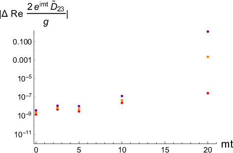
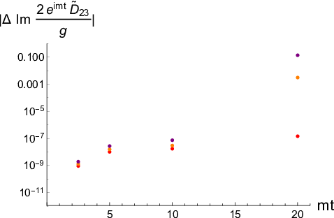
Refer to caption
(a) |Δ​ℜ⁡e​ei​m​t​D~23g/2||\Delta\Re e\,e^{imt}\frac{\tilde{D}_{23}}{g/2}|
Refer to caption
(b) |Δ​ℑ⁡m​ei​m​t​D~23g/2||\Delta\Im m\,e^{imt}\frac{\tilde{D}_{23}}{g/2}|
Figure 3: Modulus of differences between real and imaginary parts of ei​m​t​D~23g/2e^{imt}\frac{\tilde{D}_{23}}{g/2} for different system sizes at time instants m​t=0,2.5,5,10mt=0,2.5,5,10 and 2020 for a quench in the Ising model. The purple, orange, and red dots correspond to the difference of the value obtained for 30−4030-40, 40−5040-50 and 50−6050-60 in units of m​LmL.

These results demonstrate that terms growing with m​LmL indeed cancel.

J.2 Time dependence from Ci​n​t​B​I−I​IC^{intBI-II}

In this subsection we present numerical results to confirm that the time dependence of

g2​F1​e−i​m​t​∑I≠0|K⁡(ϑ1)|2​K​e​r​(ϑ1,t,R)ρ¯2​(ϑ1)​F5ε​(ϑ1)F1​Ω​(ϑ)+K′​(ϑ1)K⁡(ϑ1)−F5ε​(−ϑ1)F1​Ω​(ϑ)−K′​(−ϑ1)K⁡(−ϑ1)4sinhϑ1\frac{g}{2}F_{1}e^{-imt}\sum_{I\neq 0}\frac{|K(\vartheta_{1})|^{2}Ker(\vartheta_{1},t,R)}{\bar{\rho}_{2}(\vartheta_{1})}\frac{\frac{F_{5}^{\varepsilon}(\vartheta_{1})}{F_{1}\Omega(\vartheta)}+\frac{K^{\prime}(\vartheta_{1})}{K(\vartheta_{1})}-\frac{F_{5}^{\varepsilon}(-\vartheta_{1})}{F_{1}\Omega(\vartheta)}-\frac{K^{\prime}(-\vartheta_{1})}{K(-\vartheta_{1})}}{4\sinh\vartheta_{1}} (J.3)

in the term Ci​n​t​B​I−I​IC^{intBI-II} defined in (H.31), (I.2) is of the form

g2​F1​e−i​m​t​(Υ1​m​t+i​Υ2​log⁡m​t),\frac{g}{2}F_{1}e^{-imt}\left(\Upsilon_{1}mt+i\Upsilon_{2}\log mt\right)\;, (J.4)

and that

Υ1​m​t=∫−∞∞d​ϑ2​π​(|K⁡(ϑ)|2​ℜ⁡e​K​e​rs​t​a​c​(ϑ,t,R)​ℜ⁡e⁡(F5ε​(ϑ)F1​Ω​(ϑ)+K′​(ϑ)K⁡(ϑ1)−F5ε​(−ϑ)F1​Ω​(ϑ)−K′​(−ϑ)K⁡(−ϑ))​tanh⁡ϑ)′4​sinh⁡ϑ.\Upsilon_{1}mt=\int_{-\infty}^{\infty}\frac{d\vartheta}{2\pi}\frac{\left(|K(\vartheta)|^{2}\Re e\,Ker_{stac}(\vartheta,t,R)\,\Re e\,\left(\frac{F_{5}^{\varepsilon}(\vartheta)}{F_{1}\Omega(\vartheta)}+\frac{K^{\prime}(\vartheta)}{K(\vartheta_{1})}-\frac{F_{5}^{\varepsilon}(-\vartheta)}{F_{1}\Omega(\vartheta)}-\frac{K^{\prime}(-\vartheta)}{K(-\vartheta)}\right)\tanh\vartheta\right)^{\prime}}{4\sinh\vartheta}\;. (J.5)

For the numerical analysis we used the Ising model to demonstrate these statements with

K⁡(ϑ)=−i​g22​sinh⁡ϑ,K(\vartheta)=-i\frac{g^{2}}{2\sinh\vartheta}\;, (J.6)

where F5ε​(ϑ)=8​F1sinh⁡ϑF_{5}^{\varepsilon}(\vartheta)=\frac{8F_{1}}{\sinh\vartheta}, yielding

g2​F1​e−i​m​t​∑I≠0|K⁡(ϑ1)|2​(2−cosh⁡ϑ1)​K​e​r​(ϑ1,t,R)ρ¯2​(ϑ1)​2​sinh2⁡ϑ1\frac{g}{2}F_{1}e^{-imt}\sum_{I\neq 0}\frac{|K(\vartheta_{1})|^{2}\left(2-\cosh\vartheta_{1}\right)Ker(\vartheta_{1},t,R)}{\bar{\rho}_{2}(\vartheta_{1})2\sinh^{2}\vartheta_{1}} (J.7)

and

Υ1​m​t=∫−∞∞d​ϑ2​π​(|K⁡(ϑ)|2​(2−cosh⁡ϑ1)/cosh⁡ϑ​ℜ⁡e​K​e​rs​t​a​c​(ϑ,t,R))′2​sinh⁡ϑ.\Upsilon_{1}mt=\int_{-\infty}^{\infty}\frac{d\vartheta}{2\pi}\frac{\left(|K(\vartheta)|^{2}\left(2-\cosh\vartheta_{1}\right)/\cosh\vartheta\,\Re e\,Ker_{stac}(\vartheta,t,R)\right)^{\prime}}{2\sinh\vartheta}\;. (J.8)

Figure 4 shows the numerical results for (J.7) for system sizes m​L=50,60mL=50,60 and for various time instants. The kernel K​e​rKer was determined by numerical integration and we subtracted the m​LmL residue term

g2​F1​e−i​m​t​g44​m​L​K​e​r​(ϑ,t,0)′′8,\frac{g}{2}F_{1}e^{-imt}\frac{g^{4}}{4}\frac{mLKer(\vartheta,t,0)^{\prime\prime}}{8}\;, (J.9)

from (I.20) to check the resulted m​LmL independence.

Refer to caption
(a) ℜ⁡e​ei​m​t​Ci​n​t​B​I−I​IF1​g/2−m​L​K​e​r′′​g432\Re e\,e^{imt}\frac{C^{intBI-II}}{F_{1}g/2}-mL\frac{Ker^{\prime\prime}g^{4}}{32}
Refer to caption
(b) ℑ⁡m​ei​m​t​Ci​n​t​B​I−I​IF1​g/2−m​L​K​e​r′′​g432\Im m\,e^{imt}\frac{C^{intBI-II}}{F_{1}g/2}-mL\frac{Ker^{\prime\prime}g^{4}}{32}
Figure 4: Real and imaginary parts of ei​m​t​Ci​n​t​B​I−I​IF1​g/2−m​L​K​e​r′′​g432e^{imt}\frac{C^{intBI-II}}{F_{1}g/2}-mL\frac{Ker^{\prime\prime}g^{4}}{32} calculated with a discrete sum for time instants m​t=0.1,1,2.5,5,7.5,10,15,20,25,30,35mt=0.1,1,2.5,5,7.5,10,15,20,25,30,35 and 4040 for a quench in the Ising model. The orange and red symbols correspond to system sizes m​L=50mL=50 and 6060. g=1g=1.

Figure 5 shows the real and imaginary factor multiplying the term g2​F1​e−i​m​t\frac{g}{2}F_{1}e^{-imt} in Ci​n​t​B​I−I​IC^{intBI-II} calculated by a discrete summation (J.7) and by the integration (J.8). For the imaginary parts, we also keep the FS+FCF_{S}+F_{C} part from K​e​rs​t​a​cKer_{stac} (I.7) but drop the sinh2⁡ϑ\sqrt{\sinh^{2}\vartheta} type function, ff.

Refer to caption
(a) ℜ⁡e​ei​m​t​Ci​n​t​B​I−I​IF1​g/2−m​L​K​e​r′′​g432\Re e\,e^{imt}\frac{C^{intBI-II}}{F_{1}g/2}-mL\frac{Ker^{\prime\prime}g^{4}}{32}
Refer to caption
(b) ℑ⁡m​ei​m​t​Ci​n​t​B​I−I​IF1​g/2−m​L​K​e​r′′​g432\Im m\,e^{imt}\frac{C^{intBI-II}}{F_{1}g/2}-mL\frac{Ker^{\prime\prime}g^{4}}{32}
Figure 5: Real and imaginary parts of ei​m​t​Ci​n​t​B​I−I​IF1​g/2−m​L​K​e​r′′​g432e^{imt}\frac{C^{intBI-II}}{F_{1}g/2}-mL\frac{Ker^{\prime\prime}g^{4}}{32} calculated by a discrete sum and a continuous integral using K​e​rs​t​a​cKer_{stac} for time instants m​t=0.1,1,2.5,5,7.5,10,15,20,25,30,35mt=0.1,1,2.5,5,7.5,10,15,20,25,30,35 and 4040 for a quench in the Ising model. The red dots correspond to system sizes m​L=60mL=60 and the blue dots to the analytic results. g=1g=1.

We can conclude that for the real part multiplying g2​F1​e−i​m​t\frac{g}{2}F_{1}e^{-imt} using the real part of K​e​rs​t​a​cKer_{stac} in (J.8) gives a correct result. For the imaginary part, however, the imaginary part without the singular ff from K​e​rs​t​a​cKer_{stac} alone is not able to reproduce the result of the discrete summation. On the other hand, the time dependence of the imaginary coefficient is only logarithmic, and therefore the calculation of this sub-leading time dependence is not addressed in this work. We also checked if the linear time dependence can be described by

g44​1π​m​t,\frac{g^{4}}{4}\frac{1}{\pi}mt\;,

as predicted in Appendix I and if the logarithmic time dependence for the imaginary part is a correct assumption. In Fig. 6 we therefore fit the functions a+b​m​ta+b\,mt and a+b​ln⁡m​ta+b\,\ln mt to the real and imaginary parts of

ei​m​t​Ci​n​t​B​I−I​IF1​g/2−m​L​K​e​r′′​g432e^{imt}\frac{C^{intBI-II}}{F_{1}g/2}-mL\frac{Ker^{\prime\prime}g^{4}}{32}

calculated by the discrete summation with m​L=60mL=60 omitting the first 3 data points corresponding to the shortest times m​t=0.01,1,2.5mt=0.01,1,2.5.

Refer to caption
(a) ℜ⁡e​ei​m​t​Ci​n​t​B​I−I​IF1​g/2−m​L​K​e​r′′​g432\Re e\,e^{imt}\frac{C^{intBI-II}}{F_{1}g/2}-mL\frac{Ker^{\prime\prime}g^{4}}{32}
Refer to caption
(b) ℑ⁡m​ei​m​t​Ci​n​t​B​I−I​IF1​g/2−m​L​K​e​r′′​g432\Im m\,e^{imt}\frac{C^{intBI-II}}{F_{1}g/2}-mL\frac{Ker^{\prime\prime}g^{4}}{32}
Figure 6: Real and imaginary parts of ei​m​t​Ci​n​t​B​I−I​IF1​g/2−m​L​K​e​r′′​g432e^{imt}\frac{C^{intBI-II}}{F_{1}g/2}-mL\frac{Ker^{\prime\prime}g^{4}}{32} calculated by a discrete sum using K​e​rs​t​a​cKer_{stac} for various time instants for a quench in the Ising model. The red dots correspond to system sizes m​L=60mL=60 and the blue line to the fitted curves of type a+b​m​ta+b\,mt and a+b​ln⁡m​ta+b\,\ln mt.

From the linear regression, the coefficient of the linearly time-dependent term is 0.07991670.0799167 which is to be compared with 14​π=0.0795775\frac{1}{4\pi}=0.0795775 as g=1g=1. The agreement is excellent, and although the error of the fitted parameter is 7×10−57\times 10^{-5}, the match is convincing.

J.3 Comparing the time dependence of D~23\tilde{D}_{23} with the analytic results

In this subsection we study the time dependence of

ei​m​t​D~23g/2e^{imt}\frac{\tilde{D}_{23}}{g/2}

for the Ising model with K=−i​g2sinh⁡2​ϑK=-i\frac{g^{2}}{\sinh 2\vartheta} for m​L=70mL=70. We compute this quantity using discrete finite volume summation for various time instants, and fit its real and imaginary parts with the appropriate function dependences a+b​m​t+c​m​t+d​m​t​ln⁡m​ta+b\,\sqrt{mt}+c\,mt+d\,mt\ln mt and a+b​m​t+c​m​ta+b\,\sqrt{mt}+c\,mt dictated by our analysis done in Appendix I, omitting the first 7 data points corresponding to short times.

Refer to caption
(a) ℜ⁡e​ei​m​t​D~23g/2\Re e\,e^{imt}\frac{\tilde{D}_{23}}{g/2}
Refer to caption
(b) ℑ⁡m​ei​m​t​D~23g/2\Im m\,e^{imt}\frac{\tilde{D}_{23}}{g/2}
Figure 7: Real and imaginary parts of ei​m​t​D~23g/2e^{imt}\frac{\tilde{D}_{23}}{g/2} for time instants m​t=0,1,2​…,35mt=0,1,2...,35 for a quench in the Ising model. The red dots correspond to system sizes m​L=70mL=70 and the blue curve to to the fitted curves of type a+b​m​t+c​m​t+d​m​t​ln⁡m​ta+b\,\sqrt{mt}+c\,mt+d\,mt\ln mt and a+b​m​t+c​m​ta+b\,\sqrt{mt}+c\,mt. g=1g=1.

Concerning the real parts, the values obtained from the fit are d=−0.0825821d=-0.0825821 and c=0.149943c=0.149943, which must be compared with −14​π=−0.0795775-\frac{1}{4\pi}=-0.0795775 and 𝒦+34​π=0.131292\mathcal{K}+\frac{3}{4\pi}=0.131292 resulting from (3.30) and (3.31) with g=1g=1 and S=−1S=-1. The accuracy of the fit itself is around 10−3−10−410^{-3}-10^{-4}. The difference between the fitted parameters and the analytic predictions is now a bit larger compared to the previous subsection. However, neglecting more data points for short times the fitted values move towards the analytic predictions. We note however, that omitting too many points leads to a deterioration of the fit quality, as for an accurate determination of a logarithmic term data points over several orders of magnitude should be used, which is not possible to extract due to the inaccuracy of the discrete sum for large times. As an additional test we also tried the fitting function a+b​m​t+c​m​ta+b\,\sqrt{mt}+c\,mt and noted that the fit residuals were two orders of magnitude larger than for the case including the term m​t​ln⁡m​tmt\ln mt, which is a confirmation of the presence of the term m​t​ln⁡m​tmt\ln mt in the time dependence.

For the imaginary part the parameter cc was found to be c=0.114809c=0.114809 which must be compared with 18=0.125\frac{1}{8}=0.125 for g=1g=1 according to (3.30) and (3.31). The total estimated error of the fitted value is of the order 10−3.10^{-3}. In principle we should have either included ln⁡m​t\ln mt in the fitting function or subtracted the contribution of ℑ⁡m​ei​m​t​Ci​n​t​B​I−I​IF1​g/2−m​L​K​e​r′′​g432\Im m\,e^{imt}\frac{C^{intBI-II}}{F_{1}g/2}-mL\frac{Ker^{\prime\prime}g^{4}}{32} discussed in the previous subsection from the data points, but since this correction is rather small it was simply discarded.