An offline/online procedure for dual norm calculations of parameterized functionals: empirical quadrature and empirical test spaces

Abstract

We present an offline/online computational procedure for computing the dual norm of parameterized linear functionals. The approach is motivated by the need to efficiently compute residual dual norms, which are used in model reduction to estimate the error of a given reduced solution. The key elements of the approach are (i) an empirical test space for the manifold of Riesz elements associated with the parameterized functional, and (ii) an empirical quadrature procedure to efficiently deal with parametrically non-affine terms. We present a number of theoretical and numerical results to identify the different sources of error and to motivate the proposed technique, and we compare the approach with other state-of-the-art techniques. Finally, we investigate the effectiveness of our approach to reduce both offline and online costs associated with the computation of the time-averaged residual indicator proposed in [Fick, Maday, Patera, Taddei, Journal of Computational Physics, 2018].

Tommaso Taddei¹

¹ Institut de Mathématiques de Bordeaux, Team MEMPHIS, INRIA Bordeaux - Sud Ouest tommaso.taddei@inria.fr

Keywords: Reduced basis method, hyper-reduction, dual norm estimation.

1 Introduction

A posteriori error estimators are designed to assess the accuracy of a given numerical solution in a proper metric of interest. In the context of Model Order Reduction (MOR, [29, 23]), a posteriori error estimators are employed during the offline stage to drive the construction of the Reduced Order Model (ROM), and also during the online stage to certify the accuracy of the estimate. The vast majority of error estimators employed in MOR procedures relies on the evaluation of the dual norm of the residual: for nonlinear and non-parametrically affine problems, this task might be particularly demanding both in terms of memory requirements and of computational cost. Motivated by these considerations, the objective of this paper is to develop and analyze an offline/online computational strategy for the computation of the dual norm of parameterized functionals.

Given the parameter space $\mathcal{P}\subset\mathbb{R}^{P}$ and the domain $\Omega\subset\mathbb{R}^{d}$ , we introduce the Hilbert space $\mathcal{X}$ defined over $\Omega$ endowed with the inner product $(\cdot,\cdot)_{\mathcal{X}}$ and the induced norm $\|\cdot\|_{\mathcal{X}}:=\sqrt{(\cdot,\cdot)_{\mathcal{X}}}$ . We denote by $\mathcal{X}^{\prime}$ the dual space of $\mathcal{X}$ , and we define the Riesz operator $R_{\mathcal{X}}:\mathcal{X}^{\prime}\to\mathcal{X}$ such that $(R_{\mathcal{X}}\mathcal{L},\,v)_{\mathcal{X}}=\mathcal{L}(v)$ for all $v\in\mathcal{X}$ and $\mathcal{L}\in\mathcal{X}^{\prime}$ . Exploiting these definitions, our goal is to reduce the marginal (i.e., in the limit of many queries) cost associated with the computation of the dual norm of the parameterized functional $\mathcal{L}_{\mu}$ ,

\|\mathcal{L}_{\mu}\|_{\mathcal{X}^{\prime}}:=\sup_{v\in\mathcal{X}}\,\frac{\mathcal{L}_{\mu}(v)}{\|v\|_{\mathcal{X}}}=\|R_{\mathcal{X}}\mathcal{L}_{\mu}\|_{\mathcal{X}},

(1)

for $\mu\in\mathcal{P}$ . We are interested in functionals of the form

\mathcal{L}_{\mu}(v)=\int_{\Omega}\,\eta(x;v,\mu)\,dx,\hskip 10.00002pt\eta(x;v,\mu)=\Upsilon_{\mu}(x)\cdot F(x;v),

(2)

where $\Upsilon:\Omega\times\mathcal{P}\to\mathbb{R}^{D}$ is a given function of spatial coordinate and parameter, and $F$ is a linear function of $v$ and possibly its derivatives. Throughout the work, we shall consider $H_{0}^{1}(\Omega)\subset\mathcal{X}\subset H^{1}(\Omega)$ , and $F(x;v)=[v(x),\nabla v(x)]$ . However, our discussion can be extended to other classes of functionals and other choices of the ambient space $\mathcal{X}$ .

If $\mathcal{L}_{\mu}$ is parametrically-affine, i.e. $\mathcal{L}_{\mu}(v)=\sum_{m=1}^{M}\,\Theta_{m}(\mu)\mathcal{L}_{m}(v)$ with $M=\mathcal{O}(1)$ , then computations of $\|\mathcal{L}_{\mu}\|_{\mathcal{X}^{\prime}}$ can be performed efficiently exploiting the linearity of the Riesz operator; on the other hand, if $\mathcal{L}_{\mu}$ is not parametrically-affine, hyper-reduction techniques should be employed. Over the past decade, many authors have proposed hyper-reduction procedures for the efficient evaluation of parameterized integrals: these techniques can be classified as Approximation-Then-Integration (ATI) approaches or Empirical Quadrature (EQ) approaches. ATI approaches (i) construct a suitable reduced basis and an associated interpolation/approximation system for $\Upsilon_{\mu}$ in (2), and then (ii) precompute all required integrals during an offline stage. Conversely, EQ procedures — also known as Reduced-Order Quadrature procedures ([2]) — directly approximate the integrals in (2) by developing a specialized low-dimensional empirical quadrature rule. Representative ATI approaches for model reduction applications are Gappy-POD, which was first proposed in [18] for image reconstruction and then adapted to MOR in [11, 12, 3], and the Empirical Interpolation Method (EIM, [5, 21]) and related approaches ([17, 27, 14, 31, 15]). On the other hand, EQ approaches have been proposed in [1, 2, 19, 28].

As explained in [28], although ATI approaches are quite effective in practice, the objective of function approximation and integration are arguably quite different and it is thus difficult to relate the error in integrand approximation to the error in dual norm prediction. As a result, rather conservative selections of the approximation tolerance are required in practice to ensure that the dual norm estimate is sufficiently accurate. On the other hand, since the test space in (1) is infinite-dimensional, EQ approaches cannot be applied as is, unless the Riesz element $\xi_{\mu}:=R_{\mathcal{X}}\,\mathcal{L}_{\mu}$ is known explicitly.

We here propose an offline/online procedure that relies on two key ingredients: empirical test spaces, and empirical quadrature. We resort to Proper Orthogonal Decomposition (POD, [6, 32, 35]) to generate a $J_{\rm es}$ -dimensional reduced space $\mathcal{X}_{J_{\rm es}}$ that approximates the manifold of Riesz elements associated with $\mathcal{L}$ , $\mathcal{M}_{\mathcal{L}}=\{R_{\mathcal{X}}\mathcal{L}_{\mu}:\;\;\mu\in\mathcal{P}\}$ . Then, we approximate the dual norm $\|\mathcal{L}_{\mu}\|_{\mathcal{X}^{\prime}}$ using $\|\mathcal{L}_{\mu}\|_{\mathcal{X}_{J_{\rm es}}^{\prime}}$ . Estimation of $\|\mathcal{L}_{\mu}\|_{\mathcal{X}_{J_{\rm es}}^{\prime}}$ involves the approximation of $J_{\rm es}$ integrals: we might thus rely on empirical quadrature procedures to estimate the latter dual norm.

The contributions of the present work are threefold: (i) an actionable procedure for the construction of empirical test spaces; (ii) the reinterpretation of the EQ problem as a sparse representation problem and the application of EQ to dual norm estimation; and (iii) a thorough numerical and also theoretical investigation of the performance of several ATI and EQ+ES hyper-reduction techniques for dual norm prediction.

(i)

Empirical test spaces are closely related to $\ell_{2}$ -embeddings, which have been recently proposed for MOR applications by Balabanov and Nouy in [4]. In section 2.2, we formally link empirical test spaces for dual norm calculations to $\ell_{2}$ -embeddings, and we discuss the differences in their practical constructions. Furthermore, in section 2.5, we present an a priori error bound that motivates our construction.
(ii)

The problem of sparse representation — or equivalently best subset selection — has been widely studied in the optimization, statistics and signal processing literature, and several solution strategies are available, including $\ell^{1}$ relaxation [16], Greedy algorithms [34], and more recently mixed integer optimization procedures [7]. In this work, we show that the problem of EQ can be recast as a sparse representation problem, and we consider three different approaches based on $\ell^{1}$ minimization (here referred to as $\ell^{1}$ -EQ), on the EIM greedy algorithm (EIM-EQ), and on Mixed Integer Optimization (MIO-EQ), respectively. We remark that $\ell^{1}$ -EQ has been first proposed in [28] for empirical quadrature, while EIM-EQ has been first proposed in [2]; on the other hand, MIO-EQ is new in this context. In order to reduce the cost associated with the construction of the quadrature rule, we further propose a divide-and-conquer strategy to reduce the dimension of the optimization problem to be solved offline.
(iii)

To our knowledge, a detailed comparison of ATI approaches and EQ approaches for hyper-reduction is currently missing in the literature. In sections 3 and 4 we present numerical and also theoretical results that offer insights about the potential benefits and drawbacks of ATI and EQ techniques, in the context of dual norm prediction.

The paper is organized as follows. In section 2, we present the computational procedure, and we prove an a priori error bound that relates the prediction error in dual norm estimation to the quadrature error and to the discretization error associated with the introduction of the empirical test space. In section 3, we review ATI approaches for dual norm calculations and we offer several remarks concerning the benefits and the drawbacks of the proposed strategies. Furthermore, in section 4, we present numerical results to compare the performance of our EQ+ES method for the three EQ procedures considered with a representative ATI approach; in particular, we apply the proposed technique to the computation of the dual time-averaged residual presented in [20], associated with the Reduced Basis approximation of the solution to a 2D unsteady incompressible Navier-Stokes problem. Finally, in section 5, we summarize the key contributions and identify several future research directions.

2 Methodology

2.1 Formulation

In view of the presentation of the methodology, we introduce the high-fidelity (truth) space $\mathcal{X}_{\rm hf}={\rm span}\{\varphi_{i}\}_{i=1}^{\mathcal{N}}\subset\mathcal{X}$ and the high-fidelity quadrature rule

\mathcal{Q}^{\rm hf}(v):=\sum_{i=1}^{\mathcal{N}_{\rm q}}\,\rho_{i}^{\rm hf}\,v(x_{i}^{\rm hf}).

We endow $\mathcal{X}_{\rm hf}$ with the inner product $(w,v)_{\mathcal{X}_{\rm hf}}=\mathcal{Q}^{\rm hf}(\lambda(\cdot;w,v))$ for a suitable choice¹¹ 1 In all our examples, we consider $\lambda(\cdot;w,v)=\nabla w\cdot\nabla v+u\,v$ . of $\lambda$ , and we approximate the functional in (2) as $\mathcal{L}_{\mu,\rm hf}(v):=\mathcal{Q}^{\rm hf}(\eta(\cdot;v,\mu))$ . In the remainder, we shall assume that $\|\mathcal{L}_{\mu,\rm hf}\|_{\mathcal{X}_{\rm hf}^{\prime}}\approx\|\mathcal{L}_{\mu}\|_{\mathcal{X}^{\prime}}$ for all $\mu\in\mathcal{P}$ . Since our approach builds upon the high-fidelity discretization, in the following we exclusively deal with high-fidelity quantities: to simplify notation, we omit the subscript $(\cdot)_{\rm hf}$ .

Given $v\in\mathcal{X}$ , we denote by $\mathbf{v}\in\mathbb{R}^{\mathcal{N}}$ the corresponding vector of coefficients, $v(x)=\sum_{i=1}^{\mathcal{N}}\,{v}_{i}\,\varphi_{i}(x)$ ; similarly, given $\mathcal{L}\in\mathcal{X}^{\prime}$ , we define $\boldsymbol{\mathcal{L}}\in\mathbb{R}^{\mathcal{N}}$ such that $\left(\boldsymbol{\mathcal{L}}\right)_{i}=\mathcal{L}(\varphi_{i})$ . By straightforward calculations, we find the following expression for the dual norm:

L(\mu):=\|\mathcal{L}_{\mu}\|_{\mathcal{X}^{\prime}}=\sup_{v\in\mathcal{X}}\,\frac{\mathcal{Q}^{\rm hf}(\eta(\cdot;v,\mu))}{\|v\|_{\mathcal{X}}}\,=\,\sqrt{\boldsymbol{\mathcal{L}}_{\mu}^{T}\,\mathbb{X}^{-1}\boldsymbol{\mathcal{L}}_{\mu}},

(3)

where $\mathbb{X}_{i,j}=(\varphi_{j},\varphi_{i})_{\mathcal{X}}$ . Evaluation of $L$ in (3) for a given $\mu\in\mathcal{P}$ requires the solution to a linear system of size $\mathcal{N}$ , which costs $C_{\rm riesz}=\mathcal{O}(\mathcal{N}^{s})$ for some $s\in[1,2)$ .

To reduce the costs, we propose to substitute $\mathcal{X}$ in (3) with the $J_{\rm es}$ -dimensional empirical test space $\mathcal{X}_{J_{\rm es}}={\rm span}\{\phi_{j}\}_{j=1}^{J_{\rm es}}$ where $(\phi_{j},\phi_{i})_{\mathcal{X}}=\delta_{i,j}$ , and the high-fidelity quadrature rule $\mathcal{Q}^{\rm hf}$ with the $Q_{\rm eq}$ -dimensional quadrature rule

\mathcal{Q}^{\rm eq}(v)\,=\,\sum_{q=1}^{Q_{\rm eq}}\,\rho_{q}^{\rm eq}\,v(x_{q}^{\rm eq}),\hskip 10.00002pt{\rm for\,some}\;\{\rho_{q}^{\rm eq},x_{q}^{\rm eq}\}_{q=1}^{Q_{\rm eq}}\subset\mathbb{R}\times\Omega.

Exploiting the fact that $\{\phi_{j}\}_{j}$ is an orthonormal basis of $\mathcal{X}_{J_{\rm es}}$ , we obtain the EQ+ES estimate of $L(\mu)$ :

	$\begin{array}[]{rl}\displaystyle{L_{J_{\rm es},Q_{\rm eq}}(\mu)\,=}&\displaystyle{\sup_{v\in\mathcal{X}_{J_{\rm es}}}\,\frac{\mathcal{Q}^{\rm eq}(\eta(\cdot;v,\mu))}{\\|v\\|_{\mathcal{X}}}\,=\,\sqrt{\sum_{j=1}^{J_{\rm es}}\,\left(\mathcal{Q}^{\rm eq}(\eta(\cdot;\phi_{j},\mu)\right)^{2}}}\\[8.53581pt] =&\displaystyle{\\|\mathbb{H}(\mu)\boldsymbol{\rho}^{\rm eq}\\|_{2},}\end{array}$	(4a)
where
	$\left(\mathbb{H}(\mu)\right)_{q,j}\,=\,\eta(x_{q}^{\rm eq};\phi_{j},\mu)\,=\,\sum_{i=1}^{D}\,\left(\Upsilon_{\mu}(x_{q}^{\rm eq})\right)_{i}\,\left(F(x_{q}^{\rm eq};v)\right)_{i}.$	(4b)

It is straightforward to verify that, if $\eta$ is of the form (2), computation of the matrix $\mathbb{H}(\mu)$ scales with $\mathcal{O}(D\,J_{\rm es}\,Q_{\rm eq})$ : provided that $J_{\rm es},\,Q_{\rm eq}\ll\mathcal{N}$ , evaluation of (4) is thus significantly less expensive than the evaluation of (3).

Below, we discuss how to practically build the space $\mathcal{X}_{J_{\rm es}}$ (section 2.2), and the quadrature rule $\mathcal{Q}^{\rm eq}(\cdot)$ (section 2.3). Then, in section 2.4, we briefly summarize the overall procedure and we comment on offline and online costs. Finally, in section 2.5, we present an a priori error bound that shows that the prediction error is the sum of two contributions: a quadrature error, and a discretization error associated with the empirical test space.

Remark 2.1.

EQ estimate of $\mathbf{L}(\boldsymbol{\mu})$ . The EQ estimate of $L(\mu)$ ,

L_{Q_{\rm eq}}(\mu)=\sup_{v\in\mathcal{X}}\,\frac{\mathcal{Q}^{\rm eq}(\eta(\cdot;v,\mu))}{\|v\|_{\mathcal{X}}},

is not in general related to $L(\mu)$ for $Q_{\rm eq}<\mathcal{N}_{\rm q}$ . For this reason, EQ approaches cannot be applied as is to estimate $L(\mu)$ .

2.2 Empirical test space

Recalling the Riesz representation theorem, we find that $L({\mu})^{2}=\mathcal{L}_{\mu}\left(\xi_{\mu}\right),$ for all $\mu\in\mathcal{P}$ , $\xi_{\mu}=R_{\mathcal{X}}\,\mathcal{L}_{\mu}$ ; therefore, if $\mathcal{X}_{J_{\rm es}}$ accurately approximates the elements of the manifold $\mathcal{M}_{\mathcal{L}}\,=\,\left\{\xi_{\mu}:\;\mu\in\mathcal{P}\right\}$ , we expect that

L(\mu)=\sup_{v\in\mathcal{M}_{\mathcal{L}}}\,\frac{\mathcal{L}_{\mu}(v)}{\|v\|_{\mathcal{X}}}\,\approx\,\sup_{v\in\mathcal{X}_{J_{\rm es}}}\,\frac{\mathcal{L}_{\mu}(v)}{\|v\|_{\mathcal{X}}}=:\|\mathcal{L}_{\mu}\|_{\mathcal{X}_{J_{\rm es}}^{\prime}}.

(5)

We provide a rigorous justification of this approximation in section 2.5.

We construct the approximation space $\mathcal{X}_{J_{\rm es}}$ using POD. First, we generate the training set $\Xi^{\rm train,es}=\{\mu^{\ell}\}_{\ell=1}^{n_{\rm train}^{\rm es}}\subset\mathcal{P}$ , where $\mu^{1},\ldots,\mu^{n_{\rm train}^{\rm es}}\overset{\rm iid}{\sim}{\rm Uniform}(\mathcal{P})$ ; then we compute $\xi^{\ell}=\xi_{\mu^{\ell}}$ for $\ell=1,\ldots,n_{\rm train}^{\rm es}$ ; finally, we use the snapshots $\{\xi^{\ell}\}_{\ell=1}^{n_{\rm train}^{\rm es}}$ to compute the POD space $\mathcal{X}_{J_{\rm es}}$ (see [32]) based on the $\mathcal{X}$ -inner product.

Remark 2.2.

Choice of $n_{\rm train}^{\rm es}$ and ${J_{\rm es}}$ . In order to validate the choice of $n_{\rm train}^{\rm es}$ and ${J_{\rm es}}$ , we might introduce $n_{\rm test}^{\rm es}$ additional samples $\tilde{\mu}^{1},\ldots,\tilde{\mu}^{n_{\rm test}^{\rm es}}\sim{\rm Uniform}(\mathcal{P})$ , and compute the error indicators²² 2 We observe that $E_{{J_{\rm es}},n_{\rm train}^{\rm es},n_{\rm test}^{\rm es}}^{(\infty)}$ is equivalent to the error indicator proposed in [10].

E_{{J_{\rm es}},n_{\rm train}^{\rm es},n_{\rm test}^{\rm es}}^{(\infty)}=\max_{k=1,\ldots,n_{\rm test}^{\rm es}}\,\|\Pi_{\mathcal{X}_{J_{\rm es}}^{\perp}}\,\xi_{\tilde{\mu}^{k}}\|_{\mathcal{X}},

(6)

and

E_{{J_{\rm es}},n_{\rm train}^{\rm es},n_{\rm test}^{\rm es}}^{(2)}=\frac{1}{n_{\rm test}^{\rm es}}\,\sum_{k=1}^{n_{\rm test}^{\rm es}}\,\|\Pi_{\mathcal{X}_{J_{\rm es}}^{\perp}}\,\xi_{\tilde{\mu}^{k}}\|_{\mathcal{X}}^{2},

(7)

where $\mathcal{X}_{J_{\rm es}}^{\perp}$ denotes the orthogonal complement of $\mathcal{X}_{J_{\rm es}}$ , and $\Pi_{\mathcal{X}_{J_{\rm es}}^{\perp}}:\mathcal{X}\to{\mathcal{X}_{J_{\rm es}}^{\perp}}$ is the orthogonal projection operator. $E_{{J_{\rm es}},n_{\rm train}^{\rm es},n_{\rm test}^{\rm es}}^{(\infty)}$ provides an estimate of the discretization error that enters in the a priori error bound in Proposition 2.2, while $E_{{J_{\rm es}},n_{\rm train}^{\rm es},n_{\rm test}^{\rm es}}^{(2)}$ can be compared with the in-sample error $E_{{J_{\rm es}},n_{\rm train}^{\rm es}}^{(2)}=\frac{1}{n_{\rm train}^{\rm es}}\,\sum_{\ell=1}^{n_{\rm train}^{\rm es}}\,\|\Pi_{\mathcal{X}_{J_{\rm es}}^{\perp}}\,\xi_{\mu^{\ell}}\|_{\mathcal{X}}^{2}$ to assess the representativity of the training set $\Xi^{\rm train,es}$ .

Connection with $\ell_{2}$ -embeddings

Exploiting notation introduced in section 2.1, and recalling that $\{\phi_{j}\}_{j}$ is an orthonormal basis of $\mathcal{X}_{J_{\rm es}}$ , we can rewrite (5) as follows:

\|\mathcal{L}_{\mu}\|_{\mathcal{X}_{J_{\rm es}}^{\prime}}=\|\mathbb{X}_{J_{\rm es}}^{T}\boldsymbol{\mathcal{L}}_{\mu}\|_{2},

(8)

where $\mathbb{X}_{J_{\rm es}}=[\boldsymbol{\phi}_{1},\ldots,\boldsymbol{\phi}_{J_{\rm es}}]$ . In [4] (see [4, section 3.1]), the authors propose to estimate $L(\mu)$ as

L_{\Theta}(\mu)=\|\Theta\mathbb{X}^{-1}\boldsymbol{\mathcal{L}}_{\mu}\|_{2},

(9)

where $\Theta\in\mathbb{R}^{J_{\rm es}\times\mathcal{N}}$ is called $\mathcal{X}\to\ell_{2}$ embedding. By comparing (8) with (9), we deduce that the approach proposed here corresponds to that in [4], provided that $\Theta=\mathbb{X}_{J_{\rm es}}^{T}\mathbb{X}$ .

The key difference between the two approaches is in the practical construction of $\Theta$ . In [4], the authors consider $\Theta=\boldsymbol{\Omega}\mathbb{Q}$ where $\mathbb{Q}\in\mathbb{R}^{\mathcal{N}\times\mathcal{N}}$ is the upper-triangular matrix associated with the Cholesky factorization of $\mathbb{X}$ , while $\boldsymbol{\Omega}\in\mathbb{R}^{J_{\rm es}\times\mathcal{N}}$ is the realization of a random matrix — distributed according to the rescaled Gaussian distribution, the rescaled Rademacher distribution, or the partial subsampled randomized Hadamard transform (P-SRHT). For these three choices of the sampling distribution, the authors prove a priori error bounds in probability, which provide estimates for the minimum value of $J_{\rm es}$ required to achieve a target accuracy.

Recalling the optimality of POD (see, e.g., [35]), for sufficiently large values of $n_{\rm train}^{\rm es}$ , we expect that our approach leads to smaller test spaces — and thus more efficient online calculations for any target accuracy. On the other hand, the construction of $\Theta$ in [4] requires significantly less offline resources than the construction of $\mathcal{X}_{J_{\rm es}}$ . For this reason, the choice between the two approaches is extremely problem- and architecture-dependent.

2.3 Empirical quadrature

We shall now address the problem of determining the quadrature rule

\mathcal{Q}^{\rm eq}(v)\,=\,\sum_{q=1}^{Q_{\rm eq}}\,\rho_{q}^{\rm eq}\,v(x_{q}^{\rm eq})

in (4). Towards this end, we assume that $\{x_{q}^{\rm eq}\}_{q}\subset\{x_{i}^{\rm hf}\}_{i}$ ; then, we define the quadrature rule operator $\mathcal{Q}:C(\Omega)\times\mathbb{R}^{\mathcal{N}_{\rm q}}\to\mathbb{R}$ such that

\mathcal{Q}(v,\boldsymbol{\rho})\,=\,\sum_{i=1}^{\mathcal{N}_{\rm q}}\,\rho_{i}\,v(x_{i}^{\rm hf}).

Exploiting the latter definition, we formulate the problem of finding $\{\rho_{q}^{\rm eq},x_{q}^{\rm eq}\}_{q}$ as the problem of finding $\boldsymbol{\rho}^{\star}\in\mathbb{R}^{\mathcal{N}_{\rm q}}$ such that

1.

the number of nonzero entries in $\boldsymbol{\rho}^{\star}$ is as small as possible;

the corresponding quadrature rule $\mathcal{Q}^{\star}(\cdot):=\mathcal{Q}(\cdot,\boldsymbol{\rho}^{\star})$ satisfies

\big|\mathcal{Q}^{\star}(\eta(\cdot;\phi_{j},\mu))\,-\,\mathcal{Q}^{\rm hf}(\eta(\cdot;\phi_{j},\mu))\big|\leq\delta,\hskip 20.00003ptj=1,\ldots,J_{\rm es},

(10)

for all $\mu$ in the training set $\Xi^{\rm train,eq}=\{\mu^{\ell}\}_{\ell=1}^{n_{\rm train}^{\rm eq}}$ , and

\big|\mathcal{Q}^{\star}(1)\,-\,\mathcal{Q}^{\rm hf}(1)\big|\leq\delta.

(11)

Given a (approximate) solution $\boldsymbol{\rho}^{\star}$ , we then extract the strictly non-null quadrature weights $\{\rho_{q}^{\rm eq},x_{q}^{\rm eq}\}_{q=1}^{Q_{\rm eq}}=\{\{\rho_{i}^{\star},x_{i}^{\rm hf}\}_{i}:\,i\in\{k:\rho_{k}^{\star}\neq 0\}\}$ .

The first requirement corresponds to minimizing the number of non-null weights $Q_{\rm eq}$ : recalling (4), minimizing $Q_{\rm eq}$ is equivalent to minimizing the online costs for a given choice of the empirical test space. Condition (10) controls the accuracy of the dual norm estimate, as discussed in the error analysis. On the other hand, as explained in [38], condition (11) is empirically found to improve the accuracy of the EQ procedure when the integral is close to zero due to the cancellation of the integrand in different parts of the domain. Finally, we remark that in [28, 38] the authors propose to add the non-negativity constraint

\rho_{i}^{\star}\geq 0,\hskip 10.00002pti=1,\ldots,\mathcal{N}_{\rm q}.

(12)

As discussed later in this section, the non-negativity constraint reduces by half the size of the problem that is practically solved during the offline stage for two of the EQ methods ( $\ell^{1}$ -EQ and MIO-EQ) employed in this work; furthermore, we observe that the non-negativity of the weights is used in [37] to prove a stability result for a Galerkin ROM. We here consider both the case of non-negative weights and the case of real-valued weights. We anticipate that for the latter case we are able to prove a theoretical result that motivates the approach.

These desiderata can be translated in the following minimization statement:

	$\min_{\boldsymbol{\rho}\in\mathbb{R}^{\mathcal{N}_{\rm q}}}\,\\|\boldsymbol{\rho}\\|_{0},\hskip 10.00002pt{\rm s.t.}\;\\|{\mathbb{G}}\boldsymbol{\rho}-{\mathbf{y}}^{\rm hf}\\|_{\infty}\leq\delta$	(13a)
where $\\|\cdot\\|_{\infty}$ denotes the $\infty$ norm, $\\|\mathbf{v}\\|_{\infty}=\max_{k}\|v_{k}\|$ , $\\|\cdot\\|_{0}$ denotes the $\ell^{0}$ “norm”³³ 3 $\\|\cdot\\|_{0}$ is not a norm since it does not satisfy the homogeneity property; nevertheless, it is called norm in the vast majority of the statistics and optimization literature. $\\|\boldsymbol{\rho}\\|_{0}=\#\{\rho_{i}\neq 0:\,i=1,\ldots,\mathcal{N}_{\rm q}\}$ , and $\mathbb{G}\in\mathbb{R}^{K\times\mathcal{N}_{\rm q}}$ and $\mathbf{y}^{\rm hf}\in\mathbb{R}^{K}$ , $K=n_{\rm train}^{\rm eq}J_{\rm es}+1$ , are defined as
	$\mathbb{G}=\left[\begin{array}[]{ccc}\eta(x_{1}^{\rm hf};\phi_{1},\mu^{1}),&\ldots&\eta(x_{\mathcal{N}_{\rm q}}^{\rm hf};\phi_{1},\mu^{1})\\ &\vdots&\\ \eta(x_{1}^{\rm hf};\phi_{J_{\rm es}},\mu^{n_{\rm train}^{\rm eq}}),&\ldots&\eta(x_{\mathcal{N}_{\rm q}}^{\rm hf};\phi_{J_{\rm es}},\mu^{n_{\rm train}^{\rm eq}})\\[5.69054pt] 1&\ldots&1\\ \end{array}\right],$	(13b)
	$\mathbf{y}^{\rm hf}=\left[\mathcal{Q}^{\rm hf}\left(\eta(\cdot;\phi_{1},\mu^{1})\right),\ldots\,,\,\mathcal{Q}^{\rm hf}\left(\eta(\cdot;\phi_{J_{\rm es}},\mu^{n_{\rm train}^{\rm eq}})\right),\mathcal{Q}^{\rm hf}\left(1\right)\right]$	(13c)

Alternatively, if we choose to include the non-negativity constraint, we obtain

\min_{\boldsymbol{\rho}\in\mathbb{R}^{\mathcal{N}_{\rm q}}}\,\|\boldsymbol{\rho}\|_{0},\hskip 10.00002pt{\rm s.t.}\;\left\{\begin{array}[]{l}\displaystyle{\|{\mathbb{G}}\boldsymbol{\rho}-{\mathbf{y}}^{\rm hf}\|_{\infty}\leq\delta}\\[5.69054pt] \boldsymbol{\rho}\geq\mathbf{0}\\ \end{array}\right.

(14)

Problems (13) and (14) can be interpreted as sparse representation problems where the input data — the high-fidelity integrals $\mathbf{y}^{\rm hf}$ — are noise-free. We emphasize that there are important differences between the two problems considered here and the sparse representation problems typically considered in the statistics literature, particularly in compressed sensing (CS, [16]). CS relies on the assumption that the original signal is sparse, and that the coherence among different columns of $\mathbb{G}$ is small (see, e.g., [9] for a thorough discussion). In our setting, these conditions are not expected to hold due to the smoothness in space of the elements of the manifold and to the deterministic nature of the problem. As a result, techniques developed and analyzed in the CS literature might be highly suboptimal in our context. After the seminal work by Bertsimas et al. [7], Hastie et al. [22] presented detailed empirical comparisons for several state-of-the-art approaches for datasets characterized by a wide spectrum of Signal-to-Noise Ratios.

As stated in the introduction, we here resort to three EQ approaches to approximate (13) and (14). While $\ell^{1}$ -EQ and EIM-EQ have been first presented in [28] and [2], MIO-EQ is new in this context. In the next three sections, we briefly illustrate the three EQ techniques.

Remark 2.3.

Dependence on the basis $\{\phi_{j}\}_{j}$ . Conditions (10) depend on the choice of the basis of $\mathcal{X}_{J_{\rm es}}$ . In particular, given $\tilde{\phi}=\sum_{j=1}^{J_{\rm es}}a_{j}\phi_{j}$ , if we define ${\eta}^{j,\ell}=\eta(\cdot;{\phi}_{j},\mu^{\ell})$ , we obtain

\begin{array}[]{l}\displaystyle{\big|\mathcal{Q}\left(\eta(\cdot;\tilde{\phi},\mu^{\ell});\boldsymbol{\rho}^{\star}\right)\,-\,\mathcal{Q}^{\rm hf}\left(\eta(\cdot;\tilde{\phi},\mu^{\ell})\right)\big|=\big|\sum_{j=1}^{J_{\rm es}}\,\left(\mathcal{Q}\left({\eta}^{j,\ell};\boldsymbol{\rho}^{\star}\right)\,-\,\mathcal{Q}^{\rm hf}\left({\eta}^{j,\ell}\right)\right)\,a_{j}\big|}\\[8.53581pt] \displaystyle{\leq\delta\|\mathbf{a}\|_{1}\leq\delta\|\mathbf{1}\|_{2}\|\mathbf{a}\|_{2}=\delta\sqrt{J_{\rm es}}\|\tilde{\phi}\|_{\mathcal{X}}}\\ \end{array}

Note that in the first inequality we used (10), while in the second inequality we used Cauchy-Schwarz inequality.

2.3.1 $\ell^{1}$ relaxation ( $\ell^{1}$ -EQ)

Following [28], we consider the convex relaxation of (14):

\min_{\boldsymbol{\rho}\in\mathbb{R}^{\mathcal{N}_{\rm q}}}\,\|\boldsymbol{\rho}\|_{1},\hskip 10.00002pt{\rm s.t.}\;\left\{\begin{array}[]{l}\|{\mathbb{G}}\boldsymbol{\rho}-{\mathbf{y}}^{\rm hf}\|_{\infty}\leq\delta\\ \boldsymbol{\rho}\geq 0\\ \end{array}\right.

which can be restated as a linear programming problem:

	$\min_{\boldsymbol{\rho}\in\mathbb{R}^{\mathcal{N}_{\rm q}}}\,\mathbf{1}^{T}\boldsymbol{\rho},\hskip 10.00002pt{\rm s.t.}\;\left\{\begin{array}[]{l}\mathbb{A}\,\boldsymbol{\rho}\leq\mathbf{b}\\ \boldsymbol{\rho}\geq\mathbf{0}\\ \end{array}\right.$	(15a)
where
	$\mathbb{A}=\left[\begin{array}[]{c}{\mathbb{G}}\\ -{\mathbb{G}}\\ \end{array}\right],\hskip 10.00002pt\mathbf{b}=\left[\begin{array}[]{c}{\mathbf{y}}^{\rm hf}+\delta\\ -{\mathbf{y}}^{\rm hf}+\delta\\ \end{array}\right]$	(15b)

Proceeding in a similar way, we obtain the $\ell^{1}$ -convexification of (13):

\min_{\boldsymbol{\rho}\in\mathbb{R}^{\mathcal{N}_{\rm q}}}\,\|\boldsymbol{\rho}\|_{1},\hskip 10.00002pt{\rm s.t.}\;{\mathbb{A}}\boldsymbol{\rho}\leq\mathbf{b}.

(16)

If $(\boldsymbol{\rho}^{1,\star},\boldsymbol{\rho}^{2,\star})$ is the solution to the linear programming problem

\min_{\boldsymbol{\rho}^{1},\boldsymbol{\rho}^{2}\in\mathbb{R}^{\mathcal{N}_{\rm q}}}\,\mathbf{1}^{T}\left(\boldsymbol{\rho}^{1}+\boldsymbol{\rho}^{2}\right),\hskip 10.00002pt{\rm s.t.}\;\left\{\begin{array}[]{l}\mathbb{A}\,\left(\boldsymbol{\rho}^{1}-\boldsymbol{\rho}^{2}\right)\leq\mathbf{b}\\ \boldsymbol{\rho}^{1},\boldsymbol{\rho}^{2}\geq\mathbf{0},\\ \end{array}\right.

(17)

then, $\boldsymbol{\rho}^{\star}=\boldsymbol{\rho}^{1,\star}-\boldsymbol{\rho}^{2,\star}$ solves (16): as a result, (17) can be employed to find solutions to (16). To prove the latter statement, we first observe that if $(\boldsymbol{\rho}^{1,\star},\boldsymbol{\rho}^{2,\star})$ solves (17), then $\rho_{i}^{1,\star}\rho_{i}^{2,\star}=0$ for $i=1,\ldots,\mathcal{N}_{\rm q}$ ; therefore, the vector $\boldsymbol{\rho}^{\star}=\boldsymbol{\rho}^{1,\star}-\boldsymbol{\rho}^{2,\star}$ satisfies the constraints in (16), and

\begin{array}[]{ll}\left(\boldsymbol{\rho}^{\star}\right)^{+}:=\max\{\boldsymbol{\rho}^{\star},\mathbf{0}\}=\boldsymbol{\rho}^{1,\star},&\left(\boldsymbol{\rho}^{\star}\right)^{-}:=-\min\{\boldsymbol{\rho}^{\star},\mathbf{0}\}=\boldsymbol{\rho}^{2,\star},\\[8.53581pt] \|\boldsymbol{\rho}^{\star}\|_{1}=\mathbf{1}^{T}\left(\boldsymbol{\rho}^{1,\star}+\boldsymbol{\rho}^{2,\star}\right).&\\ \end{array}

If $\boldsymbol{\rho}\in\mathbb{R}^{\mathcal{N}_{\rm q}}$ satisfies the constraints in (16), we find that $(\boldsymbol{\rho}^{+}=\max\{\boldsymbol{\rho},\mathbf{0}\},\boldsymbol{\rho}^{-}=-\min\{\boldsymbol{\rho},\mathbf{0}\})$ satisfies the constraints in (17) and

\|\boldsymbol{\rho}\|_{1}=\mathbf{1}^{T}\left(\boldsymbol{\rho}^{+}+\boldsymbol{\rho}^{-}\right)\geq\mathbf{1}^{T}\left(\boldsymbol{\rho}^{1,\star}+\boldsymbol{\rho}^{2,\star}\right)=\|\boldsymbol{\rho}^{\star}\|_{1},

which is the thesis.

Problems (15) and (17) can be solved using the dual simplex method. We observe that these problems require the storage of a dense matrix of size $2K\times\mathcal{N}_{\rm q}$ and $2K\times 2\mathcal{N}_{\rm q}$ , respectively: even in 2D, this might be extremely demanding. Note that the linear programming problem (17) has twice as many unknowns as (15). In section 2.3.4, we illustrate a divide-and-conquer approach, which does not require the assembling of the matrix $\mathbb{G}$ .

2.3.2 Quadrature rule using EIM (EIM-EQ)

A second approach ([2]) consists in exploiting the EIM Greedy algorithm. Given $\Xi^{\rm train,eq}=\{\mu^{\ell}\}_{\ell=1}^{n_{\rm train}^{\rm eq}}$ and $\{\phi_{j}\}_{j=1}^{J_{\rm es}}$ , we define $\eta^{\ell,j}:=\eta(\cdot;\phi_{j},\mu^{\ell})$ for $\ell=1,\ldots,n_{\rm train}^{\rm eq}$ and $j=1,\ldots,J_{\rm es}$ . Then, (i) we resort to a compression strategy to build an approximation space $\mathcal{Z}_{Q_{\rm eq}}={\rm span}\{\zeta_{q}\}_{q=1}^{Q_{\rm eq}}$ for $\{\eta^{\ell,j}\}_{\ell,j}$ , (ii) we use the EIM Greedy algorithm to identify a set of quadrature points $\{x_{q}^{\rm eq}\}$ based on $\{\zeta_{q}\}_{q=1}^{Q_{\rm eq}}$ , and (iii) we construct the quadrature weights.

In [2], the authors resort to a strong-Greedy procedure to determine the approximation space $\mathcal{Z}_{Q_{\rm eq}}$ ; in this work, we resort to POD based on the $L^{2}(\Omega)$ inner product. On the other hand, the application of EIM and the subsequent construction of the quadrature points is detailed in Appendix B. We remark that this approach does not in general lead to positive weights: as a result, the resulting quadrature rule should be interpreted as an approximation to problem (13).

2.3.3 Solution to (14) using MIO (MIO-EQ)

We might also exploit Mixed Integer Optimization (MIO) algorithms to directly solve (14). With this in mind, we observe that (14) can be restated as

\min_{\boldsymbol{\rho}\in\mathbb{R}^{\mathcal{N}_{\rm q}},\mathbf{z}\in\{0,1\}^{\mathcal{N}_{\rm q}}}\,\mathbf{1}^{T}\mathbf{z}\hskip 10.00002pt{\rm s.t.}\;\;\left\{\begin{array}[]{l}\mathbb{A}\boldsymbol{\rho}\leq\mathbf{b}\\ \mathbf{0}\leq\boldsymbol{\rho}\leq|\Omega|\mathbf{z}\\ \end{array}\right.

(18)

where $\mathbb{A},\mathbf{b}$ are defined in (15).

Problem (18) corresponds to a linear mixed integer optimization problem; it is well-known that finding the optimal solution to (18) is in general a NP-hard problem. However, thanks to recent advances in discrete optimization, nearly-optimal solutions to the problem can be found within a reasonable time-frame. We refer to [8, 7] for further discussions. We here rely on the Matlab routine intlinprog to estimate the solution to (18).

Direct solution to (13) requires the solution to the linear mixed integer optimization problem⁴⁴ 4 Given the solution $(\boldsymbol{\rho}^{1},\boldsymbol{\rho}^{2},\mathbf{z}^{1},\mathbf{z}^{2})$ to (19), it is possible to verify that $\boldsymbol{\rho}^{\star}=\boldsymbol{\rho}^{1}-\boldsymbol{\rho}^{2}$ solves (13). The proof follows from the fact that $\rho_{i}^{1}\rho_{i}^{2}=z_{i}^{1}z_{i}^{2}=0$ for $i=1,\ldots,\mathcal{N}_{\rm q}$ . We omit the details.

\min_{\boldsymbol{\rho}^{1},\boldsymbol{\rho}^{2}\in\mathbb{R}^{\mathcal{N}_{\rm q}},\mathbf{z}^{1},\mathbf{z}^{2}\in\{0,1\}^{\mathcal{N}_{\rm q}}}\,\mathbf{1}^{T}(\mathbf{z}^{1}+\mathbf{z}^{2})\hskip 10.00002pt{\rm s.t.}\;\;\left\{\begin{array}[]{l}\mathbb{A}(\boldsymbol{\rho}^{1}\,-\,\boldsymbol{\rho}^{2})\leq\mathbf{b}\\ \mathbf{0}\leq\boldsymbol{\rho}^{1}\leq C\mathbf{z}^{1}\\ \mathbf{0}\leq\boldsymbol{\rho}^{2}\leq C\mathbf{z}^{2}\\ \end{array}\right.

(19)

where $C$ is chosen to be sufficiently larger than $|\Omega|$ . As for $\ell^{1}$ -EQ, we note that (19) has twice as many unknowns as (18); it is thus considerably more difficult to solve.

2.3.4 A divide-and-conquer approach for $\ell^{1}$ -EQ and MIO-EQ

In order to deal with large-scale problems, we propose a divide-and-conquer approach for $\ell^{1}$ -EQ and MIO-EQ. Towards this end, we define the triangulation of $\Omega$ , $\mathcal{T}^{\rm hf}=\{{\texttt{D}}_{j}\}_{j=1}^{n_{\rm elem}}$ where ${\texttt{D}}_{j}$ denotes the $j$ -th element of the mesh and $n_{\rm elem}$ denotes the number of elements in the mesh. Then, we introduce the partition of $\mathcal{T}^{\rm hf}$ as the set of indices $\mathcal{J}_{1},\ldots,\mathcal{J}_{N_{\rm part}}\subset\{1,\ldots,n_{\rm elem}\}$ such that $\bigcup_{\ell=1}^{N_{\rm part}}\mathcal{J}_{\ell}=\{1,\ldots,n_{\rm elem}\}$ and $\mathcal{J}_{\ell}\cap\mathcal{J}_{\ell^{\prime}}=\emptyset$ for $\ell\neq\ell^{\prime}$ . If we assume that all quadrature points lie in the interior of the mesh elements⁵⁵ 5 This condition is satisfied by standard Finite Element/Spectral Element discretizations., we find that the global quadrature rule $\{x_{i}^{\rm hf},\rho_{i}^{\rm hf}\}_{i=1}^{\mathcal{N}_{\rm q}}$ induces local quadrature rules on the subdomains $\Omega_{\ell}=\bigcup_{j\in\mathcal{J}_{\ell}}{\texttt{D}}_{j}$ ; we denote by $\{x_{i,\ell}^{\rm hf},\rho_{i,\ell}^{\rm hf}\}_{i=1,\ldots,\mathcal{N}_{\rm q}^{(\ell)}}$ the local quadrature points and weights associated with the $\ell$ -th subdomain; we further denote by $\mathcal{Q}^{\rm hf,(\ell)}(\cdot)$ the high-fidelity quadrature rule on $\Omega_{\ell}$ .

Algorithm 1 outlines the divide-and-conquer computational strategy for (15); similar strategies can be derived for (17), (18), (19). We observe that the local problems can be solved in parallel, and the full matrix $\mathbb{G}$ is not assembled during the procedure. Furthermore, we remark that for large-scale problems it might be convenient to consider recursive divide-and-conquer approaches based on several layers; the extension is completely standard and is here omitted. Finally, we remark that, thanks to the choice of the tolerance in (20), the admissible set associated with (21) is not empty, as rigorously shown in the next Proposition.

Proposition 2.1.

The admissible set associated with problem (21) is not empty for any choice of $\delta>0$ .

Proof.

Since $\boldsymbol{\rho}^{(\ell)}=\boldsymbol{\rho}^{\rm hf,(\ell)}$ is admissible for (20), the admissible set associated with (20) is not empty. Furthermore, any solution $\boldsymbol{\rho}^{\star,(\ell)}$ to (20) is uniformly bounded: we have indeed $\|\boldsymbol{\rho}^{\star,(\ell)}\|_{1}\leq\|\boldsymbol{\rho}^{\rm hf,(\ell)}\|_{1}=:C$ . Then, since the set

\left\{\boldsymbol{\rho}\,:\,\|\mathbb{G}^{(\ell)}\boldsymbol{\rho}-\mathbf{y}^{\rm hf,(\ell)}\|_{\infty}\leq\frac{\delta}{N_{\rm part}},\;\;\boldsymbol{\rho}\geq\mathbf{0},\;\;\|\boldsymbol{\rho}\|_{1}\leq C\right\}

is compact and $\boldsymbol{\rho}\mapsto\|\boldsymbol{\rho}\|_{1}$ is continuous, the existence of a solution to (20) follows from the Weierstrass theorem.

Let $\boldsymbol{\rho}^{(\ell)}\in\mathbb{R}^{\mathcal{N}_{\rm q}^{(\ell)}}$ be a solution to (20) for $\ell=1,\ldots,N_{\rm part}$ , and let $\mathcal{I}_{(\ell)}\subset\{1,\ldots,\mathcal{N}_{\rm q}\}$ be the indices associated with the quadrature points in $\Omega_{(\ell)}$ . We define $\boldsymbol{\rho}^{\star}\in\mathbb{R}^{\mathcal{N}_{\rm q}}$ such that $\boldsymbol{\rho}^{\star}(\mathcal{I}_{(\ell)})=\boldsymbol{\rho}^{(\ell)}$ for $\ell=1,\ldots,N_{\rm part}$ .

Clearly, we have $\boldsymbol{\rho}^{\star}\geq\mathbf{0}$ . Furthermore, we find

\|\mathbb{G}\boldsymbol{\rho}^{\star}-\mathbf{y}^{\rm hf}\|_{\infty}=\|\sum_{\ell=1}^{N_{\rm part}}\left(\mathbb{G}^{(\ell)}\boldsymbol{\rho}^{(\ell)}-\mathbf{y}^{\rm hf,(\ell)}\right)\|_{\infty}\leq N_{\rm part}\frac{\delta}{N_{\rm part}}\leq\delta.

This implies that $\boldsymbol{\rho}^{\star}$ is an admissible solution to (21). ∎

Algorithm 1 Divide-and-conquer approach for EQ training

Divide

1: Define

\mathcal{J}_{1},\ldots,\mathcal{J}_{N_{\rm part}}\subset\{1,\ldots,n_{\rm elem}\}

2: Compute the local quadrature rules on

\Omega_{1},\ldots,\Omega_{N_{\rm part}}

by solving

	$\min_{\boldsymbol{\rho}\in\mathbb{R}^{\mathcal{N}_{\rm q}^{(\ell)}}}\,\\|\boldsymbol{\rho}\\|_{1},\hskip 10.00002pt{\rm s.t.}\;\left\{\begin{array}[]{l}\\|\mathbb{G}^{(\ell)}\boldsymbol{\rho}-\mathbf{y}^{\rm hf,(\ell)}\\|_{\infty}\leq\frac{\delta}{N_{\rm part}}\\ \boldsymbol{\rho}\geq\mathbf{0}\\ \end{array}\right.$	(20a)
where
	$\mathbb{G}^{(\ell)}=\left[\begin{array}[]{ccc}\eta(x_{1,\ell}^{\rm hf};\phi_{1},\mu^{1}),&\ldots&\eta(x_{\mathcal{N}_{\rm q}^{(\ell)}}^{\rm hf};\phi_{1},\mu^{1})\\ &\vdots&\\ \eta(x_{1,\ell}^{\rm hf};\phi_{J_{\rm es}},\mu^{n_{\rm train}^{\rm eq}}),&\ldots&\eta(x_{\mathcal{N}_{\rm q}^{(\ell)}}^{\rm hf};\phi_{J_{\rm es}},,\mu^{n_{\rm train}^{\rm eq}})\\[5.69054pt] 1&\ldots&1\\ \end{array}\right],$	(20b)
and
	$\mathbf{y}^{\rm hf,(\ell)}=\left[\mathcal{Q}^{\rm hf,(\ell)}\left(\eta(\cdot;\phi_{1},\mu^{1})\right),\ldots\,,\,\mathcal{Q}^{\rm hf,(\ell)}\left(\eta(\cdot;\phi_{J_{\rm es}},\mu^{n_{\rm train}^{\rm eq}})\right),\mathcal{Q}^{\rm hf,(\ell)}\left(1\right)\right]$	(20c)

3: Define the set of indices

\mathcal{I}_{(\ell),\rm loc}\subset\{1,\ldots,\mathcal{N}_{\rm q}\}

associated with the nonzero elements of the optimal solutions

\boldsymbol{\rho}^{(\ell)}

to (20), and set

\mathcal{I}_{\rm loc}=\bigcup_{\ell}\mathcal{I}_{(\ell),\rm loc}

Conquer

1: Solve

\min_{\boldsymbol{\rho}\in\mathbb{R}^{\mathcal{N}_{\rm q}}}\,\|\boldsymbol{\rho}\|_{1},\hskip 10.00002pt{\rm s.t.}\;\left\{\begin{array}[]{l}\|{\mathbb{G}}\boldsymbol{\rho}-{\mathbf{y}}^{\rm hf}\|_{\infty}\leq\delta\\ \boldsymbol{\rho}\geq 0,\quad\rho_{i}=0\;{\rm if}\,i\notin\mathcal{I}_{\rm loc}\\ \end{array}\right.

(21)

where

{\mathbb{G}},{\mathbf{y}}^{\rm hf}

are defined in (14).

2.4 Summary of the EQ+ES offline/online procedure

Algorithm 2 summarizes the offline/online computational procedure. As regards the offline cost of the ES procedure, computation of the Riesz elements scales with $\mathcal{O}(n_{\rm train}^{\rm es}C_{\rm riesz})$ , while the cost of computing the POD space — provided that $n_{\rm train}^{\rm es}\ll\mathcal{N}$ — scales with $\mathcal{O}((n_{\rm train}^{\rm es})^{2}\mathcal{N})$ . Offline memory cost is $\mathcal{O}(n_{\rm train}^{\rm es}\mathcal{N})$ : note that the cost of POD can be significantly reduced by resorting to hierarchical ([24]) or stochastic ([4]) approaches. As regards the offline cost of the EQ procedure, memory cost of the three EQ strategies discussed above is $\mathcal{O}(n_{\rm train}^{\rm eq}\,J_{\rm es}\mathcal{N}_{\rm q})$ : as $n_{\rm train}^{\rm eq}\,J_{\rm es}\mathcal{N}_{\rm q}$ increases, offline memory costs become prohibitive. For EIM-EQ, memory costs — which are associated with the application of POD — can be reduced by resorting to hierarchical or stochastic strategies (see in particular the approach in [2]); on the other hand, we might resort to the divide-and-conquer approach discussed in section 2.3.4 to reduce the costs of $\ell^{1}$ -EQ and MIO-EQ. We are not able to provide general estimates for the offline computational costs associated with the algorithms in sections 2.3.1 and 2.3.3: in section 4, we provide results for the model problems considered. Finally, we observe that storage of $\{F(x_{q}^{\rm eq};\phi_{j})\}_{q,j}$ requires the storage of $\mathcal{C}_{\rm on}=DJ_{\rm es}Q_{\rm eq}$ floating points; similarly, computation of $\mathbb{H}(\mu)$ in (4) can be performed through $\mathcal{O}(\mathcal{C}_{\rm on})$ operations.

Algorithm 2 Offline/online procedure for dual norm calculations

Offline stage

1: Sample

\mu^{1},\ldots,\mu^{n_{\rm train}^{\rm es}}\overset{\rm iid}{\sim}{\rm Uniform}(\mathcal{P})

, and compute

\{\xi^{\ell}=\xi_{\mu^{\ell}}\}_{\ell=1}^{n_{\rm train}^{\rm es}}

2: Compute

\mathcal{X}_{{J_{\rm es}}}={\rm span}\{\phi_{j}\}_{j=1}^{J_{\rm es}}

using POD.

3: Compute the quadrature rule

\{\rho_{q}^{\rm eq},x_{q}^{\rm eq}\}_{q=1}^{Q_{\rm eq}}

using

\ell^{1}

-EQ, EIM-EQ or MIO-EQ (cf. section 2.3).

4: Store the evaluations of

\{F(\cdot;\phi_{j})\}_{j}

\{x_{q}^{\rm eq}\}_{q=1}^{Q_{\rm eq}}

Online stage

1: Compute the matrix

(\mathbb{H}(\mu))_{q,j}=\eta(x_{q}^{\rm eq};\phi_{j},\mu)

in (4).

2: Compute

L_{{J_{\rm es}},{Q_{\rm eq}}}(\mu)

using (4).

2.5 A priori error analysis

Given the quadrature rule $\{x_{q}^{\rm eq},\rho_{q}^{\rm eq}\}_{q=1}^{Q_{\rm eq}}$ , we define the maximum quadrature error:

\delta_{Q_{\rm eq}}^{\rm eq}:=\max_{\mu\in\mathcal{P},j=1,\ldots,J_{\rm es}}\,\left|\mathcal{Q}^{\rm eq}(\eta(\cdot;\phi_{j},\mu))\,-\,\mathcal{Q}^{\rm hf}(\eta(\cdot;\phi_{j},\mu))\right|

(22)

For the $\ell^{1}$ -EQ and MIO-EQ procedures presented in section 2.3, the maximum quadrature error $\delta_{Q_{\rm eq}}^{\rm eq}$ is enforced to be below the target tolerance $\delta$ for all parameters in the training set $\Xi^{\rm train,eq}=\{\mu^{\ell}\}_{\ell=1}^{n_{\rm train}^{\rm eq}}$ . Note that for $\mu\in\mathcal{P}\setminus\Xi^{\rm train,eq}$ the quadrature error $\delta_{Q_{\rm eq}}^{\rm eq}$ might exceed $\delta$ ; however, we can exploit [28, Lemma 2.2] to conclude that $\lim_{n_{\rm train}^{\rm eq}\to\infty}\delta_{Q_{\rm eq}}^{\rm eq}\leq\delta$ , provided that $\Upsilon$ is Lipschitz-continuous in $\mu$ . Furthermore, given the reduced space $\mathcal{X}_{J_{\rm es}}$ , we define the discretization error

\epsilon_{J_{\rm es}}^{\rm discr}=\max_{\mu\in\mathcal{P}}\,\|\Pi_{\mathcal{X}_{J_{\rm es}}^{\perp}}\xi_{\mu}\|_{\mathcal{X}}.

(23)

We observe that $\epsilon_{J_{\rm es}}^{\rm discr}$ can be estimated using the error indicator $E_{J_{\rm es},n_{\rm train},n_{\rm test}}^{(\infty)}$ defined in (6).

Proposition 2.2 shows the a priori error bound for the estimation error $\big|L_{J_{\rm es},Q_{\rm eq}}(\mu)-L(\mu)\big|$ . We observe that the overall error depends on the sum of the quadrature error $\delta_{Q_{\rm eq}}^{\rm eq}$ and of the discretization error $\epsilon_{J_{\rm es}}^{\rm discr}$ .

Proposition 2.2.

Given the quadrature rule $\{x_{q}^{\rm eq},\rho_{q}^{\rm eq}\}_{q=1}^{Q_{\rm eq}}$ , and the empirical test space $\mathcal{X}_{J_{\rm es}}$ , the following bound holds for any $\mu\in\mathcal{P}$ :

\big|L_{J_{\rm es},Q_{\rm eq}}(\mu)-L(\mu)\big|\leq\sqrt{J_{\rm es}}\delta_{Q_{\rm eq}}^{\rm eq}\,+\frac{\left(\epsilon_{J_{\rm es}}^{\rm discr}\right)^{2}}{L(\mu)+L_{J_{\rm es}}(\mu)},

(24)

where $L_{J_{\rm es}}(\mu):=\|\mathcal{L}_{\mu}\|_{\mathcal{X}_{J_{\rm es}}^{\prime}}$ .

Proof.

Recalling the Riesz representer theorem, we have that $\mathcal{L}_{\mu}(v)=(\xi_{\mu},v)_{\mathcal{X}}$ for all $v\in\mathcal{X}$ ; as a result,

\left(L_{J_{\rm es}}(\mu)\right)^{2}=\|\mathcal{L}_{\mu}\|_{\mathcal{X}_{J_{\rm es}}^{\prime}}^{2}=\sup_{v\in\mathcal{X}_{J_{\rm es}}}\,\frac{(\xi_{\mu},v)_{\mathcal{X}}^{2}}{\|v\|_{\mathcal{X}}^{2}}\,=\,\|\Pi_{\mathcal{X}_{J_{\rm es}}}\xi_{\mu}\|_{\mathcal{X}}^{2}=\left(L(\mu)\right)^{2}-\|\Pi_{\mathcal{X}_{J_{\rm es}}^{\perp}}\xi_{\mu}\|_{\mathcal{X}}^{2},

where in the last equality we used the projection theorem. Exploiting the identity $(a-b)(a+b)=a^{2}-b^{2}$ we find

L(\mu)-L_{J_{\rm es}}(\mu)=\frac{\|\Pi_{\mathcal{X}_{J_{\rm es}}^{\perp}}\xi_{\mu}\|_{\mathcal{X}}^{2}}{L(\mu)+L_{J_{\rm es}}(\mu)}.

(25)

On the other hand, exploiting inverse triangle inequality and the definition of $\delta_{Q_{\rm eq}}^{\rm eq}$ , we find

\begin{array}[]{rl}\displaystyle{\big|L_{J_{\rm es}}(\mu)-L_{J_{\rm es},Q_{\rm eq}}(\mu)\big|=}&\displaystyle{\big|\sqrt{\sum_{j}\,\left(\mathcal{Q}^{\rm eq}(\eta(\cdot;\phi_{j},\mu))\right)^{2}}\,-\,\sqrt{\sum_{j}\,\left(\mathcal{Q}^{\rm hf}(\eta(\cdot;\phi_{j},\mu))\right)^{2}}\big|}\\[8.53581pt] \leq&\displaystyle{\sqrt{\sum_{j}\,\left(\mathcal{Q}^{\rm eq}(\eta(\cdot;\phi_{j},\mu)\,-\,\mathcal{Q}^{\rm hf}(\eta(\cdot;\phi_{j},\mu))\right)^{2}}}\\[8.53581pt] \leq&\displaystyle{\sqrt{\sum_{j}\left(\delta_{Q_{\rm eq}}^{\rm eq}\right)^{2}}=\sqrt{J_{\rm es}}\,\delta_{Q_{\rm eq}}^{\rm eq}.}\\ \end{array}

(26)

Thesis follows by observing that $\big|L(\mu)-L_{J_{\rm es},Q_{\rm eq}}(\mu)\big|\leq\big|L_{J_{\rm es}}(\mu)-L(\mu)\big|+\big|L_{J_{\rm es}}(\mu)-L_{J_{\rm es},Q_{\rm eq}}(\mu)\big|$ and then using (25) and (26). ∎∎

3 Approximation-then-integration approaches for dual-norm calculations

We illustrate below how to apply Approximation-Then-Integration (ATI) approaches to dual norm calculations. The aim of this section is to illustrate the key differences between the EQ+ES method presented in section 2 and ATI state-of-the-art techniques, and to provide insights about the potential benefits and drawbacks of the proposed method.

3.1 Review of ATI-based approaches for dual norm calculations

We briefly recall the standard ATI-based procedure for dual-norm calculations. We state upfront that our objective is to provide a representative example of ATI approach that will be compared with the EQ+ES approach proposed in this paper; a thorough discussion of the available ATI approaches for the problem at hand is beyond the scope of this work. Given $\mathcal{L}_{\mu}$ in (2), an interpolation/approximation approach (e.g., Gappy POD, EIM,…) is employed to obtain a surrogate of $\Upsilon$ ,

	$\Upsilon_{M,\mu}(x)=\sum_{m=1}^{M}\,\left(\boldsymbol{\Theta}_{M}(\mu)\right)_{m}\,\zeta_{m}(x),$	(27a)
where $\boldsymbol{\Theta}_{M}:\mathcal{P}\to\mathbb{R}^{M}$ is a given function of the parameters, which can be computed in $\mathcal{O}(M^{2})$ operations; then, the parametrically-affine surrogate of $\mathcal{L}_{\mu}$ is defined as
	$\mathcal{L}_{M,\mu}(v)=\sum_{m=1}^{M}\,\left(\boldsymbol{\Theta}_{M}(\mu)\right)_{m}\,\mathcal{L}_{m}(v),$	(27b)
where $\mathcal{L}_{m}(v)=\int_{\Omega}\,\zeta_{m}(x)\cdot F(x;v)\,dx$ for $m=1,\ldots,M$ .

Since the Riesz operator is linear, we have that

\left(L_{M}(\mu)\right)^{2}:=\|\mathcal{L}_{M,\mu}\|_{\mathcal{X}^{\prime}}^{2}=\sum_{m,m^{\prime}=1}^{M}\,\left(\boldsymbol{\Theta}_{M}(\mu)\right)_{m}\,\left(\boldsymbol{\Theta}_{M}(\mu)\right)_{m^{\prime}}\,\mathbb{A}_{m,m^{\prime}}^{\rm off},

(28)

where $\mathbb{A}_{m,m^{\prime}}^{\rm off}:=\left(\xi^{m},\,\xi^{m^{\prime}}\right)_{\mathcal{X}}$ and $\xi^{m}=R_{\mathcal{X}}\mathcal{L}_{m}$ , $m=1,\ldots,M$ .

Identity (28) allows an efficient offline/online computational decomposition for the estimation of $L(\mu)$ .

•
Offline stage: (performed once)
1. 1.
  
  find the surrogate $\mathcal{L}_{M,\mu}$ in (27b),
2. 2.
  
  compute $\xi^{m}=R_{\mathcal{X}}\mathcal{L}_{m}$ for $m=1,\ldots,M$ , and
3. 3.
  
  compute $\mathbb{A}^{\rm off}\in\mathbb{R}^{M\times M}$ in (28).
•
Online stage: (performed for any new $\mu\in\mathcal{P}$ )
1. 1.
  
  evaluate ${\boldsymbol{\Theta}}_{M}(\mu)$ ,
2. 2.
  
  return $L_{M}(\mu)=\sqrt{{\boldsymbol{\Theta}}_{M}(\mu)^{T}\,{\mathbb{A}}^{\rm off}\,{\boldsymbol{\Theta}}_{M}(\mu)}.$

We conclude this section by stating an a priori result and two remarks.

Proposition 3.1.

Let $C_{F}:=\sup_{v\in\mathcal{X}}\,\frac{\int_{\Omega}\,\|F(x;v)\|_{2}^{2}\,dx}{\|v\|_{\mathcal{X}}}$ . Then,

\big|L(\mu)\,-\,L_{M}(\mu)\big|\leq C_{F}\,\|\Upsilon_{\mu}-\Upsilon_{M,\mu}\|_{L^{2}(\Omega)}.

Proof.

Applying the inverse triangle inequality and Cauchy-Schwarz inequality, we find

\begin{array}[]{rl}\displaystyle{\big|L(\mu)\,-\,L_{M}(\mu)\big|\leq}&\displaystyle{\|\mathcal{L}_{\mu}-\mathcal{L}_{M,\mu}\|_{\mathcal{X}^{\prime}}\,=\sup_{v\in\mathcal{X}}\,\frac{\int_{\Omega}(\Upsilon_{\mu}-\Upsilon_{M,\mu})\cdot F(v)\,dx}{\|v\|_{\mathcal{X}}}}\\[8.53581pt] \leq&\displaystyle{C_{F}\,\|\Upsilon_{\mu}-\Upsilon_{M,\mu}\|_{L^{2}(\Omega)},}\end{array}

which is the thesis. ∎

Remark 3.1.

Computational cost. The offline cost of a typical ATI procedure — such as the one employed in the numerical results and detailed in Appendix B — scales with $\mathcal{O}(MC_{\rm riesz}+M^{2}\mathcal{N})$ plus the cost of defining the surrogate of $\Upsilon_{\mu}$ . If we resort to POD (as in Appendix B), given $\{\Upsilon^{k}\}_{k=1}^{n_{\rm train}}$ , this cost scales with $\mathcal{O}(n_{\rm train}^{2}\mathcal{N})$ , provided that $n_{\rm train}\ll\mathcal{N}$ . Note that our cost estimate does not include the cost of generating the snapshots $\{\Upsilon^{k}=\Upsilon_{\mu^{k}}\}_{k=1}^{n_{\rm train}}$ . On the other hand, the online cost scales with $\mathcal{O}(M^{2})$ .

Remark 3.2.

ATI+ES. Given the surrogate $\mathcal{L}_{M,\mu}$ in (27b), we might consider the approximation

L_{J_{\rm es},M}(\mu)\,=\,\sup_{v\in\mathcal{X}_{J_{\rm es}}}\,\frac{\mathcal{L}_{M,\mu}(v)}{\|v\|_{\mathcal{X}}}\,=\,\mathbb{H}^{\rm ati}(\mu)\,\boldsymbol{\Theta}_{M}(\mu),

where $\left(\mathbb{H}^{\rm ati}(\mu)\right)_{j,m}=\mathcal{L}_{m}(\phi_{j})$ . Here, the space $\mathcal{X}_{J_{\rm es}}$ should be designed to approximate the manifold $\mathcal{M}_{\mathcal{L},M}:=\{R_{\mathcal{X}}\mathcal{L}_{M,\mu}:\mu\in\mathcal{P}\}$ . Note that if we choose $\mathcal{X}_{J_{\rm es}=M}={\rm span}\{R_{\mathcal{X}}\mathcal{L}_{m}\}_{m=1}^{M}$ , we have $L_{J_{\rm es},M}(\mu)=L_{M}(\mu)$ . In section 4, we investigate whether it is beneficial to consider $J_{\rm es}<M$ .

3.2 Discussion

The construction of the affine surrogate of $\Upsilon$ in (27a) involves (i) the definition of an approximation space $\mathcal{Z}_{M}={\rm span}\{\zeta_{m}\}_{m=1}^{M}\subset[L^{2}(\Omega)]^{D}$ , and (ii) the definition of an interpolation/approximation procedure to efficiently compute the parameter-dependent coefficients $\boldsymbol{\Theta}_{M}(\mu)$ such that $\|\Upsilon_{\mu}-\Upsilon_{M,\mu}\|_{L^{2}(\Omega)}\approx\inf_{\zeta\in\mathcal{Z}_{M}}\|\Upsilon_{\mu}-\zeta\|_{L^{2}(\Omega)}$ .

•

As opposed to the EQ+ES approach where the estimation error is the sum of two contributions associated with two subsequent approximations, the only source of error in $\big|L(\mu)-L_{M}(\mu)\big|$ is the substitution $\mathcal{L}_{\mu}\to\mathcal{L}_{M,\mu}$ .
•

While the empirical test space $\mathcal{X}_{J_{\rm es}}$ should approximate the manifold of Riesz representers $\mathcal{M}_{\mathcal{L}}:=\{\xi_{\mu}:\mu\in\mathcal{P}\}\subset\mathcal{X}$ , the space $\mathcal{Z}_{M}$ should be tailored to approximate the manifold $\{\Upsilon_{\mu}:\mu\in\mathcal{P}\}\subset[L^{2}(\Omega)]^{D}$ ; therefore, for $\mathcal{X}\neq L^{2}(\Omega)$ , we do not expect the spaces $\mathcal{Z}_{M}$ and $\mathcal{X}_{J_{\rm es}}$ to be related.
•

Although small approximation errors in $\Upsilon_{\mu}$ lead to small errors in dual norm prediction (cf. Proposition 3.1), the objectives of function approximation and dual norm prediction are arguably quite different: we thus expect — and we empirically demonstrate in the numerical sections — that integration-only strategies, which bypass the task of approximating $\Upsilon_{\mu}$ , might be preferable when approximating $\Upsilon_{\mu}$ is significantly more challenging than predicting the dual norm of $\mathcal{L}_{\mu}$ .
•

If we neglect the cost of computing $\{\Upsilon^{k}=\Upsilon_{\mu^{k}}\}_{k=1}^{n_{\rm train}}$ , we observed in Remark 3.1 that the offline cost of the ATI procedure scales with $\mathcal{O}(MC_{\rm riesz}+(M^{2}+n_{\rm train})\mathcal{N})$ : for $n_{\rm train}=n_{\rm train}^{\rm es}\gg M$ , this cost is significantly lower than the cost of building the empirical test space $\mathcal{X}_{J_{\rm es}}$ , $\mathcal{O}(n_{\rm train}^{\rm es}C_{\rm riesz}+(M^{2}+(n_{\rm train}^{\rm es})^{2}\mathcal{N}))$ . However, for several problems, including the ones considered in the numerical section, computation of $\Upsilon_{\mu}$ involves the solution to a PDE: as a result, we expect that in many cases the cost associated with the construction of the empirical test space is negligible compared to the overall offline cost.

Proposition 3.2 relates the number of quadrature points that are needed to achieve a target accuracy to the magnitude of the other discretization parameters $M$ and $J_{\rm es}$ . We postpone the proof of Proposition 3.2 to Appendix C.

Proposition 3.2.

Let $\mathcal{L}_{M,\mu}(v)=\int_{\Omega}\,\Upsilon_{M,\mu}(x)\cdot F(x;v)\,dx$ , $\Upsilon_{M,\mu}=\sum_{m=1}^{M}\,\Theta_{m}(\mu)\zeta_{m}$ , satisfy

	$\big\|\mathcal{L}_{M,\mu}(\phi_{j})-\mathcal{L}_{\mu}(\phi_{j})\big\|\leq\delta_{\rm ati}\hskip 10.00002pt\forall\,\mu\in\mathcal{P},\hskip 10.00002ptj=1,\ldots,J_{\rm es},$	(29a)
for some tolerance $\delta_{\rm ati}>0$ . Then, if we introduce the interpolation error
	$\epsilon_{\rm ati}:=\sup_{x\in\Omega,\;j=1,\ldots,J_{\rm es},\mu\in\mathcal{P}}\,\big\|\left(\Upsilon_{\mu}(x)-\Upsilon_{M,\mu}(x)\right)\cdot F(x;\phi_{j})\big\|$	(29b)
we find that any solution $\boldsymbol{\rho}^{\rm opt}$ to (13) with $\delta=\delta_{\rm ati}+C_{M,J_{\rm es}}(MJ_{\rm es}+1)\epsilon_{\rm ati}$ satisfies $\\|\boldsymbol{\rho}^{\rm opt}\\|_{0}\leq MJ_{\rm es}+1$ , where $C_{M,J_{\rm es}}$ depends on $\Upsilon_{M,\mu}$ and $\{\phi_{j}\}_{j}$ .

Proposition 3.2 suggests that the number of empirical quadrature points $Q_{\rm eq}$ should depend linearly on $J_{\rm es}$ : this implies that EQ+ES is likely to become increasingly suboptimal compared to ATI approaches as $J_{\rm es}$ increases. However, as discussed above, since ATI approaches do not directly tackle the problem of interest, there is in practice no guarantee that computable surrogates of $\mathcal{L}$ are quasi-optimal for a given tolerance $\delta$ .

We also observe that if $\mathcal{L}_{\mu}$ is parametrically-affine (i.e., $\mathcal{L}_{\mu}=\mathcal{L}_{M,\mu}$ for some $M>0$ ), then (29a) and (29b) hold with $\delta_{\rm ati}=\epsilon_{\rm ati}=0$ . As a result, Proposition 3.2 shows that, for any $\delta>0$ and any choice of the training set $\mu^{1},\ldots,\mu^{n_{\rm train}^{\rm eq}}$ , any solution $\boldsymbol{\rho}^{\rm opt}$ to (13) satisfies $\|\boldsymbol{\rho}^{\rm opt}\|_{0}\leq MJ_{\rm es}+1$ .

4 Numerical results

4.1 Comparison between EQ+ES and an EIM-based ATI approach

We consider the problem of estimating the dual norm of the $\mathcal{X}=H^{1}(\Omega)$ functional

	$\mathcal{L}_{\mu}(v)=\int_{\Omega}\,\Phi(u(x;\mu))\,v(x)\,dx.$	(30a)
Here, $\Omega=(0,3)^{2}$ , $\mathcal{P}=[0.7,1.3]^{8}$ , and $u:\Omega\times\mathcal{P}\to\mathbb{R}$ is the solution to the thermal block problem ([30, section 6.1.1])
	$\left\{\begin{array}[]{ll}-\nabla\cdot\left(\kappa(\mu)\nabla u(\mu)\right)=0&\mbox{in}\;\Omega\\[8.53581pt] \kappa(\mu)\frac{\partial}{\partial n}u(\mu)=g&\mbox{on}\;\Gamma_{1}\cup\Gamma_{2}\cup\Gamma_{3}\\[8.53581pt] u(\mu)=0&\mbox{on}\;\Gamma_{4}\\ \end{array}\right.$	(30b)
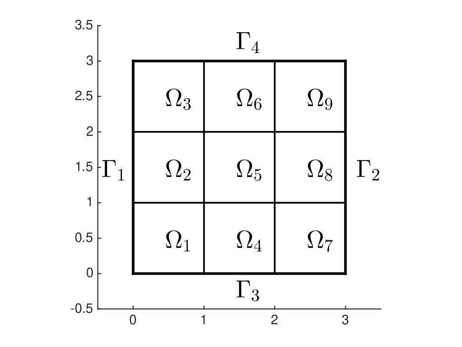
where $\Omega=\bigcup_{i=1}^{9}\,\Omega_{i}$ , and
	$\kappa(x,\mu)=\left\{\begin{array}[]{ll}1&\mbox{in}\,\Omega_{1},\\ \mu_{i}&\mbox{in}\,\Omega_{i+1},\;i=1,\ldots,8;\\ \end{array}\right.\hskip 20.00003ptg(x)=\left\{\begin{array}[]{ll}1&\mbox{on}\,\Gamma_{1},\\ 0&\mbox{on}\,\Gamma_{2},\\ 1-2x_{1}&\mbox{on}\,\Gamma_{3}.\\ \end{array}\right.$	(30c)
Furthermore, we endow $\mathcal{X}$ with the inner product
	$(w,v)=\mathcal{Q}^{\rm hf}(\nabla w\cdot\nabla v+wv).$
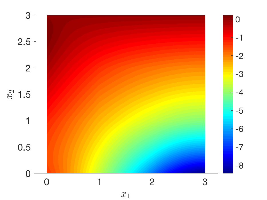
Figure 1(a) shows the computational domain, and the partition $\{\Omega_{i}\}_{i=1}^{9}$ ; while Figure 1(b) shows the behavior of the solution $u$ for a given value of $\mu\in\mathcal{P}$ . We rely on a $P=3$ Finite Element (FE) discretization ( $\mathcal{N}=8281$ , $\mathcal{N}_{\rm q}=34200$ ). Simulations are performed in Matlab $2017$ b on a Desktop computer (RAM 16Gb, 800 Mhz, Processor Intel Xeon 3.60GHz, 8 cores).

We here consider two choices for $\Phi$ :

\Phi_{1}(u)=\log\left(1+e^{u+4}\right),\hskip 10.00002pt\Phi_{2}(u)=\max\{u+4,0\}.

(30d)

In statistics and Machine Learning (see, e.g., [25]), $\Phi_{1}$ is known as logistic loss, while $\Phi_{2}$ is known as Hinge loss; as shown in Figure 1(c), $\Phi_{1}$ is a smooth approximation of $\Phi_{2}$ . Our choice is motivated by the need to investigate performance for both smooth fields and relatively rough fields: we have indeed that $\Phi_{1}\in C^{\infty}(\mathbb{R})$ , while $\Phi_{2}\in{\rm Lipschitz}(\mathbb{R})$ .

We present results for five approaches: an EIM-based ATI approach, an EIM-based ATI+ES approach (see Remark 3.2), $\ell^{1}$ -EQ+ES, EIM-EQ+ES and MIO-EQ+ES. The empirical test space is generated using the snapshot set $\{\Phi(u(\cdot;\mu^{\ell}))\}_{\ell=1}^{n_{\rm train}^{\rm es}}$ where $\mu^{1},\ldots,\mu^{n_{\rm train}^{\rm es}}$ $\overset{\rm iid}{\sim}$ ${\rm Uniform}(\mathcal{P})$ , $n_{\rm train}^{\rm es}=200$ ; similarly, the approximation space associated with EIM is generated using the same snapshot set (see Algorithm 3 in Appendix B for further details). To generate the EQ rule, we impose the accuracy constraints in $\Xi^{\rm train,eq}=\{\mu^{\ell}\}_{\ell=1}^{n_{\rm train}^{\rm eq}}$ with $n_{\rm train}^{\rm eq}=50$ ; furthermore, we use the divide-and-conquer approach discussed in section 2.3.4 with $N_{\rm part}=40$ : to speed up computations, local sparse representation problems (see (20)) are solved using $\ell^{1}$ for both $\ell^{1}$ -EQ+ES and MIO-EQ+ES. Moreover, we impose the threshold $T_{\rm max}=1800[\rm s]$ for the maximum run time of MIO-EQ+ES. For $\ell^{1}$ -EQ+ES, we rely on the Matlab routine linprog to solve the LP problem with default initial condition; for MIO-EQ+ES, we rely on intlinprog and we consider the $\ell^{1}$ -EQ+ES solution as initial condition for the optimizer. On the other hand, performance is measured using $\{\Phi(u(\cdot;\tilde{\mu}^{\ell}))\}_{\ell=1}^{n_{\rm test}}$ , where $\tilde{\mu}^{1},\ldots,\tilde{\mu}^{n_{\rm test}}$ $\overset{\rm iid}{\sim}$ ${\rm Uniform}(\mathcal{P})$ , $n_{\rm test}=100$ .

Figure 2 shows the behavior of the maximum out-of-sample error $\max_{k}\,L(\tilde{\mu}^{k})-L_{J_{\rm es}}(\tilde{\mu}^{k})$ and compares it with the squared best-fit error $\max_{k}\|\Pi_{\mathcal{X}^{\perp}_{J_{\rm es}}}\xi_{\mu}\|_{\mathcal{X}}^{2}$ , for the two choices of $\Phi$ considered. We observe that $L(\tilde{\mu}^{k})-L_{J_{\rm es}}(\tilde{\mu}^{k})\sim C\|\Pi_{\mathcal{X}_{J_{\rm es}}^{\perp}}\xi_{\mu}\|_{\mathcal{X}}^{2}$ : this is in good agreement with Eq. (25) of Proposition 2.2. We further observe that convergence with ${J_{\rm es}}$ is extremely rapid for both $\Phi=\Phi_{1}$ and $\Phi=\Phi_{2}$ .

Figures 3 show results for the five procedures: for $\ell^{1}$ -EQ+ES and MIO-EQ+ES, we impose the non-negativity constraint. Here, $\mathcal{C}_{\rm on}$ denotes the number of floating points loaded during the online stage for the different methods: note that $\mathcal{C}_{\rm on}=M^{2}$ for ATI, $\mathcal{C}_{\rm on}=MJ_{\rm es}$ for ATI+ES, and $\mathcal{C}_{\rm on}=J_{\rm es}Q_{\rm eq}$ for EQ+ES. On the other hand, $E_{\rm test}^{(\infty)}$ is the maximum prediction error over the test set:

E_{\rm test}^{(\infty)}:=\max_{k=1,\ldots,n_{\rm test}}\,\big|L(\tilde{\mu}^{k})\,-\,\widehat{L}(\tilde{\mu}^{k})\big|,

(31)

where $\widehat{L}(\cdot)$ denotes the predicted dual norm. For ATI, we show results for $M=1,2,\ldots,120$ ; for EQ+ES we show results for several prescribed tolerances — $\delta=[10^{-2},10^{-3},10^{-4},10^{-5},10^{-6}]$ for $\Phi=\Phi_{1}$ and $\delta=[10^{-2},10^{-3},5\cdot 10^{-4},10^{-4}]$ for $\Phi=\Phi_{2}$ — and two values of $J_{\rm es}$ , $J_{\rm es}=10,15$ . We recall (cf. Remark 3.2) that for $J_{\rm es}\geq M$ ATI+ES is equivalent to ATI; therefore, we set $J_{\rm es,M}={\rm min}(M,J_{\rm es})$ .

Some comments are in order. We observe that in all our examples ATI+ES is superior to the standard ATI approach: for $J_{\rm es}\gtrsim 10$ , discretization error associated with the empirical test space is negligible compared to the error $|L(\mu)-L_{M}(\mu)|$ . This also explains why increasing $J_{\rm es}$ from $10$ to $15$ does not lead to any significant improvement in accuracy. We further observe that ATI+ES significantly outperforms the three EQ+ES procedures considered for $\Phi=\Phi_{1}$ (smooth case), while ATI and ATI+ES approaches are less accurate than $\ell^{1}$ -EQ+ES and MIO-EQ+ES for most choices of the discretization parameters for $\Phi=\Phi_{2}$ (rough case). These results suggest that EQ procedures might guarantee better performance for irregular parametric functions $\Phi$ , particularly for small tolerances. Finally, we note that $\ell^{1}$ -EQ+ES and MIO-EQ+ES lead to similar performance, for both choices of $\Phi$ and for all choices of the discretization parameters, while EIM-EQ+ES is less accurate for the rough test case.

In Table 1, we report representative offline costs of dual norm estimation procedures; to facilitate interpretation, we separate sampling costs associated with the computation of $\{\Phi(u(\cdot;\mu^{\ell}))\}_{\ell=1}^{n_{\rm train}^{\rm es}=n_{\rm train}}$ — which are shared by all methods — from the other offline costs. ATI and ATI+ES are less expensive than $\ell^{1}$ -EQ, EIM-EQ+ES and MIO-EQ+ES; however, due to the overhead associated with the sampling cost, costs of ATI, ATI+ES, $\ell^{1}$ -EQ, EIM-EQ+ES are of the same order magnitude. On the other hand, MIO-EQ+ES is considerably more expensive.

Table 1: representative costs of dual norm estimation procedures; we separate sampling costs from the other costs.

Method	elapsed cost [s]
ATI ( $M=120$ )	$10.40$ + $0.60$
ATI+ES ( $M=120,J_{\rm es}=10$ )	$10.40$ + $1.08$
$\ell^{1}$ EQ+ES ( $\delta=10^{-6},J_{\rm es}=10$ , pos. weights)	$10.40$ + $26.12$
MIO EQ+ES ( $\delta=10^{-6},J_{\rm es}=10$ , pos. weights)	$10.40$ + $1800$
EIM EQ+ES ( $Q_{\rm eq}=200,J_{\rm es}=10$ )	$10.40$ + $4.85$

In Figure 4, we show results for $\ell^{1}$ -EQ+ES and MIO-EQ+ES for both non-negative weights and for real-valued weights. We observe that considering real-valued weights leads to a slight improvement in performance, particularly for $\Phi=\Phi_{2}$ .

In Figure 5, we investigate performance of $\ell^{1}$ -EQ+ES with positive weights for $\Phi=\Phi_{1},\Phi_{2}$ , for several values of $J_{\rm es}$ . We observe that for small values of $J_{\rm es}$ , the “ $J_{\rm es}$ -error” associated with ES dominates; as $J_{\rm es}$ increases, $E_{\rm test}^{(\infty)}$ reaches a threshold that depends on the value of the quadrature tolerance $\delta$ . We further observe that $Q_{\rm eq}$ grows linearly with $J_{\rm eq}$ : this is in good agreement with the result in Proposition 3.2.

Figure 6 shows the interpolation points selected by EIM, and the quadrature points obtained by applying MIO-EQ with $\delta=10^{-4}$ and real-valued weights. Interestingly, we observe that the qualitative pattern of the points selected by the two procedures is extremely similar.

4.2 Application to residual calculations

4.2.1 Problem statement

We apply the ATI+ES and EQ+ES approaches to the computation of the time-averaged residual indicator proposed in [20] for the unsteady incompressible Navier-Stokes equations. We refer to [20] for all the details concerning the definition of the model problem (a two-dimensional lid-driven cavity flow problem over a range of Reynolds numbers), and the Reduced Order Model (ROM) employed; here, we only introduce quantities that are directly related to the residual indicator. Given $\Omega=(-1,1)^{2}$ and the time grid $\{t^{j}=j\Delta t\}_{j=0}^{J}$ , we define the space $V_{\rm div}=\{v\in[H_{0}^{1}(\Omega)]^{2}:\,\nabla\cdot v\equiv 0\}$ . Then, for any sequence $\{w^{j}\}_{j=0}^{J}\subset V_{\rm div}$ we define the time-averaged residual

	$\langle R\rangle\left(\{w^{j}\}_{j=0}^{J},v;{\rm Re}\right)=\frac{\Delta t}{T-T_{0}}\,\sum_{j=J_{0}}^{J-1}\,e(w^{j},w^{j+1},v;{\rm Re}),$	(32a)
where ${\rm Re}\in\mathcal{P}=[15000,25000]$ denotes the Reynolds number, $T=t^{J},T_{0}=t^{J_{0}}$ and $e:V_{\rm div}\times V_{\rm div}\times V_{\rm div}\to\mathbb{R}$ is the residual associated with the discretized Navier-Stokes equations at time $t^{j}$
	$\begin{array}[]{rl}e(w^{j},w^{j+1},v;{\rm Re})=&\int_{\Omega}\,\left(\frac{w^{j+1}-w^{j}}{\Delta t}\,+\,(w^{j}+R_{g})\cdot\nabla(w^{j+1}+R_{g})\right)\cdot v\\[8.53581pt] &\displaystyle{+\frac{1}{\rm Re}\,\nabla\left(w^{j+1}+R_{g}\right):\nabla v\,dx.}\\ \end{array}$	(32b)
Finally, $R_{g}\in[H^{1}(\Omega)]^{2}$ , $\nabla\cdot R_{g}\equiv 0$ is a suitable lift associated with the Dirichlet boundary condition $g\in[H^{1/2}(\partial\Omega)]^{2}$ .

Our goal is to compute the dual norm of the residual $\langle R\rangle$ ,

\Delta^{\rm u}\left(\{w^{j}\}_{j=0}^{J};{\rm Re}\right):=\|\langle R\rangle\left(\{w^{j}\}_{j=0}^{J},\cdot;{\rm Re}\right)\|_{V_{\rm div}^{\prime}}

(33)

for a given ROM ${\rm Re}\in\mathcal{P}\mapsto\{\hat{u}^{j}({\rm Re})\}_{j}$ satisfying $\hat{u}^{j}(x;{\rm Re})=\sum_{n=1}^{N}\,a_{n}^{j}({\rm Re})$ $\zeta_{n}^{\rm rom}(x)$ . For this class of ROMs, we introduce the parameterized functional $\widetilde{\langle R\rangle}$ associated with $\langle R\rangle$ ,

	$\widetilde{\langle R\rangle}\,(v;{\rm Re})=\langle R\rangle\left(\{\hat{u}^{j}({\rm Re})\}_{j},\,v;{\rm Re}\right)=\int_{\Omega}\,\Upsilon(x;{\rm Re})\,\cdot\,F(x;v)\,dx$	(34a)
where $F(\cdot;v)=[(\nabla v_{1})_{1},(\nabla v_{1})_{2},(\nabla v_{2})_{1},(\nabla v_{2})_{2},v_{1},v_{2}]$ and $\Upsilon=[\Psi_{1,1},\ldots\Psi_{2,2},\Phi_{1},\Phi_{2}]$ , with
	$\begin{array}[]{rl}\Psi(\cdot;{\rm Re})=&\displaystyle{\frac{1}{\rm Re}\,\sum_{n=1}^{N}\,a_{n}^{+}\,\nabla\zeta_{n}^{\rm rom}+\nabla R_{g},}\\[8.53581pt] \Phi(\cdot;{\rm Re})=&\displaystyle{\sum_{n=1}^{N}\,\left(\frac{a_{n}^{J}-a_{n}^{J_{0}}}{T-T_{0}}\right)\,\zeta_{n}^{\rm rom}\,+\,a_{n}^{+}\,\left(R_{g}\cdot\nabla\right)\zeta_{n}^{\rm rom}\,+\,a_{n}^{-}\,\left(\zeta_{n}^{\rm rom}\cdot\nabla\right)R_{g}}\\[8.53581pt] &\displaystyle{+\,\sum_{m,n=1}^{N}\,\bar{c}_{m,n}\left(\zeta_{n}^{\rm rom}\cdot\nabla\right)\zeta_{m}^{\rm rom}\,+\,\left(R_{g}\cdot\nabla\right)R_{g}},\\ \end{array}$	(34b)
and
	$a_{n}^{+}=\frac{\Delta t}{T-T_{0}}\sum_{j=J_{0}+1}^{J}\,a_{n}^{k},\hskip 10.00002pta_{n}^{-}=\frac{\Delta t}{T-T_{0}}\sum_{j=J_{0}}^{J-1}\,a_{n}^{j},\hskip 10.00002pt\bar{c}_{m,n}=\frac{\Delta t}{T-T_{0}}\sum_{j=J_{0}}^{J-1}\,a_{m}^{j+1}\,\,a_{n}^{j}.$	(34c)
Note that the functional $\widetilde{\langle R\rangle}$ is parametrically affine; however, the number of expansion’s terms $M_{\rm R}$ is equal to $N^{2}+3N+2$ , and is thus extremely large for practical values of $N$ .

The functional $\widetilde{\langle R\rangle}$ (34) is of the form studied in this paper; for this reason, we can apply the techniques presented in sections 2 and 3 to estimate its dual norm. We consider $T=10^{3}$ , $T_{0}=500$ , $\Delta t=5\cdot 10^{-3}$ , and we consider the constrained Galerkin ROM proposed in [20] anchored in ${\rm Re}=20000$ , for two values of the ROM dimension $N$ . The high-fidelity discretization is based on a P=8 spectral element discretization with $\mathcal{N}=25538$ degrees of freedom and $\mathcal{N}_{\rm hf}=36864$ quadrature points.

4.2.2 Numerical results

We consider EIM-based ATI(+ES) and $\ell^{1}$ -EQ+ES to approximate the dual norm of $\widetilde{\langle R\rangle}$ . To generate the empirical test space, we use $n_{\rm train}^{\rm es}=150$ uniformly-sampled Reynolds numbers ${\rm Re}^{1},\ldots,{\rm Re}^{\rm n_{\rm train}}$ in $\mathcal{P}$ . Then, to generate the EQ rule, we consider the tolerance $\delta=10^{-7}$ , we impose the accuracy constraints for $n_{\rm train}^{\rm eq}=50$ parameters, and we use the divide-and-conquer strategy discussed in section 2.3.4 with $N_{\rm part}=32$ . On the other hand, to generate the ATI approximation we employ the same training set used for the generation of the empirical test space. Numerical results are presented for $M=50$ and $M=100$ , and $J_{\rm es}=50$ . Note that for $M=J_{\rm es}$ we have an exact ATI approximation. To assess performance, we consider $n_{\rm test}=11$ equispaced parameters.

Figure 7 shows the behavior of $E_{J_{\rm es}}^{\infty,\rm rel}=\max_{\rm Re}\,\frac{\|\Pi_{\mathcal{X}_{J_{\rm es}^{\perp}}}\xi_{\rm Re}\|_{\mathcal{X}}}{\|\xi_{\rm Re}\|_{\mathcal{X}}}$ over the training set and over the test set, for two values of $N$ . Note that for $J_{\rm es}\gtrsim 50$ the relative error is below $\mathcal{O}(10^{-1})$ .

Figure 8 shows the behavior of the truth and estimated error indicator $\Delta^{\rm u}({\rm Re})$ over the test set, for two values of the ROM dimension $N$ , $N=60,80$ . We observe that both ATI+ES and $\ell^{1}$ -EQ+ES lead to similar performance in terms of accuracy. $\ell^{1}$ -EQ+ES returns a quadrature rule with $Q_{\rm eq}=717$ points for $N=60$ and $Q_{\rm eq}=720$ points for $N=80$ : $\ell^{1}$ -EQ+ES thus requires the offline computation of $n_{\rm train}^{\rm es}=150$ Riesz elements and the online storage cost of $\mathcal{C}_{\rm on}=DJ_{\rm es}Q_{\rm eq}\approx 2.2\cdot 10^{5}$ floating points⁶⁶ 6 Computational cost associated with the construction of the EQ rule is here negligible compared to the other offline costs. . On the other hand, ATI(+ES) requires the computation of $n_{\rm train}^{\rm es}=150$ Riesz elements and the online storage of $\mathcal{C}_{\rm on}=MJ_{\rm es}D=0.3\cdot 10^{5}$ floating points: memory costs of ATI+ES for this test case are significantly lower than the costs of $\ell^{1}$ -EQ+ES.

We conclude by commenting on the computational savings of the here-presented approaches compared to the approach employed in [20]. In [20], the authors exploit the fact that $\widetilde{\langle R\rangle}$ (34) is parametrically affine to compute the truth dual norm. For $N=80$ , the procedure in [20] requires the offline computation and the storage of $M_{\rm R}=6642$ Riesz elements and the online storage of $\mathcal{C}_{\rm on}=M_{\rm R}^{2}=4.4\cdot 10^{7}$ floating points. Therefore, both $\ell^{1}$ -EQ+ES and ATI+ES dramatically reduce offline and online memory costs. As regards the online computational cost, computation of the residual indicator involves the computation of the $\mathcal{O}(N^{2})$ coefficients in (34), which requires $\mathcal{O}(N^{2}(J-J_{0}))$ flops. Since $J-J_{0}\approx 10^{5}\gg N^{2}$ , the online cost is dominated by the computation of the parameter-dependent coefficients in (34) for both approaches: as a result, the benefit of EQ+ES and ATI+ES in terms of online computational savings is extremely modest for the problem at hand.

5 Conclusions

In this paper, we developed and analyzed an offline/online computational procedure for computing the dual norm of parameterized linear functionals. The key elements are an Empirical test Space (ES) built using POD, which reduces the dimensionality of the optimization problem associated with the computation of the dual norm, and an Empirical Quadrature (EQ) procedure based on an $\ell^{1}$ relaxation or on MIO, which allows efficient calculations in an offline/online setting.

We presented theoretical and numerical results to justify our approach. In particular, our results suggest that resorting to ES for proper choices of $J_{\rm es}$ might significantly reduce computational and memory costs without affecting accuracy. Furthermore, for the problem at hand, ATI was clearly superior for smooth integrands, while EQ strategies were able to achieve better accuracies for a non-differentiable integrand. Finally, the performance of $\ell^{1}$ -EQ+ES was inferior to that of an ATI+ES approach for the estimation of the time-averaged residual indicator proposed in [20].

We believe that several aspects of the proposed approach deserve further investigations. First, we wish to extend the analysis to quadrature rules with positive weights, and we wish to study the performance of the divide-and-conquer approach presented in section 2.3. Second, we envision that our approach could also be employed to reduce memory and computational costs associated with minimum residual ROMs ([13, 36]) for nonlinear problems.

Appendix A Notation

High-fidelity discretization

$\mathcal{X}={\rm span}\{\varphi_{i}\}_{i=1}^{\mathcal{N}}$	ambient space defined over $\Omega\subset\mathbb{R}^{d}$
$\mathcal{X}^{\prime}$	dual space
$R_{\mathcal{X}}:\mathcal{X}^{\prime}\to\mathcal{X}$	Riesz operator
$\Pi_{\mathcal{W}}:\mathcal{X}\to\mathcal{W}$	orthogonal projector operator onto the linear space $\mathcal{W}\subset\mathcal{X}$
$\mathcal{Q}^{\rm hf}(v)=\sum_{i=1}^{\mathcal{N}_{\rm q}}\,\rho_{i}^{\rm hf}\,v(x_{i}^{\rm hf})$	high-fidelity quadrature rule
$\mathbf{v}\in\mathbb{R}^{\mathcal{N}}$	vector of coefficients such that $v=\sum_{i}v_{i}\,\varphi_{i}$
$\boldsymbol{\mathcal{L}}\in\mathbb{R}^{\mathcal{N}}$	vector $\boldsymbol{\mathcal{L}}=[\mathcal{L}(\varphi_{1}),\ldots,\mathcal{L}(\varphi_{\mathcal{N}})]$ for any $\mathcal{L}\in\mathcal{X}^{\prime}$
$\mathbb{X}\in\mathbb{R}^{\mathcal{N}\times\mathcal{N}}$	matrix such that $\mathbb{X}_{i,j}=(\varphi_{j},\varphi_{i})_{\mathcal{X}}$
$C_{\rm riesz}=\mathcal{O}(\mathcal{N}^{s})$	cost to compute $R_{\mathcal{X}}\mathcal{L}$ for a given $\mathcal{L}\in\mathcal{X}^{\prime}$

Parameterized functional

$\mu\in\mathcal{P}\subset\mathbb{R}^{P}$	vector of parameters
$F(\cdot;v):\Omega\to\mathbb{R}^{D}$	linear function of $v$ and its derivatives
	(e.g., $F(x;v)=[v(x),\nabla v(x)]$ )
$\Upsilon_{\mu}:\Omega\to\mathbb{R}^{D}$	parameterized function
$\mathcal{L}_{\mu}(v)=\mathcal{Q}^{\rm hf}(\eta(\cdot;v,\mu))$	parameterized functional with $\eta(x;v,\mu)=\Upsilon_{\mu}(x)\cdot F(x;v)$
$L(\mu)=\\|\mathcal{L}_{\mu}\\|_{\mathcal{X}^{\prime}}$	dual norm
$\xi_{\mu}=R_{\mathcal{X}}\mathcal{L}_{\mu}$	Riesz element of $\mathcal{L}_{\mu}$
$\mathcal{M}_{\mathcal{L}}=\{\xi_{\mu}:\mu\in\mathcal{P}\}$	dual norm

EQ+ES discretization

$\mathcal{X}_{J_{\rm es}}={\rm span}\{\phi_{j}\}_{j=1}^{J_{\rm es}}$	empirical test space
$\mathcal{Q}^{\rm eq}(v)=\sum_{q=1}^{Q_{\rm eq}}\,\rho_{q}^{\rm eq}\,v(x_{q}^{\rm eq})$	empirical quadrature rule
$L_{J_{\rm es},Q_{\rm eq}}(\mu)=\sup_{\phi\in\mathcal{X}_{J_{\rm es}}}\,\frac{\mathcal{Q}^{\rm eq}(\eta(\cdot;\phi,\mu))}{\\|\phi\\|_{\mathcal{X}}}$	EQ+ES dual norm estimate
$L_{J_{\rm es}}(\mu)=\\|\mathcal{L}_{\mu}\\|_{\mathcal{X}_{J_{\rm es}}}$	ES dual norm estimate
$\Xi^{\rm train,es}=\{\mu^{\ell}\}_{\ell=1}^{n_{\rm train}^{\rm es}}\subset\mathcal{P}$	parameter training set for $\mathcal{X}_{J_{\rm es}}$ generation
$\Xi^{\rm train,eq}=\{\mu^{\ell}\}_{\ell=1}^{n_{\rm train}^{\rm eq}}\subset\mathcal{P}$	parameter training set associated with (10)
$K=n_{\rm train}^{\rm eq}J_{\rm eq}+1$	number of rows in $\mathbb{G}$ in (13)

ATI discretization

$\Upsilon_{M,\mu}(x)=\sum_{m=1}^{M}\,\left(\boldsymbol{\Theta}_{M}(\mu)\right)_{m}\zeta_{m}(x)$	$M$ -term affine approximation of $\Upsilon_{\mu}$
$\mathcal{L}_{M,\mu}(v)=\mathcal{Q}^{\rm hf}(\eta_{M}(\cdot;v,\mu))$	$M$ -term affine approximation of $\mathcal{L}_{\mu}$
	$\eta_{M}(x;v,\mu):=\Upsilon_{M,\mu}(x)\cdot F(x;v)$
$L_{M}(\mu)=\\|\mathcal{L}_{M,\mu}\\|_{\mathcal{X}^{\prime}}$	ATI dual norm estimate
$L_{M,J_{\rm es}}(\mu)=\\|\mathcal{L}_{M,\mu}\\|_{\mathcal{X}_{J_{\rm es}}^{\prime}}$	ATI+ES dual norm estimate

Appendix B Empirical Interpolation Method

B.1 Review of the interpolation procedure for scalar fields

We review the Empirical Interpolation Method (EIM), and we discuss its application to empirical quadrature and its extension to the approximation of vector-valued fields. Given the Hilbert space $\mathcal{Y}$ defined over $\Omega$ , the $M$ -dimensional linear space $\mathcal{Z}_{M}={\rm span}\{\psi_{m}\}_{m=1}^{M}\subset\mathcal{Y}$ and the points $\{x_{m}^{\rm i}\}_{m=1}^{M}\subset\overline{\Omega}$ , we define the interpolation operator $\mathcal{I}_{M}:\mathcal{Y}\to\mathcal{Z}_{M}$ such that $\mathcal{I}_{M}(v)(x_{m}^{\rm i})=v(x_{m}^{\rm i})$ for $m=1,\ldots,M$ for all $v\in\mathcal{Y}$ . Given the manifold $\mathcal{F}\subset\mathcal{Y}$ and an integer $M>0$ , the objective of EIM is to determine an approximation space $\mathcal{Z}_{M}$ and $M$ points $\{x_{m}^{\rm i}\}_{m=1}^{M}$ such that $\mathcal{I}_{M}(f)$ accurately approximates $f$ for all $f\in\mathcal{F}$ .

Algorithm 3 summarizes the EIM procedure as implemented in our code. The algorithm takes as input snapshots of the manifold $\{f^{k}\}_{k=1}^{n_{\rm train}}\subset\mathcal{F}$ and returns the functions $\{\psi_{m}\}_{m=1}^{M}$ , the interpolation points $\{x_{m}^{\rm i}\}_{m=1}^{M}$ and the matrix $\mathbb{B}\in\mathbb{R}^{M\times M}$ such that $\mathbb{B}_{m,m^{\prime}}=\psi_{m}(x_{m^{\prime}}^{\rm i})$ . It is possible to show that the matrix $\mathbb{B}$ is lower-triangular: for this reason, online computations can be performed in $\mathcal{O}(M^{2})$ flops. Note that in the original EIM paper the authors resort to a strong Greedy procedure to generate $\mathcal{Z}_{M}$ , while here (as in several other works including [14]) we resort to POD. A thorough comparison between the two compression strategies is beyond the scope of the present work.

Algorithm 3 Empirical Interpolation Method.

Inputs:	$\{f^{k}\}_{k=1}^{n_{\rm train}}$ , $M$
Outputs:	$\{\psi_{m}\}_{m=1}^{M},\mathbb{B}\in\mathbb{R}^{M\times M},\{x_{m}^{\rm i}\}_{m=1}^{M}$

1: Build the POD space

\zeta_{1},\ldots,\zeta_{M}

based on the snapshot set

\{f^{k}\}_{k=1}^{n_{\rm train}}

x_{1}^{\rm i}:={\rm arg}\max_{x\in\overline{\Omega}}\,|\psi_{1}(x)|

\psi_{1}:=\frac{1}{\zeta_{1}(x_{1}^{\rm i})}\,\zeta_{1}

\left(\mathbb{B}\right)_{1,1}=1

3: for

m=2,\ldots,M

r_{m}=\zeta_{m}-\mathcal{I}_{m-1}\zeta_{m}

x_{m}^{\rm i}:={\rm arg}\max_{x\in\overline{\Omega}}\,|r_{m}(x)|

\psi_{m}=\frac{1}{r_{m}(x_{m}^{\rm i})}\,r_{m}

\left(\mathbb{B}\right)_{m,m^{\prime}}=\psi_{m}(x_{m^{\prime}}^{\rm i})

6: end for

B.2 Application to empirical quadrature

As shown in [2], EIM naturally induces a specialized quadrature rule for elements of $\mathcal{F}$ . To show this, we consider the approximation:

\mathcal{Q}^{\rm hf}\left(f\right)\approx\mathcal{Q}^{\rm hf}\left(\mathcal{I}_{M}(f)\right)=\sum_{m,m^{\prime}=1}^{M}\mathcal{Q}^{\rm hf}\left(\psi_{m}\right)\mathbb{B}_{m,m^{\prime}}^{-1}\,f(x_{m^{\prime}}^{\rm i})=\sum_{m^{\prime}=1}^{M}\rho_{m^{\prime}}^{\rm eq}\,f(x_{m^{\prime}}^{\rm i})

where $\rho_{m^{\prime}}^{\rm eq}=\sum_{m=1}^{M}\mathbb{B}_{m,m^{\prime}}^{-1}\mathcal{Q}^{\rm hf}\left(\psi_{m}\right)$ . Note that in the first equality we used $\mathcal{I}_{M}(f)(x)=\sum_{m,m^{\prime}=1}^{M}\,\mathbb{B}_{m,m^{\prime}}^{-1}\,\,f(x_{m^{\prime}}^{\rm i})\psi_{m}(x)$ .

B.3 Extension to vector-valued fields

The EIM procedure can be extended to vector-valued fields. We present below the non-interpolatory extension of EIM employed in section 4.2. We refer to [33, 26] for two alternatives applicable to vector-valued fields. Given the space $\mathcal{Z}_{M}={\rm span}\{\zeta_{m}\}_{m=1}^{M}\subset\mathcal{Y}$ and the points $\{x_{m}^{\rm i}\}_{m=1}^{M}\subset\overline{\Omega}$ , we define the least-squares approximation operator $\mathcal{I}_{M}:\mathcal{Y}\to\mathcal{Z}_{M}$ such that for all $v\in\mathcal{Y}$

\mathcal{I}_{M}(v):={\rm arg}\min_{\zeta\in\mathcal{Z}_{M}}\,\sum_{m=1}^{M}\,\|v(x_{m}^{\rm i})-\zeta(x_{m}^{\rm i})\|_{2}^{2}.

It is possible to show that $\mathcal{I}_{M}$ is well-defined if and only if the matrix $\mathbb{B}\in\mathbb{R}^{MD\times M}$ ,

	$\mathbb{B}=\left[\begin{array}[]{ccc}\zeta_{1}(x_{1}^{\rm i}),&\ldots,&\zeta_{M}(x_{1}^{\rm i})\\ &\vdots&\\ \zeta_{1}(x_{M}^{\rm i}),&\ldots,&\zeta_{M}(x_{M}^{\rm i})\\ \end{array}\right]$	(35a)
is full-rank. In this case, we find that $\mathcal{I}_{M}$ can be efficiently computed as
	$\mathcal{I}_{M}(v)=\sum_{m=1}^{M}\,\left(\boldsymbol{\alpha}(v)\right)_{m}\,\zeta_{m},\hskip 10.00002pt\boldsymbol{\alpha}(v)=\mathbb{B}^{\dagger}\left[\begin{array}[]{c}v(x_{1}^{\rm i})\\ \vdots\\ v(x_{M}^{\rm i})\\ \end{array}\right]$	(35b)
for any $v\in\mathcal{Y}$ , where $\mathbb{B}^{\dagger}=(\mathbb{B}^{T}\mathbb{B})^{-1}\mathbb{B}^{T}$ denotes the Moore-Penrose pseudo-inverse of $\mathbb{B}$ .

Algorithm 4 summarizes the procedure employed to compute $\mathcal{Z}_{M}$ , $\{x_{m}^{\rm i}\}_{m=1}^{M}$ and the matrix $\mathbb{B}$ . We observe that for scalar fields the procedure reduces to the one outlined in Algorithm 3. We further observe that online computational cost scales with $\mathcal{O}(DM^{2})$ , provided that $\mathbb{B}^{\dagger}$ is computed offline.

Algorithm 4 Empirical Interpolation Method for vector-valued fields.

Inputs:	$\{f^{k}\}_{k=1}^{n_{\rm train}}$ , $M$
Outputs:	$\{\zeta_{m}\}_{m=1}^{M},\mathbb{B}^{\dagger}\in\mathbb{R}^{M\times M},\{x_{m}^{\rm i}\}_{m=1}^{M}$

1: Build the POD space

\zeta_{1},\ldots,\zeta_{M}

based on the snapshot set

\{f^{k}\}_{k=1}^{n_{\rm train}}

2: Set

x_{1}^{\rm i}:={\rm arg}\max_{x\in\overline{\Omega}}\,\|\zeta_{1}(x)\|_{2}

, and

\mathbb{B}_{M=1}

using (35).

3: for

m=2,\ldots,M

r_{m}=\zeta_{m}-\mathcal{I}_{m-1}\zeta_{m}

5: Set

x_{m}^{\rm i}:={\rm arg}\max_{x\in\overline{\Omega}}\,\|r_{m}(x)\|_{2}

, and update

\mathbb{B}_{M=m}

using (35).

6: end for

7: Compute

\mathbb{B}^{\dagger}=(\mathbb{B}^{T}\mathbb{B})^{-1}\mathbb{B}

Appendix C Proof of Proposition 3.2

In view of the proof of Proposition 3.2, we need the following Lemma.

Lemma C.1.

Let $\mathcal{W}_{N}={\rm span}\{w_{n}\}_{n=1}^{N}\subset C(\bar{\Omega})$ be a $N$ -dimensional space. Then, there exist $x_{1}^{o},\ldots,x_{N}^{o}\in\bar{\Omega}$ and $\psi_{1},\ldots,\psi_{N}$ such that $\psi_{n}(x_{n^{\prime}}^{o})=\delta_{n,n^{\prime}}$ $n,n^{\prime}=1,\ldots,N$ , and

w(x)=\sum_{n=1}^{N}\,w(x_{n}^{o})\,\psi_{n}(x)\hskip 10.00002pt\forall\,x\in\Omega,\hskip 10.00002pt\forall\,w\in\mathcal{W}_{N}.

(36)

Similarly, given the matrix $\mathbb{G}\in\mathbb{R}^{K\times\mathcal{N}_{\rm q}}$ such that ${\rm rank}(\mathbb{G})=N$ , there exist $\mathbb{A}\in\mathbb{R}^{K\times N}$ , $\mathbb{B}\in\mathbb{R}^{N\times\mathcal{N}_{\rm q}}$ and $\mathcal{I}_{N}\subset\{1,\ldots,\mathcal{N}_{\rm q}\}$ such that

\mathbb{G}=\mathbb{A}\mathbb{B},\hskip 10.00002pt\mathbb{B}(:,\mathcal{I}_{N})=\mathbb{I}_{N}.

(37)

Proof.

Proofs of (36) and (37) are analogous; for this reason, we prove below (36), and we omit the proof of (37) .

We proceed by induction. For $N=1$ , if we define $x_{1}^{o}={\rm arg}\max_{x\in\bar{\Omega}}|w_{1}(x)|$ and $\psi_{1}(\cdot)=\frac{1}{w_{1}(x_{1}^{o})}w_{1}(\cdot)$ , we find $w(x)=w(x_{1}^{o})\psi_{1}(x)$ for all $x\in\Omega$ and $w\in\mathcal{W}_{N=1}$ , which is (36).

We now assume that the thesis holds for $N-1=N_{0}$ , and we prove that it holds also for $N=N_{0}+1$ . With this in mind, we consider $w=\sum_{n=1}^{N}a_{n}w_{n}$ for some $a_{1},\ldots,a_{N}\in\mathbb{R}$ . We observe that

w(x)-a_{N}w_{N}(x)=\sum_{n=1}^{N-1}\,a_{n}w_{n}(x)\hskip 10.00002pt\forall\,x\in\Omega.

Then, exploiting the fact that the result holds for $N-1=N_{0}$ , we obtain

w(x)=a_{N}w_{N}(x)+\sum_{n=1}^{N-1}\,\left(w(x_{n}^{o})-a_{N}w_{N}(x_{n}^{o})\right)\tilde{\psi}_{n}(x)=a_{N}\tilde{\psi}_{N}(x)+\sum_{n=1}^{N-1}\,w(x_{n}^{o})\tilde{\psi}_{n}(x),

where $\{x_{n}^{o}\}_{n=1}^{N-1}\subset\bar{\Omega}$ , $\tilde{\psi}_{n}(x_{n^{\prime}}^{o})=\delta_{n,n^{\prime}}$ for $n,n^{\prime}=1,\ldots,N-1$ , and $\tilde{\psi}_{N}$ is defined as

\tilde{\psi}_{N}(x)=w_{N}(x)-\sum_{n=1}^{N-1}\,w_{N}(x_{n}^{o})\,\tilde{\psi}_{n}(x).

If we define

x_{N}^{o}\in{\rm arg}\max_{x\in\bar{\Omega}}\,|\tilde{\psi}_{N}(x)|,\hskip 10.00002pt\psi_{N}(x):=\frac{1}{\psi_{N}(x_{N}^{o})}\,\psi_{N}(x),

we find that $\psi_{N}(x_{n}^{o})=\delta_{N,n}$ for $n=1,\ldots,N$ , and

\begin{array}[]{rl}w(x)=&\displaystyle{\left(w(x_{N}^{o})-\sum_{n=1}^{N-1}w(x_{n}^{o})\,\tilde{\psi}_{n}(x_{N}^{o})\right)\psi_{N}(x)\,+\,\sum_{n=1}^{N-1}w(x_{n}^{o})\,\tilde{\psi}_{n}(x)}\\[8.53581pt] =&\displaystyle{w(x_{N}^{o})\,\psi_{N}(x)\,+\,\sum_{n=1}^{N-1}w(x_{n}^{o})\left(\tilde{\psi}_{n}(x)-\tilde{\psi}_{n}(x_{N}^{o})\psi_{N}(x)\right)}\\ \end{array}

Thesis follows by defining $\psi_{n}(x):=\tilde{\psi}_{n}(x)-\tilde{\psi}_{n}(x_{N}^{o})\psi_{N}(x)$ and observing that $\psi_{n}(x_{n^{\prime}}^{o})=\delta_{n,n^{\prime}}$ for $n,n^{\prime}=1,\ldots,N$ . ∎∎

Proof.

(Proposition 3.2) We define $\eta_{M}(x;\phi,\mu):=\Upsilon_{M,\mu}(x)\cdot F(x;\phi)$ and the matrix $\mathbb{G}_{M}\in\mathbb{R}^{K\times\mathcal{N}_{\rm q}}$ such that

\mathbb{G}_{M}=\left[\begin{array}[]{ccc}\eta_{M}(x_{1}^{\rm hf};\phi_{1},\mu^{1}),&\ldots&\eta_{M}(x_{\mathcal{N}_{\rm q}}^{\rm hf};\phi_{1},\mu^{1})\\ &\vdots&\\ \eta_{M}(x_{1}^{\rm hf};\phi_{J_{\rm es}},\mu^{n_{\rm train}^{\rm eq}}),&\ldots&\eta_{M}(x_{\mathcal{N}_{\rm q}}^{\rm hf};\phi_{J_{\rm es}},\mu^{n_{\rm train}^{\rm eq}})\\[5.69054pt] 1&\ldots&1\\ \end{array}\right].

By construction, for any choice of $\Xi^{\rm train,eq}=\{\mu^{\ell}\}_{\ell=1}^{n_{\rm train}^{\rm eq}}$ , we have that

\{\eta_{M}(x;\phi_{j},\mu^{\ell})\}_{j,\ell}\cup\{1\}\subset\mathcal{W}_{N}:={\rm span}\left\{1,\,\zeta_{1}\cdot F(\cdot;\phi_{1}),\ldots,\zeta_{M}\cdot F(\cdot;\phi_{J_{\rm es}})\right\},

with ${\rm dim}(\mathcal{W}_{N})=N\leq MJ_{\rm es}+1$ . Recalling Lemma C.1, there exist $\mathbb{A}_{N,M}^{\rm train}\in\mathbb{R}^{K\times N}$ , $\mathbb{B}_{N,M}\in\mathbb{R}^{N\times\mathcal{N}_{\rm q}}$ and $\mathcal{I}_{N}\subset\{1,\ldots,\mathcal{N}_{\rm q}\}$ such that $\mathbb{G}_{M}=\mathbb{A}_{N,M}^{\rm train}\,\mathbb{B}_{N,M}$ and $\mathbb{B}_{N,M}(:,\mathcal{I}_{N})=\mathbb{I}_{N}$ .

We now introduce $\hat{\boldsymbol{\rho}}\in\mathbb{R}^{\mathcal{N}_{\rm q}}$ such that $\hat{\boldsymbol{\rho}}_{i}=0$ if $i\notin\mathcal{I}_{N}$ and $\hat{\boldsymbol{\rho}}(\mathcal{I}_{N})=:\hat{\boldsymbol{\rho}}_{N}=\mathbb{B}_{N,M}\boldsymbol{\rho}^{\rm hf}$ . Then, we find

\|{\mathbb{G}}\hat{\boldsymbol{\rho}}-\mathbf{y}^{\rm hf}\|_{\infty}=\|{\mathbb{G}}(\hat{\boldsymbol{\rho}}-\boldsymbol{\rho}^{\rm hf})\|_{\infty}\leq\underbrace{\|{\mathbb{G}}_{M}(\hat{\boldsymbol{\rho}}-\boldsymbol{\rho}^{\rm hf})\|_{\infty}}_{=\rm(I)}+\underbrace{\|({\mathbb{G}}-{\mathbb{G}}_{M})\hat{\boldsymbol{\rho}}\|_{\infty}}_{=\rm(II)}+\underbrace{\|({\mathbb{G}}-{\mathbb{G}}_{M}){\boldsymbol{\rho}}^{\rm hf}\|_{\infty}}_{=\rm(III)}

By construction, (I) $=0$ , while exploiting (29a) we find (III) $\leq\delta_{\rm ati}$ . Finally, recalling the definition of $\epsilon_{\rm ati}$ in (29b), we obtain

{\rm(II)}\leq\epsilon_{\rm ati}\|\hat{\boldsymbol{\rho}}\|_{1}=\epsilon_{\rm ati}\,\big\|\mathbb{B}_{N,M}\,\boldsymbol{\rho}^{\rm hf}\big\|_{1}

If we set $C_{M,J_{\rm es}}=\big\|\mathbb{B}_{N,M}\,\boldsymbol{\rho}^{\rm hf}\big\|_{1}$ , we obtain that $\hat{\boldsymbol{\rho}}$ is admissible and has $N\leq MJ_{\rm es}+1$ non-zero entries. Thesis follows. ∎∎

References

[1] S S An, T Kim, and D L James. Optimizing cubature for efficient integration of subspace deformations. ACM transactions on graphics (TOG), 27(5):165:1–165:10, 2008.
[2] H Antil, S E Field, F Herrmann, R H Nochetto, and M Tiglio. Two-step greedy algorithm for reduced order quadratures. Journal of Scientific Computing, 57(3):604–637, 2013.
[3] P Astrid, S Weiland, K Willcox, and T Backx. Missing point estimation in models described by proper orthogonal decomposition. IEEE Transactions on Automatic Control, 53(10):2237–2251, 2008.
[4] O Balabanov and A Nouy. Randomized linear algebra for model reduction. Part I: Galerkin methods and error estimation. arXiv preprint arXiv:1803.02602, 2018.
[5] M Barrault, Y Maday, NC Nguyen, and A T Patera. An ‘empirical interpolation’ method: application to efficient reduced-basis discretization of partial differential equations. Comptes Rendus Mathematique, 339(9):667–672, 2004.
[6] G Berkooz, P Holmes, and J L Lumley. The proper orthogonal decomposition in the analysis of turbulent flows. Annual review of fluid mechanics, 25(1):539–575, 1993.
[7] D Bertsimas, A King, and R Mazumder. Best subset selection via a modern optimization lens. The annals of statistics, 44(2):813–852, 2016.
[8] D Bertsimas and R Weismantel. Optimization over integers, volume 13. Dynamic Ideas Belmont, 2005.
[9] A M Bruckstein, D L Donoho, and M Elad. From sparse solutions of systems of equations to sparse modeling of signals and images. SIAM review, 51(1):34–81, 2009.
[10] A Buhr and K Smetana. Randomized local model order reduction. SIAM Journal on Scientific Computing (accepted), 2018.
[11] T Bui-Thanh, M Damodaran, and K Willcox. Proper orthogonal decomposition extensions for parametric applications in compressible aerodynamics. In 21st AIAA Applied Aerodynamics Conference, pages Paper 2003–4213, 2003.
[12] K Carlberg, Charbel Bou-Mosleh, and Charbel Farhat. Efficient non-linear model reduction via a least-squares Petrov–Galerkin projection and compressive tensor approximations. International Journal for Numerical Methods in Engineering, 86(2):155–181, 2011.
[13] K Carlberg, C Farhat, J Cortial, and D Amsallem. The GNAT method for nonlinear model reduction: effective implementation and application to computational fluid dynamics and turbulent flows. Journal of Computational Physics, 242:623–647, 2013.
[14] S Chaturantabut and D C Sorensen. Nonlinear model reduction via discrete empirical interpolation. SIAM Journal on Scientific Computing, 32(5):2737–2764, 2010.
[15] C Daversin-Catty and C Prud’Homme. Simultaneous empirical interpolation and reduced basis method for non-linear problems. Comptes Rendus Mathématique, 353(12):1105–1109, 2015.
[16] D L Donoho. Compressed sensing. IEEE Transactions on information theory, 52(4):1289–1306, 2006.
[17] M Drohmann, B Haasdonk, and M Ohlberger. Reduced basis approximation for nonlinear parametrized evolution equations based on empirical operator interpolation. SIAM Journal on Scientific Computing, 34(2):A937–A969, 2012.
[18] R Everson and L Sirovich. Karhunen–Loeve procedure for gappy data. Journal of the Optical Society of America A, 12(8):1657–1664, 1995.
[19] C Farhat, T Chapman, and P Avery. Structure-preserving, stability, and accuracy properties of the energy-conserving sampling and weighting method for the hyper reduction of nonlinear finite element dynamic models. International Journal for Numerical Methods in Engineering, 102(5):1077–1110, 2015.
[20] L Fick, Y Maday, A T Patera, and T Taddei. A stabilized POD model for turbulent flows over a range of Reynolds numbers: optimal parameter sampling and constrained projection. Journal of Computational Physics, 371:214 – 243, 2018.
[21] M A Grepl, Y Maday, N C Nguyen, and A T Patera. Efficient reduced-basis treatment of nonaffine and nonlinear partial differential equations. ESAIM: Mathematical Modelling and Numerical Analysis, 41(3):575–605, 2007.
[22] T Hastie, R Tibshirani, and R J Tibshirani. Extended comparisons of best subset selection, forward stepwise selection, and the Lasso. arXiv preprint arXiv:1707.08692, 2017.
[23] J S Hesthaven, G Rozza, and B Stamm. Certified reduced basis methods for parametrized partial differential equations. SpringerBriefs in Mathematics, 2015.
[24] C Himpe, T Leibner, and S Rave. Hierarchical approximate proper orthogonal decomposition. SIAM Journal on Scientific Computing, 40(5):A3267–A3292, 2018.
[25] G James, D Witten, T Hastie, and R Tibshirani. An introduction to statistical learning, volume 112. Springer, 2013.
[26] F Negri, A Manzoni, and D Amsallem. Efficient model reduction of parametrized systems by matrix discrete empirical interpolation. Journal of Computational Physics, 303:431–454, 2015.
[27] N C Nguyen, A T Patera, and J Peraire. A ‘best points’ interpolation method for efficient approximation of parametrized functions. International journal for numerical methods in engineering, 73(4):521–543, 2008.
[28] A T Patera and M Yano. An LP empirical quadrature procedure for parametrized functions. Comptes Rendus Mathematique, 355(11):1161–1167, 2017.
[29] A Quarteroni, A Manzoni, and F Negri. Reduced Basis Methods for Partial Differential Equations: An Introduction, volume 92. Springer, 2015.
[30] G Rozza, DB P Huynh, and A T Patera. Reduced basis approximation and a posteriori error estimation for affinely parametrized elliptic coercive partial differential equations. Archives of Computational Methods in Engineering, 15(3):229–275, 2008.
[31] D Ryckelynck. Hyper-reduction of mechanical models involving internal variables. International Journal for Numerical Methods in Engineering, 77(1):75–89, 2009.
[32] L Sirovich. Turbulence and the dynamics of coherent structures. I. Coherent structures. Quarterly of applied mathematics, 45(3):561–571, 1987.
[33] T Tonn. Reduced-basis method (RBM) for non-affine elliptic parametrized PDEs. PhD thesis, PhD thesis, Ulm University, 2011.
[34] J A Tropp. Greed is good: Algorithmic results for sparse approximation. IEEE Transactions on Information theory, 50(10):2231–2242, 2004.
[35] S Volkwein. Model reduction using proper orthogonal decomposition. Lecture Notes, Institute of Mathematics and Scientific Computing, University of Graz. see http://www.math.uni-konstanz.de/numerik/personen/volkwein/teaching/POD-Vorlesung.pdf, 2011.
[36] M Yano. A space-time Petrov–Galerkin certified reduced basis method: Application to the Boussinesq equations. SIAM Journal on Scientific Computing, 36(1):A232–A266, 2014.
[37] M Yano. Discontinuous Galerkin reduced basis empirical quadrature procedure for model reduction of parametrized nonlinear conservation laws, 2018.
[38] M Yano and A T Patera. An LP empirical quadrature procedure for reduced basis treatment of parametrized nonlinear PDEs. Computational Methods in Applied Mechanics and Engineering (accepted), 2018.

An offline/online procedure for dual norm calculations of parameterized functionals: empirical quadrature and empirical test spaces

Abstract

1 Introduction

2 Methodology

2.1 Formulation

Remark 2.1.

2.2 Empirical test space

Remark 2.2.

Connection with ℓ2\ell_{2}-embeddings

2.3 Empirical quadrature

Remark 2.3.

2.3.1 ℓ1\ell^{1} relaxation (ℓ1\ell^{1}-EQ)

2.3.2 Quadrature rule using EIM (EIM-EQ)

2.3.3 Solution to (14) using MIO (MIO-EQ)

2.3.4 A divide-and-conquer approach for ℓ1\ell^{1}-EQ and MIO-EQ

Proposition 2.1.

Proof.

2.4 Summary of the EQ+ES offline/online procedure

2.5 A priori error analysis

Proposition 2.2.

Proof.

3 Approximation-then-integration approaches for dual-norm calculations

3.1 Review of ATI-based approaches for dual norm calculations

Proposition 3.1.

Proof.

Remark 3.1.

Remark 3.2.

3.2 Discussion

Proposition 3.2.

4 Numerical results

4.1 Comparison between EQ+ES and an EIM-based ATI approach

4.2 Application to residual calculations

4.2.1 Problem statement

4.2.2 Numerical results

5 Conclusions

Appendix A Notation

Appendix B Empirical Interpolation Method

B.1 Review of the interpolation procedure for scalar fields

B.2 Application to empirical quadrature

B.3 Extension to vector-valued fields

Appendix C Proof of Proposition 3.2

Lemma C.1.

Proof.

Proof.

References

Connection with $\ell_{2}$ -embeddings

2.3.1 $\ell^{1}$ relaxation ( $\ell^{1}$ -EQ)

2.3.4 A divide-and-conquer approach for $\ell^{1}$ -EQ and MIO-EQ