Accelerated Bayesian Optimization through Weight-Prior Tuning
Abstract
Bayesian optimization (BO) is a widely-used method for optimizing expensive (to evaluate) problems. At the core of most BO methods is the modeling of the objective function using a Gaussian Process (GP) whose covariance is selected from a set of standard covariance functions. From a weight-space view, this models the objective as a linear function in a feature space implied by the given covariance , with an arbitrary Gaussian weight prior . In many practical applications there is data available that has a similar (covariance) structure to the objective, but which, having different form, cannot be used directly in standard transfer learning. In this paper we show how such auxiliary data may be used to construct a GP covariance corresponding to a more appropriate weight prior for the objective function. Building on this, we show that we may accelerate BO by modeling the objective function using this (learned) weight prior, which we demonstrate on both test functions and a practical application to short-polymer fibre manufacture.
1 Introduction
Bayesian Optimization (BO) [Snoek et al., 2012, Brochu et al., 2010] is a form of sequential model-based optimization (SMBO) that aims to to find with the least number of evaluations for an expensive (to evaluate) function . In many cases there exists an additional, auxiliary dataset relating to that is relevant to the problem at hand - for example patents and technical handbooks that contain condensed knowledge related to , data obtained from similar (possibly older or superseded) equipment and, more generally, results from optimizing structurally similar functions. It is not necessary that the auxiliary data be generated by (if was generated by a function sufficiently similar to then we could simply use standard transfer learning techniques [Pan and Yang, 2010, Yogatama and Mann, 2014, Bardenet et al., 2013, Joy et al., 2016, Shilton et al., 2017]); rather, what matters is that the auxiliary data is structurally similar to insofar as it has a similar covariance structure. Human experimenters routinely use such data to inform and accelerate the (experimental) optimization process. In the present paper we investigate the use of such data to accelerate Bayesian Optimization.
Typically in BO it is assumed that is a draw from a zero mean Gaussian Process (GP) [Rasmussen, 2006] with covariance . In general is unknown, so we select an alternative to use in its place. When selecting we use intuitions and experimentalist knowledge relating to - for example how smooth is (should we use squared exponential or Matérn covariance?), is the length-scale consistent everywhere (should be use an isotropic or anisotropic covariance?) etc, but typically we restrict our choice to a subset of standard kernels. This introduces approximations and experimenter biases, as our knowledge of the covariance structure of is by definition incomplete in most cases, and moreover it appears unlikely that the covariance structure can captured by a small set of generic “standard” covariance functions. Subsequently BO is likely to converge more slowly than it should as the GP used to model has an inaccurate covariance function.
To overcome the deficiencies it is standard practice to tune hyper-parameters of at each iteration of the BO, either to maximize the log-likelihood function or minimize some sort of approximation error (e.g. leave-one-out error). The auxiliary dataset may be used to accelerate the process by pre-tuning hyper-parameters or, if it is large enough, techniques such as multi-kernel learning (MKL) [Lanckriet et al., 2004, Bach et al., 2004] may be used to find to find a more nuanced fit. Nevertheless there remains an underlying assumption that the space spanned by the chosen subset of standard kernels contains a good approximation of the actual covariance.
In this paper we provide a principled alternative approach to covariance construction using auxiliary data. Starting with the weight-space perspective of GPs [Rasmussen and Williams, 2006], our approach pre-selects a weight prior by modeling the auxiliary data using kernel methods and then transfers this to the BO problem using -kernel theory. From the weight-space perspective a GP models as a linear function in feature space with a weight prior [Rasmussen and Williams, 2006], where the feature map is implicitly defined by the covariance (kernel) via Mercer’s condition [Mercer, 1909]. Thus when we use a standard covariance we are stating a belief that:
- 1.
is linear in the weight space defined by .
- 2.
The features are uncorrelated and equally important in this approximation (hence ).
For universal kernels [Micchelli et al., 2006, Sriperumbudur et al., 2011] such as the squared-exponential (SE) kernel or the Matérn kernels the first assumption will be true for most (reasonably well-behaved) functions , as such kernels can approximate most (reasonably well-behaved) functions to arbitrary accuracy. By contrast, the second assumption is much more tenuous. It will almost certainly be incorrect if the kernel hyper-parameters are incorrectly specified, and there is no a-priori reason to believe it will be accurate in general. This motivates us to replace the weight prior with the more general weight prior , where the covariance is a diagonal matrix learned from the auxiliary data. This embodies the alternative belief:
- 2 (alt).
-
The features are uncorrelated and their relative importance may inferred from the auxiliary dataset (hence ).
To achieve our goal requires two steps, namely (1) a heuristic to extract relative feature importance information from the auxiliary dataset , and (2) a way to alter the weight-prior of a GP to reflect the relative feature importance information found in step (1).
To address the first goal we we use standard machine (kernel) learning techniques. If we apply a support vector machine (SVM) [Cortes and Vapnik, 1995] method (or similar) equipped with kernel to the auxiliary dataset then the answer we obtain takes the form of the representation of a weight vector in feature space. Assuming a reasonable “fit” we hypothesize that the weights will be larger in magnitude for relevant features and smaller for irrelevant ones. Thus we generate (implicit) information about feature relevance for .
To address the second goal we borrow from -norm regularization [Salzo et al., 2018, Salzo and Suykens, 2016] and large-margin -moment classifiers11 1 And more generally reproducing kernel Banach space (RKBS) theory [Zhang et al., 2009, Fasshauer et al., 2015]. [Der and Lee, 2007], and particularly -kernels (aka tensor kernels [Salzo and Suykens, 2016] or moment functions [Der and Lee, 2007]), which are an extension of kernels to multi-linear products in feature space. We introduce a class of -kernel families, the free kernels, that are expandable as weighted multi-linear products in feature space - that is, families of functions for which there exists , such that:
where we note that many free kernels share the same unweighted feature map . By reformulating Gaussian Processes in terms of free kernels we demonstrate that the weights play the role of (diagonal) weight prior covariances . Finally, we show how this weight may be changed to match the weight extracted from the auxiliary dataset , resulting in a kernel (covariance) whose weight-prior is tuned to suit (as we assume a-priori that and share the same covariance structure).
Having derived a covariance whose corresponding weight-space prior has been tuned to match the objective function , we may proceed with standard Bayesian optimization modeling , where we posit that the more accurate matching of to the covariance structure of will accelerate the optimization process. In section 5 we demonstrate the efficacy of our algorithm in two applications, specifically (1) a test function with auxiliary data drawn from a flipped source and (2) new short polymer fibre design using micro-fluid devices (where auxiliary data is generated by an older, distinct device).
Our main contributions are:
- •
Definition of free-kernels and interpretation of free kernel weights as weight priors for Gaussian Processes.
- •
Weight-prior tuning using an auxiliary dataset.
- •
Accelerated Bayesian optimization using tuned weight priors (algorithm 1).
- •
Application of accelerated Bayesian optimization to real-world scenarios (section 5).
1.1 Notation
We use , . Column vectors are , matrices (elements , ). is the element-wise product, the element-wise power, the element-wise absolute, and . The -dot-product is [Dragomir, 2004, Salzo and Suykens, 2016], so is the dot product. The number of elements in a finite set is denoted .
2 Problem Statement
In this paper we are concerned with solving the problem:
where is expensive to evaluate. We further suppose that we have been given an auxiliary set of training data to accelerate the process, where in this expression depends on the type of data represented by (e.g. if is binary classification data then , and if is regression data then ). The dataset may include distilled knowledge from relevant patents (if is the for example the yield of an experiment), observations from an older iteration of (if is a refinement of a manufacturing process) or human-generated samples (experimenter intuition).
Importantly, we do not assume is generated by the function we wish to optimize (i.e. in general), but rather that is a draw from a (zero mean) Gaussian process with covariance and is well modeled using kernel ; and that and depend on similar features in the RKHS (equivalently (isomorphically) features in Gaussian Hilbert space [Janson, 1997] induced by ).
We use Bayesian Optimization (BO) here as is presumed expensive to evaluate. Bayesian Optimization [Snoek et al., 2012] is a form of sequential model-based optimization (SMBO) that aims to to find with the least number of evaluations for an expensive (to evaluate) function .
3 Background and Definitions
The algorithm we present in this paper combines Bayesian optimization (BO) with a variant of the kernel trick known as the -kernel trick to achieve better tuning of the covariance (kernel) based on auxiliary data. As practitioners may not be familiar with the -kernel trick, in this section we provide a quick review of the kernel trick and its -kernel extension and their application to support vector machines (SVMs). We also define families of -kernels (free kernels) that have a useful property that will play a central role later.
3.1 Kernels and the Kernel Trick
In machine learning the so-called “kernel trick” [Cortes and Vapnik, 1995, Schölkopf and Smola, 2001, Cristianini and Shawe-Taylor, 2005] is a ubiquitous way to converting any linear algorithm that may be expressed in terms of dot products in input space into a non-linear algorithm by simply replacing all dot products with kernel evaluations , where ( in general) is a positive definite kernel (called Mercer kernels here to prevent later ambiguity). By Mercer’s condition [Mercer, 1909], corresponding to is an (implicit) feature map , , such that , so the kernel trick applies an (implicit) transform to all inputs.
In Gaussian Processes (GPs) and Bayesian theory more generally the covariance function is analogous to the kernel function in machine learning, though it is often conceived differently and distinctions may arise [Kanagawa et al., 2018]. The performance of a kernel in a given context depends on how well matched it and its attendant hyper-parameters are to the problem at hand. This matching problem is known as kernel selection and hyper-parameter tuning, and typically relies on heuristics, intuition(s)/prior(s), and optimization techniques such as grid search or Bayesian optimization.
In practice, the kernel is usually selected from a set of well-known kernels such as the linear, polynomial, squared-exponential (SE) or Matérn kernels - and potentially combinations thereof (eg. multi-kernel learning [Lanckriet et al., 2004, Bach et al., 2004]) - where any kernel parameters are simultaneously tuned to optimize some measure of fit such as log-likelihood or cross-validation error. We note that by taking this approach the search is effectively limited to the subset of possible feature maps embodied by the set of possible kernels chosen, which is by no means guaranteed to approach optimal feature map.
3.2 -Kernels and Free Kernels
Less well known is the -kernel trick, which allows conversion of any linear algorithm that may be expressed in terms of -dot-products [Dragomir, 2004] , , in input space into a non-linear algorithm. Similar to the kernel trick, it works by replacing -dot-products with -kernel evaluations , where in this case is an -kernel (tensor kernel [Salzo et al., 2018]) - that is, , and there exists an (implicit) feature map , , such that:
| (1) |
So, like the kernel trick, the -kernel trick works by applying an (implicit) transform to all inputs. The canonical example of the -kernel trick is the -norm SVM. For instructive purposes we have included an introduction in the supplementary material. Mercer kernels are -kernels.
From a Bayesian perspective an -kernel is analogous to a moment function [Der and Lee, 2007]. The formal equivalence of the -moment classifier [Der and Lee, 2007] and the -SVM [Salzo et al., 2018] may be seen by inspection. Like a Mercer kernel, the performance of an -kernel depends on its hyper-parameters.
| Linear: | |
|---|---|
| Polynomial: | |
| Hyperbolic sine: | |
| Exponential: | |
| Log ratio: | |
| SE: |
For the purposes of the present paper we define the following familes of -kernels for which the feature map is independent, in the specified sense, of :
Definition 1 (Free kernel)
A free kernel is a family of functions indexed by for which there exists an unweighted feature map , , and feature weights , both independent of , so:
| (2) |
For fixed a free kernel defines (is) an -kernel:
| (3) |
with implied feature map .
Like Mercer kernels, standard -kernels may be built - e.g. if and is expandable as a Taylor series with then:
| (4) |
is an -dot-product kernel, and:
| (5) |
the -direct-product kernel [Salzo et al., 2018]. A sample of -kernels is presented in table 1. It is not difficult to see that the -dot-product and -direct-product kernels are free kernels with unweighted feature map ( is a multi-index) and weights:
respectively. It follows that all of the -kernels in table 1 are free kernels, where we note that the SE -kernel extension given in the table has unweighted feature map and feature weights , where and are the unweighted feature map and feature weights of the exponential -dot-product kernel.
3.3 Kernel Methods and Representor Theory
Support vector machines (SVM) (and kernel methods more generally) are a family of techniques based around the concepts of structural risk minimization and the kernel trick [Cortes and Vapnik, 1995, Steinwart and Christman, 2008]. At its most basic, if is a training set then the aim is to find an model:22 2 A bias term is often included here, so . Typically this results in an additional constraint on the dual (e.g. for the examples given). Alternatively the bias may always be incorporated into if required - precisely , so the bias is included in and the kernel is adjusted as .
| (6) |
where is implied by a Mercer kernel and the weights solve:
| (7) |
where is strictly monotonically increasing, is an empirical risk function, and controls the trade-off between empirical risk minimization and regularization. By representor theory [Steinwart and Christman, 2008]:
| (8) |
and hence . Note that the weight vector is not (explicitly) present in this expression, and may be likewise removed from the training problem - for example in ridge regression (LS-SVM [Suykens et al., 2002]) we let , , so (7) becomes:
| (9) |
where , ; and for binary classification and we may choose (hinge loss), , so (7) becomes:
| (10) |
where is the element-wise absolute of .
4 Gaussian Processes and Weight Prior Tuning with Free Kernels
A gaussian process is a distribution on a space of functions [MacKay, 1998, Rasmussen and Williams, 2006]. The following introduction takes the weight-space perspective [Rasmussen and Williams, 2006], but rather than modeling as a linear function in the feature space defined by the feature map implied by a given Mercer kernel , we instead model as a linear function in the unweighted feature space defined by the unweighted feature map implied by a given free kernel (see definition 1) , with a weight prior defined by the feature weights implied by . As we show, this is identical to the usual derivation from a function-space perspective, but in weight space we obtain the key insight that the feature weights implied by the free kernel control the relative importance of the different features. Moreover, as we will show subsequently, it is straightforward to generate, in a principled manner, free kernels with the same unweighted feature map but distinct feature weights, allowing us to tune the weight-prior of our Gaussian process to better model and hence accelerate our Bayesian optimizer.
Let be a (given) free kernel with implied (unweighted) feature map and feature weights . We model using the unweighted feature map:
| (11) |
assuming a weight prior , where . Following the usual method33 3 For example following [Rasmussen and Williams, 2006], the differences in the derivation are entirely cosmetic at this point, with replacing , replacing , and replacing . we see that the posterior of given observations is :
| (12) |
where . Substituting (12) into (11) we find :
| (13) |
where , , , , and .
It is worth noting that all of the -dot product and -direct-product free kernels share the same unweighted feature map. When used in the above, then, all -dot-product and -direct-product free kernels model as a linear function in the same (unweighted) feature space but apply different weight priors . Moreover as the following theorem demonstrates, it is possible to overwrite the feature weights for a given free-kernel, and hence apply arbitrary (diagonal) weight-priors on our GP.
Theorem 1
Let be a free kernel with unweighted feature map and feature weights , and let . Then the family of functions:
| (14) |
indexed by are a free kernel with unweighted feature map , and feature weights .
Proof: Using definition 1:
The implication of this is that, starting with a free kernel , we may train an SVM on our auxiliary dataset and to obtain a model (in terms of unweighted feature map):
which by representor theory is parameterized by :
| (15) |
Each element of controls the relative influence of that feature on the model - that is, a belief regarding the relative importance of feature , where a large value implies and important feature - and theorem 1 provides a mechanism to directly build this belief (prior) into a Gaussian process via the construction of Mercer kernel . The following example illustrates the operation:
Example 1 (XOR features) Let the auxiliary dataset be the famous XOR training set given by:
Let with be the quadratic -kernel, which may be readily seen to have an unweighted feature map and feature weights . Note that the only feature relevant to the XOR auxiliary training set is , as (recall is “T” and is “F” in this representation).
If we train the SVM classifier (10) with quadratic kernel and on we find , and hence it is readily shown that the trained model (6) reduces to . By theorem 1 (in particular (14)) we may use and to construct the (modified) kernel:
This constructed kernel has the same unweighted feature map as the quadratic -kernel from which it was derived, but with feature weights (as per theorem 14). This is reasonable in this case: as noted previously, is the only relevant feature for the XOR training set, and the only feature with non-zero weight in the constructed kernel .
Used as a covariance for a GP, applies a weight prior , , which asserts a belief (derived from the auxiliary dataset ) that only the weight corresponding to feature is important.44 4 In most real-world examples we may expect that the feature weights will not be so sparse (as the SVM applies -norm regularization on its weights rather than Lasso), and hence the belief asserted on the GP will be less dogmatic.
5 Accelerating Bayesian Optimization
Recall that our aim is to solve the problem:
where is expensive to evaluate and we are given an auxiliary dataset to accelerate the process (where may include distilled knowledge e.g. from relevant patents, observations from related scenarios, human intuitions etc). As noted previously, we assume that is a draw from a (zero mean) Gaussian process and that is well modeled using kernel ; and that and depend on similar features in the RKHS induced by .
As discussed in section 4, for a free kernel we may extract weight priors from the auxiliary training set by training an SVM, and then insert this as a prior in a Gaussian Process by constructing a kernel using theorem 1. Taking as given that our assumptions regarding and are correct, the model will have more appropriate priors than a model for a “standard” kernel , as the weight prior reflects insight gained into the relative importance of the different features, and thus better modeling of using this derived kernel should improve the convergence rate of the Bayesian optimization of .
Our algorithm is presented in algorithm 1. As noted previously, algorithm 1 does not assume direct knowledge of the covariance of the Gaussian process from which is drawn - rather, it infers (learns) from the auxiliary dataset before proceeding. Unlike DT-MKL [Duan et al., 2012], this search is not limited to the space spanned by a basis set of standard kernels - rather it is the space spanned by the unweighted feature map of the -kernel . For example if we use an exponential -kernel then the search space is the space of all dot-product Mercer kernels.
For the acquisition function we tested expected improvement (EI) [Mockus, 2002, Jones et al., 1998] and GP upper confidence bound (GP-UCB) [Srinivas et al., 2012]:
| (16) |
where ; ; and are the PDF and CDF functions for the normal distribution; ; and are constants [Srinivas et al., 2012]. We denote the variants of our algorithm using these acquisition functions, respectively, as TP-EI-BO and TP-GPUCB-BO.
Note that algorithm 1 is divided into two distinct steps, specifically pre-training using the auxiliary dataset to obtain the covariance , and Bayesian Optimization using this covariance to model . We have used standard BO here, but in general any variant of BO using this model could be substituted as required.
6 Experimental Results
We now present a number of experiments applying algorithm 1 using GP-UCB and EI acquisition functions (TP-GPUCB-BO and TP-EI-BO), using a normalized SE free kernel with hyper-parameters (kernel length-scale and regularisation parameter ) selected to minimize leave-one-out (LOO) error on the auxiliary dataset during pre-training. We have compared our algorithm with Bayesian optimization using a standard squared-exponential covariance function (GPUCB and EI)55 5 For GPUCB and EI the hyper-parameters were tuned to minimize LOO error on at each iteration ., as well as standard transfer learning (envGPUCB and diffGPUCB [Joy et al., 2016, Shilton et al., 2017]66 6 We also include envEI and diffEI, which are like envGPUCB and diffGPUCB but using the EI acquisition function.), Bayesian optimization using a covariance function learned via Domain-Transfer Multi-Kernel Learning (DT-MKL-GPUCB and DT-MKL-EI) [Duan et al., 2012] using the kernel mixture:
| (17) |
where is an SE kernel, a Matérn 1/2 kernel, a Matérn 3/2 kernel (all hyper-parameters in (17) were selected to minimize LOO error on the auxiliary dataset in pre-training), and Bayesian optimization using an ARD-SE kernel with hyperparameters tuned to minimize LOO error on the auxilliary dataset (ARD-GPUCB and ARD-EI). All experiments were normalized to .
All experiments run with SVMHeavy v7 [Shilton, 2020] (code available at https://github.com/apshsh/SVMHeavy).
6.1 Experiment 1: Flipped Test Function
In this experiment we consider the optimization of the (-dimensional) Hölder-Table, Himmelblau, Ackley, Styblinski-Tang, eggholder and Rastringin test functions. In these experiments auxiliary datapoints were drawn from the flipped (negated) test function to make . These were chosen for their non-trivial structure.
Results are shown in figure 1. As expected in this situation, standard transfer learning algorithms (envGPUCB, diffGPUCB, envEI and diffEI) typically (though curiously not universally) perform worse than standard Bayesian optimization due to misdirecting auxiliary data; whereas DT-MKL helps convergence for all but the Rastringin function. Our method performs well in all cases shown.
6.2 Experiment 2: Short Polymer Fibres
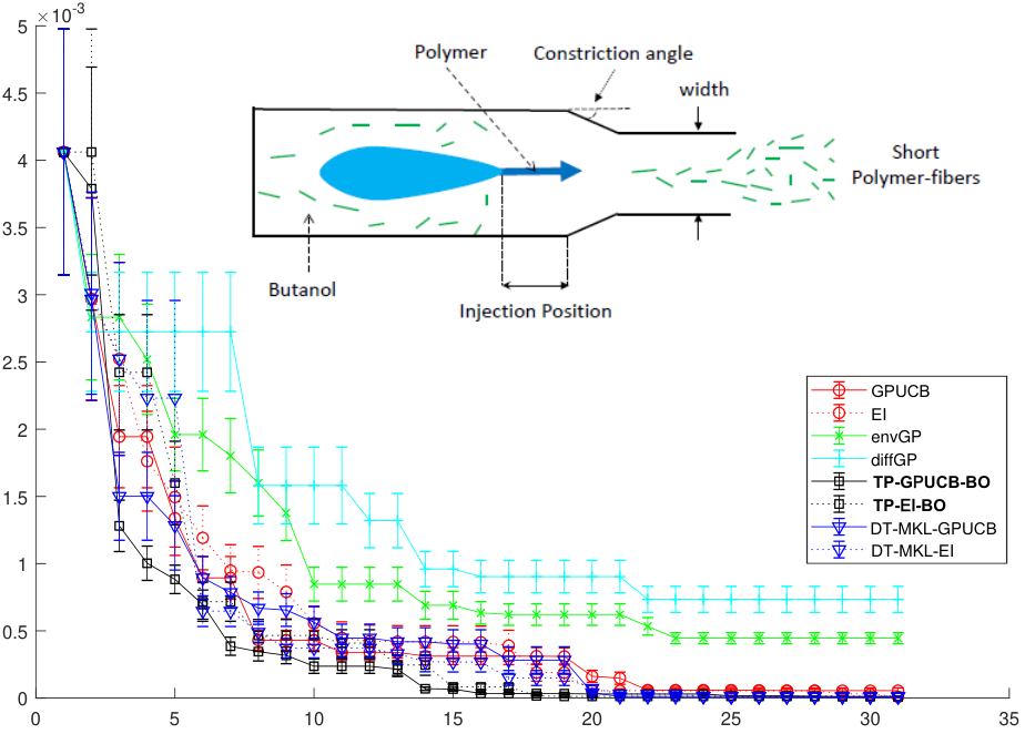
In this experiment we have tested our algorithm on the real-world application of optimizing short polymer fibre (SPF) to achieve a given (median) target length [Li et al., 2017]. This process involves the injection of one polymer into another in a special device [Sutti et al., 2014]. The process is controlled by geometric parameters (channel width (mm), constriction angle (degree), device position (mm)) and flow factors (butanol speed (ml/hr), polymer concentration (cm/s)) that parametrize the experiment (figure 2). Two devices (A and B) were used. Device A is armed by a gear pump and allows for three butanol speeds (86.42, 67.90 and 43.21), device B has a lobe pump and allows butonal speed 98, 63 and 48. Our goal is to design a new short polymer fibre using Device B with median fibre length 500m, so:
- •
Target: we aim to minimize , where is the median fibre length (m) produced by device B with settings as described above. For simulation purposes this is represented by a grid of experimental observations from [Li et al., 2017].
- •
Auxiliary dataset: consists of experimental observations of device A of the form , where is the median fibre length produced by device A with [Li et al., 2017].
Results are shown in figure 2. We note that, for this experiment, neither diffGP or envGP perform well, presumably due to the dissimilarities between and (but not their covariance structure). We note that our algorithm converges more quickly than the alternatives.
7 Notes and Future Directions
In the experiments we found that our method works well provided that the auxiliary data is sufficient to characterize the covariance of the optimization problem. As counter-examples we found that test functions that vary significantly on small scales (eg. the Levi N.13 test function), and test functions with sparse, sharp features that are easily missed (eg. the Easom test function), our method did not improve convergence (see supplementary). In the first case (Levi N.13) this is due to the inability to characterize such short-scale variation from the (comparatively) small dataset , the remedy for which is increasing the size of (but see shortly). In the second case (Easom) difficulties arise due to the fact that the target is mostly flat, so is constant for all points and subsequently we find (and hence everywhere). We note that the vanishing kernel is easily detected, and moreover that all methods considered failed to make headway on this objective.
With regard to practicality, the computational cost of evaluating is , so the cost of solving is , where term 1 is the (one-off) cost of computing , term 2 is the (one-off) cost of inverting same (this is cached), and term 3 is the cost of evaluating the GP times for global optimization (calculating and matrix multiplications). We found this acceptable provided that is not too large ( appears reasonable), but for larger auxiliary datasets some form of sparsification (e.g. [Demontis et al., 2016]) will presumably be required.
Finally it is desirable to investigate the impact of weight-prior tuning on the regret bounds associated with whichever acquisition function is selected. It is unclear at present how to proceed in this direction, so this remains an open problem.
8 Conclusion
In this paper we presented an algorithm that can use auxiliary data to construct a GP covariance corresponding to a more appropriate weight prior for the objective function than is present in “standard” covariance functions. Using this, we have shown how BO may be accelerated by modeling the objective function using this covariance function. We have demonstrated our algorithm on a practical applications (short polymer fibre manufacture) and a number of test functions. Finally we have discussed the applicability of our algorithm and future research directions.
Acknowledgments
This research was partially funded by the Australian Government through the Australian Research Council (ARC). Prof Venkatesh is the recipient of an ARC Australian Laureate Fellowship (FL170100006).
References
- [Bach et al., 2004] Bach, F. R., Lanckriet, G. R. G., and Jordan, M. I. (2004). Multiple kernel learning, conic duality and the SMO algorithm. In Proceedings of the 21st International Conference on Machine Learning (ICML), Banff.
- [Bardenet et al., 2013] Bardenet, R., Brendel, M., Kégl, B., , and Sebag, M. (2013). Collaborative hyperparameter tuning. In Proceedings of the 30th International Conference on Machine Learning (ICML-13), pages 199–207.
- [Brochu et al., 2010] Brochu, E., Cora, V. M., and de Freitas, N. (2010). A tutorial on bayesian optimization of expensive cost functions, with applications to active user modeling and heirarchical reinforcement learning. eprint arXiv:1012.2599, arXiv.org.
- [Cortes and Vapnik, 1995] Cortes, C. and Vapnik, V. (1995). Support vector networks. Machine Learning, 20(3):273–297.
- [Cristianini and Shawe-Taylor, 2005] Cristianini, N. and Shawe-Taylor, J. (2005). An Introductino to Support Vector Machines and other Kernel-Based Learning Methods. Cambridge University Press, Cambridge, UK.
- [Demontis et al., 2016] Demontis, A., Melis, M., Biggio, B., Fumera, G., and Roli, F. (2016). Super-sparse learning in similarity spaces. IEEE Computational Intelligence Magazine, 11(4):36–45.
- [Der and Lee, 2007] Der, R. and Lee, D. (2007). Large-margin classification in banach spaces. In Proceedings of the JMLR Workshop and Conference 2: AISTATS2007, pages 91–98.
- [Dragomir, 2004] Dragomir, S. S. (2004). Semi-inner products and Applications. Hauppauge, New York.
- [Duan et al., 2012] Duan, L., Tsang, I. W., and Xu, D. (2012). Domain transfer multiple kernel learning. IEEE Transactions on Pattern Analysis and Machine Intelligence, 34(3):465–479.
- [Fasshauer et al., 2015] Fasshauer, G. E., Hickernell, F. J., and Ye, Q. (2015). Solving support vector machines in reproducing kernel banach spaces with positive definite functions. Applied and Computational Harmonic Analysis, 38(1):115–139.
- [Janson, 1997] Janson, S. (1997). Gaussian Hilbert Spaces. Cambridge University Press.
- [Jones et al., 1998] Jones, D. R., Schonlau, M., and Welch, W. J. (1998). Efficient global optimization of expensive black-box functions. Journal of Global optimization, 13(4):455–492.
- [Joy et al., 2016] Joy, T. T., Rana, S., Gupta, S. K., and Venkatesh, S. (2016). Flexible transfer learning framework for bayesian optimisation. In Pacific-Asia Conference on Knowledge Discovery and Data Mining, pages 102–114. Springer.
- [Kanagawa et al., 2018] Kanagawa, M., Hennig, P., Sejdinovic, D., and Sriperumbudur, B. K. (2018). Gaussian processes and kernel methods: A review on connections and equivalences. arXiv preprint arXiv:1807.02582.
- [Lanckriet et al., 2004] Lanckriet, G. R. G., Cristianini, N., Bartlett, P., Ghaoui, L. E., and Jordan, M. I. (2004). Learning the kernel matrix with semidefinite programming. Journal of Machine Learning Research, 5:27–72.
- [Li et al., 2017] Li, C., de Celis Leal, D. R., Rana, S., Gupta, S., Sutti, A., Greenhill, S., Slezak, T., Height, M., and Venkatesh, S. (2017). Rapid bayesian optimisation for synthesis of short polymer fiber materials. Scientific reports, 7(1):5683.
- [MacKay, 1998] MacKay, D. J. C. (1998). Introduction to gaussian processes. NATO ASI Series F Computer and Systems Sciences, 168.
- [Mercer, 1909] Mercer, J. (1909). Functions of positive and negative type, and their connection with the theory of integral equations. Transactions of the Royal Society of London, 209(A).
- [Micchelli et al., 2006] Micchelli, C. A., Xu, Y., and Zhang, H. (2006). Universal kernels. Journal of Machine Learning Research, 7.
- [Mockus, 2002] Mockus, J. (2002). Bayesian heuristic approach to global optimization and examples. Journal of Global Optimization, 22(1–4):191–203.
- [Pan and Yang, 2010] Pan, S. J. and Yang, Q. (2010). A survey on transfer learning. IEEE Transactions on Knowledge and Data Engineering, 22(10):1345–1359.
- [Rasmussen, 2006] Rasmussen, C. E. (2006). Gaussian processes for machine learning. MIT Press.
- [Rasmussen and Williams, 2006] Rasmussen, C. E. and Williams, C. K. I. (2006). Gaussian Processes for Machine Learning. MIT Press.
- [Salzo and Suykens, 2016] Salzo, S. and Suykens, J. A. K. (2016). Generalized support vector regression: duality and tensor-kernel representation. arXiv preprint arXiv:1603.05876.
- [Salzo et al., 2018] Salzo, S., Suykens, J. A. K., and Rosasco, L. (2018). Solving -norm regularization with tensor kernels. In Proceedings of the International Conference on Artificial Intelligence and Statistics (AISTATS) 2018.
- [Schölkopf and Smola, 2001] Schölkopf, B. and Smola, A. J. (2001). Learning with Kernels: Support Vector Machines, Regularization, Optimization, and Beyond. MIT Press, Cambridge, Massachusetts.
- [Shilton, 2020] Shilton, A. (2001–2020). SVMHeavy: SVM, machine learning and optimisation libary. https://github.com/apshsh/SVMHeavy.
- [Shilton et al., 2017] Shilton, A., Gupta, S., Rana, S., and Venkatesh, S. (2017). Regret bounds for transfer learning in bayesian optimisation. In Singh, A. and Zhu, J., editors, Proceedings of the 20th International Conference on Artificial Intelligence and Statistics, volume 54 of Proceedings of Machine Learning Research, pages 307–315, Fort Lauderdale, FL, USA. PMLR.
- [Snoek et al., 2012] Snoek, J., Larochelle, H., and Adams, R. P. (2012). Practical bayesian optimization of machine learning algorithms. In Proceedings of NIPS 2012, pages 2951–2959.
- [Srinivas et al., 2012] Srinivas, N., Krause, A., Kakade, S. M., and Seeger, M. W. (2012). Information-theoretic regret bounds for gaussian process optimization in the bandit setting. IEEE Transactions on Information Theory, 58(5):3250–3265.
- [Sriperumbudur et al., 2011] Sriperumbudur, B. K., Fukumizu, K., and Lanckrie, G. R. G. (2011). Universality, characteristic kernels and rkhs embedding of measures. Journal of Machine Learning Research, 12.
- [Steinwart and Christman, 2008] Steinwart, I. and Christman, A. (2008). Support Vector Machines. Springer.
- [Sutti et al., 2014] Sutti, A., Kirkland, M., Collins, P., and John George, R. (2014). An apparatus for producing nano-bodies: Patent WO 2014134668 A1.
- [Suykens et al., 2002] Suykens, J. A. K., Van Gestel, T., De Brabanter, J., De Moor, B., and Vandewalle, J. (2002). Least Squares Support Vector Machines. World Scientific Publishing, New Jersey.
- [Yogatama and Mann, 2014] Yogatama, D. and Mann, G. (2014). Efficient transfer learning method for automatic hyperparameter tuning. In Proceedings of the 17th International Conference on Artificial Intelligence and Statistics (AISTATS).
- [Zhang et al., 2009] Zhang, H., Xu, Y., and Zhang, J. (2009). Reproducing kernel banach spaces for machine learning. Journal of Machine Learning Research, 10:2741–2775.