Learning to Multitask
Abstract
Multitask learning has shown promising performance in many applications and many multitask models have been proposed. In order to identify an effective multitask model for a given multitask problem, we propose a learning framework called learning to multitask (L2MT). To achieve the goal, L2MT exploits historical multitask experience which is organized as a training set consists of several tuples, each of which contains a multitask problem with multiple tasks, a multitask model, and the relative test error. Based on such training set, L2MT first uses a proposed layerwise graph neural network to learn task embeddings for all the tasks in a multitask problem and then learns an estimation function to estimate the relative test error based on task embeddings and the representation of the multitask model based on a unified formulation. Given a new multitask problem, the estimation function is used to identify a suitable multitask model. Experiments on benchmark datasets show the effectiveness of the proposed L2MT framework.
1 Introduction
Multitask learning [9] aims to leverage useful information contained in multiple tasks to help improve the generalization performance of those tasks. In the past decades, many multitask models have been proposed. According to a recent survey [34], these models can be classified into two main categories: feature-based approach and parameter-based approach. The feature-based approach uses data features as the media to share knowledge among tasks and it usually learns a common feature representation for all the tasks. This approach can be further divided into two categories: shallow approach [2, 9] and deep approach [23]. Different from the feature-based approach, the parameter-based approach links different tasks by placing regularizers or Bayesian priors on model parameters to achieve knowledge transfer among tasks. This approach can be further classified into five categories: low-rank approach [1, 26], task clustering approach [16, 18], task relation learning approach [35, 32, 36, 19, 33], dirty approach [10, 17], and multi-level approach [37, 15].
Given so many multitask models, one important issue is how to choose a good model among them for a given multitask problem. One solution is to do model selection, that is, using cross validation or its variants. One limitation of this solution is that it is computationally heavy considering that each of the candidates needs to be trained for multiple times.
In this paper, we propose a framework called learning to multitask (L2MT) to solve this issue in a learning-based approach. The main idea of L2MT is to exploit the historical multitask experience to learn how to choose a suitable multitask model for a new multitask problem. To achieve that, the historical multitask experience is represented as a training set consisting of tuples each of which has three entries: a multitask problem, a multitask model, and the relative test error that equals the ratio of the average test error of the multitask model on the multitask problem over that of the single-task learning model. Based on this training set, we propose an end-to-end approach to learn the mapping from both the multitask problem and the multitask model to the relative test error, where we need to determine the representations of the multitask problem and the multitask model. First, a Layerwise Graph Neural Network (LGNN) is proposed to learn the task embedding as the representation of each task in a multitask problem and by aggregating of all the task embeddings, the task embedding matrix is used as the representation of the multitask problem. For multitask models which have a unified formulation, task covariance matrices are used as their representations since task covariance matrices play an important role and they reveal pairwise task relations. Then both representations of the multitask problem and model are encoded in an estimation function to estimate the relative test error. For a new multitask problem, we can learn the task embedding matrix via LGNN and then in order to achieve a low relative test error, we minimize the estimation function to learn the task covariance matrix as well as the entire multitask model. Experiments on benchmark datasets show the effectiveness of the proposed L2MT framework.
2 A Unified Formulation for Multitask Learning
Before presenting the L2MT framework, in this section, we give a unified formulation for multitask learning by extending that proposed in the survey [34].
Suppose that we are given a multitask problem consisting of tasks . For task , its training dataset contains data points as well as their labels , where denotes the th data point in . The learning function for task is defined as . A regularized formulation to learn task relations, which can unify several representative models [14, 13, 16, 26, 32, 35, 27, 36, 33], is formulated as
| (1) |
where , , denotes a loss function such as the cross-entropy loss and square loss, means that is positive semidefinite (PSD), denotes the trace of a square matrix, denotes the inverse or pseduoinverse of a square matrix, and are regularization hyperparameters to control the trade-off among three terms in problem (1). The first term in problem (1) measures the empirical loss. The second term is a regularizer on based on . Similar to [35], , the task covariance matrix, is used to describe the pairwise task relations. The function in problem (1) can be considered as a regularizer on to characterize its structure.
The survey [34] has shown that the models proposed in [14, 13, 16, 32, 27, 33] can be formulated as problem (1) with different ’s, where the detailed connections between these works and problem (1) are put in the supplementary material for completeness. In the following, we propose two main extensions to enrich problem (1).11 1 [19] can fit problem (1) with some modifications, which are detailed in the supplementary material.
Firstly, the Schatten norm regularization are proved to be an instance of problem (1). As its special case, the trace norm is widely used in multitask learning [26] as a regularizer to capture the low-rank structure in . Here we generalize it to the Schatten -norm denoted by for , where is just the trace norm. To see the relation between the Schatten norm regularization and problem (1), we prove the following theorem with the proof in the supplementary material.
Theorem 1
When for any given positive scalar , by defining and , problem (1) reduces to the following problem
| (2) |
When , Theorem 1 implies that problem (1) is equivalent to the trace norm regularization. Even though can be any positive scalar, problem (2) corresponds to the Schatten -norm regularization with and when .
Secondly, the squared Schatten norm regularization is proved to be an instance of problem (1) in the following theorem.
Theorem 2
By defining , which is an extended real-value function and corresponds to a constraint on , for any given positive scalar and , problem (1) is equivalent to the following problem: .
The aforementioned multitask models with different instantiations of are summarized in Table 1. Based on the above discussion, we can see that problem (1) can embrace many or even infinite multitask models as in the (squared) Schatten norm regularization can take an infinite number of values. Given a multitask problem and so many candidate models, the top priority is to choose which model to use. One solution is to try all possible models to find the best one but it is computationally heavy. In the following section, we will give our solution: Learning to Multitask.
3 Learning to Multitask
In this section, we present the proposed L2MT framework and its associated solution.
3.1 The Framework
Recall that the aim of the proposed L2MT framework shown in Figure 1 is to determine a suitable multitask model for a test multitask problem by exploiting historical multitask experience. To achieve this, as a representation of historical multitask experience, the training set of the L2MT framework consists of tuples . denotes the space of multitask problems and denotes a multitask problem. Each multitask problem consists of learning tasks each of which is associated with a training dataset, a validation dataset, and a test dataset. As we will see later, the th task in is represented as a task embedding based on its training dataset via the proposed LGNN model and by aggregating of task embeddings of all the tasks, the task embedding matrix will be treated as the representation of the multitask problem . denotes the space of multitask models and denotes a specific multitask model which is trained on the training datasets in . can be a discrete index for multitask models or a continuous representation based on model parameters. In this sequel, based on the unified formulation presented in the previous section, is represented by the task covariance matrix and hence is continuous. One reason to choose the task covariance matrix as the representation of a multitask model is that the task covariance matrix is core to problem (1) and once it has been determined, the model parameters and can easily be obtained. denotes the relative test error , where denotes the average test error of the multitask model on the test datasets of multiple tasks in and denotes the average test error of a single-task learning (STL) model which is trained on each task independently. Hence, the training process of the L2MT framework is to learn an estimation function to map from or concretely to , where , a link function, transforms to make the estimation easier and will be introduced later. Moreover, based on problem (1), we can see is a function of hyperparameters and and so is the relative test error. Here we make an assumption that is sufficient to estimate the relative test error. This assumption empirically works very well and it can simplify the design of the estimation function. Moreover, under this assumption, we do not need to find the best hyperparameters for each training tuple, which can save a lot of computational cost.
In the test process, suppose that we are given a testing multitask problem which is not in the training set. Each task in also has a training dataset, a validation dataset and a test dataset. To obtain the relative test error as low as possible, we resort to minimizing with respect to to find the optimal task covariance matrix , where denotes the task embedding matrix for the test multitask problem and is a parameter in the link function to control its monotonic property, and then by incorporating into problem (1) without manually specifying , we can learn optimal and which are used to make prediction on the test datasets.
There are some related learning paradigms to the L2MT framework, including multitask learning, transfer learning [25], and lifelong learning [12]. However, there exist significant differences between the L2MT framework and these related paradigms. In multitask learning, the training set contains only one multitask problem, i.e., , and its goal is to learn model parameters given a multitask model. The difference between transfer learning and L2MT is similar to that between multitask learning and L2MT. Lifelong learning can be viewed as online transfer/multitask learning and hence it is different from L2MT.
3.2 Task Embedding
In order to learn the estimation function in the training process, the first thing we need to do is to determine the representation of multitask problems . Usually each multitask problem is associated with multiple training datasets each of which corresponds to a task. So we can reduce representing a multitask problem to representing the training dataset of a task, which is called the task embedding, in the multitask problem. In the following, we propose a method to represent the task embedding based on neural networks with powerful capacities.
For the ease of presentation, the training dataset of a task in a multitask problem consists of data-label pairs by omitting the task index, where is assumed to have a vectorized representation. Due to varying nature of training datasets in different tasks (e.g., the size and the relations among training data points), it is difficult to use conventional neural networks such as convolutional neural networks (CNN) or recurrent neural networks (RNN) to represent a dataset. For a dataset, usually we can represent it as a graph where each vertex corresponds to a data point and the edge between vertices implies the relation between the corresponding data points. Based on the graph representation, we propose the LGNN to obtain the task embedding. Specifically, the input to the LGNN is a data matrix . By using ReLU as the activation function, the output of the first hidden layer in LGNN is
| (3) |
where denotes the dimension of hidden representations, and denote the transformation matrix and bias, and denotes a vector or matrix of all ones with the size depending on the context. According to Eq. (3), contains the hidden representations for all the training data points in this task. With an adjacency matrix to model the relations between each pair of training data points, the output of the th hidden layer () in the LGNN is defined as
| (4) |
where and are the transformation matrix and bias, and denotes the total number of hidden layers. According to Eq. (4), the hidden representations of all the data points at the th layer (i.e., ) rely on those in the previous layer (i.e., ) and if and are correlated according to (i.e., ), their hidden representations are correlated. The term in Eq. (4) not only preserves the comprehensive information encoded in original representations but also alleviates the gradient vanishing issue by achieving the skip connection as in the highway network [30] when is large. The task embedding of this task, as a result, takes the average of the last hidden layer over all data points, i.e., . One advantage of the mean function used here is that it can handle datasets with varying sizes. In LGNN, and are learnable parameters based on the objective function presented in the next section.
The graph plays an important role in LGNN. Here we use the label information in the training dataset to construct it. For example, when each learning task is a classification problem, , the th entry in , is defined as , where denotes the set of indices of data points belonging to the nearest neighbors of . Based on the definition of and Eq. (4), when two data points are in the same class, their hidden representations have positive effects to each other. When two data points are in different classes and they are nearby (i.e., in the neighborhood), their hidden representations have negative effects to each other.
The original graph neural network [28] needs to solve the fixed point of a recursive equation, which restricts the functional form of the activation function. Graph convolutional neural networks [8, 24, 4] focus on how to select neighbored data points to do the convolution operation, while LGNN aggregates all the neighborhood information in a layerwise manner.
Given a multitask problem consisting of tasks, we construct a LGNN for all tasks with the shared parameters. Therefore, the task embedding matrix , where denotes the task embedding for the th task, is treated as the representation for the entire multitask problem. In the next section, we show how to learn the estimation function based on such representation.
3.3 Training Process
Recall that the training set in L2MT contains tuples . Applying the LGNN in the previous section, we represent with tasks as a task embedding matrix . Based on the unified formulation in Section 2, is represented by the task covariance matrix . In the training process, we aim to learn an estimation function mapping from both the task embedding matrix and the task covariance matrix to the relative test error, i.e., for , where is defined as a link function to transform the output. Considering the difficulty of designing a numerically stable to meet all positive ’s, we introduce the link function, , which transforms to real scalars being positive or negative. Different ’s may have variable scales as they are produced by different multitask models with different ’s. To make their scales comparable, we impose a restriction that equals 1. If some does not satisfy this requirement, we simply preprocess it via . Note that different ’s can have different sizes as is not fixed. By taking this into consideration, we design an estimation function, whose parameters are independent of , as
| (5) |
where is the th column in , is an matrix with its th entry equal to , and contains four real parameters to be optimized in the estimation function. In the right-hand side of Eq. (5), and are linear and RBF kernel matrices to define task similarities based on task embeddings. The first two terms in define the consistency between kernel matrices and with and controlling the positive/negative magnitude to estimate . The resultant kernel matrices with the same size as are also the key to empower the estimation function to accommodate ’s of different sizes.
The link function takes the following form: , where denotes the hyperbolic tangent function to transform a positive to the range and contains two learnable parameters.
The objective function in the training process is formulated as
| (6) |
where denotes the set of parameters to be optimized. Here we use the absolute loss as it is robust to outliers. Problem (6) indicates that the proposed method is end-to-end from the training datasets of a multitask problem to its relative test error. We optimize problem (6) via the Adam optimizer in the tensorflow package. In each batch, we randomly choose a tuple (e.g., the th tuple) and optimize problem (6) by replacing the first term with as an approximation. The left part of Figure 1 illustrates the training process.
3.4 Test Process
In the test process, suppose that we are given a new test multitask problem consisting of tasks each of which is associated with a training dataset, a validation dataset and a test dataset. The goal here is to learn the optimal automatically via the estimation function and the training datasets without manually specifying the form of in problem (1). With injected, the validation datasets in all tasks can be used to fintune the regularization hyperparameter in problem (1) and the test datasets are used to evaluate the performance of L2MT as usual.
For the training datasets in the tasks, we first apply the learned LGNN in the training process to obtain their task embedding matrix . Here the task covariance matrix is unknown and what we need to do is to estimate the task covariance matrix by minimizing the relative test error, which, however, is difficult to measure based on the training datasets. Recall that the estimation function is an approximation of the transformed relative test error by the link function. So we resort to optimize the estimation function instead. Due to the monotonically increasing property of the hyperbolic tangent function used in the link function , minimizing the relative test error via the estimation function is equivalent to minimizing/maximizing the estimation function when is positive/negative,22 2 We do not consider a trivial case that where the estimation function is to approximate a constant. leading to the minimization of with respect to , which based on Eq. (5) can be simplified as
| (7) |
where , denotes the th column in , is an matrix with its th entry equal to , and . The constraints in problem (7) are due to the requirement that the trace of the PSD task covariance matrix equals 1 as preprocessed in the training stage. It is easy to find that problem (7) is convex when and otherwise non-convex. Even though the convex/non-convex nature of problem (7) varies with , we can always find its efficient solutions summarized in the following theorem.
Theorem 3
Define the eigendecomposition of as where denotes the diagonal eigenvalue matrix with (), denotes the eigenvector matrix, and the multiplicity of is assumed to be (). When , the optimal solution of problem (7) is in the convex hull of . When , optimal solutions of problem (7) are in a set . When , the optimal solution is where is the solution of the following problem
| (8) |
According to Theorem 3, we need to solve problem (8) when . Based on the Lagrange multiplier method, we design an efficient algorithm with complexity in the supplementary material. After learning according to Theorem 3, we can plug into problem (1) and learn the optimal and for the tasks involved in the test multitask problem. The right part of Figure 1 illustrates the testing process.
3.5 Analysis
The training process of L2MT induces a novel learning problem where several multitask problem as meta-samples are used to predict the relative test errors and the task embedding matrices acts meta features to describe all the multitask problems. Hence in this section, we study the generalization bound for this novel learning problem.
For the ease of presentation, we assume each multitask problem consists of the same number of tasks. By following [7], tasks originate from a common environment that is by definition a probability measure on a learning task. In L2MT, the absolute loss is used and here we generalize to a general case where the loss function is assumed to be 1-Lipschitz in the first argument.33 3 Different Lipschitz constants can be absorbed in the scaling of the learning functions and different ranges than can be handled by a simple scaling of our results. In the test process, we can see that the task covariance matrix is a function of the task embedding matrix. Inspired by this observation, we make an assumption that there exists some function to represent the task covariance matrix in terms of the task embedding matrix. Based on such assumption, the estimation function is denoted by . Then the expected loss is defined as where the expectation is on the space of multitask problems and relative test errors, and denotes the task embedding matrix induced by the corresponding multitask problem. The training loss is defined as . Based on the Gaussian average [6, 20], we can bound in terms of as follows.
Theorem 4
Let be a real-valued function class on the space of task embeddings, the members of have values in and denote the space of transformation functions in LGNN. With probability greater than , for any and any , we have
where are universal constants, functions in are assumed to have a Lipschitz constant at most , denotes the Gaussian average where denotes a generic vector or matrix of independent standard normal variables, is assumed to be 0 by following [21], and .
According to Theorem 4, we can see that the expected loss can be upper-bounded by the sum of the training loss, the model complexity based on the task embedding matrices and a confidence term with the rate of convergence . The Gaussian average on the task embedding matrices induced by LGNN can be estimated via the chain rule [20].
4 Experiments
Four datasets are used in the experiments, including the MIT-Indoor-Scene, Caltech256, 20newsgroup, and RCV1 datasets. The MIT-Indoor-67 and Caltech256 datasets are for image classification, while the 20newsgroup and RCV1 datasets are for text classification. For these two image datasets, we use the FC8 layer of the VGG-19 network [29] pretrained on the ImageNet dataset as the feature extractor. The two text datasets are represented using “bag-of-words”, thereby lying in high-dimensional spaces. To reduce the heavy computational cost induced, we preprocess these two datasets to reduce the dimension to 1,000 by following [31] which utilizes ridge regression to select important features. The RCV1 dataset is highly imbalanced as the number of data points per class varies from 5 to 130,426. To reduce the effect of imbalanced classes to multitask learning, we keep the categories whose numbers of data samples are between 400 and 5,000. The statistics for the four datasets are recorded in Table 2.
| Dataset | # instances | # classes | # instances per class |
|---|---|---|---|
| MIT-Indoor-Scene | 15620 | 67 | [99,734] |
| Caltech256 | 29781 | 256 | [61,800] |
| 20newsgroup | 18774 | 20 | [627,997] |
| RCV1 | 36423 | 21 | [400,5000] |
Based on each dataset aforementioned, we construct the training set for L2MT in the following two steps. 1) We first construct a multitask problem in which each task is a binary classification task, which is a typical setting in multitask learning. The total number of tasks is uniformly distributed between 4 and 8 as the number of tasks in real applications is limited. For a multitask problem with tasks, we just randomly sample pairs of classes along with their data where each task is to distinguish between each pair of classes. 2) we sample multi-task problems to constitute the final training set for L2MT. The test set for L2MT can be obtained similarly and its construction is exclusively different from the training set.
Baseline methods in the comparison are a single-task learner (STL), which is trained on each task independently by adopting the cross-entropy loss, and all the instantiation models of problem (1), including regularized multitask learning (RMTL) [14], Schatten norm regularization with (SNR1) which is the trace norm regularization [26], Schatten norm regularization with (SNR2) which is equivalent to the Schatten -norm regularization according to Theorem 1, the MTRL method [35, 36], squared Schatten norm regularization with (SSNR2) which is equivalent to squared Schatten -norm regularization according to Theorem 2, clustered multitask learning (CMTL) [16], multitask learning with graphical Lasso (glMTL) [32, 27], asymmetric multitask learning (AMTL) [19], and SPATS [33]. So in total there are 10 baseline methods. Moreover, to ensure fairness of comparison, we also allow each baseline method to access and include all training datasets of all training multitask problems, besides the training datasets in a testing multitask problem at hand. Consequently, we report the better performance of each baseline method when it learns on the testing multitask problem only and on all the training and testing multitask problems, respectively.
Usually collecting a training set with many multitask problems needs to take much time and in the experiments, we only collect 100 multitask problems for training where 30% data in each task form the training dataset. For better training on such training set and controlling the model complexity, different ’s and ’s () are constrained to be identical in Eq. (4), i.e., and . There are 50 testing multitask problems in the test set.
Each entry in is initialized to be normally distributed with zero mean and variance of , and the biases are initialized to be zero. The vector of parameters in the estimation function is initialized to and in the link function is initialized to . The learning rate linearly decays from 0.01 with respect to the number of epoches.


To investigate the effect of the size of the training dataset on the performance, we vary the size of training data from 30% to 50% at an interval of 10% with the validation proportion fixed to 30% in the test process and plot the average relative test errors of different methods over STL in Figure 2, where denotes the average test error of a multitask model over all the tasks in all the test multitask problems, has a similar definition for STL, and the average relative test error is defined as . All the relative test errors of STL are equal to 1, and the performance of RMTL is not very good as its assumption that all the tasks are equally similar to each other is usually violated in real applications. Hence we omit these two methods in Figure 2 for clear presentation. According to Figure 2, we can see that some multitask models perform worse than STL with relative test errors larger than 1, which can be explained by the mismatch between data and model assumptions imposed on the task covariance. By learning the task covariance directly from data without explicit assumptions, the proposed L2MT performs better than all the baseline methods under different settings, which demonstrates the effectiveness of L2MT.

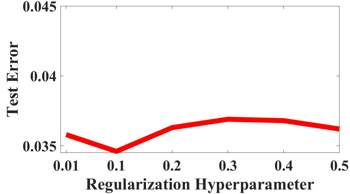


In Figure 3, we conduct the sensitivity analysis on the 20newsgroup dataset with respect to hyperparameters in L2MT, including the number of layers , the regularization hyperparameter , latent dimension and the number of neighbors in LGNN, to see their effects on the performance. According to Figure 3(a), we can see that the performance under and is better than that of , which demonstrates the usefulness of the graph information used in LGNN to learn the task embeddings. Yet the performance degrades when increases further with one reason that L2MT is likely to overfit given a small number of training tuples. As implied by Figures 3(b) and 3(d), when is in and in , the performance is not so sensitive that the choices are easier and hence in experiments we always set and to and . According to Figure 3(c), when is not very large, the performance is better than that corresponding to a larger where the overfitting is likely to occur. Based on such observation, is set to be 50. Moreover, in Figure 3(e) we test the performance of L2MT by varying , the size of training multitask problems. According to the results, the test error of L2MT decreases when is increasing, which matches the generalization bound in Theorem 4.
In previous experiments, the VGG-19 network is used as the feature extractor. It is worth noting that L2MT can even be used to update the VGG-19 network. On the Caltech256 and MIT-Indoor-Scene datasets, we use problem (6) as the objective function to fine-tune parameters in the FC layers of the VGG-19 network. After fine-tuning, the average test errors of L2MT are reduced by about 5% compared to L2MT without fine-tuning, which demonstrates the effectiveness of L2MT on not only improving the performance of multitask problems but also learning good features.
We also study other formulations for the estimation and link functions. For example, another choice for the estimation function is where with parameters and , and that for the link function is , where denotes the logarithm function with base . Compared with the estimation and link functions proposed in Section 3.3, these new functions lead to slightly worse performance (about 2% relative increase on the test error), which demonstrates the effectiveness of the proposed functions.
To assess the quality of the learned task covariance matrices by different models, we conduct a case study by constructing a multitask problem consisting of three tasks from the Caltech256 dataset. The first task is to classify between classes ‘Bat’ and ‘Clutter’, the second one is to distinguish between classes ‘Bear’ and ‘Clutter’, and the last task does classification between classes ‘Dog’ and ‘Clutter’. The learned task correlation matrices, which can be computed from task covariance matrices , by SNR1, MTRL and L2MT are , , and . From the three task correlation matrices, we can see that the correlations between the first and second tasks are close to 0 in the three models, which matches the intuition that bats and bears are almost irrelevant as they belong to different species. The same observation holds for the first and third tasks. The difference among the three methods lies in the correlations between the second and third tasks. Specifically, in SNR1 and MTRL, those correlations are close to 0, indicating that these two tasks are nearly uncorrelated, and hence the knowledge shared among the three tasks is very limited for SNR1 and MTRL. On the contrary, in L2MT, the second and third tasks have a highly negative correlation and hence there is strong knowledge leverage between those two tasks, which may be one reason that L2MT outperforms SNR1 and MTRL.
5 Conclusions
In this paper, we propose L2MT to identify a good multitask model for a multitask problem based on previous multitask problems. To achieve this, we propose an end-to-end procedure, which employs the LGNN to learn task embedding matrices for multitask problems and then uses the estimation function to approximate the relative test error. In the test process, given a new multitask problem, minimizing the estimation function leads to the identification of the task covariance matrix. As revealed in the survey [34], there is another representative formulation for the feature-based approach [2, 3, 11] in multitask learning. In our future research, we will extend the proposed L2MT method to learn good feature covariances for multitask problems based on this formulation. Moreover, the proposed L2MT method can be extended to meta learning where LGNN can be used to learn hidden representations for datasets.
References
- [1] R. K. Ando and T. Zhang. A framework for learning predictive structures from multiple tasks and unlabeled data. Journal of Machine Learning Research, 6:1817–1853, 2005.
- [2] A. Argyriou, T. Evgeniou, and M. Pontil. Multi-task feature learning. In Advances in Neural Information Processing Systems 19, pages 41–48, 2006.
- [3] A. Argyriou, C. A. Micchelli, M. Pontil, and Y. Ying. A spectral regularization framework for multi-task structure learning. In Advances in Neural Information Processing Systems 20, pages 25–32, 2007.
- [4] J. Atwood and D. Towsley. Diffusion-convolutional neural networks. In Advances in Neural Information Processing Systems 29, pages 1993–2001, 2016.
- [5] O. Banerjee, L. El Ghaoui, A. d’Aspremont, and G. Natsoulis. Convex optimization techniques for fitting sparse Gaussian graphical models. In Proceedings of the Twenty-Third International Conference on Machine Learning, pages 89–96, 2006.
- [6] P. L. Bartlett and S. Mendelson. Rademacher and Gaussian complexities: Risk bounds and structural results. Journal of Machine Learning Research, 3:463–482, 2002.
- [7] J. Baxter. A model of inductive bias learning. Journal of Artifical Intelligence Research, 12:149–198, 2000.
- [8] J. Bruna, W. Zaremba, A. Szlam, and Y. LeCun. Spectral networks and locally connected networks on graphs. CoRR, abs/1312.6203, 2013.
- [9] R. Caruana. Multitask learning. Machine Learning, 28(1):41–75, 1997.
- [10] J. Chen, J. Liu, and J. Ye. Learning incoherent sparse and low-rank patterns from multiple tasks. In Proceedings of the 16th ACM SIGKDD International Conference on Knowledge Discovery and Data Mining, pages 1179–1188, 2010.
- [11] J. Chen, L. Tang, J. Liu, and J. Ye. A convex formulation for learning shared structures from multiple tasks. In Proceedings of the 26th International Conference on Machine Learning, pages 137–144, 2009.
- [12] Z. Chen and B. Liu. Lifelong Machine Learning. Morgan & Claypool, 2016.
- [13] T. Evgeniou, C. A. Micchelli, and M. Pontil. Learning multiple tasks with kernel methods. Journal of Machine Learning Research, 6:615–637, 2005.
- [14] T. Evgeniou and M. Pontil. Regularized multi-task learning. In Proceedings of the Tenth ACM SIGKDD International Conference on Knowledge Discovery and Data Mining, pages 109–117, 2004.
- [15] L. Han and Y. Zhang. Learning tree structure in multi-task learning. In Proceedings of the 21st ACM SIGKDD Conference on Knowledge Discovery and Data Mining, 2015.
- [16] L. Jacob, F. Bach, and J.-P. Vert. Clustered multi-task learning: A convex formulation. In Advances in Neural Information Processing Systems 21, pages 745–752, 2008.
- [17] A. Jalali, P. D. Ravikumar, S. Sanghavi, and C. Ruan. A dirty model for multi-task learning. In Advances in Neural Information Processing Systems 23, pages 964–972, 2010.
- [18] A. Kumar and H. Daumé III. Learning task grouping and overlap in multi-task learning. In Proceedings of the 29 th International Conference on Machine Learning, 2012.
- [19] G. Lee, E. Yang, and S. J. Hwang. Asymmetric multi-task learning based on task relatedness and loss. In Proceedings of the 33rd International Conference on Machine Learning, pages 230–238, 2016.
- [20] A. Maurer. A chain rule for the expected suprema of Gaussian processes. In Proceedings of the 25th International Conference on Algorithmic Learning Theory, pages 245–259, 2014.
- [21] A. Maurer, M. Pontil, and B. Romera-Paredes. The benefit of multitask representation learning. Journal of Machine Learning Research, 17:1–32, 2016.
- [22] C. A. Micchelli and M. Pontil. Learning the kernel function via regularization. Journal of Machine Learning Research, 6:1099–1125, 2005.
- [23] I. Misra, A. Shrivastava, A. Gupta, and M. Hebert. Cross-stitch networks for multi-task learning. In Proceedings of IEEE Conference on Computer Vision and Pattern Recognition, pages 3994–4003, 2016.
- [24] M. Niepert, M. Ahmed, and K. Kutzkov. Learning convolutional neural networks for graphs. In Proceedings of the 33nd International Conference on Machine Learning, pages 2014–2023, 2016.
- [25] S. J. Pan and Q. Yang. A survey on transfer learning. IEEE Transactions on Knowledge and Data Engineering, 22(10):1345–1359, 2010.
- [26] T. K. Pong, P. Tseng, S. Ji, and J. Ye. Trace norm regularization: Reformulations, algorithms, and multi-task learning. SIAM Journal on Optimization, 20(6):3465–3489, 2010.
- [27] P. Rai, A. Kumar, and H. Daume. Simultaneously leveraging output and task structures for multiple-output regression. In Advances in Neural Information Processing Systems 25, pages 3185–3193, 2012.
- [28] F. Scarselli, M. Gori, A. C. Tsoi, M. Hagenbuchner, and G. Monfardini. The graph neural network model. IEEE Transactions on Neural Networks, 20(1):61–80, 2009.
- [29] K. Simonyan and A. Zisserman. Very deep convolutional networks for large-scale image recognition. CoRR, abs/1409.1556, 2014.
- [30] R. K. Srivastava, K. Greff, and J. Schmidhuber. Highway networks. CoRR, abs/1505.00387, 2015.
- [31] S. Yang, L. Yuan, Y.-C. Lai, X. Shen, P. Wonka, and J. Ye. Feature grouping and selection over an undirected graph. In Proceedings of ACM SIGKDD Conference on Kownledge Discovery and Data Mining, 2012.
- [32] Y. Zhang and J. G. Schneider. Learning multiple tasks with a sparse matrix-normal penalty. In Advances in Neural Information Processing Systems 23, pages 2550–2558, 2010.
- [33] Y. Zhang and Q. Yang. Learning sparse task relations in multi-task learning. In Proceedings of the 31th AAAI Conference on Artificial Intelligence, 2017.
- [34] Y. Zhang and Q. Yang. A survey on multi-task learning. arXiv preprint, arXiv:1707.08114, 2017.
- [35] Y. Zhang and D.-Y. Yeung. A convex formulation for learning task relationships in multi-task learning. In Proceedings of the 26th Conference on Uncertainty in Artificial Intelligence, pages 733–742, 2010.
- [36] Y. Zhang and D.-Y. Yeung. A regularization approach to learning task relationships in multitask learning. ACM Transactions on Knowledge Discovery from Data, 8(3):article 12, 2014.
- [37] A. Zweig and D. Weinshall. Hierarchical regularization cascade for joint learning. In Proceedings of the 30th International Conference on Machine Learning, pages 37–45, 2013.
Supplementary Material for “Learning to Multitask”
Details in the Unified Formulation (1)
In [14, 13], the priori information about the similarity between a pair of tasks and denoted by is used to define a regularizer to enforce similar tasks to have similar model parameters, where denotes the norm of a vector. It is easy to see that such regularizer equals the second term of problem (1) by setting , where is the Laplacian matrix of a graph whose th entry equals . Here , an extended real-value function, acts as a constraint to constrain to be .
Jacob et al. [16] propose a clustered multitask learning method, which can be viewed as an instance of problem (1), to group all the tasks in the spirit of the -means clustering algorithm by setting as
where are additional hyperparameters and denotes an identity matrix with appropriate size.
Inspired by the graphical Lasso method [5], we consider an instance of problem (1) by setting as , where denotes the norm of a vector or matrix, the sum of the absolute values of all entries in it. This setting of encourages the inverse of to be sparse and has been investigated in [32, 27].
Zhang and Yang [33] observe that when there are a large number of tasks, it is better to learn sparse task relations. Then based on problem (1), they aim to learn a sparse , leading to an implementation of as .
In [19], is assumed to lie in the space spanned by , i.e., or equivalently , leading to a regularizer , where denote the Frobenius norm. By assuming that the linear spanning is sparse, the corresponding is formulated as
| (9) |
where denotes the norm of a vector or matrix and denotes an identity matrix with the appropriate size. In Eq. (9), we make several modifications to the original work. Firstly, different tasks are assumed to be equally important. Secondly, to capture the negative correlations between tasks, here is allowed to have negative values while in the original work is nonnegative. Thirdly, diagonal entries in can be zero via the regularization to avoid a trivial solution where equals .
The aforementioned multitask models with the corresponding are summarized in Table 1.
Proof for Theorem 1
Proof. By setting the derivative of problem (1) with respect to to be zero, we can obtain the solution for as
By plugging this solution into problem (1), we can get an equivalent problem as
By defining the singular value decomposition (SVD) of as where is the rank of , denotes the set of orthogonal matrices with size , , , and is a diagonal matrix containing the singular values of , we have
in which we reach the conclusion.
Proof for Theorem 2
Proof. The regularizer is defined as
Since
where the inequality holds due to the von Neumann’s trace inequality, then we can get
where denotes the th singular value of a matrix, the second inequality holds due to Lemma 26 in [22], and the equality holds when .
Proof for Theorem 3
Proof. When , the Lagrangian of problem (7) is defined as
where is the Lagrange multiplier corresponding to the equality constraint. Since is PSD, by setting the derivative of with respect to to zero, we can get
where the function operates on the spectral of the matrix. Based on this equation, we can see that shares eigenvectors with and by plugging this observation into problem (7), it is easy to check that the eigenvalues of satisfy problem (8).
When equals 0, based on the Lagrange multiplier method, problem (7) can be reformulated as
which is equal to the dual form as
Since the inner minimization is linear in terms of , the dual form can be simplified as
It is easy to see that the optimal solution for this dual problem is that equals the minimum eigenvalue of and . So the null space of is spanned by . Based on the KKT condition, we have which implies that is in the null space of , leading to the solution lying in the convex hull of which satisfies the equality constraint in problem (7).
When , problem (7) is non-convex and we cannot use the Lagrange multiplier method to analyze it. Since the objective function of problem (7) consists of two terms, we can decompose problem (7) into two subproblems:
| (10) |
and
| (11) |
If these two subproblems have some common solution, then this solution will also be the solution to problem (7). Problem (11) is just problem (7) when equals 0 and hence based on the above analysis, its optimal solutions are in the convex hull of . As , problem (10) is equivalent to the following problem
which can be reformulated as
| (12) |
where denotes the th eigenvalue of and . The equivalence holds since the trace function can be expressed in terms of eigenvalues of a PSD matrix and independent of eigenvectors. For problem (12), we have
where the inequality holds since is in implied by the constraints and the equality holds due to the equality constraint in problem (12). So the optimal value for problem (12) is 1, which is achieved when only one entry in equals 1 while others are 0. It is easy to check that some optimal solutions of problem (11), including , satisfied this condition, making them optimal solutions of problem (7).
Algorithm for Solving Problem (8)
Obviously problem (8) is a quadratic program (QP) problem. Many off-the-shelf solvers such as CVX could be used to solve it in polynomial time. To achieve further speedup, we propose a more efficient solution by exploiting the special structure of this problem. Note that the only variable coupling in problem (8) comes from the equality constraint. The Lagrangian corresponding to this constraint is given by
Setting the derivative of with respect to to 0, we can see that the minimum is reached when . Since each is required to be nonnegative and is a quadratic function of , the optimal solution for is given by
| (13) |
Plugging the optimal solution of into , we can obtain the dual problem as
| (14) |
Obviously, the objective function of problem (14) is a piecewise linear or quadratic function over regions determined by the sequences . The main idea of our method is to determine the functional form of problem (14) over each region, then compute the local optimum over each region which has an analytical solution, and finally obtain the global optimum by comparing all the local optima. So the main problem is to determine the coefficients of problem (14) over each region efficiently.
When , the objective function of problem (14) is , where , , and , and it has an analytical solution as . When , problem (14) has no well-defined solution since the objective function becomes . So we only need to consider the situation where . We summarize the algorithm for solving problem (14) in Algorithm 1. This algorithm needs to scan the sequence at most twice which costs . So the complexity of the whole algorithm is which is much more efficient than existing QP solvers.
Proof for Theorem 4
Proof. According to [6], we have
where . By the Lipschitz property of the loss function and Corollary 11 in [21], we have where . Note that is defined by . According to Theorem 2 in [20], we have
where are universal constants, denotes the diameter among and equals the longest distance between any two entries. It is easy to show that based on the triangular inequality in the Euclidean distance metric. Since equals 0, by setting and , we reach the conclusion.