PCA by Optimisation of Symmetric Functions
has no Spurious Local Optima

Let $A\in\mathbb{R}^{m\times n}$ be a data matrix, with rows corresponding to $m$ different data vectors, and columns corresponding to $n$ different features. Successful dimensionality reduction is at the heart of classification, regression, and other learning tasks that often suffer from the “curse of dimensionality”, where having a small number of training samples in relation to the data dimension (namely, $m\ll n$) typically leads to overfitting [1].

To reduce the dimension of data from $n$ to $p\leq n$, consider a matrix $X$ with orthonormal columns. Then the rows of $AX\in\mathbb{R}^{m\times p}$ correspond to the data vectors (namely, the rows of $A$) projected onto the column span of $X$, which we denote by $\mathrm{range}(X)$. In particular, the new data matrix $AX$ has reduced dimension $p$, while the number $m$ of projected data vectors is unchanged, see Figure 1. Principal Component Analysis (PCA) is one of the oldest dimensionality reduction techniques that can be traced back to the work of Pearson [2] and Hotelling [3], motivated by the observation that often data lives near a lower-dimensional subspace of $\mathbb{R}^{n}$, see Figure 2. PCA identifies this subspace by finding a suitable matrix $X$ that retains in $AX$ as much as possible of the energy of $A$, and the optimal $X$ is called the loading matrix. The columns of the loading matrix also reveal the hidden correlations between different features by identifying groups of variables that occur with jointly positive or jointly negative weights, for example in gene expression data [4].

PCA is also the building block of other dimensionality reduction techniques such as sparse PCA [5], kernel PCA [6, 7], multi-dimensional scaling [8], and Nonnegative Matrix Factorisation (NMF) [9]. For example, sparse PCA aims to find the important features of data by requiring the loading matrix to be sparse, namely, to have very few nonzero entries. Sparse PCA is useful for instance in studying gene expression data, where we are interested in singling out a small number of genes that are responsible for a certain trait or disease [10]. NMF, on the other hand, requires both $AX$ and $X$ to have nonnegative entries, which is valuable in recommender systems for instance where the data matrix $A$ containing, say, film ratings is nonnegative and one would expect the same from the projected data matrix $AX$.

More formally, assume throughout this paper that the data matrix $A\in\mathbb{R}^{m\times n}$ is mean-centred. That is, $\sum_{i=1}^{m}a_{i}=0$, where $a_{i}\in\mathbb{R}^{n}$ is the $i$-th row of $A$, namely, the $i$-th data vector. For $p\leq n$, let $\mathbb{R}^{n\times p}_{p}$ be the space of full-rank $n\times p$ matrices and consider the trace inflation function

	$\displaystyle f_{\operatorname{tr}}:\mathbb{R}^{n\times p}_{p}$	$\displaystyle\rightarrow$	$\displaystyle\mathbb{R}$
	$\displaystyle X$	$\displaystyle\mapsto$	$\displaystyle\frac{\|AX\|_{F}^{2}}{\|X\|_{F}^{2}}=\frac{\operatorname{tr}(X^{*}A^{*}AX)}{\operatorname{tr}(X^{*}X)},$		(1)

and the program

$$\arg\max\left\{f_{\operatorname{tr}}(X):\;X\in\mathrm{St}(n,p)\right\}.$$

(2)

Above, $\|\cdot\|_{F}$ and $\mbox{tr}(\cdot)$ return the Frobenius norm and trace of a matrix, respectively, and $A^{*}$ is the transpose of matrix $A$. With $p\leq n$, $\mathrm{St}(n,p)$ above denotes the the Stiefel manifold, the set of all $n\times p$ matrices with orthonormal columns. Note that when $X\in\mathrm{St}(n,p)$, the denominator in the definition of $f_{\operatorname{tr}}(X)$ in (1) is constant, but we include this term to highlight the structural similarity with other inflation functions that we will study later.

It is a consequence of the celebrated Eckart-Young-Mirsky (EYM) Theorem that a Stiefel matrix $X\in\mathrm{St}(n,p)$ is a global maximiser of Program (2) if and only if it consists of $p$ leading right singular vectors of $A$, namely, the right singular vectors of $A$ corresponding to its $p$ largest singular values [11, 12]. In other words, Program (2) performs PCA on the data matrix $A$: The loading matrix, namely, global maximiser of Program (2), is a $p$-leading right singular factor $V_{p}\in\mathbb{R}^{n\times p}$ of $A$, and the projected data matrix $AV_{p}\in\mathbb{R}^{n\times p}$ contains the first $p$ principal components of $A$.

Note also that Program (2) is non-convex because $\mathrm{St}(n,p)\subset\mathbb{R}^{n\times p}$ is a non-convex set. Even though non-convex, Program (2) behaves like a convex problem in the sense that any local maximiser of Program (2) is also a global maximiser. Indeed, it is also a consequence of the EYM Theorem that Program (2) does not have any spurious local maximisers. Moreover, all saddle points of this program are strict, namely, have an ascent direction. Therefore the non-convex Program (2) can be efficiently solved (to global optimality) using (certain variants of) the stochastic gradient descent, see for instance [13, 14, 15]. Even more efficiently, solving Program (2) or equivalently computing the loading matrix and the principal components of $A$ can be done in $O(\max(m,n)p^{2})$ operations using fast algorithms for Singular Value Decomposition (SVD), see for example Algorithm 8.6.1 in [16].

In analogy to $f_{\operatorname{tr}}$ in (1), let us define the volume inflation function by

	$\displaystyle f_{\det}:\mathbb{R}^{n\times p}_{p}$	$\displaystyle\rightarrow$	$\displaystyle\mathbb{R}$
	$\displaystyle X$	$\displaystyle\mapsto$	$\displaystyle\frac{\det(X^{*}A^{*}AX)}{\det(X^{*}X)},$		(3)

where $\det$ stands for determinant and, in analogy to Program (2), consider the program

$$\arg\max\left\{f_{\det}(X):\;X\in\mathrm{St}(n,p)\right\}.$$

(4)

Observe that Programs (2) and (4) coincide for $p=1$, namely, when we seek the leading principal component of the matrix $A$, in which case $X^{*}A^{*}AX$ and $X^{*}X$ are both positive scalars. Unlike $f_{\operatorname{tr}}$, note that $f_{\det}$ is invariant under an arbitrary change of basis. Indeed, for arbitrary $X\in\mathbb{R}^{n\times p}_{p}$ and $\Theta\in\mathrm{GL}(p)$, we have that

	$\displaystyle f_{\det}(X\Theta)$	$\displaystyle=\frac{\det(\Theta)^{2}\det(X^{*}A^{*}AX)}{\det(\Theta)^{2}\det(X^{*}X)}$
		$\displaystyle=f_{\det}(X),$		(5)

where $\mathrm{GL}(p)$ is the general linear group, the set of all invertible $p\times p$ matrices. That is, $f_{\det}$ is naturally defined on the Grassmannian $\mathrm{Gr}(n,p)$ and consequently Program (4) is equivalent to the program

$$\arg\max\left\{f_{\det}(X):\;X\in\mathbb{R}^{n\times p}_{p}\right\}.$$

(6)

Because $f_{\det}$ is invariant under any change of basis by (5), Program (6) inherently constitutes an optimization over the Grassmannian $\mathrm{Gr}(n,p)$. Moreover, it is important that Program (6) is effectively unconstrained because $\mathbb{R}^{n\times p}_{p}$ is an open subset of $\mathbb{R}^{n\times p}$ with nonempty interior. To summarise, the drawback of Program (2) in Section 1 which served as the motivation of this work is overcome by Program (6), because it is an unconstrained optimisation program that involves an objective function defined naturally on the Grassmannian.

A key observation of this paper is that Program (6) appears to be a good model for dimensionality reduction. Indeed, note that $X^{*}A^{*}AX\in\mathbb{R}^{p\times p}$ is the sample covariance matrix of the projected data $AX$. Consider the normal distribution $\mathcal{N}(0,X^{*}A^{*}AX)$ with zero mean and covariance matrix $X^{*}A^{*}AX$, which has ellipsoidal level sets of the form

$$\{z\in\mathbb{R}^{p}\,:\,z^{*}X^{*}A^{*}AXz=c\},$$

(7)

for arbitrary $c\geq 0$. Let $B_{c}$ be the bounding box of this level set and note that the volume of $B_{c}$ is $c^{p}\sqrt{\det(X^{*}A^{*}AX)}$. We can therefore interpret Program (6) as maximising the volume of this bounding box. That is, Program (6) loosely-speaking finds the directions that maximise the volume of the projected dataset.

In contrast, Program (2) maximises the energy of the projected data. That is, Program (2) maximises the diameter of the above bounding box, namely, $c\sqrt{\mbox{tr}(X^{*}A^{*}AX)}$, rather than its volume, see Figure 3. It is perhaps peculiar that $\mbox{tr}(X^{*}A^{*}AX)$ is commonly referred to as the “total variance” of the dataset, for this quantity does not play any role in the normalising constant of the normal distribution $\mathcal{N}(0,X^{*}A^{*}AX)$, whereas $\det(X^{*}A^{*}AX)$ does, in direct generalization of the role the variance plays in the one-dimensional case.

At any rate, we see that Programs (2,6) are both sensible approaches for linear dimensionality reduction, but that their geometric justifications are very different. Somewhat surprisingly, we find that Program (6) also performs PCA of $A$ and has no spurious local optima, exactly like Program (2). The next result is proven in Section 5.

The main contribution of Theorem 1 is its Part ii) about the global landscape of the objective function $f_{\det}$, stating that the non-convex Program (6) behaves like a convex problem in the sense that any local maximiser (minimiser) of Program (6) is also a global maximiser (minimiser). Moreover, saddle points of Program (6) are strict. In this way too, the two Programs (2,6) are similar, see Section 1. Note that Part ii) of Theorem 1 is crucial in the design of new dimensionality reduction algorithms: The instability of all stationary points except the global optima and the strictness of all saddle points establishes that, for example, stochastic gradient ascent, converges to the correct solution in polynomial time [13, 14]. That is, the non-convex Program (6) can be efficiently solved to global optimality. However, as discussed in Section 1, computationally efficient algorithms for PCA are already available and application of, say, stochastic gradient ascent to Program (6) is not intended to replace those algorithms. Instead, as discussed in Section 3, the unconstrained Program (6) potentially opens up a radically new approach to structured PCA.

We remark that Theorem 1 is in line with a recent trend in computational sciences to understand the geometry and performance of non-convex programs and algorithms [22, 15, 23, 24, 25, 26, 27, 28, 29, 30, 31, 32, 33]. While the available results do not apply to our problem, the underlying phenomena are closely related. Perhaps the closest result to our work is [28], stating that the (non-convex) matrix completion program has no spurious local optima when given access to randomly-observed matrix entries. This result in a sense extends the EYM Theorem [11, 12] to partially-observed matrices.

From a computational perspective, we may consider the program

$$\arg\max\left\{\log(f_{\det}(X)):\;X\in\mathbb{R}^{n\times p}_{p}\right\},$$

(9)

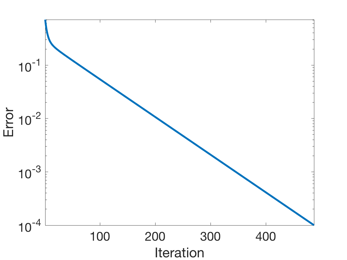
which is equivalent to Program (6) but has better numerical stability. As a numerical example, we generated generic $U,V\in\mathrm{Orth}(100)$ and random matrix $A\in\mathbb{R}^{100\times 100}$ with SVD $A=U\Sigma V^{*}$. The singular values of $A$, namely the entries of the diagonal matrix $\Sigma\in\mathbb{R}^{100\times 100}$, were selected according to the power law. To be specific, we took $\sigma_{i}=i^{-1}$ to generate Figure 4 and $\sigma_{i}=i^{-2}$ to generate Figure 5, for every $i\in[100]=\{1,2,\cdots,100\}$. For $p=5$, we let $V_{p}\in\mathbb{R}^{n\times p}$ denote the first $p$ columns of $V$ and, by Theorem 1, the unique maximiser of Programs (6,9). (Note that $V_{p}$ is also the unique maximiser of Program (2) by the EYM Theorem.) In order to find $V_{p}$, we then applied gradient ascent to Program (9) with fixed step size of $\rho=5$ and random initialisation, producing a sequence of estimates $\{X_{l}\}_{l}\subset\mathbb{R}^{n\times p}$. We also recorded the error $\|X_{l}{X}_{l}^{\dagger}-V_{p}V_{p}^{*}\|$ in the $l$th iteration, namely the sine of the principal angle between $\mathrm{range}(X_{l})$ and $\mathrm{range}(V_{p})$, which is plotted in Figures 4 and 5. As predicted by Theorem 1, the error vanishes in both examples as the algorithm progresses. We also refer the interested reader to [34] for a comparison between Programs (2,9), as well as LAPACK’s implementation of Lanczos’ method [16] for performing PCA. While the numerical results presented in [34] are encouraging, a more comprehensive study is required to investigate the competitiveness of Program (9) for PCA, as an alternative to more mainstream approaches [16].

It might also be helpful to highlight the following practical consideration. Let $\widetilde{X}\in\mathbb{R}^{n\times p}$ denote a maximiser of Programs (6) or (9). Given $\widetilde{X}$, a few extra steps are required to compute the complete SVD of $A$, which we now list. Let $\widehat{X}\in\mathbb{R}^{n\times p}$ be an orthonormal basis for $\widetilde{X}$, which can be computed in $O(np^{2})$ operations by SVD. Then computing the SVD of $A\widehat{X}=\widehat{U}\widehat{\Sigma}\widehat{V}^{*}$ can be performed in merely $O(mp^{2})$ operations and yields the diagonal coefficients of $\widehat{\Sigma}$ as the $p$ leading singular values of $A$, as well as $\widehat{U}$ and $\widehat{X}\widehat{V}$ as the corresponding $p$ leading left and right singular vectors of $A$, respectively.

As we will see in this section, the unconstrained formulation of PCA in Program (6) might be of particular interest in practice, in contrast to Program (2) which is restricted to the Stiefel manifold. Indeed, the determinant formulation of PCA in Program (6) might allow for a more elegant approach to structured PCA, in which we wish to impose additional structure on the loading matrix, such as sparsity or nonnegativity.

For the purposes of this brief and informal discussion, let us focus on sparse PCA, the problem of finding a small number of features that best describe the data matrix $A\in\mathbb{R}^{m\times n}$. As one application, when working with gene expression data, we are interested in a small number of features (genes) which are responsible for certain traits or diseases [35, 36]. The “dual” of sparse PCA can also be interpreted as data clustering.

Loosely speaking, sparse PCA is the problem of finding a sparse¹¹ 1 A sparse matrix has a small number of nonzero entries. matrix $X\in\mathbb{R}^{n\times p}$ that retains, in the projected data $AX\in\mathbb{R}^{m\times p}$, as much as possible of the energy of $A$. More formally, sparse PCA might be formulated as a natural generalisation of Program (2), namely,

$$\arg\max\left\{f_{\operatorname{tr}}(X):\;X\in\mathrm{St}(n,p)\mbox{ and }\|X\|_{0}\leq k\right\},$$

(10)

where $\|X\|_{0}$ is the number of nonzero entries of $X$, and the typically small integer $k$ is the sparsity level. Note that Program (10) forces $X$ to have orthonormal columns and few nonzero entries, which tends to be restrictive and is also a somewhat questionable objective in the first place. With a few exceptions, particularly [5], this problem is often addressed by deflating $A$, namely, finding the sparse principal components sequentially, that is, one by one. Indeed, note that the Stiefel constraint from Program (10) is redundant when $p=1$, namely, when $X$ is a column vector. One could therefore find the leading sparse principal component of $A$, say $\widetilde{x}_{1}\in\mathbb{R}^{n}$, by solving Program (10) with $p=1$, remove its contribution from $A$ by forming $A_{1}=A-A\widetilde{x}_{1}\widetilde{x}_{1}^{*}$, and then solve Program (10) with $A_{1}$ in place of $A$ to find the second sparse principal component $\widetilde{x}_{2}\in\mathbb{R}^{n}$, and so on [37]. However, deflating $A$ is believed to be inherently problematic when the problem is ill-posed [5].

The determinant formulation of PCA in Program (9) might provide an elegant alternative to Program (10). Recall that the feasible set of Program (9) is an open subset of $\mathbb{R}^{n\times p}$ with nonempty interior, and thus Program (9) is effectively unconstrained. We can therefore formulate sparse PCA by imposing a sparsity constraint on Program (9), namely,

$$\arg\max\left\{\log(f_{\det}(X)):\;X\in\mathbb{R}^{n\times p}_{p}\mbox{ and }\|X\|_{0}\leq k\right\},$$

(11)

which requires $X$ to be full-rank and sparse, relaxing the far more restrictive requirement of being Stiefel and sparse in Program (2). Note that removing the full-rank requirement in Program (11) is impossible as that would mean $A$ has fewer than $p$ principal components and therefore the problem is ill-defined.

Similar ideas might be applied to nonnegative matrix factorisation, in which $X$ and $AX$ are both required to be nonnegative. More generally, the unconstrained nature of Program (9) might provide an entirely new approach to many structured dimensionality reduction problems, a research direction that remains to be explored in the future. In particular, what is the global geometry of Program (11)? What is the precise relationship between Programs (10) and (11)?

So far, we have seen that maximising the trace objective function in Program (2) and maximising the determinant objective function in Program (6) are equivalent, and both provide the leading principal components of the data matrix $A$. Moreover, both non-convex programs can be solved to global optimality efficiently, see the discussion after Theorem 1 for example. Indeed, these claims for Program (2) follow from the EYM Theorem [11, 12] and the claims for Program (6) follow from Theorem 1, see Sections 1 and 2.

Note that both $\mbox{tr}(X^{*}A^{*}AX)$ and $\det(X^{*}A^{*}AX)$ are elementary symmetric polynomials, namely, both are coefficients of the characteristic polynomial of $X^{*}A^{*}AX$. More specifically, let $X^{*}A^{*}AX=W_{X}\operatorname{diag}(\lambda_{X})W_{X}^{*}$ be the eigen-decomposition of $X^{*}A^{*}AX$, where $W_{X}\in\mathrm{Orth}(p)$ is an orthonormal matrix and the vector $\lambda_{X}\in\mathbb{R}^{p}$ contains the eigenvalues of $X^{*}A^{*}AX$. Here, $\operatorname{diag}(\lambda_{X})\in\mathbb{R}^{p\times p}$ is the diagonal matrix formed by the vector $\lambda_{X}$. Then the characteristic polynomial associated with $X^{*}A^{*}AX$ takes $t\in\mathbb{R}$ to

	$\displaystyle\det(\operatorname{I}_{p}+tX^{*}A^{*}AX)$	$\displaystyle=\det(W_{X}(\operatorname{I}_{p}+t\operatorname{diag}(\lambda_{X}))W_{X}^{*})\qquad\left(W_{X}\in\mathrm{Orth}(p)\right)$
		$\displaystyle=\det(W_{X})\cdot\det(\operatorname{I}_{p}+t\operatorname{diag}(\lambda_{X}))\cdot\det(W_{X}^{*})$
		$\displaystyle=\det\left[\begin{array}[]{cccc}1+t\cdot\lambda_{X,1}&0&\cdots&0\\ 0&1+t\cdot\lambda_{X,2}&\cdots&0\\ \vdots&\vdots&\ddots&\\ 0&0&\cdots&1+t\cdot\lambda_{X,p}\end{array}\right]\qquad\left(\det(W_{X})=1\right)$
		$\displaystyle=\prod_{i=1}^{p}(1+t\cdot\lambda_{X,i})$
		$\displaystyle=:\sum_{q=0}^{p}s_{q}(X^{*}A^{*}AX)\cdot t^{q},$		(16)

where the $q$th elementary symmetric polynomial $s_{q}:\mathrm{Sym}(p)\rightarrow\mathbb{R}$ is the coefficient of $t^{q}$ above, namely,

	$\displaystyle s_{q}:\mathrm{Sym}(p)$	$\displaystyle\rightarrow$	$\displaystyle\mathbb{R}$
	$\displaystyle B$	$\displaystyle\mapsto$	$\displaystyle\sum_{1\leq i_{1}<\cdots<i_{q}\leq p}\,\prod_{j=1}^{q}\lambda_{B,i_{j}},$		(17)

with the convention that $s_{0}(B)=1$. Above, $\{\lambda_{B,i}\}_{i=1}^{p}$ are the eigenvalues of $B\in\mathrm{Sym}(p)$, and $\mathrm{Sym}(p)$ denotes the set of symmetric $p\times p$ matrices over the real numbers. We also remark that elementary symmetric polynomials are spectral functions in that they only depend on the eigenvalues of the input matrix. As mentioned earlier, $\operatorname{tr}(X^{*}A^{*}AX)=s_{1}(X^{*}A^{*}AX)$ and $\det(X^{*}A^{*}AX)=s_{p}(X^{*}A^{*}AX)$.

In analogy to trace and determinant objective functions (1,3), let us define

	$\displaystyle f_{s_{q}}:\mathbb{R}^{n\times p}$	$\displaystyle\rightarrow$	$\displaystyle\mathbb{R}$
	$\displaystyle X$	$\displaystyle\mapsto$	$\displaystyle\frac{s_{q}(X^{*}A^{*}AX)}{s_{q}(X^{*}X)},$		(18)

for every $q\in[p]:=\{1,\dots,p\}$. In particular, $f_{s_{1}}=f_{\operatorname{tr}}$ in (1) and $f_{s_{p}}=f_{\det}$ in (3) are two special cases. Lastly, in analogy to Programs (2,4), consider the program

$$\arg\max\left\{f_{s_{q}}(X):\;X\in\mathrm{St}(n,p)\right\}.$$

(19)

Again note that Programs (2) and (4) are special cases of Program (19) for $q=1$ and $q=p$, respectively. Revisiting the geometric interpretation discussed in Section 2, we may also verify that ${f_{s_{q}}(X)}$ is proportional to the sum of volumes squared of all $q$-dimensional facets of the bounding box $B_{c}$, see right after (7) and also Figure 3. In this sense, Program (19) finds the projected data $AX$ that maximises this geometric attribute.

Generalising the EYM Theorem for Program (2) and Theorem 1 for Program (4), the following result states that Program (19) performs PCA of $A$ and has no spurious local optima for every $q\in[p]$, see Section 6 for the proof.

We first begin with a change of variables. Let $A=U\Sigma V^{*}$ be the SVD of $A$, where $U\in\mathbb{R}^{m\times m}$ and $V\in\mathbb{R}^{n\times n}$ are orthonormal matrices, and the diagonal matrix $\Sigma\in\mathbb{R}^{m\times n}$ is formed by the singular values of $A$ in nonincreasing order, denoted by $\sigma_{1}\geq\sigma_{2}\geq\cdots$. Let us set $\Gamma:=\Sigma^{*}\Sigma\in\mathbb{R}^{n\times n}$ for short and note that

$$\Gamma=\mbox{diag}(\gamma),\qquad\mbox{where }\gamma=\left[\begin{array}[]{ccccc}\sigma_{1}^{2}&\cdots&\sigma_{r}^{2}&0&\cdots\end{array}\right]^{*}\in\mathbb{R}^{n},$$

(25)

where $\mbox{diag}(\gamma)$ shapes the vector $\gamma$ into a diagonal matrix, and $r=\mbox{rank}(A)$ is the rank of $A$, namely, the number of positive singular values of $A$. Under the change of variables from $X$ to $Y=V^{*}X$, Program (6) is equivalent to

$$\arg\max\left\{\frac{\det(Y^{*}\Gamma Y)}{\det(Y^{*}Y)}\,:\,Y\in\mathbb{R}^{n\times p}_{p}\right\}.$$

(26)

Without loss of generality, we will therefore assume that $A^{*}A=\Gamma$ in (3), namely, we henceforth set

$$f_{\det}(X)=\frac{\det(X^{*}\Gamma X)}{\det(X^{*}X)}.$$

(27)

We will prove Theorem 1 by studying the stationary points of Program (6). This program is unconstrained and therefore a stationary point $X_{s}\in\mathbb{R}^{n\times p}_{p}$ of Program (6) is characterised by $\nabla f_{\det}(X_{s})=0$. In light of the invariance in (5), we can also assume without loss of generality that $X_{s}\in\operatorname{St}(n,p)$. A stationary point $X_{s}\in\operatorname{St}(n,p)$ of Program (6) thus satisfies

$$\nabla f_{\det}(X_{s})=2\Gamma X_{s}\nabla\det(X_{s}^{*}\Gamma X_{s})-2\det(X_{s}^{*}\Gamma X_{s})\cdot X_{s}\nabla\det(X_{s}^{*}X_{s})=0.$$

(28)

Note that the determinant is a spectral function, namely, it only depends on the eigenvalues of its input matrix. More precisely, for a matrix $Z\in\mathbb{R}^{p\times p}$, it holds that

$$\det(Z)=e_{p}(\lambda_{Z}):=\prod_{i=1}^{p}\lambda_{Z,i},$$

(29)

where $\lambda_{Z,i}$ is the $i$-th eigenvalue of $Z$ and the vector $\lambda_{Z}=[\lambda_{Z,1},\cdots,\lambda_{Z,p}]$ contains the eigenvalues of $Z$. The derivative of a spectral function is well-known. To be specific, let $Z=W_{Z}\cdot\text{diag}(\lambda_{Z})\cdot W_{Z}^{*}$ be the eigen-decomposition of $Z$, where $W_{Z}\in\mathrm{Orth}(p)$ is an orthonormal matrix and, as before, $\text{diag}(\lambda_{Z})\in\mathbb{R}^{p\times p}$ is the diagonal matrix formed by the vector $\lambda_{Z}$. For a spectral function $\phi:\mathrm{Sym}(p)\rightarrow\mathbb{R}$, there exists a symmetric function $\psi:\mathbb{R}^{p}\rightarrow\mathbb{R}$ such that

$$\phi(Z)=\phi(\text{diag}(\lambda_{Z}))=\psi(\lambda_{z}),$$

(30)

where we recall that a symmetric function is a function that remains invariant after changing the order of its arguments. We then have from [38] that

$$\nabla\phi(Z)=W_{Z}\cdot\mbox{diag}(\nabla\psi(\lambda_{Z}))\cdot W_{Z}^{*}.$$

(31)

In our case, with $\phi=e_{p}$ and when $Z\in\mathrm{GL}(p)$, namely, when $Z$ is non-singular, we have that

	$\displaystyle\nabla\det(Z)$	$\displaystyle=W_{Z}\cdot\text{diag}(\nabla e_{p}(\lambda_{Z}))\cdot W_{Z}^{*}\qquad\text{(see \eqref{eq:grad of spec})}$
		$\displaystyle=W_{Z}\cdot\text{diag}\left(e_{p}(\lambda_{Z})\left[\begin{array}[]{ccc}\frac{1}{\lambda_{Z,1}}&\cdots&\frac{1}{\lambda_{Z,p}}\end{array}\right]^{*}\right)\cdot W_{Z}^{*}\qquad\text{(see \eqref{eq:def of ep})}$
		$\displaystyle=\det(Z)W_{Z}\cdot\text{diag}\left(\left[\begin{array}[]{ccc}\frac{1}{\lambda_{Z,1}}&\cdots&\frac{1}{\lambda_{Z,p}}\end{array}\right]^{*}\right)\cdot W_{Z}^{*}.\qquad\text{(see \eqref{eq:def of ep})}$

Returning to the proof and recalling that $X_{s}\in\operatorname{St}(n,p)$, (5) allows us to write that

$\displaystyle\nabla\det(X_{s}^{*}X_{s})=I_{p}.$

(34)

Likewise, after recalling that $X_{s}^{*}\Gamma X_{s}\in\mathrm{GL}(p)$ by assumption, it follows from (5) that

$\displaystyle\nabla\det(X_{s}^{*}\Gamma X_{s})=\det(X_{s}^{*}\Gamma X_{s})\cdot(X_{s}^{*}\Gamma X_{s})^{-1}.$

(35)

Substituting (34,35), we find that (28) holds if and only if $\Gamma X_{s}=X_{s}X_{s}^{*}\Gamma X_{s}$, and since $X_{s}X_{s}^{*}$ is the projection into $\mathrm{range}(X_{s})$, this is true if and only if $\mathrm{range}(\Gamma X_{s})\subseteq\mathrm{range}(X_{s})$. From this it follows that $X_{s}\in\operatorname{St}(n,p)$ such that $X_{s}^{*}\Gamma X_{s}\in\mathrm{GL}(p)$ is a stationary point of Program (6), if and only if

$$\mathrm{range}(X_{s})=\mathrm{range}(\Gamma X_{s}).$$

(36)

The following result, proved in Appendix A, characterises the stationary points of Program (6). That is, the next result characterises matrices $X_{s}\in\mathrm{St}(n,p)$ that satisfy (36).

References

- [1] T. Hastie, R. Tibshirani, and J. Friedman. The Elements of Statistical Learning: Data Mining, Inference, and Prediction. Springer Series in Statistics. Springer New York, 2013.
- [2] K. Pearson. On lines and planes of closest fit to systems of points in space. Philosophical Magazine, 2(11):559–572, 1901.
- [3] H. Hotelling. Relations between two sets of variates. Biometrika, (28):321–377, 1936.
- [4] Orly Alter and Gene Golub. Singular value decomposition of genome-scale mrna lengths distribution reveals asymmetry in rna gel electrophoresis band broadening. PNAS, 103(32):11828–11833, 2006.
- [5] Michel Journée, Yurii Nesterov, Peter Richtárik, and Rodolphe Sepulchre. Generalized power method for sparse principal component analysis. Journal of Machine Learning Research, 11(Feb):517–553, 2010.
- [6] B. Schölkopf and A.J. Smola. Learning with Kernels: Support Vector Machines, Regularization, Optimization, and Beyond. Adaptive computation and machine learning. MIT Press, 2002.
- [7] J. Shawe-Taylor and N. Cristianini. Kernel Methods for Pattern Analysis. Cambridge University Press, 2004.
- [8] I. Borg and P. Groenen. Modern Multidimensional Scaling: Theory and Applications. Springer Series in Statistics. Springer New York, 2013.
- [9] Nicolas Gillis. The why and how of nonnegative matrix factorization. Regularization, Optimization, Kernels, and Support Vector Machines, 12(257), 2014.
- [10] Orly Alter, Patrick O Brown, and David Botstein. Singular value decomposition for genome-wide expression data processing and modeling. Proceedings of the National Academy of Sciences, 97(18):10101–10106, 2000.
- [11] C. Eckart and G. Young. The approximation of one matrix by another of lower rank. Psychometrika, 1:211–218, 1936.
- [12] L. Mirsky. Symmetric gauge functions and unitarily invariant norms. Quart. J. Math. Oxford, pages 1156–1159, 1966.
- [13] Chi Jin, Rong Ge, Praneeth Netrapalli, Sham M Kakade, and Michael I Jordan. How to escape saddle points efficiently. In Proceedings of the 34th International Conference on Machine Learning-Volume 70, pages 1724–1732. JMLR. org, 2017.
- [14] Aryan Mokhtari, Asuman Ozdaglar, and Ali Jadbabaie. Escaping saddle points in constrained optimization. In Advances in Neural Information Processing Systems, pages 3633–3643, 2018.
- [15] Ju Sun, Qing Qu, and John Wright. When are nonconvex problems not scary? arXiv preprint arXiv:1510.06096, 2015.
- [16] G.H. Golub and C.F. Van Loan. Matrix Computations. Johns Hopkins Studies in the Mathematical Sciences. Johns Hopkins University Press, 1996.
- [17] R.A. Horn, R.A. Horn, and C.R. Johnson. Matrix Analysis. Cambridge University Press, 1990.
- [18] National Institute of Standards, Technology (U.S.), and International SEMATECH. NIST/SEMATECH Engineering Statistics Handbook. 2002.
- [19] A. Hyvarinen, J. Karhunen, and E. Oja. Independent Component Analysis. Adaptive and Cognitive Dynamic Systems: Signal Processing, Learning, Communications and Control. Wiley, 2004.
- [20] R.A. Horn and C.R. Johnson. Topics in Matrix Analysis. Cambridge University Press, 1994.
- [21] Samuel Karlin and Yosef Rinott. A generalized cauchy binet formula and applications to total positivity and majorization. Journal of multivariate analysis, 27(1):284–299, 1988.
- [22] Q. Li and G. Tang. The nonconvex geometry of low-rank matrix optimizations with general objective functions. arXiv:1611.03060v1 [cs.IT], 2016.
- [23] Armin Eftekhari, Laura Balzano, Dehui Yang, and Michael B Wakin. Snipe for memory-limited pca from incomplete data. arXiv preprint arXiv:1612.00904, 2016.
- [24] Samuel Burer and Renato DC Monteiro. A nonlinear programming algorithm for solving semidefinite programs via low-rank factorization. Mathematical Programming, 95(2):329–357, 2003.
- [25] Nicolas Boumal, Vlad Voroninski, and Afonso Bandeira. The non-convex Burer-Monteiro approach works on smooth semidefinite programs. In Advances in Neural Information Processing Systems, pages 2757–2765, 2016.
- [26] Srinadh Bhojanapalli, Anastasios Kyrillidis, and Sujay Sanghavi. Dropping convexity for faster semi-definite optimization. In Conference on Learning Theory, pages 530–582, 2016.
- [27] Srinadh Bhojanapalli, Behnam Neyshabur, and Nati Srebro. Global optimality of local search for low rank matrix recovery. In Advances in Neural Information Processing Systems, pages 3873–3881, 2016.
- [28] Rong Ge, Jason D Lee, and Tengyu Ma. Matrix completion has no spurious local minimum. In Advances in Neural Information Processing Systems, pages 2973–2981, 2016.
- [29] Chi Jin, Sham M Kakade, and Praneeth Netrapalli. Provable efficient online matrix completion via non-convex stochastic gradient descent. In Advances in Neural Information Processing Systems, pages 4520–4528, 2016.
- [30] Mahdi Soltanolkotabi, Adel Javanmard, and Jason D Lee. Theoretical insights into the optimization landscape of over-parameterized shallow neural networks. arXiv preprint arXiv:1707.04926, 2017.
- [31] Rong Ge, Jason D Lee, and Tengyu Ma. Learning one-hidden-layer neural networks with landscape design. arXiv preprint arXiv:1711.00501, 2017.
- [32] Rong Ge, Furong Huang, Chi Jin, and Yang Yuan. Escaping from saddle points—online stochastic gradient for tensor decomposition. In Conference on Learning Theory, pages 797–842, 2015.
- [33] Rong Ge and Tengyu Ma. On the optimization landscape of tensor decompositions. In Advances in Neural Information Processing Systems, pages 3653–3663, 2017.
- [34] Raphael A Hauser, Armin Eftekhari, and Heinrich F Matzinger. Pca by determinant optimisation has no spurious local optima. In Proceedings of the 24th ACM SIGKDD International Conference on Knowledge Discovery & Data Mining, pages 1504–1511. ACM, 2018.
- [35] Iain M Johnstone and Arthur Yu Lu. On consistency and sparsity for principal components analysis in high dimensions. Journal of the American Statistical Association, 104(486):682–693, 2009.
- [36] Yash Deshpande and Andrea Montanari. Information-theoretically optimal sparse pca. In Information Theory (ISIT), 2014 IEEE International Symposium on, pages 2197–2201. IEEE, 2014.
- [37] Alexandre d’Aspremont, Laurent E Ghaoui, Michael I Jordan, and Gert R Lanckriet. A direct formulation for sparse pca using semidefinite programming. In Advances in neural information processing systems, pages 41–48, 2005.
- [38] Adrian S Lewis and Hristo S Sendov. Quadratic expansions of spectral functions. Linear algebra and its applications, 340(1-3):97–121, 2002.
- [39] Alan Edelman, Tomás A Arias, and Steven T Smith. The geometry of algorithms with orthogonality constraints. SIAM journal on Matrix Analysis and Applications, 20(2):303–353, 1998.