Region-Based Classification of PolSAR Data Using Radial Basis Kernel Functions With Stochastic Distances
Abstract
Region-based classification of PolSAR data can be effectively performed by seeking for the assignment that minimizes a distance between prototypes and segments. Silva et al. (2013) used stochastic distances between complex multivariate Wishart models which, differently from other measures, are computationally tractable. In this work we assess the robustness of such approach with respect to errors in the training stage, and propose an extension that alleviates such problems. We introduce robustness in the process by incorporating a combination of radial basis kernel functions and stochastic distances with Support Vector Machines (SVM). We consider several stochastic distances between Wishart: Bhatacharyya, Kullback-Leibler, Chi-Square, Rényi, and Hellinger. We perform two case studies with PolSAR images, both simulated and from actual sensors, and different classification scenarios to compare the performance of Minimum Distance and SVM classification frameworks. With this, we model the situation of imperfect training samples. We show that SVM with the proposed kernel functions achieves better performance with respect to Minimum Distance, at the expense of more computational resources and the need of parameter tuning. Code and data are provided for reproducibility.
keywords
PolSAR; image classification; stochastic distance; Minimum Distance Classifier; SVMbUFAL – Universidade Federal de Alagoas, LaCCAN – Laboratório de de Computação Científica e Análise Numérica, Maceió, Brazil;
cIME – Instituto Militar de Engenharia, Seção de Ensino de Engenharia Cartográfica, Rio de Janeiro, Brazil;
dINPE – Instituto Nacional de Pesquisas Espaciais, DPI – Divisão de Processamento de Imagens, São José dos Campos, Brazil.
1 Introduction
The availability of Polarimetric Synthetic Aperture Radar (PolSAR) sensors has increased as a consequence of the technological advances in Remote Sensing. Compared to conventional SAR sensors, PolSAR is able to acquire the amplitude, phase, and orientation of the electromagnetic waves reflected from targets in different transmission and reception polarizations. The use of these images is challenging, among other reasons, because of the data structure (complex matrices in each pixel), their properties (the Gaussian additive noise is not valid), and the signal-to-noise ratio (typically very low). Bearing these characteristics in mind, several specific methods have been developed for PolSAR image processing and classification.
PolSAR image classification has been intensively investigated. The notion that more information on the same area leads to better classification is intuitive. Lee, Grunes, and Kwok (1994) and Cloude and Pottier (1997) proposed two pioneer approaches for PolSAR data classification. While the former develops a pixel-based method based on the Maximum Likelihood Classifier under the Complex Multivariate Wishart distribution, the latter is an unsupervised classification through the eigenvalue analysis of coherency matrices.
Several PolSAR data classification approaches have been proposed since then. Frery, Correia, and Freitas (2007) used specific probability density functions for PolSAR intensity data in the classic Maximum Likelihood Classifier method. Ersahin, Cumming, and Ward (2010) based their approach for segmentation and classification of PolSAR data on spectral graph partitioning. Du et al. (2014) used a Kernel Extreme Learning Machine with multiple polarimetric and spatial features. Tao et al. (2015) proposed a feature extraction method based on Independent Component Analysis and tensor decomposition. Recently, Hou et al. (2017) proposed a semi-supervised method able to learn even when the training data quality and quantity are both poor.
Silva et al. (2013) investigated the use of stochastic distances between Complex Multivariate Wishart distributions on a region-based approach. The performance of using the Kullback-Leibler, Bhattacharyya, Hellinger, Rényi, and Chi-Square stochastic distances was assessed, providing evidence that such leads to better results when compared to the Maximum Likelihood Classifier using the Complex Multivariate Wishart distribution for pixel-based PolSAR classification as proposed in Lee, Grunes, and Kwok (1994). Furthermore, the Kullback-Leibler, Bhattacharyya, and Rényi distances are more indicated than Hellinger and Chi-Square. Ratha, Bhattacharya, and Frery (2018) proposed projecting PolSAR data onto Kennaugh matrices, and then computing the geodesic distance between elementary targets and the observed information.
Negri, Silva, and Mendes (2016) presented a new version of K-Means algorithm for region-based classification of PolSAR data by using a stochastic distance between Complex Multivariate Wishart models and a hypothesis test derived from this kind of measure. Similarly, Negri et al. (2016) verified the use of Bhattacharyya distance with a Support Vector Machine (SVM) through kernel functions for region-based classification of SAR data. However, to the best of the authors’ knowledge, there is still room for investigating other distances and specific distributions for PolSAR images. Also, the influence of errors on the training data has received little attention in the literature.
This study aims at analyzing the use of a number of stochastic distances as inputs for an SVM with kernel functions for PolSAR region-based classification. Additionally, it presents comparisons with the Minimum Distance Classifier framework investigated by Silva et al. (2013). Such comparisons are conducted on PolSAR images, both simulated and from operational sensors, and different classification scenarios. Such scenarios include an analysis of the often encountered situation of using imperfect, i.e. contaminated, training samples.
The remainder of this article is organized as follows. Fundamental concepts regarding statistical PolSAR modelling, and the use of stochastic distances for region-based classification are presented in Section 2. In Section 3, these concepts are applied in two case studies. Conclusions are presented in Section 4.
2 Statistical region-based PolSAR classification
2.1 Statistical PolSAR modelling
The backscatter signal measured by a PolSAR sensor can be represented through the complex scattering vector . Each component of is a complex number that carries the amplitude and phase of a polarization combination. The polarizations are indicated by the subscripts in , where, for example, denotes the signal recorded with vertical polarization from a signal initially emitted with horizontal polarization. Considering the reciprocity of an atmospheric medium, which makes similar to , the scattering vector is simplified to (Frery, Correia, and Freitas 2007).
An -looks covariance matrix is the average of backscatter measurements in a neighborhood:
| (1) |
where and represent the conjugate and transposed operators, respectively. The diagonal elements of are nonnegative numbers that represent the intensity of the signal measured on a specific polarization.
Assuming that follows a zero-mean Complex Gaussian distribution (Goodman 1963, cf.), it is possible to obtain the distribution of , the scaled Complex Multivariate Wishart law, which is characterized by the following probability density function:
| (2) |
where .
The parameters and are the number of looks and the target mean covariance matrix. The determinant, inversion and trace operators are denoted , and , respectively.
The scaled Complex Multivariate Wishart model is valid in textureless areas. Target variability can be included by one or more additional parameters; the reader is referred to the work by Deng et al. (2017) for a comprehensive survey of models for PolSAR data.
2.2 Stochastic distances between Complex Multivariate Wishart distributions
A divergence is a measure of the difficulty of discriminating between two models. Csiszár (1967) proposed the divergence family, providing a formally organized framework to analytically obtain divergence measures between distributions. Salicru et al. (1994) proposed a more general class of divergences, the divergence, through the adoption of an additional function ().
Consider the random variables and defined on the same support with distributions characterized by the densities and , respectively, where and are parameters. The divergence between and is given by:
| (3) |
where is a convex function and is a strictly increasing function with and for all . Several well-known divergence measures can be obtained by choosing and , but they are not necessarily symmetric.
The symmetrization allows to obtain distances measures from any divergence . This leads to the following properties:
- 1.
Non-negativity: ;
- 2.
Identity (of indiscernible): ;
- 3.
Symmetry: .
Additionally, if a distance has the following property, then it is a metric:
- 4.
Triangle inequality: ,
where , and have the same support . It is noteworthy that Bathacharrya, Kullback-Leibler, Rényi, Hellinger and Chi-Square distances are not metrics since the triangle inequality is not fulfilled.
Nascimento, Cintra, and Frery (2010) computed the Bathacharrya, Kullback-Leibler, Rényi (of order ), Hellinger, Jensen-Shannon, Arithmetic-Geometric, Triangular and Harmonic Mean stochastic distances between distributions. These distances were successfully used to evaluate contrast differences among regions in intensity Synthetic Aperture Radar (SAR) images.
Frery, Nascimento, and Cintra (2014) developed analytic expressions for the first four aforementioned stochastic distances between scaled Complex Multivariate Wishart distributions. Previously, the Chi-Square stochastic distance between Complex Multivariate Wishart distributions was presented in Frery, Nascimento, and Cintra (2011). These distances were used by Silva et al. (2013) in PolSAR imagery classification by a minimum distance criterion.
Let and be two random variables modelled by scaled Complex Multivariate Wishart distributions and . The Bathacharrya, Kullback-Leibler, Rényi (order ) and Hellinger stochastic distances expressions between scaled Complex Multivariate Wishart distributions, according to Frery, Nascimento, and Cintra (2014), are given by:
| (4) | ||||
| (5) | ||||
| (6) | ||||
| (7) | ||||
| (8) |
where returns the modulus of a real number.
2.3 Region-based PolSAR image classification
Let be an image defined on the grid whose pixels are elements of the attribute space . We use the notation to represent that a pixel of has attribute . The image support can be partitioned in disjoint subsets , such that .
A region-based classification process consists of associating a class from a set of possible classes to all the pixels that comprise the region . A supervised region-based decision rule is built trough information available from a set of labeled regions . The notation indicates that is assigned to the class .
Silva et al. (2013) adopt the Minimum Distance Classifier framework using stochastic distances as a measure to compare the similarity between classes and unlabeled regions. We refer to this method as Minimum Stochastic Distance Classifier (MSDC). The pixel values in an unlabeled region are used to estimate a probability distribution. This region is then assigned to the closest class in distribution, according to an stochastic distance. The class distributions are modeled based on information from .
Formally, let be an unlabeled region and let be a stochastic distance between distributions estimated from the attributes of the pixels in and the class . An assignment is made when the following rule is satisfied:
| (9) |
In Equation (9), is estimated with all the pixels assigned to in .
Other methods can be adopted to perform region-based classification beyond the MSDC as, for instance, Support Vector Machines (SVMs). SVMs have received great attention because of their excellent generalization ability, their independence of data distribution and their robustness with respect to the Hughe’s phenomenon (Bruzzone and Persello 2009).
The use of kernel functions, , is a common strategy to improve SVM classification performance on nonlinearly separable patterns. Kernel functions also allow the application of SVMs in problems where patterns cannot be represented as vectors.
A kernel function is symmetric and conforms to the Mercer theorem conditions (Theodoridis and Koutroumbas 2008). However, as such verification may be not trivial there are alternative ways to develop such functions. For example, adopting the radial basis function model (Schölkopf and Smola 2002):
| (10) |
where is a strictly positive real function and is a metric.
Equation (10) gives a hint to develop suitable kernel functions for PolSAR region-based image classification. A sensible choice for is the negative exponential function, and , as a measure of similarity between the input data, a metric based on stochastic distances between distributions. It is noteworthy that equations (4) to (8) will not produce valid kernel functions since they do not attain the triangle inequality.
However, if D is a stochastic distance with such that for , the following expression provides a metric:
| (11) |
The identity property of stems from (11). Non-negativity and symmetry are inherited from D, which is a distance, since adding a positive constant will not invalidate such proprieties. Finally, the triangle inequality is fulfilled since the following relations are satisfied:
once we have that . The constant can be chosen as the largest distance measured by D in the classification problem. Figure 1 illustrates this procedure.
We can thus define kernel functions for PolSAR region-based image classification using the model from Equation (10), the expression from Equation (11) and considering the substitution of D by a stochastic distance given by Equations (4) to (8):
| (12) |
where is a user-adjusted parameter. We denote the kernel functions obtained from the Bathacharrya, Kullback-Leiber, Hellinger, Rényi e Chi-Square distances as , , , and , respectively.
We make clear that denotes a kernel function between estimates of distributions and computed with the observations in regions and .
3 Experiments and Results
In this section, we present studies of region-based image classification of actual and simulated PolSAR data using the stochastic distances presented in Section 2.2 by both MSDC (i.e., , , , and ) and through the kernel functions, defined in Section 2.3 (i.e., , , , and ).
The first study (Section 3.1) consists of the classification of simulated images generated with basis on parameters estimated from targets in an actual image. The second case study (Section 3.2) focuses on the classification of the PolSAR image used to extract the parameters. The results are compared by accuracy measures and hypothesis tests.
The scenarios considered in both studies allow a robustness analysis. Specifically, the results from simulated data are assessed through the overall accuracy, while the actual data are verified with the kappa coefficient of agreement (Congalton and Green 2009).
Figure 2 presents an overview of the experiment design, whereas the specifics are discussed in the following sections.
The actual PolSAR data belongs to an image acquired on 2009 March 13 by the ALOS-PALSAR sensor with approximately resolution after a multi-look process. This image, with center near to South and West, corresponds to a region near the Tapajós National Forest, State of Pará, Brazil.
A field work campaign conducted in September 2009 identified the following land use and land cover (LULC) types: Primary Forest (PF), Regeneration (RE), Pasture (PS), Bare Soil (BS), and three types of Agriculture (A1, A2 and A3). These agricultural classes differ on the crop type or growing stage. Figs. 3(a), 3(b) and 3(c) present the study area location, a color composition of the ALOS-PALSAR image and the LULCs, respectively.


The experiments run on a computer with an Intel Core i7 processor, and of RAM running the Debian Linux version 8.1 operating system. The platform was IDL (Interactive Data Language) version 7.1. The code is freely available at https://github.com/rogerionegri/SVM-PolSAR.
3.1 Classification of Simulated Data
3.1.1 Image Simulation
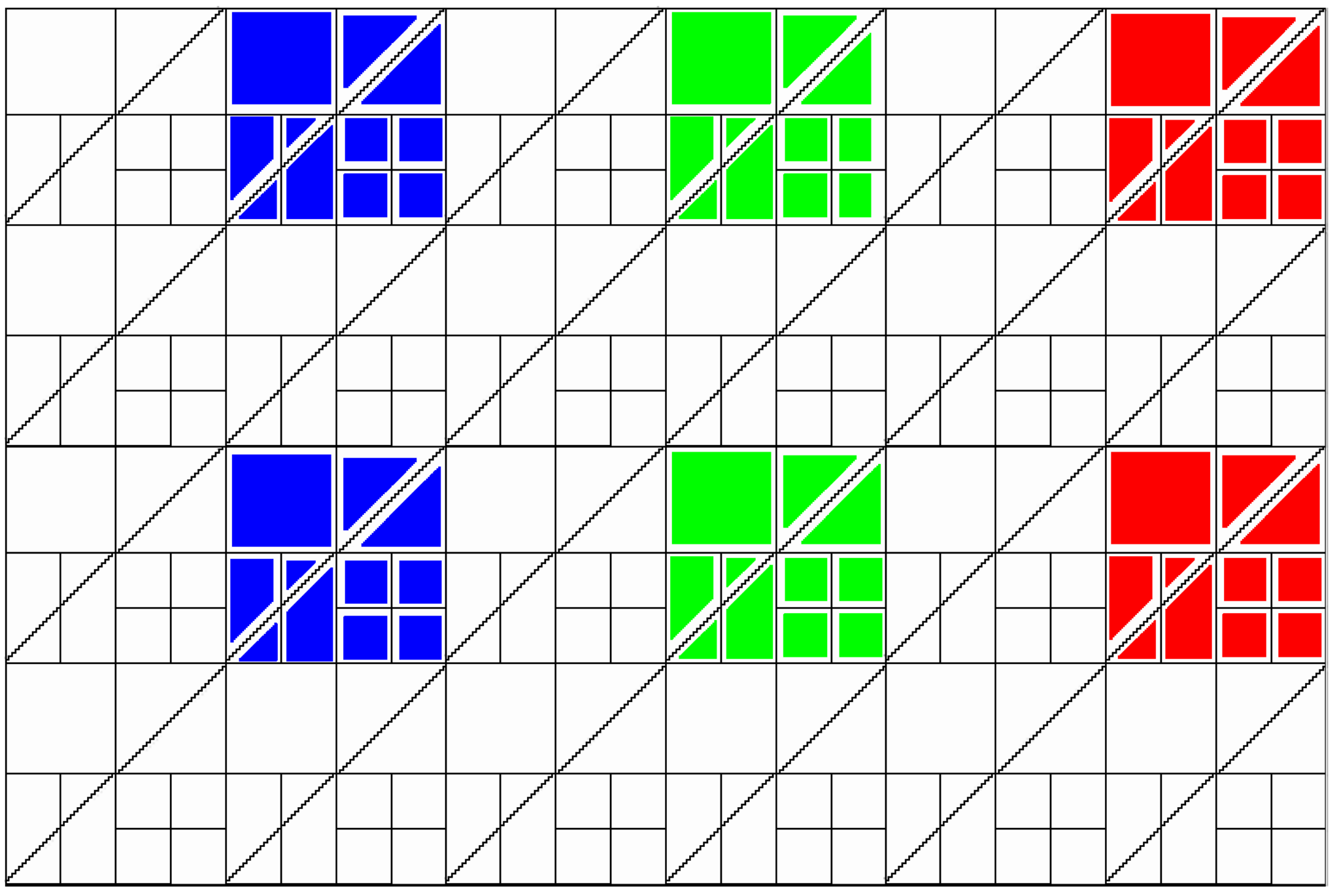
The process adopted for simulated images involves two primary steps. The first step consists of defining a “phantom image” which is an idealized model for the spatial distribution of classes. The phantom is formed by six identical blocks of pixels. Each block represents a distinct class, which is partitioned into segments of different dimension. Figure 4(a) illustrates the phantom image and the structure inside the blocks.
The second step consists of simulating pixels values. For this purpose, we adopted a procedure based on Goodman (1963). In order to obtain samples from the Wishart distribution with covariance matrix and looks, we obtain independent deviates from scattering vectors following a Complex Multivariate Gaussian distribution with zero mean and covariance matrix :
| (13) |
where i represents the imaginary unit and the covariance matrix of the Gaussian law is
We then apply Equation (1) to obtain an observation. Each class is modeled by a covariance matrix obtained by averaging observations from the corresponding LULC.
We introduce intra-class variability to describe “imperfect” samples and, with this, model plausible errors in the training stage. Frery, Ferrero, and Bustos (2009) analyzed the effect of such errors in classification, and showed that incorporating context is a way of alleviating such problem.
Consider the (true, unobserved) covariance matrix that describes a class. If it is estimated with perfect samples, i.e., with independent identically distributed observations from the hypothesized distribution, then its maximum likelihood estimate will be as close to as the information in the sample permits. Errors in the training stage may lead to suboptimal estimates in terms of bias and variance. We model this situation by introducing random perturbations in , as follows.
The user believes each class is characterized by but, in fact, the data come from slightly different models: . These models are built by adding random covariance matrices to , which is obtained estimating from actual data from a single class. Each perturbation covariance matrix is formed as
where are independent uniform random variables on , where is the diagonal element of , and controls the perturbation. With this, each mean intensity in is a value in , where is the (wrongly assumed for the whole block) mean intensity, and is the standard deviation of .
Notice that the correct model for each class would be a mixture of distributions, but the user will train each class with samples from (typically slightly) different laws; cf. the colored squares in Fig. 5(a). With this, we assess how the classification techniques perform in the practical situation of using less classes for describing a complex truth, and not collecting samples from all the underlying classes. Fig. 4(c) shows, in logarithmic scale, the intensity of averaged covariance matrices as squares, and their respective perturbed versions.
As can be seen from Fig. 4(c) we consider the following situations:
- •
Classes that do not overlap, e.g. A1 and A3, A1 and PF, A1 and RG, A3 and all others, PF and BS, PS and BS, RG and BS
- •
Classes with some overlap, e.g. A1 and PS, A1 and BS,
- •
Classes that overlap, e.g. PS and RG.
This is corroborated by (14) below, which shows the Hellinger distances between the classes.
|
(14) |
Figure 4(b) presents a simulated image, where it is possible to identify the intra-class variability. The covariance matrices that plays the rule of in the simulation process, estimated from observed LULC samples shown in Figure 3(c), are presented as Appendix.


3.1.2 Classification and Results
A set of fifty images were simulated independently following the procedure described in Section 3.1.1 Each image was then classified using the MSDC and SVM methods. MSDC used the stochastic distances between Complex Multivariate Wishart distributions by plugging Equations (4) to (8) in (9). SVM also employed these distances through the kernel functions in (11) and (12).
Furthermore, although the simulated images have six well-defined blocks of targets (regions), such objects where classified in two scenarios (i.e., classes configurations). The first scenario considers each block as a single class, the second scenario considers the blocks and ; and ; and and as three distinct classes. The second scenarios describes situations where the user specifies less classes than those actually present in the image. According to this organization, Figures 5(a) and 5(b) present the training samples and the ideal results expected for the first scenario; similarly, Figures 5(c) and 5(d) refer to the second scenario.



Using preliminary tests, the order of the Rényi distance () was set to for both SVM and MSDC methods. The SVM penalty and kernel parameter were adjusted for each image, considering a fixed parameter space, through an exhaustive search for the configuration which produces the most accurate results with respect to testing samples. In this study, penalty ranges in and the kernel flexibility in .
Two multiclass strategies were considered for SVM in order to assess relationships between strategies, scenarios, kernels and method performance: One-Against-All (OAA) and One-Against-One (OAO), denoted SVM-OAA and SVM-OAO respectively. Details about these strategies can be found in Webb and Copsey (2011).
We measured the accuracy of each classification result by the number of correctly classified regions, without taking into account training regions. Figure 6 represents the classification accuracy achieved by each method for different configurations (i.e., stochastic distances/kernel and multiclass strategy for SVM). Table 1 presents the -values of a bilateral -test to check the statistical equality between the accuracy values achieved by two distinct combinations of methods and distances. Further discussions about statistical equality are based on of confidence.
In the following tables SA, SO and MS represent the SVM-OAA, SVM-OAO and MSDC methods, and B, K, C, R and H represent the Bhattacharyya, Kullback-Leibler, Chi-Square, Rényi and Hellinger stochastic distances in the kernel functions.
| B | K | C | R | H | ||||||||||||
| SA | SO | MS | SA | SO | MS | SA | SO | MS | SA | SO | MS | SA | SO | MS | ||
| B | SA | – | .808 | .191 | .929 | .872 | .186 | .001 | .000 | .000 | .927 | .850 | .189 | .979 | .850 | .191 |
| SO | .914 | – | .147 | .757 | .936 | .142 | .001 | .000 | .000 | .752 | .957 | .145 | .797 | .966 | .147 | |
| MS | .000 | .000 | – | .228 | .162 | .984 | .002 | .000 | .000 | .224 | .156 | .987 | .203 | .161 | 1.00 | |
| K | SA | .861 | .785 | .000 | – | .815 | .224 | .001 | .000 | .000 | 1.00 | .795 | .227 | .000 | .796 | .228 |
| SO | .978 | .935 | .000 | .840 | – | .157 | .001 | .000 | .000 | .811 | .979 | .160 | .858 | .973 | .162 | |
| MS | .000 | .000 | .996 | .000 | .000 | – | .002 | .000 | .000 | .220 | .151 | .997 | .199 | .156 | .984 | |
| C | SA | .000 | .000 | .064 | .000 | .000 | .064 | – | .881 | .691 | .001 | .001 | .002 | .001 | .001 | .002 |
| SO | .000 | .000 | .355 | .000 | .000 | .335 | .478 | – | .785 | .000 | .000 | .000 | .000 | .000 | .000 | |
| MS | .000 | .000 | .000 | .000 | .000 | .000 | .016 | .001 | – | .000 | .000 | .000 | .000 | .000 | .000 | |
| R | SA | .903 | .822 | .000 | .955 | .881 | .000 | .000 | .000 | .000 | – | .790 | .223 | .949 | .792 | .224 |
| SO | .986 | .906 | .000 | .880 | .996 | .000 | .000 | .000 | .000 | .921 | – | .154 | .837 | .993 | .156 | |
| MS | .000 | .000 | .996 | .000 | .000 | 1.00 | .064 | .355 | .000 | .000 | .000 | – | .202 | .159 | .987 | |
| H | SA | .972 | .889 | .000 | .000 | .951 | .000 | .000 | .000 | .000 | .933 | .987 | .000 | – | .875 | .203 |
| SO | .949 | .964 | .000 | .814 | .971 | .000 | .000 | .000 | .000 | .853 | .938 | .000 | .886 | – | .161 | |
| MS | .000 | .000 | 1.00 | .000 | .000 | .996 | .064 | .335 | .000 | .000 | .000 | .996 | .000 | .000 | – | |
Focusing on the results of the first scenario (six classes), illustrated in Figure 6(a), we obtain high accuracy values regardless the method or distance adopted, except for the Chi-Square distance. Six hundred classifications were produced by three methods (SVM-OAA, SVM-OAO and MSDC), four distances (Bhattacharyya, Kullback-Leibler, Rényi and Hellinger, except Chi-Square) and fifty synthetic images. The minimum and maximum values observed over the classifications were and respectively.
The Chi-Square distance does not only produce lower accuracy, but also higher variation in comparison to the other distances/methods. Numerical problems with the Chi-square distance have been reported by Frery, Nascimento, and Cintra (2011). Furthermore, the use of such distance in MSDC and SVM through (8) provides statistically equal results.
SVM has better performance than MSDC in the second scenario. Usually, OAO multiclass strategy provides higher average accuracy compared to OAA, even though both strategies provide statistically equal results. Furthermore, we note that the methods are not influenced by the adopted distance, with exception of the Chi-Square distance, where the results are very similar. It is noteworthy that Batthacharyya, Rényi and Hellinger distances in SVM lead to accurate results and small deviations.
Figure 7 presents the computational time spent for training and performing the classification by each method. We observe that in the first scenario the MSDC method spends approximately , while SVM has a higher cost, specially when OAA strategy is adopted. The reason for this is the training stage, which although SVM with OAO strategy requires splitting the multiclass classification in fifteen binary problems, when OAA is adopted the SVM training needs to solve six large quadratic optimization problems (Theodoridis and Koutroumbas 2008, for details, see).
Additionally, we note that MSDC it is more expensive in the second scenario than in the first. Although the second scenario has fewer classes, the quantity of training regions is larger and, then, requires more time to estimate the parameters (i.e., the covariance matrix of each classes) of the probability distribution function that models the classes. With respect to SVM, in general it requires less time in comparison to the first scenario since there are less classes. OAA is still more expensive in the second scenario. Furthermore, the Kullback-Leibler kernel function requires the shortest average times SVM.

3.2 Classification of Data from an Actual Sensor
This section presents classification results of the ALOS-PALSAR image shown in Figure 3(b). In analogy to Section 3.1.2, we discuss a variety of classification scenarios.
The first scenario uses all LULC classes identified in the study area; cf. Table 2. The union of the agriculture classes (i.e., A1, A2 and A3) defines the new class called Agricultural Areas (AA). A second scenario is created with the five classes AA, PF, PS, RG and BS. The last third scenario consists of three classes: Agricultural Areas, High Biomass (HB) and Low Biomass (LB). HB is obtained merging Primary Forest and Regeneration classes, LB comes from the union between Pasture and Bare Soil. We obtain the training and testing samples of AA, HB and LB classes by merging the sample polygons of the individual classes. These scenarios describe practical situations of users with different interests and knowledge of the area. The Appendix provides the sample covariance matrices from the six LULC classes.
Figures 8(a), 8(b) and 8(c) show the spatial distribution of training and testing samples of each scenario, while Table 2 presents a summary of the LULC samples. The spatial distribution of these samples is also shown in Figure 8(a), where training and test samples are shown in solid and empty polygons, respectively.
The region-based classification requires a segmentation. It was performed using the region-growing method available in the Geographic Information System SPRING (Camara et al. 1996, freely available at http://www.dpi.inpe.br/spring/english/), choosing the segmentation parameter by visual inspection. Figure 8(d) shows the segments contours.


| LULC Classes | Training | Testing | ||
|---|---|---|---|---|
| Polygons | Pixels | Polygons | Pixels | |
| Agruculture 1 (A1) | 4 | 3669 | 8 | 7455 |
| Agruculture 2 (A2) | 4 | 2902 | 8 | 6731 |
| Agruculture 3 (A3) | 3 | 2332 | 8 | 7049 |
| Primary Forest (PF) | 3 | 5430 | 10 | 29306 |
| Pasture (PS) | 5 | 3334 | 10 | 12866 |
| Regeneration (RE) | 5 | 2570 | 10 | 7307 |
| Bare Soil (BS) | 5 | 5384 | 11 | 13352 |
We applied all possible combinations of methods, distances and multiclass strategies to the image and its segmentation. The SVM parameters were obtained following the same procedures and space searches described in Section 3.1.2. The data were spatially subsampled taking one every three pixels in both horizontal and vertical direction in order to reduce the spatial dependence. The accuracy was measured by the kappa agreement coefficient with respect to the test samples.
Figure 9 shows the kappa values along with their standard deviation. Additionally, Tables 3, 4 and 5 present the -values of a bilateral hypothesis test to check the statistical equality between kappa values achieved by two distinct combinations of methods and distances for each scenario. Further discussions about statistical equality are based on of confidence.

| B | K | C | R | H | ||||||||||||
| SA | SO | MS | SA | SO | MS | SA | SO | MS | SA | SO | MS | SA | SO | MS | ||
| B | SA | – | .014 | .000 | .000 | .014 | .000 | .000 | .000 | .000 | .000 | .014 | .000 | 1.00 | .000 | .000 |
| SO | – | .000 | .052 | 1.00 | .000 | .000 | .000 | .000 | .000 | 1.00 | .000 | .014 | .000 | .000 | ||
| MS | – | .000 | .000 | 1.00 | .000 | .000 | .000 | .000 | .000 | 1.00 | .000 | .000 | 1.00 | |||
| K | SA | – | .052 | .000 | .000 | .000 | .000 | .000 | .052 | .000 | .000 | .000 | .000 | |||
| SO | – | .000 | .000 | .000 | .000 | .000 | 1.00 | .000 | .014 | .000 | .000 | |||||
| MS | – | .000 | .000 | .000 | .000 | .000 | 1.00 | .000 | .000 | 1.00 | ||||||
| C | SA | – | .000 | .000 | .000 | .000 | .000 | .000 | .000 | .000 | ||||||
| SO | – | .000 | .000 | .000 | .000 | .000 | .000 | .000 | ||||||||
| MS | – | .000 | .000 | .000 | .000 | .000 | .000 | |||||||||
| R | SA | – | .000 | .000 | .000 | .000 | .000 | |||||||||
| SO | – | .000 | .014 | .000 | .000 | |||||||||||
| MS | – | .000 | .000 | 1.00 | ||||||||||||
| H | SA | – | .000 | .000 | ||||||||||||
| SO | – | .000 | ||||||||||||||
| B | K | C | R | H | ||||||||||||
| SA | SO | MS | SA | SO | MS | SA | SO | MS | SA | SO | MS | SA | SO | MS | ||
| B | SA | – | .697 | .000 | .000 | .000 | .000 | .000 | .000 | .000 | .000 | .000 | .000 | .000 | .697 | .000 |
| SO | – | .000 | .000 | .000 | .000 | .000 | .000 | .000 | .000 | .000 | .000 | .000 | 1.00 | .000 | ||
| MS | – | .000 | .000 | 1.00 | .00 | .100 | .000 | .000 | .000 | 1.00 | .000 | .000 | 1.00 | |||
| K | SA | – | .002 | .000 | .000 | .000 | .000 | 1.00 | .002 | .000 | .000 | .000 | .000 | |||
| SO | – | .000 | .000 | .000 | .000 | .002 | 1.00 | .000 | .000 | .000 | .000 | |||||
| MS | – | .000 | .100 | .000 | .000 | .000 | 1.00 | .000 | .000 | 1.00 | ||||||
| C | SA | – | .000 | .000 | .000 | .000 | .000 | .000 | .000 | .000 | ||||||
| SO | – | .000 | .000 | .000 | .100 | .000 | .000 | .100 | ||||||||
| MS | – | .000 | .000 | .000 | .000 | .000 | .000 | |||||||||
| R | SA | – | .002 | .000 | .000 | .000 | .000 | |||||||||
| SO | – | .000 | .000 | .000 | .000 | |||||||||||
| MS | – | .000 | .000 | 1.00 | ||||||||||||
| H | SA | – | .500 | .000 | ||||||||||||
| SO | – | .000 | ||||||||||||||
| B | K | C | R | H | ||||||||||||
| SA | SO | MS | SA | SO | MS | SA | SO | MS | SA | SO | MS | SA | SO | MS | ||
| B | SA | – | .000 | .000 | .000 | .000 | .000 | .000 | .000 | .000 | .000 | .000 | .000 | .000 | .031 | .000 |
| SO | – | .000 | .000 | .000 | .000 | .000 | .000 | .000 | .000 | .000 | .000 | .970 | .000 | .000 | ||
| MS | – | .000 | .000 | 1.00 | .154 | .000 | .000 | .000 | .000 | 1.00 | .000 | .000 | 1.00 | |||
| K | SA | – | .069 | .000 | .000 | .000 | .000 | .000 | .000 | .000 | .000 | .000 | .000 | |||
| SO | – | .000 | .000 | .000 | .000 | .000 | .000 | .000 | .000 | .000 | .000 | |||||
| MS | – | .154 | .000 | .000 | .000 | .000 | 1.00 | .000 | .000 | 1.00 | ||||||
| C | SA | – | .000 | .000 | .000 | .000 | .154 | .000 | .000 | .154 | ||||||
| SO | – | .000 | .000 | .000 | .000 | .000 | .000 | .000 | ||||||||
| MS | – | .000 | .000 | .000 | .000 | .000 | .000 | |||||||||
| R | SA | – | .105 | .000 | .000 | .000 | .000 | |||||||||
| SO | – | .000 | .000 | .000 | .000 | |||||||||||
| MS | – | .000 | .000 | 1.00 | ||||||||||||
| H | SA | – | .000 | .000 | ||||||||||||
| SO | – | .000 | ||||||||||||||
We observe that the Chi-Square distance produces low kappa values in both methods and with both multiclass strategies for SVM. This is due to the aforementioned numerical instabilities presented by this measure. While most of the considered distances ranged, in the experiments, from to , the Chi-Square had its values approximately in to .
Results provided by MSDC using the Bhatacharyya, Kullback-Leibler, Rényi and Hellinger are statistically the same.
Similarly to the results presented in Section 3.1.2, the choice of a multiclass strategy does not have strong influence on the performance of SVM. Except when the Batthacharyya distance is used, the increased in intra-class variability, which occurs when the number of classes decrease, suggests the use of OAO strategy in SVM. Observing the SVM performance as function of the stochastic distance integrated in its kernel, the Rényi distance has the highest accuracy in the first scenario. Regarding the second and third scenarios, SVM performs better when the kernel functions are enhanced with Kullback-Leibler and Rényi distances.
The influence of the scenario is noteworthy. As the number of classes decreases, leading to increasing intra-class variability, the performance of MSDC also decreases. Converseley, the classification accuracy of SVM tends to increase while the number of classes decrease.
In summary, SVM presented better performance with respect to MSDC. Kullback-Leibler and Rényi distances are the preferred choice for defining radial basis kernel functions for the region-based classification with SVM.
Figure 10 shows selected results. The first scenario, that considers seven classes, posses a difficult problem to both methods to discriminate the agricultural classes (i.e., A1, A2 and A3). With respect to the second scenario, while SVM with OAA strategy does not distinguish PS and MSDC often confuses AA with PS, the SVM with OAO strategy provides a better separation between such classes. In the last scenario MSDC was not apt to separating AA and LH classes, differently fom SVM. This last method, specially when using OAA strategy, provides a better classification of HB and LB areas; cf. the central region of the study area.


Figure 11 presents the computational time spent by the methods in the experiments with actual data. It can be noted a gradual increase in the processing time when dealing with scenarios with more classes. As previously observed in the first case study, the use of OAA strategy by SVM implies more processing time compared to OAO. MSDC is the least computational intensive method. Furthermore, the time execution is relatively insensitive to choices of distances.

4 Conclusions
The objective of this study was to verify the performance of SVM for region-based classification of PolSAR image in comparison to MSDC. For this purpose, we adopted radial basis functions derived from stochastic distances between Complex Multivariate Wishart distributions: Bhatacharyya, Kullback-Leibler, Chi-Square, Rényi and Hellinger. We used simulated images and data from an operational sensor, and proposed a number of scenarios which describe different situations of ability to discriminate classes. These scenarios depict actual situations users encounter in practice.
It was found that SVM it is more robust than MSDC in both simulated and actual data sets because, depending on the adopted multiclass strategy, SVM has equal or superior performance on simple scenarios (first scenarios of simulated and actual data sets – Figures 6(a) and 9) and superior in more complex scenarios (second scenario of simulated and second and third scenarios with actual data sets – Figures 6(b) and 9).
The main drawbacks of SVM are its computational cost and the need to tuning the penalty and the kernel parameter.
As previously verified by Silva et al. (2013), the Chi-Square distance is not indicated to perform classification through MSDC. Its numerical instabilities lead to relative poor performance.
Face to the exposed results, the SVM method presented a better performance compared to MSDC. With respect to radial basis kernel functions considered in this study for region-based classification with SVM, the preferred ones are Kullback-Leibler and Rényi distances. The use of distinct stochastic distances on MSDC does not lead to improved accuracy, so the choice should be based on computational execution time.
Disclosure statement
There is no conflict of interest involving this research.
Funding
The authors thank FAPESP (Grant 2014/14830-8), UNESP/PROPe (Grant 2016/1389), CNPq and Fapeal for funding this research.
References
- Bruzzone and Persello (2009) Bruzzone, L., and C. Persello. 2009. “A Novel Context-Sensitive Semisupervised SVM Classifier RobusttoMislabeled Training Samples.” IEEE Transactions on Geoscience and Remote Sensing 47 (7): 2142–2154.
- Camara et al. (1996) Camara, G., R. C. M. Souza, F. M. Ii, , U. Freitas, and J. Garrido. 1996. “Spring: Integrating Remote Sensing And Gis By Object-oriented Data Modelling.” Computers & Graphics 20: 3.
- Cloude and Pottier (1997) Cloude, S. R., and E. Pottier. 1997. “An entropy based classification scheme for land applications of polarimetric SAR.” IEEE Transactions on Geoscience and Remote Sensing 35 (1): 68–78.
- Congalton and Green (2009) Congalton, R. G., and K. Green. 2009. Assessing the accuracy of remotely sensed data. Boca Raton: CRC Press.
- Csiszár (1967) Csiszár, I. 1967. “Information-type measures of difference of probability distributions and indirect observations.” Studia Scientiarum Mathematicarum Hungarica 2: 299–318.
- Deng et al. (2017) Deng, X., C. López-Martínez, J. Chen, and P. Han. 2017. “Statistical Modeling of Polarimetric SAR Data: A Survey and Challenges.” Remote Sensing 9 (4): 348.
- Du et al. (2014) Du, P., A. Samat, P. Gamba, and X. Xie. 2014. “Polarimetric SAR Image Classification by Boosted Multiple-Kernel Extreme Learning Machines with Polarimetric and Spatial Features.” International Journal of Remote Sensing 35 (23): 7978–7990.
- Ersahin, Cumming, and Ward (2010) Ersahin, K., I.G. Cumming, and R.K. Ward. 2010. “Segmentation and Classification of Polarimetric SAR Data Using Spectral Graph Partitioning.” IEEE Transactions on Geoscience and Remote Sensing 48 (1): 164–174.
- Frery, Correia, and Freitas (2007) Frery, A. C., A. H. Correia, and C. C. Freitas. 2007. “Classifying Multifrequency Fully Polarimetric Imagery With Multiple Sources of Statistical Evidence and Contextual Information.” IEEE Transactions on Geoscience and Remote Sensing 45: 3098–3109.
- Frery, Ferrero, and Bustos (2009) Frery, A. C., S. Ferrero, and O. H. Bustos. 2009. “The Influence of Training Errors, Context and Number of Bands in the Accuracy of Image Classification.” International Journal of Remote Sensing 30 (6): 1425–1440.
- Frery, Nascimento, and Cintra (2011) Frery, A C., A. D. C. Nascimento, and R. J. Cintra. 2011. “Information Theory and Image Understanding: An Application to Polarimetric SAR Imagery.” Chilean Journal of Statistics 2 (2): 81–100.
- Frery, Nascimento, and Cintra (2014) Frery, A. C., A. D. C Nascimento, and R. J. Cintra. 2014. “Analytic Expressions for Stochastic Distances Between Relaxed Complex Wishart Distributions.” IEEE Trans. Geoscience and Remote Sensing 52 (2): 1213–1226.
- Goodman (1963) Goodman, N. R. 1963. “Statistical Analysis Based on a Certain Multivariate Complex Gaussian Distribution (An Introduction).” The Annals of Mathematical Statistics 34 (1): 152–177.
- Hou et al. (2017) Hou, B., Q. Wu, Z. Wen, and L. Jiao. 2017. “Robust Semisupervised Classification for PolSAR Image With Noisy Labels.” IEEE Transactions on Geoscience and Remote Sensing 55 (11): 6440–6455.
- Lee, Grunes, and Kwok (1994) Lee, J.S., M.R. Grunes, and R. Kwok. 1994. “Classification of multi-look polarimetric SAR imagery based on complex Wishart distribution.” International Journal of Remote Sensing 15 (11): 2299–2311.
- Nascimento, Cintra, and Frery (2010) Nascimento, A. D. C., R. J. Cintra, and A. C. Frery. 2010. “Hypothesis Testing in Speckled Data With Stochastic Distances.” IEEE Transactions on Geoscience and Remote Sensing 48 (1): 373–385.
- Negri et al. (2016) Negri, R. G., L. V. Dutra, S. J. S. Sant’Anna, and D. Lu. 2016. “Examining region-based methods for land cover classification using stochastic distances.” International Journal of Remote Sensing 37 (8): 1902–1921.
- Negri, Silva, and Mendes (2016) Negri, R. G., W. B. Silva, and T. S. G. Mendes. 2016. “K-means algorithm based on stochastic distances for polarimetric synthetic aperture radar image classification.” Journal of Applied Remote Sensing 10 (4): 045005–045005.
- Ratha, Bhattacharya, and Frery (2018) Ratha, D., A. Bhattacharya, and A. C. Frery. 2018. “Unsupervised Classification of PolSAR Data Using a Scattering Similarity Measure Derived from a Geodesic Distance.” IEEE Geoscience and Remote Sensing Letters (in press).
- Salicru et al. (1994) Salicru, M., D. Morales, M.L. Menendez, and L. Pardo. 1994. “On the Applications of Divergence Type Measures in Testing Statistical Hypotheses.” Journal of Multivariate Analysis 51 (2): 372 – 391.
- Schölkopf and Smola (2002) Schölkopf, B., and A. J. Smola. 2002. Learning with kernels : support vector machines, regularization, optimization, and beyond. Adaptive computation and machine learning. MIT Press.
- Silva et al. (2013) Silva, W. B., C. C. Freitas, S. J. S. Sant’Anna, and A. C. Frery. 2013. “Classification of segments in PolSAR imagery by minimum stochastic distances between wishart distributions.” IEEE Journal of Selected Topics in Applied Earth Observations and Remote Sensing 6 (3): 1263–1273.
- Tao et al. (2015) Tao, M., F. Zhou, Y. Liu, and Z. Zhang. 2015. “Tensorial independent component analysis-based feature extraction for polarimetric SAR Data Classification.” IEEE Transactions on Geoscience and Remote Sensing 53 (5): 2481–2495.
- Theodoridis and Koutroumbas (2008) Theodoridis, S., and K. Koutroumbas. 2008. Pattern Recognition. 4th ed. San Diego: Academic Press.
- Webb and Copsey (2011) Webb, A. R., and K. D. Copsey. 2011. Statistical Pattern Recognition. 3rd ed. John Wiley & Sons.
Appendix A Suplementary data
The covariance matrices estimated by maximum likelihood over the LULC samples of A1, A2, A3, PF, PS, RE and BS, depictured in Figure 3(c), are presented in (15) to (20), respectively. Only the upper triangle and the diagonal are shown. The remaining elements are the complex conjugates of transposed corresponding element.
| (15) |
| (16) |
| (17) |
| (18) |
| (19) |
| (20) |