跳到论文正文
W Papers独立论文阅读器 arXiv:1805.07022 论文正文 计算阅读时间 · 0%
引用这篇论文根据当前论文元数据生成,正式投稿前建议核对。


License: arXiv.org perpetual non-exclusive license
arXiv:1805.07022v1 [cs.IT] 18 May 2018

Maximum Likelihood Upper Bounds on the Capacities of Discrete Information Stable Channels

Tongxin Li ††thanks: Li is with the Computing + Mathematical Sciences Department, California Institute of Technology, Pasadena, CA 91125 USA (e-mail: tongxin@caltech.edu).
Abstract

Motivated by a greedy approach for generating information stable processes, we prove a universal maximum likelihood (ML) upper bound on the capacities of discrete information stable channels, including the binary erasure channel (BEC), the binary symmetric channel (BSC) and the binary deletion channel (BDC). The bound is derived leveraging a system of equations obtained via the Karush-Kuhn-Tucker conditions. Intriguingly, for some memoryless channels, e.g., the BEC and BSC, the resulting upper bounds are tight and equal to their capacities. For the BDC, the universal upper bound is related to a function counting the number of possible ways that a length-mm binary subsequence can be obtained by deleting n−mn-m bits (with n−mn-m close to n​dn\mathit{d} and d\mathit{d} denotes the deletion probability) of a length-nn binary sequence. To get explicit upper bounds from the universal upper bound, it requires to compute a maximization of the matching functions over a Hamming cube containing all length-nn binary sequences. Calculating the maximization exactly is hard. Instead, we provide a combinatorial formula approximating it. Under certain assumptions, several approximations and an explicit upper bound for deletion probability d≥1/2\mathit{d}\geq 1/2 are derived.

Index Terms: 
Information Stable Channels; Channel Capacity

I Introduction

The information stable channels were introduced by Dubrushin in  [1]. Under the information stability condition, sufficiently, their capacities can be expressed as

C=lim infn→∞1n​sup𝐗I⁡(𝐗,𝐘⁡(𝐗)).\displaystyle C=\liminf_{n\rightarrow\infty}\frac{1}{n}\ \sup_{\mathbf{X}}{\ I\left(\mathbf{X};\mathbf{Y}(\mathbf{X})\right)}. (1)

Essentially, a channel satisfies information stability is equivalent to having the capacity expression above [2]. Preceding works have considered a variety of more general frameworks, e.g., a formula for channel capacity [3] based on the information-spectrum method; a general capacity expression for channels with feedback [4]; general capacity formulas for classical-quantum channels [5], to list just a few.

Despite the simplicity of the formula in (1), for some channels with memory, explicitly computing the capacities directly using the general formula is often not trivial. A famous example is the binary deletion channel (BDC), which was introduced by Levenshtein in [6] more than fifty years ago to model synchronization errors. In his model, a transmitter sends an infinite stream of bits representing messages over a communication channel. Before reaching at a receiver, the bits are deleted independently and identically with some deletion probability d∈(0,1)\mathit{d}\in(0,1). The receiver wishes to recover the original message based on the deleted bits, with an asymptotically zero (in the length of the stream) probability of error. The BDC satisfies the information stability [7]. Thus, the channel capacity denoted by C⁡(d)C(d) can be expressed via the formula in (1). However, a precise characterization of C⁡(d)C(\mathit{d}) is still unknown; it does not seem even possible to accurately compute the capacity numerically replying on the existing methods, for instance, the Blahut-Arimoto Algorithm (BAA) [8, 9, 10].

In this work, we consider discrete channels with finite alphabets and derive a general upper bound (called the maximum likelihood (ML) upper bound in Section III) on the capacities of information stables channels by analyzing a system of equations derived from the general formula in (1). We demonstrate that for channels without memory, e.g., the binary erasure channel (BEC) and the binary symmetric channel (BSC). The corresponding upper bounds are tight for the BEC and BSC and equal to their channel capacities. For channels with memory, as a case study, we apply the ML upper bound to derive (implicit and explicit) approximations for C⁡(d)C(d), under certain assumptions.

I-A Background

A discrete channel with a finite alphabet can be regarded as a stochastic matrix from an input space of all infinite-length sequences to an output space containing all sequences that can be obtained via the channel law. Formally, we follow the approach in [11, 12] and define the transmitted and received bit-streams via infinite processes. For each fixed block-length nn, there is a sequence of elements 𝐗1(n)​…​𝐗n(n)\mathbf{X}^{\left(n\right)}_{1}\ldots\mathbf{X}^{\left(n\right)}_{n} selected from a finite set 𝒳\mathcal{X}, and there is a probability distribution P𝐗nP_{\mathbf{X}^{n}} over this sequence. Let 𝕏\mathbbm{X} denote an input process in terms of finite-dimensional sequences such that 𝕏:={𝐗n=(𝐗1(n),…,𝐗n(n))}n≥1\mathbbm{X}:=\{\mathbf{X}^{n}=(\mathbf{X}_{1}^{(n)},\ldots,\mathbf{X}_{n}^{(n)})\}_{n\geq 1}. Similarly, denote by 𝕐:={𝐘m=(𝐘1(m),…,𝐘m(m))}m≥1\mathbbm{Y}:=\{\mathbf{Y}^{m}=(\mathbf{Y}_{1}^{(m)},\ldots,\mathbf{Y}_{m}^{(m)})\}_{m\geq 1} with each 𝐘i(m)\mathbf{Y}_{i}^{(m)} in a finite set 𝒴\mathcal{Y} the corresponding output process of finite-dimensional sequences induced by 𝕏\mathbbm{X} via the channel law 𝕎:={𝐖n(⋅|⋅):𝒳n→𝒴m}n,m≥1\mathbbm{W}:=\{\mathbf{W}^{n}(\cdot|\cdot):\mathcal{X}^{n}\rightarrow\mathcal{Y}^{m}\}_{n,m\geq 1}. So that

ℙ⁡(𝐘m=𝐲m|𝐗n=𝐱n):=𝐖n​(𝐲m|𝐱n).\displaystyle\mathbbm{P}\left(\mathbf{Y}^{m}=\mathbf{y}^{m}|\mathbf{X}^{n}=\mathbf{x}^{n}\right):=\mathbf{W}^{n}\left(\mathbf{y}^{m}|\mathbf{x}^{n}\right).

Note that the block-length of received codewords mm is not necessarily equal to nn, the block-length of the transmitted codeword. Moreover, the output block-length mm is allowed to be flexible, meaning that it can be regarded as a random variable with distribution specified by the channel law 11 1 Flexible output length allows us to apply this general framework to the BDC later in Section IV.. In the remaining part of this paper, we often omit the superscript mm in 𝐲m\mathbf{y}^{m} and 𝐘m\mathbf{Y}^{m}, to avoid confusion. This indicates the length of the output sequence 𝐲\mathbf{y} is not fixed.

I-B Outline of the Paper

The remaining content of the paper is organized as follows. In Section II we give a simplified version of C⁡(d)C(\mathit{d}), which is derived from the capacity formula in (2) for information stable channels. Based on it, we prove a general upper bound (the ML upper bound in Theorem 1) on information stable channels in Section III. Section III-C follows by verifying the tightness of the ML upper bound for the BEC and the BSC. Next, in Section IV, several approximations for the capacity of the BDC are reported.

II Preliminaries

II-A Notational Convention

We use log⁡(⋅)\log(\cdot) to denote logarithms over base 22, unless stated otherwise. Let 𝒳n\mathcal{X}^{n} and 𝒴¯\overline{\mathcal{Y}} denote the set of all possible length-nn sequences and the set of all induced output sequences (having flexible lengths). Let N:=|𝒳n|N:=\left|\mathcal{X}^{n}\right| and M:=|𝒴¯|M:=\left|\overline{\mathcal{Y}}\right|. We use the lowercase letter jj to index the jj-th length-nn input sequence 𝐱jn\mathbf{x}^{n}_{j}, and the letter jj to index the length-mm output sequence 𝐲im\mathbf{y}^{m}_{i} with j=1,…,Nj=1,\ldots,N and i=1,…,Mi=1,\ldots,M respectively. To distinguish between random variables and their realizations, we denote the former by capital letters and the latter by lower case letters, at most of the places throughout this work22 2 Except for the output length mm, which is a random variable dependent on the channel law..

II-B Capacity Proxies

For a fixed dimension nn, we maximize the mutual information between 𝐗n∈𝒳n\mathbf{X}^{n}\in\mathcal{X}^{n} and 𝐘∈𝒴¯\mathbf{Y}\in\overline{\mathcal{Y}} in a way similar to defining the “information capacity” for discrete memoryless channels (DMCs) over the binary alphabet, to obtain the quantity:

Cn​(𝐖n):=1n​sup𝐗nI⁡(𝐗n,𝐘⁡(𝐗n))\displaystyle C_{n}(\mathbf{W}^{n}):=\frac{1}{n}\ \sup_{\mathbf{X}^{n}}{\ I\left(\mathbf{X}^{n};\mathbf{Y}\left(\mathbf{X}^{n}\right)\right)} (2)

where the supremum is taken over all 𝐗n∈𝒳n\mathbf{X}^{n}\in\mathcal{X}^{n} with distributions in the set

ℙN:=\displaystyle\mathbbm{P}^{N}:= {P𝐗n∈ℝN:pj≥0∀j=1,…,N;∑j=1Npj=1}.\displaystyle\Big\{P_{\mathbf{X}^{n}}\in\mathbbm{R}^{N}:p_{j}\geq 0\ \forall\ j=1,\dots,N;\ \sum_{j=1}^{N}p_{j}=1\Big\}. (3)

II-C Information-stability

It turns out the quantity Cn​(𝐖n)C_{n}(\mathbf{W}^{n}) is asymptotically (in nn) the same as the operational capacity under the following condition on channels, which is called information stability33 3 The way of classifying the channels that have an operational meaning with the capacity expressions in (1.11.1) using a condition called information stability was first introduced by Dobrushin and Guoding Hu [1, 2]. It was restated and studied in many equivalent forms. For instance, in [11], information stability was proved to be insufficient to classify whether a source-channel separation holds or not. In [13], the expressions for optimistic channel capacity and optimal source coding rate are given for the class of information stable channels and similarly “information stable” sources respectively..

Definition 1 (Information Stability for Channels [1, 2, 3]).

A channel 𝕎\mathbbm{W} is said to be information stable, if there exists an input process 𝕏\mathbbm{X} such that Cn​(𝐖n)<∞C_{n}(\mathbf{W}^{n})<\infty for all sufficiently large nn and

lim supn→∞ℙ{|i𝐗n,𝐖n​(𝐗n,𝐘⁡(𝐗n))n​Cn​(𝐖n)−1|>γ}=0\displaystyle\limsup_{n\rightarrow\infty}\ \mathbbm{P}\left\{\left|\frac{i_{\mathbf{X}^{n},\mathbf{W}^{n}}{\left(\mathbf{X}^{n};\mathbf{Y}\left(\mathbf{X}^{n}\right)\right)}}{nC_{n}\left(\mathbf{W}^{n}\right)}-1\right|>\gamma\right\}=0
∀γ>0\displaystyle\qquad\forall\ \gamma>0

where i𝐗n,𝐖n​(𝐱n,𝐲):=log⁡𝐖n​(𝐲|𝐱n)P𝐘​(𝐲)i_{\mathbf{X}^{n},\mathbf{W}^{n}}{\left({\mathbf{x}}^{n};{\mathbf{y}}\right)}:=\log\frac{{\mathbf{W}^{n}}({\mathbf{y}}|{\mathbf{x}}^{n})}{{P}_{\mathbf{Y}}\left({\mathbf{y}}\right)} denotes the information density for all 𝐱n∈𝒳n{\mathbf{x}}^{n}\in\mathcal{X}^{n} and 𝐲∈𝒴¯{\mathbf{y}}\in\overline{\mathcal{Y}}. In other words, the normalized information density 1n​i𝐗n,𝐖n​(𝐱n,𝐲)\frac{1}{n}i_{\mathbf{X}^{n},\mathbf{W}^{n}}{\left({\mathbf{x}}^{n};{\mathbf{y}}\right)} converges in probability to Cn​(𝐖n)C_{n}(\mathbf{W}^{n}).

Intuitively, information stability characterizes the types of channels in a manner similar to that the asymptotic equipartition property (AEP) characterizes stochastic sources. In fact, information stability for a channel 𝕎\mathbbm{W} implies the existence of a class of corresponding input processes 𝕏\mathbbm{X} such that 𝕏\mathbbm{X}, on being input to 𝕎\mathbbm{W}, results in a near-optimal code. For the case of discrete memoryless channels (DMCs), the operational meaning of the single-letter quantity in Eq. (4) below appears as a natural consequence of the law of large numbers. For general channels, by considering the asymptotic behavior of the information density taking on an optimal input process 𝕏\mathbbm{X} (which maximizes the mutual information), information stability provides (with sufficient generality, for a broader class of channels) an analogue of the law of large numbers. Such an optimal input process 𝕏\mathbbm{X} may be understood to be equivalent to a sequence of codes that are capacity-achieving asymptotically in the block-length nn. The key idea relies on classical achievability bounds (for instance, Feinstein’s lemma [14], Shannon’s achievability bound [15]).

Dobrushin in [7] proved that BDCs are information stable as defined in Definition 1. For an arbitrary fixed nn, maximizing I⁡(𝐗n,𝐘⁡(𝐗n)){I\left(\mathbf{X}^{n};\mathbf{Y}\left(\mathbf{X}^{n}\right)\right)} in Eq. (2) gives an optimal input distribution P𝐗n∗P_{\mathbf{X}^{n}}^{*}. Through appropriate achievability results ( [14, 15]), it is possible to construct an (n,M,λ)(n,{M},\lambda)-code whose error probability vanishes as nn goes to infinity. In addition, the rate log⁡M/n{\log{M}}/{n} approaches Cn​(𝐖n)<∞C_{n}(\mathbf{W}^{n})<\infty for sufficiently large nn. Hence for information stable channels, the capacities exist and can be written as44 4 Note that this limiting expression does not always hold for general channels. For instance, consider one example in [3]: a binary channel with output codewords equal to the input codeword with probability 1/2{1}/{2} and changed independently of the input codewords with probability 1/2{1}/{2}. The capacity of this channel is 00 since the error probability is always strictly positive and hence not vanishes. However, the formula in (4) gives 1/2{1}/{2}.

C\displaystyle C =lim infn→∞Cn​(𝐖n)<∞.\displaystyle=\liminf_{n\rightarrow\infty}{C_{n}(\mathbf{W}^{n})<\infty}. (4)

II-D System of Equations for Optimality

Recall N:=|𝒳n|N:=\left|\mathcal{X}^{n}\right| and M:=|𝒴|mM:=\left|\mathcal{Y}\right|^{m}.

Our approach focuses on bounding Cn​(d)C_{n}(\mathit{d}). Expressing the mutual information in terms of the channel law, the capacity-proxy Cn​(𝐖n)C_{n}(\mathbf{W}^{n}) defined in (2) equals to

Cn​(𝐖n)\displaystyle C_{n}(\mathbf{W}^{n})
=\displaystyle= 1n​supP𝐗n∑𝐱,𝐲p⁡(𝐱)​𝐖n​(𝐲|𝐱)​log⁡𝐖n​(𝐲|𝐱)∑𝐱p⁡(𝐱)​𝐖n​(𝐲|𝐱).\displaystyle\frac{1}{n}{\sup_{P_{\mathbf{X}^{n}}}}{\sum_{\mathbf{x},\mathbf{y}}{{p\left(\mathbf{x}\right)\mathbf{W}^{n}\left(\mathbf{y}|\mathbf{x}\right)\log{\frac{\mathbf{W}^{n}\left(\mathbf{y}|\mathbf{x}\right)}{\sum_{\mathbf{x}}{p\left(\mathbf{x}\right)\mathbf{W}^{n}\left(\mathbf{y}|\mathbf{x}\right)}}}}}}. (5)

Here, the supremum is taken over all distributions {p⁡(𝐱)}𝐱∈𝒳n\{p\left(\mathbf{x}\right)\}_{\mathbf{x}\in\mathcal{X}^{n}} in the set ℙN\mathbbm{P}^{N} (defined in (3)) and the summation is taken over all length-nn input sequences 𝐱j∈𝒳n\mathbf{x}_{j}\in\mathcal{X}^{n} and all output sequences 𝐲i∈∪m𝒴m\mathbf{y}_{i}\in\cup_{m}\mathcal{Y}^{m}.

From an optimization perspective, the asymptotic behavior of Cn​(𝐖n)C_{n}(\mathbf{W}^{n}) can be captured by establishing a sequence of capacity-achieving distributions {P𝐗n∗}n\{P_{\mathbf{X}^{n}}^{*}\}_{n} maximizing the following quantity for each n≥1n\geq 1:

∑j=1N∑i=1Mpj​𝐖n​(𝐲i|𝐱j)​log⁡𝐖n​(𝐲i|𝐱j)∑j=1Npj​𝐖n​(𝐲i|𝐱j).\displaystyle\sum_{j=1}^{N}\sum_{i=1}^{M}{{p_{j}\mathbf{W}^{n}\left(\mathbf{y}_{i}|\mathbf{x}_{j}\right)\log{\frac{\mathbf{W}^{n}\left(\mathbf{y}_{i}|\mathbf{x}_{j}\right)}{\sum_{j=1}^{N}{p_{j}\mathbf{W}^{n}\left(\mathbf{y}_{i}|\mathbf{x}_{j}\right)}}}}}. (6)

Derived from the Karush-Kuhn-Tucker conditions, the following lemma generalizes Theorem 4.5.1. in [16] (cf. [17]), which was established to find channel capacities of DMCs with non-binary input/output alphabets. The lemma states a necessary and cufficient condition of the existence of {P𝐗n∗}n\{P_{\mathbf{X}^{n}}^{*}\}_{n} maximizing (6) and it can be proved along the same line as in [16]. The only difference is that for general channels, the summation is taken over all sequences in 𝒴m\mathcal{Y}^{m} (this is in general exponential in mm). While for DMCs, the summation can be decomposed and taken over the alphabet set of each individual coordinate of the sequence, thus the number of summations is linear in mm. For brevity the proof is omitted.

Lemma 1 ([9, 8, 16, 17]).

Fix a block-length n≥1n\geq 1. There exists an optimal probability vector P𝐗n∗=(p1∗,p2∗,…,pN∗)P_{\mathbf{X}^{n}}^{*}=(p_{1}^{*},p_{2}^{*},\ldots,p_{N}^{*}) such that the quantity in (6) is maximized if and only if there exists λn≥0\lambda_{n}\geq 0 and for all j=1,…,Nj=1,\ldots,N,

1n​∑i=1M𝐖n​(𝐲i|𝐱j)\displaystyle\frac{1}{n}\sum_{i=1}^{M}\mathbf{W}^{n}\left(\mathbf{y}_{i}|\mathbf{x}_{j}\right) log⁡𝐖n​(𝐲i|𝐱j)∑j=1Npj∗​𝐖n​(𝐲i|𝐱j)\displaystyle\log{\frac{\mathbf{W}^{n}\left(\mathbf{y}_{i}|\mathbf{x}_{j}\right)}{\sum_{j=1}^{N}{p^{*}_{j}\mathbf{W}^{n}\left(\mathbf{y}_{i}|\mathbf{x}_{j}\right)}}}
{=λn if ​pj∗≠0≤λn if ​pj∗=0.\displaystyle\begin{cases}=\lambda_{n}&\mbox{ if }p_{j}^{*}\neq 0\\ \leq\lambda_{n}&\mbox{ if }p_{j}^{*}=0\end{cases}. (7)

Moreover the capacity C=limn→∞λnC=\lim_{n\rightarrow\infty}\lambda_{n} if the limit exists.

Indeed, (see [16, 17]) a probability distribution for an information stable source 𝕏\mathbbm{X} satisfying (7) always exists as nn grows. Thus, the capacity-achieving distribution with fixed block-length nn can be attained by solving the system (7). Finding such an optimal P𝐗n∗P_{\mathbf{X}^{n}}^{*} for the system of equations (7) is equivalent to solving a non-linear system of equations that consists of exponentially (in nn) many variables. As introduced in Section I, the BAA is one of the algorithms that can be applied to search for numerical solutions of (7).

However, this approach has several limitations. On the one hand, in direct implementation of the BAA, as nn grows, it becomes computationally intractable even to store the variables to be computed. One the other hand, as the BAA is itself an iterative algorithm attempting to solve the non-convex optimization problem (7), and to the best of our knowledge for general channels, there are no guarantees on how quickly the numerical solution converges as a function of the number of iterations. Therefore, instead of looking for numerical answers, we concentrate on finding a universal upper bound on the capacities of general channels. This motivates the next section.

III Maximum Likelihood Upper Bound

In the sequel, we present some definitions. First, motivated by the notion of information stability defined in Definition 1, we characterize a subset of the joint set 𝒳n×𝒴¯\mathcal{X}^{n}\times\overline{\mathcal{Y}} consisting of all possible combinations of input and output sequences. This subset satisfies two vital properties. First, it behaves as a “typical set” and contains nearly all pairs of (𝐱n,𝐲)\left(\mathbf{x}^{n},\mathbf{y}\right) randomly generated according to an arbitrary distributions P𝐗nP_{\mathbf{X}^{n}} for every large nn. Second, conditioned on the pair (𝐗n,𝐘)\left(\mathbf{X}^{n},\mathbf{Y}\right) belongs to the subset, the conditional mutual information does not differ too much from Cn​(𝐖n)C_{n}\left(\mathbf{W}^{n}\right). Note that the concentration of information densities is stronger than that for information stable sources in two perspectives – the concentration is in expectation; and it is required to hold for every source 𝕏\mathbbm{X}.

Definition 2.

For information stable channels with any source 𝕏\mathbbm{X}, a subset 𝒜{\mathcal{A}} of 𝒳n×𝒴¯\mathcal{X}^{n}\times\overline{\mathcal{Y}} is called a concentration set if it satisfies

lim infn→∞ℙ⁡((𝐗n,𝐘)∈𝒜)=1,\displaystyle\liminf_{n\rightarrow\infty}\mathbbm{P}\left(\left(\mathbf{X}^{n},\mathbf{Y}\right)\in\mathcal{A}\right)=1, (8)
lim supn→∞𝔼⁡[|i𝐗n,𝐖n​(𝐗n,𝐘⁡(𝐗n))n​Cn​(𝐖n)−1||(𝐗n,𝐘)∈𝒜]=0\displaystyle\limsup_{n\rightarrow\infty}\mathbbm{E}\left[\left|\frac{i_{\mathbf{X}^{n},\mathbf{W}^{n}}{(\mathbf{X}^{n};\mathbf{Y}\left(\mathbf{X}^{n}\right))}}{nC_{n}\left(\mathbf{W}^{n}\right)}-1\right|\Big|\left(\mathbf{X}^{n},\mathbf{Y}\right)\in\mathcal{A}\right]=0 (9)

where the randomness is over the source 𝕏\mathbbm{X} and channel law 𝕎\mathbbm{W}.

Later in Section III-C and Section IV-B1, we provide concrete and nontrivial examples of the concentration sets for the BEC, BSC and BDC respectively.

Since 𝒜⊆𝒳n×𝒴¯{\mathcal{A}}\subseteq\mathcal{X}^{n}\times\overline{\mathcal{Y}}, the next lemma is straightforward.

Lemma 2.

For each block-length nn, there exists a subset ℬ\mathcal{B} of 𝒴¯\overline{\mathcal{Y}} such that

𝒜⊆𝒳n×ℬ.\displaystyle\mathcal{A}\subseteq\mathcal{X}^{n}\times\mathcal{B}.

It is useful to introduce the following “constant” version of the stochastic matrix 𝐖\mathbf{W}, called the stochastic factors for convenience. Again, we will carefully construct them in Section III-C for both the BEC and the BSC, and in Section IV-B for the BDC.

Definition 3.

We call a set of functions fk(⋅|⋅):𝒴m×𝒳n↦[0,1]f_{k}(\cdot|\cdot):\mathcal{Y}^{m}\times\mathcal{X}^{n}\mapsto[0,1] stochastic factors if there exists a decomposition of ℬ=⋃k∈𝒦ℬk\mathcal{B}=\bigcup_{k\in\mathcal{K}}\mathcal{B}_{k} (𝒦\mathcal{K} is a discrete set) such that

∑𝐲∈ℬkfk​(𝐲|𝐱)=1,∀𝐱∈𝒳n,k∈𝒦,\displaystyle\sum_{\mathbf{y}\in{\mathcal{B}_{k}}}f_{k}\left(\mathbf{y}|\mathbf{x}\right)=1,\quad\forall\ \mathbf{x}\in\mathcal{X}^{n},k\in\mathcal{K}, (10)
∑k∈𝒦max(𝐱,𝐲)∈𝒜k⁡𝐖n​(𝐲|𝐱)fk​(𝐲|𝐱)≤1\displaystyle\sum_{k\in\mathcal{K}}\max_{\left(\mathbf{x},\mathbf{y}\right)\in\mathcal{A}_{k}}\frac{\mathbf{W}^{n}\left(\mathbf{y}|\mathbf{x}\right)}{f_{k}\left(\mathbf{y}|\mathbf{x}\right)}\leq 1 (11)

where 𝒜k:=𝒳n×ℬk\mathcal{A}_{k}:=\mathcal{X}^{n}\times\mathcal{B}_{k}.

Based on the concentration set and the stochastic factor defined above, we obtain the following upper bound on the capacity of an information stable channel:

Theorem 1 (Maximum Likelihood Upper Bound55 5 For intuition on why we call a maximum likelihood (ML) upper bound, see Section III-A1.).

For a discrete information stable channel defined in Section I-A, assume there exist a concentration set 𝒜\mathcal{A} and stochastic factors ff defined above. The following upper bound on the channel capacity holds for any 𝒜=⋃k∈𝒦𝒳n×ℬk{\mathcal{A}}=\bigcup_{k\in\mathcal{K}}\mathcal{X}^{n}\times\mathcal{B}_{k} and {fk}k∈𝒦\{f_{k}\}_{k\in\mathcal{K}}:

C≤lim infn→∞C¯n​(𝐖n)\displaystyle C\leq\liminf_{n\rightarrow\infty}\overline{C}_{n}\left(\mathbf{W}^{n}\right) (12)

where C¯n​(𝐖n)\overline{C}_{n}(\mathbf{W}^{n}) denotes the following quantity:

C¯n​(𝐖n):=1n​maxk∈𝒦​log⁡(∑𝐲∈ℬkmax𝐱∈𝒳n⁡fk​(𝐲|𝐱)).\displaystyle\overline{C}_{n}(\mathbf{W}^{n}):={\frac{1}{n}}\max_{k\in\mathcal{K}}\log\left(\sum_{\mathbf{y}\in{\mathcal{B}_{k}}}\max_{\mathbf{x}\in\mathcal{X}^{n}}f_{k}\left(\mathbf{y}|\mathbf{x}\right)\right). (13)

An intuitive derivation of the bound (12) is described below by formulating a simplified system in a greedy approach. The formal proof using Jensen’s inequality is provided in Section III-B.

III-A Intuition

Recall that the system of equations in (7) gives, for every fixed dimension nn, an optimizing probability distribution P𝐗n∗P_{\mathbf{X}^{n}}^{*} for the capacity proxy Cn​(𝐖n)C_{n}(\mathbf{W}^{n}) in (5). Since actually solving the system of equations in (7) is computationally intractable for large nn, it is desirable to relax this system to a computationally tractable system that nonetheless provides a good outer bound to (7). Our starting point is the observation that an information stable input process 𝕏^={𝐗^n=(𝐗^1(n),…,𝐗^n(n))}n≥1\widehat{\mathbbm{X}}=\{\widehat{\mathbf{X}}^{n}=(\widehat{\mathbf{X}}_{1}^{(n)},\ldots,\widehat{\mathbf{X}}_{n}^{(n)})\}_{n\geq 1} (with corresponding sequence of probability distributions {P𝐗^n=p^1,….p^N}n≥1\{P_{\widehat{\mathbf{X}}^{n}}=\widehat{p}_{1},\ldots.\widehat{p}_{N}\}_{n\geq 1}) satisfies all but an asymptotically (in nn) vanishing fraction of the constraints in (7). To see this, one may notice that by the definition of information stability (in Definition 1), for any fixed γ>0\gamma>0 it holds that there is a sufficiently large NγN_{\gamma} such that for all n>Nγn>N_{\gamma}, in probability (over the input process 𝕏\mathbbm{X} and the channel law 𝕎\mathbbm{W} it holds that the ratio of the information density log⁡𝐖n​(𝐲|𝐱n)P𝐘​(𝐲)\log\frac{{\mathbf{W}^{n}}({\mathbf{y}}|{\mathbf{x}}^{n})}{{P}_{\mathbf{Y}}({\mathbf{y}})} over n​Cn​(𝐖n)nC_{n}(\mathbf{W}^{n}) converges to 11. Moreover, for an arbitrary but fixed integer nn and for all 𝐱∈𝒳n\mathbf{x}\in\mathcal{X}^{n},

∑𝐲∈𝒴¯𝐖n​(𝐲|𝐱)=1.\displaystyle\sum_{\mathbf{y}\in\overline{\mathcal{Y}}}\mathbf{W}^{n}\left(\mathbf{y}|\mathbf{x}\right)=1. (14)

Therefore, for all sufficiently large nn, w.h.p. using the distribution of the information stable process 𝕏^\widehat{\mathbbm{X}}, the quantity on the LHS of (7) is approximately equal to Cn​(𝐖n)C_{n}(\mathbf{W}^{n}). Thus any information stable input process 𝕏^\widehat{\mathbbm{X}}, for sufficiently large nn, becomes a reasonable approximation of the input process 𝕏∗{\mathbbm{X}}^{*} optimizing (7). This encourages us to construct a new input process 𝕏¯\overline{\mathbbm{X}} by maximizing, for every integer nn, the probability in (15) below (using a greedy approach):

ℙ{|i𝐗¯n,𝐖n​(𝐗¯n,𝐘⁡(𝐗n))n​Cn​(d)|=1}.\displaystyle\mathbbm{P}\left\{\left|\frac{i_{\overline{\mathbf{X}}^{n},\mathbf{W}^{n}}{(\overline{\mathbf{X}}^{n};{\mathbf{Y}}\left(\mathbf{X}^{n}\right))}}{nC_{n}(\mathit{d})}\right|=1\right\}. (15)

Through this process we are able to introduce such a process 𝕏¯\overline{\mathbbm{X}} (with corresponding distribution P𝐗¯nP_{\overline{\mathbf{X}}^{n}}) that mimics the one for information stability in Definition 1.

III-A1 Approximate Information Stable Processes

To find a system that obtains such a sub-optimal input distribution P𝐗¯nP_{\overline{\mathbf{X}}^{n}} efficiently, one simple heuristic method is to maximize the probability in (15) greedily.

For fixed input block-length nn, we consider the set of all output sequences 𝐲\mathbf{y} in the concentration set ℬ{\mathcal{B}}. For each 𝐲\mathbf{y} in ℬ{\mathcal{B}}, we greedily choose the corresponding 𝐱∈𝒳n\mathbf{x}\in\mathcal{X}^{n} that maximizes the a posteriori probability of an instance 𝐱\mathbf{x} being transmitted under the channel law 𝕎\mathbbm{W} (this is intuitively where the term max𝐱⁡fk​(𝐲|𝐱)\max_{\mathbf{x}}f_{k}\left(\mathbf{y}|\mathbf{x}\right) comes from) that shows up in Eq. (13).66 6 This procedure coincides with the greedy decoding suggested in [18] for the BDC, which can be used to derive lower bounds on C⁡(d)C(\mathit{d}). However, making use of the system (7), the greedy selection is also capable to give upper bounds.

Now, guided by the intuition in the previous paragraph about the LHS of (7) being approximately equal to Cn​(𝐖n)C_{n}(\mathbf{W}^{n}) for many jj, we fix the information density

i𝐗n,𝐖n​(𝐱j,𝐲i)=log⁡max𝐱∈𝒳n⁡fk​(𝐲i|𝐱)∑j=1np¯jn​𝐖n​(𝐲i|𝐱j)\displaystyle i_{\mathbf{X}^{n},\mathbf{W}^{n}}{\left({\mathbf{x}}_{j};{\mathbf{y}}_{i}\right)}=\log{\frac{\max_{\mathbf{x}\in\mathcal{X}^{n}}f_{k}\left(\mathbf{y}_{i}|\mathbf{x}\right)}{\sum_{j=1}^{n}{\overline{p}^{n}_{j}\mathbf{W}^{n}\left(\mathbf{y}_{i}|\mathbf{x}_{j}\right)}}}

for each such (𝐱j,𝐲i)({\mathbf{x}}_{j},{\mathbf{y}}_{i}) drawn in above to equal a certain constant λ¯n\overline{\lambda}_{n} (which shows up later, in Eq. (16)).77 7 We do not claim to have an efficient computational process for determining this constant λ⁡(n)\lambda(n). However, this λ¯n​(d)\overline{\lambda}_{n}(\mathit{d}) has a strong operational meaning – it provides an outer bound on the capacity C⁡(d)C(\mathit{d}) of the deletion channel, as discussed in Eq. (17). The fixing of the information density i𝐗n,𝐖n​(𝐱j,𝐲i)i_{\mathbf{X}^{n},\mathbf{W}^{n}}{({\mathbf{x}}_{j};{\mathbf{y}}_{i})} is done in a manner such that, using Bayes’ rule, a probability distribution P𝐗¯n=(p¯jn)j=1,…,N{P}_{\overline{\mathbf{X}}^{n}}=(\overline{p}^{n}_{j})_{j=1,\ldots,N} is induced on 𝐱j\mathbf{x}_{j}. In particular, the value of λ¯n\overline{\lambda}_{n} is chosen so that the summation of p¯jn\overline{p}^{n}_{j} over all 𝐱j\mathbf{x}_{j} equals 11.

III-A2 Simplified System

Formally, we describe the new (as a simplified version of (7)) system as follows.

For all 𝐲∈ℬk\mathbf{y}\in{\mathcal{B}}_{k}, k∈𝒦k\in\mathcal{K} and some λ¯n≥1\overline{\lambda}_{n}\geq 1, we let

1n​log⁡max𝐱∈𝒳n⁡fk​(𝐲|𝐱)∑j=1np¯jn​𝐖n​(𝐲|𝐱j)\displaystyle\frac{1}{n}\log{\frac{\max_{\mathbf{x}\in\mathcal{X}^{n}}f_{k}\left(\mathbf{y}|\mathbf{x}\right)}{\sum_{j=1}^{n}{\overline{p}^{n}_{j}\mathbf{W}^{n}\left(\mathbf{y}|\mathbf{x}_{j}\right)}}} =λ¯n.\displaystyle=\overline{\lambda}_{n}. (16)

As explained above, by exhausting the set ℬk{\mathcal{B}}_{k}, the constraints in (16) suggest a greedy approach for finding the sub-optimal distribution P𝐗¯nP_{\overline{\mathbf{X}}^{n}}.

Recall that (Definition 3 in Section III) ∑𝐲∈ℬkfk​(𝐲|𝐱)=1\sum_{\mathbf{y}\in{\mathcal{B}_{k}}}f_{k}\left(\mathbf{y}|\mathbf{x}\right)=1 for all 𝐱∈𝒳n\mathbf{x}\in\mathcal{X}^{n} and k∈𝒦k\in\mathcal{K}. Given an input process 𝕏¯\overline{\mathbbm{X}} satisfying Eqs. (16) for each integer nn, we can rewrite the constraints in (16) as

max𝐱∈𝒳n⁡fk​(𝐲|𝐱)∑j=1np¯jn​𝐖n​(𝐲|𝐱j)=2n​λ¯n,∀𝐲∈𝒜k.\displaystyle\frac{\max_{\mathbf{x}\in\mathcal{X}^{n}}f_{k}\left(\mathbf{y}|\mathbf{x}\right)}{\sum_{j=1}^{n}{\overline{p}^{n}_{j}\mathbf{W}^{n}\left(\mathbf{y}|\mathbf{x}_{j}\right)}}=2^{n\overline{\lambda}_{n}},\quad\forall\ \mathbf{y}\in\mathcal{A}_{k}.

Summing both sides over all 𝐲∈ℬk\mathbf{y}\in\mathcal{B}_{k},

∑𝐲∈ℬkmax𝐱∈𝒳n⁡fk​(𝐲|𝐱)2n​λ¯n\displaystyle\sum_{\mathbf{y}\in\mathcal{B}_{k}}\frac{\max_{\mathbf{x}\in\mathcal{X}^{n}}f_{k}\left(\mathbf{y}|\mathbf{x}\right)}{2^{n\overline{\lambda}_{n}}} =∑𝐲∈ℬk∑j=1Np¯jn​𝐖n​(𝐲|𝐱j)\displaystyle=\sum_{\mathbf{y}\in\mathcal{B}_{k}}\sum_{j=1}^{N}{\overline{p}^{n}_{j}\mathbf{W}^{n}\left(\mathbf{y}|\mathbf{x}_{j}\right)}
=∑j=1Np¯jn​∑𝐲∈ℬk𝐖n​(𝐲i|𝐱j)\displaystyle=\sum_{j=1}^{N}\overline{p}^{n}_{j}\sum_{\mathbf{y}\in\mathcal{B}_{k}}\mathbf{W}^{n}\left(\mathbf{y}_{i}|\mathbf{x}_{j}\right)
=∑j=1Np¯jn=1.\displaystyle=\sum_{j=1}^{N}\overline{p}^{n}_{j}=1.

Multiplying both sides with 2n​λ¯n2^{n\overline{\lambda}_{n}} and taking logarithms,

C¯n​(𝐖n):=1n​maxk∈𝒦​log⁡(∑𝐲∈ℬkmax𝐱∈𝒳n⁡fk​(𝐲|𝐱))=λ¯n.\displaystyle\overline{C}_{n}(\mathbf{W}^{n}):={\frac{1}{n}}\max_{k\in\mathcal{K}}\log\left(\sum_{\mathbf{y}\in{\mathcal{B}_{k}}}\max_{\mathbf{x}\in\mathcal{X}^{n}}f_{k}\left(\mathbf{y}|\mathbf{x}\right)\right)=\overline{\lambda}_{n}. (17)

The number of constraints in (16) is much smaller than in (7)), suggesting λ¯n≥λn\overline{\lambda}_{n}\geq\lambda_{n} (without a proof) for each nn. This indicates that the ML upper bound defined in Theorem 3 makes sense. Next we prove Theorem 1.

III-B Proof of Theorem 1

Cn​(𝐖n)≤1n​∑(𝐱j,𝐲)∈𝒜qj​𝐖n​(𝐲|𝐱j)​log⁡𝐖n​(𝐲|𝐱j)∑j=1Npj∗​𝐖n​(𝐲|𝐱j)+γn.\displaystyle C_{n}(\mathbf{W}^{n})\leq{\frac{1}{n}\sum_{\left(\mathbf{x}_{j},\mathbf{y}\right)\in{\mathcal{A}}}q_{j}\mathbf{W}^{n}\left(\mathbf{y}|\mathbf{x}_{j}\right){\log{\frac{\mathbf{W}^{n}\left(\mathbf{y}|\mathbf{x}_{j}\right)}{\sum_{j=1}^{N}{p_{j}^{*}\mathbf{W}^{n}\left(\mathbf{y}|\mathbf{x}_{j}\right)}}}}}+\gamma_{n}. (18)

 
∑(𝐱j,𝐲)∈𝒜qj​𝐖n​(𝐲|𝐱j)​log⁡𝐖n​(𝐲|𝐱j)∑j=1Npj∗​𝐖n​(𝐲|𝐱j)≤∑k∈𝒦∑(𝐱j,𝐲)∈𝒜k𝐖n​(𝐲|𝐱j)fk​(𝐲|𝐱j)​qj​fk​(𝐲|𝐱j)​log⁡𝐖n​(𝐲|𝐱j)∑j=1Npj∗​𝐖n​(𝐲|𝐱j).\displaystyle\sum_{\left(\mathbf{x}_{j},\mathbf{y}\right)\in{\mathcal{A}}}q_{j}\mathbf{W}^{n}\left(\mathbf{y}|\mathbf{x}_{j}\right){\log{\frac{\mathbf{W}^{n}\left(\mathbf{y}|\mathbf{x}_{j}\right)}{\sum_{j=1}^{N}{p_{j}^{*}\mathbf{W}^{n}\left(\mathbf{y}|\mathbf{x}_{j}\right)}}}}\leq\sum_{k\in\mathcal{K}}\sum_{\left(\mathbf{x}_{j},\mathbf{y}\right)\in{\mathcal{A}_{k}}}\frac{\mathbf{W}^{n}\left(\mathbf{y}|\mathbf{x}_{j}\right)}{f_{k}\left(\mathbf{y}|\mathbf{x}_{j}\right)}q_{j}f_{k}\left(\mathbf{y}|\mathbf{x}_{j}\right){\log{\frac{\mathbf{W}^{n}\left(\mathbf{y}|\mathbf{x}_{j}\right)}{\sum_{j=1}^{N}{p_{j}^{*}\mathbf{W}^{n}\left(\mathbf{y}|\mathbf{x}_{j}\right)}}}}. (19)


Denote by P𝐗n∗P_{\mathbf{X}^{n}}^{*} the optimizing probability distribution maximizing the quantity in (6). Based on Definition 2, Lemma 2 and Definition 3, we prove Theorem 1.

Considering the constraints in (7), it follows that

Cn​(𝐖n)=1n​∑i=1M𝐖n​(𝐲i|𝐱j)​log⁡𝐖n​(𝐲i|𝐱j)∑j=1Npj∗​𝐖n​(𝐲i|𝐱j)\displaystyle C_{n}(\mathbf{W}^{n})=\frac{1}{n}\sum_{i=1}^{M}\mathbf{W}^{n}\left(\mathbf{y}_{i}|\mathbf{x}_{j}\right)\log{\frac{\mathbf{W}^{n}\left(\mathbf{y}_{i}|\mathbf{x}_{j}\right)}{\sum_{j=1}^{N}{p_{j}^{*}\mathbf{W}^{n}\left(\mathbf{y}_{i}|\mathbf{x}_{j}\right)}}} (20)

for all j∈{1,…,N}j\in\{1,\ldots,N\} with pj∗≠0p_{j}^{*}\neq 0.

Now we introduce an auxiliary probability distribution Q𝐗n:=(q1,…,qN)Q_{\mathbf{X}}^{n}:=({q}_{1},\ldots,{q}_{N}) with qj=0{q}_{j}=0 once pj∗=0{p}_{j}^{*}=0 in the set ℙN\mathbbm{P}^{N}. Multiplying both sides of (20) by qj{q}_{j} and summing over all jj,

Cn​(𝐖n)\displaystyle C_{n}(\mathbf{W}^{n}) ≤1n​∑j=1N∑i=1Mqj​𝐖n​(𝐲i|𝐱j)​log⁡𝐖n​(𝐲i|𝐱j)∑j=1Npj∗​𝐖n​(𝐲i|𝐱j).\displaystyle\leq{\frac{1}{n}\sum_{j=1}^{N}\sum_{i=1}^{M}q_{j}\mathbf{W}^{n}\left(\mathbf{y}_{i}|\mathbf{x}_{j}\right){\log{\frac{\mathbf{W}^{n}\left(\mathbf{y}_{i}|\mathbf{x}_{j}\right)}{\sum_{j=1}^{N}{p_{j}^{*}\mathbf{W}^{n}\left(\mathbf{y}_{i}|\mathbf{x}_{j}\right)}}}}}.

Making use of the concentration set 𝒜{\mathcal{A}} in Definition 2, we get (18) where γn→0\gamma_{n}\rightarrow 0 as n→∞n\rightarrow\infty. Moreover, the decomposition 𝒜=⋃k∈𝒦𝒜k\mathcal{A}=\bigcup_{k\in\mathcal{K}}\mathcal{A}_{k} (with 𝒜k:=𝒳n×ℬk\mathcal{A}_{k}:=\mathcal{X}^{n}\times\mathcal{B}_{k}) yields (19). Since logarithmic functions are concave and Eq. (10) implies

∑(𝐱j,𝐲)∈𝒜kqj​fk​(𝐲|𝐱j)=∑𝐲∈ℬk∑j=1Nqj​fk​(𝐲|𝐱j)=∑j=1Nqj=1,\displaystyle\sum_{\left(\mathbf{x}_{j},\mathbf{y}\right)\in{\mathcal{A}_{k}}}q_{j}f_{k}\left(\mathbf{y}|\mathbf{x}_{j}\right)=\sum_{\mathbf{y}\in\mathcal{B}_{k}}\sum_{j=1}^{N}q_{j}f_{k}\left(\mathbf{y}|\mathbf{x}_{j}\right)=\sum_{j=1}^{N}q_{j}=1,

applying Jensen’s inequality to (19), it follows that

∑k∈𝒦∑(𝐱j,𝐲)∈𝒜k𝐖n​(𝐲|𝐱j)fk​(𝐲|𝐱j)​qj​fk​(𝐲|𝐱j)​log⁡𝐖n​(𝐲|𝐱j)∑j=1Npj∗​𝐖n​(𝐲|𝐱j)\displaystyle\sum_{k\in\mathcal{K}}\sum_{\left(\mathbf{x}_{j},\mathbf{y}\right)\in{\mathcal{A}_{k}}}\frac{\mathbf{W}^{n}\left(\mathbf{y}|\mathbf{x}_{j}\right)}{f_{k}\left(\mathbf{y}|\mathbf{x}_{j}\right)}q_{j}f_{k}\left(\mathbf{y}|\mathbf{x}_{j}\right){\log{\frac{\mathbf{W}^{n}\left(\mathbf{y}|\mathbf{x}_{j}\right)}{\sum_{j=1}^{N}{p_{j}^{*}\mathbf{W}^{n}\left(\mathbf{y}|\mathbf{x}_{j}\right)}}}}
≤maxk∈𝒦⁡log⁡(∑(𝐱j,𝐲)∈𝒜kqj​𝐖n​(𝐲|𝐱j)​fk​(𝐲|𝐱j)∑j=1Npj∗​𝐖n​(𝐲|𝐱j))\displaystyle\leq\max_{k\in\mathcal{K}}\log\bigg(\sum_{\left(\mathbf{x}_{j},\mathbf{y}\right)\in{\mathcal{A}_{k}}}\frac{{q}_{j}\mathbf{W}^{n}\left(\mathbf{y}|\mathbf{x}_{j}\right)f_{k}\left(\mathbf{y}|\mathbf{x}_{j}\right)}{\sum_{j=1}^{N}{p_{j}^{*}\mathbf{W}^{n}\left(\mathbf{y}|\mathbf{x}_{j}\right)}}\bigg) (21)

where the last inequality holds since Eq. (10) guarantees that

∑k∈𝒦max(𝐱,𝐲)∈𝒜k⁡𝐖n​(𝐲|𝐱)fk​(𝐲|𝐱)≤1.\displaystyle\sum_{k\in\mathcal{K}}\max_{\left(\mathbf{x},\mathbf{y}\right)\in\mathcal{A}_{k}}\frac{\mathbf{W}^{n}\left(\mathbf{y}|\mathbf{x}\right)}{f_{k}\left(\mathbf{y}|\mathbf{x}\right)}\leq 1.

Next, we set qj=pj∗{q}_{j}={p_{j}^{*}} for all j∈{1,…,N}j\in\{1,\ldots,N\}. The quantity inside the logarithm of (21) becomes

∑(𝐱j,𝐲)∈𝒜kpj∗​𝐖n​(𝐲|𝐱j)​fk​(𝐲|𝐱j)∑j=1Npj∗​𝐖n​(𝐲|𝐱j)\displaystyle\sum_{\left(\mathbf{x}_{j},\mathbf{y}\right)\in{\mathcal{A}_{k}}}\frac{{p}_{j}^{*}\mathbf{W}^{n}\left(\mathbf{y}|\mathbf{x}_{j}\right)f_{k}\left(\mathbf{y}|\mathbf{x}_{j}\right)}{\sum_{j=1}^{N}{p_{j}^{*}\mathbf{W}^{n}\left(\mathbf{y}|\mathbf{x}_{j}\right)}} (22)
=\displaystyle= ∑𝐲∈ℬk∑j=1Npj∗​𝐖n​(𝐲|𝐱j)​fk​(𝐲|𝐱j)∑j=1Npj∗​𝐖n​(𝐲|𝐱j)\displaystyle\sum_{\mathbf{y}\in\mathcal{B}_{k}}\frac{\sum_{j=1}^{N}{p}_{j}^{*}\mathbf{W}^{n}\left(\mathbf{y}|\mathbf{x}_{j}\right)f_{k}\left(\mathbf{y}|\mathbf{x}_{j}\right)}{\sum_{j=1}^{N}{p_{j}^{*}\mathbf{W}^{n}\left(\mathbf{y}|\mathbf{x}_{j}\right)}} (23)
≤\displaystyle\leq ∑𝐲∈ℬkmax𝐱∈𝒳n⁡fk​(𝐲|𝐱).\displaystyle\sum_{\mathbf{y}\in{\mathcal{B}_{k}}}\max_{\mathbf{x}\in\mathcal{X}^{n}}f_{k}\left(\mathbf{y}|\mathbf{x}\right). (24)

Putting (21) and (22) into (18), for any concentration set 𝒜=⋃k∈𝒦𝒳n×ℬk{\mathcal{A}}=\bigcup_{k\in\mathcal{K}}\mathcal{X}^{n}\times\mathcal{B}_{k} and stochastic factors {fk}k\{f_{k}\}_{k},

Cn​(𝐖n)\displaystyle C_{n}(\mathbf{W}^{n}) ≤C¯n​(𝐖n)\displaystyle\leq\overline{C}_{n}(\mathbf{W}^{n})
:=1n​maxk∈𝒦​log⁡(∑𝐲∈ℬkmax𝐱∈𝒳n⁡fk​(𝐲|𝐱))+γn.\displaystyle:={\frac{1}{n}}\max_{k\in\mathcal{K}}\log\bigg(\sum_{\mathbf{y}\in{\mathcal{B}_{k}}}\max_{\mathbf{x}\in\mathcal{X}^{n}}f_{k}\left(\mathbf{y}|\mathbf{x}\right)\bigg)+\gamma_{n}. (25)

Note that the term γn\gamma_{n} is vanishing (in nn). Hence, for information stable channels, the general formula in (4) implies that

C≤lim infn→∞C¯n​(𝐖n).\displaystyle C\leq\liminf_{n\rightarrow\infty}\overline{C}_{n}(\mathbf{W}^{n}).

This completes the proof of Theorem 1. □\square

III-C Verification of the Tightness for the BEC and BSC

This section is devoted to verifying the tightness of the upper bound in Theorem 1 on the BEC and the BSC. Denote by p∈(0,1)p\in(0,1) the erasure/bit-flip probability. Note that under the settings of the BEC(p)(p) and BSC(p)(p), we have the following realizations of the input and output spaces:

𝒳BECn=𝒳BSCn:={0,1}n\displaystyle\mathcal{X}_{\mathrm{BEC}}^{n}=\mathcal{X}_{\mathrm{BSC}}^{n}:=\left\{0,1\right\}^{n}

and

𝒴¯BEC:={0,1,E}n,\displaystyle\overline{\mathcal{Y}}_{\mathrm{BEC}}:=\left\{0,1,E\right\}^{n},
𝒴¯BSC:={0,1}n.\displaystyle\overline{\mathcal{Y}}_{\mathrm{BSC}}:=\left\{0,1\right\}^{n}.

Denote by dE​(⋅)d_{E}\left(\cdot\right) the number of erasures (marked as EE) in a given the Hamming distance and dH​(⋅,⋅)d_{H}\left(\cdot,\cdot\right) the Hamming distance. We select the following concentration sets (and the corresponding decompositions) for the two types of channels respectively.

Definition 4.

We consider the following concentration sets denoted by 𝒜BEC\mathcal{A}^{\mathrm{BEC}} and 𝒜BSC\mathcal{A}^{\mathrm{BSC}} for the BEC and BSC respectively according to Definition 2:

𝒜BEC:=⋃k∈𝒦ε𝒜kBEC,\displaystyle\mathcal{A}^{\mathrm{BEC}}:=\bigcup_{k\in\mathcal{K}_{\varepsilon}}\mathcal{A}^{\mathrm{BEC}}_{k}, (26)
𝒜BSC:=⋃k∈𝒦ε𝒜kBSC\displaystyle\mathcal{A}^{\mathrm{BSC}}:=\bigcup_{k\in\mathcal{K}_{\varepsilon}}\mathcal{A}^{\mathrm{BSC}}_{k} (27)

where 𝒜kBEC\mathcal{A}^{\mathrm{BEC}}_{k} and 𝒜kBSC\mathcal{A}^{\mathrm{BSC}}_{k} are defined as follows in agreement with Definition 3:

𝒦ε\displaystyle\mathcal{K}_{\varepsilon} :=⌊n(p−ε),n(p+ε)⌉,\displaystyle:=\left\lfloor n\left(p-\varepsilon\right),n\left(p+\varepsilon\right)\right\rceil,
𝒜kBEC\displaystyle\mathcal{A}^{\mathrm{BEC}}_{k} :={(𝐱,𝐲)∈{0,1}n×{0,1,E}n:dE​(𝐲)=k},\displaystyle:=\Big\{\left(\mathbf{x},\mathbf{y}\right)\in\{0,1\}^{n}\times\left\{0,1,E\right\}^{n}:d_{E}\left(\mathbf{y}\right)=k\Big\}, (28)
𝒜kBSC\displaystyle\mathcal{A}^{\mathrm{BSC}}_{k} :={(𝐱,𝐲)∈{0,1}n×{0,1}n:dH​(𝐱,𝐲)=k}\displaystyle:=\Big\{\left(\mathbf{x},\mathbf{y}\right)\in\{0,1\}^{n}\times\left\{0,1\right\}^{n}:d_{H}\left(\mathbf{x},\mathbf{y}\right)=k\Big\} (29)

and the sets ℬkBEC\mathcal{B}^{\mathrm{BEC}}_{k} and ℬkBSC\mathcal{B}^{\mathrm{BSC}}_{k} are defined as

ℬkBEC\displaystyle\mathcal{B}^{\mathrm{BEC}}_{k} :={𝐲∈{0,1,E}n:dE​(𝐲)=k},\displaystyle:=\Big\{\mathbf{y}\in\left\{0,1,E\right\}^{n}:d_{E}\left(\mathbf{y}\right)=k\Big\}, (30)
ℬkBSC\displaystyle\mathcal{B}^{\mathrm{BSC}}_{k} :={0,1}n\displaystyle:=\{0,1\}^{n} (31)

with some ε\varepsilon satisfying min⁡{p,1−p}>ε>0\min\{p,1-p\}>\varepsilon>0.

Lemma 3.

The concentration sets 𝒜BEC\mathcal{A}^{\mathrm{BEC}} and 𝒜BSC\mathcal{A}^{\mathrm{BSC}} defined in above satisfy the conditions (8)-(9) in Definition 2.

Proof.

For the BEC(p)(p), since each bit of the length-nn input sequence is erased i.i.d., the number of erased bits is distributed according to Bernoulli(n,p)(n,p). Therefore, fix input length nn, by the Chernoff bound  (see [19, 20]), source 𝕏\mathbbm{X}, the probability of the output sequence being inside the concentration set 𝒜BEC\mathcal{A}^{\mathrm{BEC}} defined in (26) is always bounded from below by 1−2exp(−npε2/3)1-2\exp\left(-np\varepsilon^{2}/3\right). Moreover, the information densities corresponding to the outliers must be bounded. Thus, the concentration set 𝒜BEC\mathcal{A}^{\mathrm{BEC}} satisfies the condition in (9). For the BSC, we have a trivial decomposition 𝒜BSC={0,1}n×𝒴¯BSC\mathcal{A}^{\mathrm{BSC}}=\{0,1\}^{n}\times\overline{\mathcal{Y}}_{\mathrm{BSC}}, automatically guarantees the condition in (9). ∎

Furthermore, we associate the following stochastic factors to both channels.

Definition 5.

The stochastic factors for the BEC and BSC are defined as follows.

fkBEC​(𝐱,𝐲):={1/(nk)if ​dE​(𝐲)=k0otherwise\displaystyle f_{k}^{\mathrm{BEC}}\left(\mathbf{x},\mathbf{y}\right):=\begin{cases}{1}/{{n\choose k}}\quad&\text{if }d_{E}\left(\mathbf{y}\right)=k\\ 0&\text{otherwise}\end{cases} (32)

and

fkBSC​(𝐱,𝐲):={1/(nk)if ​dH​(𝐱,𝐲)=k0otherwise\displaystyle f_{k}^{\mathrm{BSC}}\left(\mathbf{x},\mathbf{y}\right):=\begin{cases}{1}/{{n\choose k}}\quad&\text{if }d_{H}\left(\mathbf{x},\mathbf{y}\right)=k\\ 0&\text{otherwise}\end{cases} (33)

with 1≤k≤n1\leq k\leq n satisfying

⌊n⁡(p−ε)⌋≤k≤⌈n⁡(p+ε)⌉\displaystyle\left\lfloor n\left(p-\varepsilon\right)\right\rfloor\leq k\leq\left\lceil n\left(p+\varepsilon\right)\right\rceil (34)

for some ε∈(0,min⁡{p,1−p})\varepsilon\in\left(0,\min\{p,1-p\}\right).

Lemma 4.

The stochastic factors fkBEC​(𝐱,𝐲)f_{k}^{\mathrm{BEC}}\left(\mathbf{x},\mathbf{y}\right) and fkBSC​(𝐱,𝐲)f_{k}^{\mathrm{BSC}}\left(\mathbf{x},\mathbf{y}\right) defined in above satisfy the conditions (10)-(11) in Definition 3.

Proof.

We check the stochastic factors defined above satisfy the conditions in (10)-(11). For the BEC(p)(p), plugging in (28) and (32),

∑𝐲∈ℬkBECfkBEC​(𝐲|𝐱)=|ℬkBEC|2n−k⋅1(nk)\displaystyle\sum_{\mathbf{y}\in{\mathcal{B}^{\mathrm{BEC}}_{k}}}f^{\mathrm{BEC}}_{k}\left(\mathbf{y}|\mathbf{x}\right)=\frac{\left|\mathcal{B}^{\mathrm{BEC}}_{k}\right|}{2^{n-k}}\cdot\frac{1}{{n\choose k}} =1,∀𝐱∈𝒳n,k∈𝒦.\displaystyle=1,\ \ \forall\ \mathbf{x}\in\mathcal{X}^{n},k\in\mathcal{K}.

Since 𝐖n​(𝐲|𝐱)=pk​(1−p)n−k\mathbf{W}^{n}\left(\mathbf{y}|\mathbf{x}\right)=p^{k}\left(1-p\right)^{n-k} for all (𝐱,𝐲)∈𝒜kBEC\left(\mathbf{x},\mathbf{y}\right)\in\mathcal{A}^{\mathrm{BEC}}_{k},

∑k∈𝒦max(𝐱,𝐲)∈𝒜kBEC⁡𝐖n​(𝐲|𝐱)fkBEC​(𝐲|𝐱)\displaystyle\sum_{k\in\mathcal{K}}\max_{\left(\mathbf{x},\mathbf{y}\right)\in\mathcal{A}^{\mathrm{BEC}}_{k}}\frac{\mathbf{W}^{n}\left(\mathbf{y}|\mathbf{x}\right)}{f^{\mathrm{BEC}}_{k}\left(\mathbf{y}|\mathbf{x}\right)}
=∑k=⌊n⁡(p−ε)⌋⌈n⁡(p+ε)⌉(nk)​pk​(1−p)n−k∈[0,1]\displaystyle=\sum_{k=\left\lfloor n\left(p-\varepsilon\right)\right\rfloor}^{\left\lceil n\left(p+\varepsilon\right)\right\rceil}{n\choose k}p^{k}\left(1-p\right)^{n-k}\in[0,1]

showing that fkBEC​(𝐱,𝐲)f_{k}^{\mathrm{BEC}}\left(\mathbf{x},\mathbf{y}\right) are stochastic factors.

For the the BSC(p)(p), similarly, based on the definitions in (33), since for each fixed 𝐱∈{0,1}n\mathbf{x}\in\{0,1\}^{n}, there are in total (nk)n\choose k many 𝐲∈ℬkBSC={0,1}n\mathbf{y}\in\mathcal{B}_{k}^{\mathrm{BSC}}=\{0,1\}^{n} satisfying dH​(𝐱,𝐲)=kd_{H}\left(\mathbf{x},\mathbf{y}\right)=k, it follows that

∑𝐲∈ℬkBSCfkBSC​(𝐲|𝐱)\displaystyle\sum_{\mathbf{y}\in{\mathcal{B}_{k}^{\mathrm{BSC}}}}f_{k}^{\mathrm{BSC}}\left(\mathbf{y}|\mathbf{x}\right) =(nk)⋅1(nk)=1,∀𝐱∈𝒳n,k∈𝒦.\displaystyle={n\choose k}\cdot\frac{1}{{n\choose k}}=1,\ \ \forall\ \mathbf{x}\in\mathcal{X}^{n},k\in\mathcal{K}.

Moreover, 𝐖n​(𝐲|𝐱)=pk​(1−p)n−k\mathbf{W}^{n}\left(\mathbf{y}|\mathbf{x}\right)=p^{k}\left(1-p\right)^{n-k} for all (𝐱,𝐲)∈𝒜kBSC\left(\mathbf{x},\mathbf{y}\right)\in\mathcal{A}^{\mathrm{BSC}}_{k}, clearly,

0\displaystyle 0 ≤∑k∈𝒦max(𝐱,𝐲)∈𝒜kBSC⁡𝐖n​(𝐲|𝐱)fkBSC​(𝐲|𝐱).\displaystyle\leq\sum_{k\in\mathcal{K}}\max_{\left(\mathbf{x},\mathbf{y}\right)\in\mathcal{A}^{\mathrm{BSC}}_{k}}\frac{\mathbf{W}^{n}\left(\mathbf{y}|\mathbf{x}\right)}{f^{\mathrm{BSC}}_{k}\left(\mathbf{y}|\mathbf{x}\right)}. (35)

From the definition of the set 𝒜kBSC\mathcal{A}^{\mathrm{BSC}}_{k},

∑k∈𝒦max(𝐱,𝐲)∈𝒜kBSC⁡𝐖n​(𝐲|𝐱)fkBSC​(𝐲|𝐱)\displaystyle\sum_{k\in\mathcal{K}}\max_{\left(\mathbf{x},\mathbf{y}\right)\in\mathcal{A}^{\mathrm{BSC}}_{k}}\frac{\mathbf{W}^{n}\left(\mathbf{y}|\mathbf{x}\right)}{f^{\mathrm{BSC}}_{k}\left(\mathbf{y}|\mathbf{x}\right)}
=\displaystyle= ∑k∈𝒦max(𝐱,𝐲):dH​(𝐱,𝐲)=k𝐖n​(𝐲|𝐱)fkBSC​(𝐲|𝐱)\displaystyle\sum_{k\in\mathcal{K}}\max_{\left(\mathbf{x},\mathbf{y}\right):d_{H}\left(\mathbf{x},\mathbf{y}\right)=k}\frac{\mathbf{W}^{n}\left(\mathbf{y}|\mathbf{x}\right)}{f^{\mathrm{BSC}}_{k}\left(\mathbf{y}|\mathbf{x}\right)}
=\displaystyle= ∑k=⌊n⁡(p−ε)⌋⌈n⁡(p+ε)⌉(nk)​pk​(1−p)n−k∈[0,1]\displaystyle\sum_{k=\left\lfloor n\left(p-\varepsilon\right)\right\rfloor}^{\left\lceil n\left(p+\varepsilon\right)\right\rceil}{n\choose k}p^{k}\left(1-p\right)^{n-k}\in[0,1]

verifying that the stochastic factors in (32)-(33) satisfy the conditions in Definition 2 and Definition 3. ∎

Based on the concentration sets 𝒜BEC\mathcal{A}^{\mathrm{BEC}} and 𝒜BSC\mathcal{A}^{\mathrm{BSC}} defined in (26)-(31) and the stochastic factors in (32)-(33), the ML upper bound in Theorem 1 is tight, as stated in the following theorem.

Theorem 2 (Tightness for the BEC and BSC).

Let p∈(0,1)p\in(0,1) be the erasure/bit-flip probability. The ML upper bound in Theorem 1 is tight for the BEC and BSC, i.e.,

lim infn→∞1n​maxk∈𝒦ε​log⁡(∑𝐲∈ℬkBECmax𝐱∈𝒳BECn⁡fkBEC​(𝐲|𝐱))=1−p,\displaystyle\liminf_{n\rightarrow\infty}{\frac{1}{n}}\max_{k\in\mathcal{K}_{\varepsilon}}\log\Big(\sum_{\mathbf{y}\in{\mathcal{B}^{\mathrm{BEC}}_{k}}}\max_{\mathbf{x}\in\mathcal{X}_{\mathrm{BEC}}^{n}}f^{\mathrm{BEC}}_{k}\left(\mathbf{y}|\mathbf{x}\right)\Big)=1-p,
lim infn→∞1n​maxk∈𝒦ε​log⁡(∑𝐲∈ℬkBSCmax𝐱∈𝒳BSCn⁡fkBSC​(𝐲|𝐱))=1−h⁡(p)\displaystyle\liminf_{n\rightarrow\infty}{\frac{1}{n}}\max_{k\in\mathcal{K}_{\varepsilon}}\log\Big(\sum_{\mathbf{y}\in{\mathcal{B}^{\mathrm{BSC}}_{k}}}\max_{\mathbf{x}\in\mathcal{X}_{\mathrm{BSC}}^{n}}f^{\mathrm{BSC}}_{k}\left(\mathbf{y}|\mathbf{x}\right)\Big)=1-h\left(p\right)

where h⁡(p):=−p​log⁡p−(1−p)​log⁡(1−p)h(p):=-p\log p-\left(1-p\right)\log\left(1-p\right) denotes the binary entropy.

Proof.

Note that the parameter ε>0\varepsilon>0 can be arbitrarily small, taking k=⌈n​p⌉k=\lceil np\rceil and applying Theorem 1, the capacity of the BEC denoted by CBEC​(p)C_{\mathrm{BEC}}(p) satisfies

CBEC​(p)≤\displaystyle C_{\mathrm{BEC}}(p)\leq lim infn→∞1n​log⁡(∑𝐲∈ℬ⌈n​p⌉BECmax𝐱∈𝒳BECn⁡f⌈n​p⌉BEC​(𝐲|𝐱))\displaystyle\liminf_{n\rightarrow\infty}{\frac{1}{n}}\log\bigg(\sum_{\mathbf{y}\in{\mathcal{B}^{\mathrm{BEC}}_{\lceil np\rceil}}}\max_{\mathbf{x}\in\mathcal{X}_{\mathrm{BEC}}^{n}}f^{\mathrm{BEC}}_{\lceil np\rceil}\left(\mathbf{y}|\mathbf{x}\right)\bigg)
=\displaystyle= lim infn→∞1n​log⁡(|ℬ⌈n​p⌉BEC|/(n⌈n​p⌉)).\displaystyle\liminf_{n\rightarrow\infty}{\frac{1}{n}}\log\bigg({\left|\mathcal{B}_{\lceil np\rceil}^{\mathrm{BEC}}\right|}{\big/}{{n\choose\lceil np\rceil}}\bigg).

Putting |ℬ⌈n​p⌉BEC|=2n⁡(1−p)​(n⌈n​p⌉)\left|\mathcal{B}_{\lceil np\rceil}^{\mathrm{BEC}}\right|=2^{n\left(1-p\right)}{n\choose\lceil np\rceil} into above,

CBEC​(p)\displaystyle C_{\mathrm{BEC}}(p) ≤lim infn→∞1n​log⁡(2n⁡(1−p)​(n⌈n​p⌉)/(n⌈n​p⌉))\displaystyle\leq\liminf_{n\rightarrow\infty}{\frac{1}{n}}\log\left(2^{n\left(1-p\right)}{n\choose\lceil np\rceil}{\big/}{{n\choose\lceil np\rceil}}\right)
=1−p.\displaystyle=1-p. (36)

Furthermore, for the BSC, the capacity CBSC​(p)C_{\mathrm{BSC}}(p) is bounded from above as

CBSC​(p)≤\displaystyle C_{\mathrm{BSC}}(p)\leq lim infn→∞1n​log⁡(∑𝐲∈ℬ⌈n​p⌉BSCmax𝐱∈𝒳BSCn⁡f⌈n​p⌉BSC​(𝐲|𝐱))\displaystyle\liminf_{n\rightarrow\infty}{\frac{1}{n}}\log\bigg(\sum_{\mathbf{y}\in{\mathcal{B}^{\mathrm{BSC}}_{\lceil np\rceil}}}\max_{\mathbf{x}\in\mathcal{X}_{\mathrm{BSC}}^{n}}f^{\mathrm{BSC}}_{\lceil np\rceil}\left(\mathbf{y}|\mathbf{x}\right)\bigg)
=\displaystyle= lim infn→∞1n​log⁡(|ℬ⌈n​p⌉BSC|/(n⌈n​p⌉)).\displaystyle\liminf_{n\rightarrow\infty}{\frac{1}{n}}\log\left(\left|\mathcal{B}_{\lceil np\rceil}^{\mathrm{BSC}}\right|{\big/}{{n\choose\lceil np\rceil}}\right).

Since |ℬ⌈n​p⌉BSC|=2n\left|\mathcal{B}_{\lceil np\rceil}^{\mathrm{BSC}}\right|=2^{n}, it follows that

CBSC​(p)≤lim infn→∞1n​log⁡(2n/(n⌈n​p⌉))=1−h⁡(p).\displaystyle C_{\mathrm{BSC}}(p)\leq\liminf_{n\rightarrow\infty}{\frac{1}{n}}\log\left(2^{n}{\big/}{{n\choose\lceil np\rceil}}\right)=1-h(p). (37)

∎

The theorem above indicates that the ML upper bound in Theorem 1 is actually tight for some memoryless channels, e.g., the BEC(p)(p) and BSC(p)(p). In next section, we analyze the binary deletion channel (BDC) as an example for channels with memory, and show that the ML upper bound is capable of providing a nontrivial and explicit approximation for the capacity C⁡(d)C(\mathit{d}) (d\mathit{d} denotes the deletion probability) assuming Hypothesis 2 in Section IV-C.

IV Binary Deletion Channel

For brevity, we consider specifically the binary deletion channel (BDC), though the approach generalizes to arbitrary alphabet sizes. The following section is devoted to summarizing related work on finding the capacity C⁡(d)C(\mathit{d}) of the BDC. In particular, we focus on the existing upper bounds on C⁡(d)C(\mathit{d}) and the known asymptotic results. The survey by Mitzenmacher [18] elucidates critical problems, useful techniques and further applications in a more comprehensive way. The recent paper by Cheraghchi also provides a decent summary of the state-of-the-art literature [21]. Before moving to the contexts, we first give a brief summary of known bounds on C⁡(d)C(\mathit{d}), the capacity of the BDC, at the risk of missing much of the literature.

IV-A Previous Work

IV-A1 Existing Upper Bounds

Recently, Cheraghchi in [21] gave an explicit and concise upper bound on C⁡(d)C(d) such that C⁡(d)≤1−d​log⁡(4/ϕ)C(d)\leq 1-d\log\left({4}/{\phi}\right) for d<1/2d<{1}/{2} and C⁡(d)≤(1−d)​log⁡ϕC(d)\leq(1-d)\log\phi for d≥1/2d\geq{1}/{2} where ϕ:=(1+5)/2\phi:=\left({1+\sqrt{5}}\right)/{2} is the golden ratio. The bound was obtained by first deriving an upper bound on C⁡(1/2)C(1/2); then applying the fact that C⁡(d)C(d) is convex as showed in [22].

Running the BAA (cf. [8, 9]) up to n=17n=17, tighter numerical upper bounds were provided in [10] improving the upper bounds in [23] for a wide range of the deletion probability dd. They proved that increasing the dimension nn in the BAA always provides a better upper bound on C⁡(d)C(\mathit{d}). The convexity of C⁡(d)C(d) in [22] can be used to tighten the bounds in [10]. However, the space complexity of BAA is exponential in nn, prohibiting obtaining better bounds by trying larger dimensions. Following previous literature ([24]), we sometimes replace the maximized finite-length mutual information Cn​(𝐖n)C_{n}(\mathbf{W}^{n}) with Cn​(d)C_{n}(\mathit{d}) since the quantity is determined entirely by d\mathit{d} and nn in particular for deletion channels. Denote by Cn,TBAA​(d)C_{n,T}^{\mathrm{BAA}}(d) the approximation of Cn​(d)C_{n}(\mathit{d}) using the BAA with TT iterations. A priori, if one could use the BAA to obtain the value of Cn​(d)C_{n}(\mathit{d}) precisely, one would be able to get a log⁡(n+1)/n{\log(n+1)}/{n} additive approximation to the capacity C⁡(d)C(\mathit{d}) (for n≤17n\leq 17). In [10], essentially this approach is followed to obtain numerical solutions for (7), for n≤17n\leq 17.

However, this approach has several limitations. On the one hand, in direct implementation of BAA, as nn grows, it becomes computationally intractable even to store the variables to be computed. One the other hand, as BAA is itself an iterative algorithm attempting to solve the non-convex optimization problem (7), and to the best of our knowledge there are no guarantees on how quickly Cn,TBAA​(d)C_{n,T}^{\mathrm{BAA}}(d) converges to Cn​(d)C_{n}(d) as a function of the number of iterations tt.

In fact, in  [7], Dobrushin showed the following quantitative bound on Cn​(d)C_{n}(\mathit{d}) providing a log⁡(n+1)/n{\log(n+1)}/{n}-additive approximation to C⁡(d)C(\mathit{d}) (see also,  [24, 25]. A tighter bound can be found in [26]):

Cn​(d)−log⁡(n+1)n≤C⁡(d)≤Cn​(d).\displaystyle{\ C_{n}(\mathit{d})}-\frac{\log(n+1)}{n}\leq C(\mathit{d})\leq{\ C_{n}(\mathit{d})}. (38)

IV-A2 Asymptotic Results

Besides the upper bounds, in [25] Kanoria and Montanari gave a polynomial expression of channel capacity which is optimal with a residual term O⁡(d3−ε)O(d^{3-\varepsilon}) through the optimality of sources with i.i.d. coordinates distributed as Bernoulli (1/2)(1/2) when d=0\mathit{d}=0 and a perturbed version when d\mathit{d} is slightly larger than 00. Meanwhile for the regime d→1\mathit{d}\rightarrow 1, Dalai in [24] provided an asymptotic result limd→1C⁡(d)/(1−d)≤0.4143\lim_{\mathit{d}\rightarrow 1}C(\mathit{d})/(1-\mathit{d})\leq 0.4143 with constant surpassing the upper bound 0.490.49 given in [10] by Fertonani and Duman. Furthermore, [27] studied the mutual information for deletion channels concerning both general sources and memoryless sources. In particular, their results for memoryless sources coincide with Kanoria and Montanari’s expansion of mutual information [25] as d→0\mathit{d}\rightarrow 0.

In the sequel, we apply the ML upper bound in Theorem 1 to derive approximations for the capacity C⁡(d)C(\mathit{d}) of the BDC.

IV-B Capacity Upper Bound via Theorem 1

IV-B1 Concentration Set and Stochastic Factors

The input and output spaces of the BDC are

𝒳BDCn:={0,1}n\displaystyle\mathcal{X}_{\mathrm{BDC}}^{n}:=\left\{0,1\right\}^{n}

and

𝒴¯BDC:=⋃1≤m≤n{0,1}m.\displaystyle\overline{\mathcal{Y}}_{\mathrm{BDC}}:=\bigcup_{1\leq m\leq n}\left\{0,1\right\}^{m}.

We consider the following concentration set and the corresponding decompositions for the BDC:

Definition 6 (Concentration Set for the BDC).

For the BDC, we define the following concentration set according to Definition 2:

𝒜BDC:=⋃k∈𝒦𝒜kBDC\displaystyle\mathcal{A}^{\mathrm{BDC}}:=\bigcup_{k\in\mathcal{K}}\mathcal{A}^{\mathrm{BDC}}_{k} (39)

with the following decomposition in agreement with Definition 3:

𝒦ε\displaystyle\mathcal{K}_{\varepsilon} :=⌊n(d−ε),n(d+ε)⌉,\displaystyle:=\left\lfloor n\left(\mathit{d}-\varepsilon\right),n\left(\mathit{d}+\varepsilon\right)\right\rceil,
𝒜kBDC\displaystyle\mathcal{A}^{\mathrm{BDC}}_{k} :={0,1}n×{0,1}n−k,\displaystyle:=\{0,1\}^{n}\times\left\{0,1\right\}^{n-k},
ℬkBDC\displaystyle\mathcal{B}^{\mathrm{BDC}}_{k} :={0,1}n−k.\displaystyle:=\{0,1\}^{n-k}. (40)

As nn grows without bound, standard concentration inequalities (for instance, Chernoff bound) imply that the length of the output sequence mm is tightly concentrated around the “typical length” n⁡(1−d)n(1-\mathit{d}) in probability. Using the bounds in (38), [24] showed that C⁡(d)C(\mathit{d}) is continuous (the continuity can be verified via various approaches, for instance, the information spectrum method [28]). Leveraging the continuity, Theorem 11 in [24] (cf. [10, 25]) proved that it is sufficient to consider output sequences with lengths in 𝒦ε=⌊n(d−ε),n(d+ε)⌉\mathcal{K}_{\varepsilon}=\left\lfloor n\left(\mathit{d}-\varepsilon\right),n\left(\mathit{d}+\varepsilon\right)\right\rceil. In detail, Dalai showed that the following lemma holds.

Lemma 5 (Theorem 1 [24]).

For any 0<ε≤min⁡{d,1−d}0<\varepsilon\leq\min\{\mathit{d},1-\mathit{d}\},

lim infn→∞1n​𝔼​[i𝐗n,𝐖n​(𝐗n,𝐘⁡(𝐗n))|(𝐗n,𝐘)∈𝒜BDC]\displaystyle\liminf_{n\rightarrow\infty}\frac{1}{n}\mathbbm{E}\left[i_{\mathbf{X}^{n},\mathbf{W}^{n}}{(\mathbf{X}^{n};\mathbf{Y}\left(\mathbf{X}^{n}\right))}\big|\left(\mathbf{X}^{n},\mathbf{Y}\right)\in\mathcal{A}^{\mathrm{BDC}}\right]
=\displaystyle= lim infn→∞Cn​(𝐖n)=C⁡(d).\displaystyle\liminf_{n\rightarrow\infty}C_{n}\left(\mathbf{W}^{n}\right)=C(\mathit{d}).

The lemma above validates that 𝒜BDC\mathcal{A}^{\mathrm{BDC}} is a concentration set according to Definition 2.

Lemma 6.

The concentration set 𝒜BDC\mathcal{A}^{\mathrm{BDC}} defined in above satisfies the conditions (8)-(9) in Definition 2.

Proof.

Since by definition the concentration set 𝒜BDC\mathcal{A}^{\mathrm{BDC}} contains all received codewords with lengths in the range ⌊n(d−ε),n(d+ε)⌉\left\lfloor n\left(\mathit{d}-\varepsilon\right),n\left(\mathit{d}+\varepsilon\right)\right\rceil, standard concentration inequalities (e.g. Chernoff bound) guarantees the condition in (8), and

lim infn→∞ℙ⁡((𝐗n,𝐘)∈𝒜BDC)=1.\displaystyle\liminf_{n\rightarrow\infty}\mathbbm{P}\left(\left(\mathbf{X}^{n},\mathbf{Y}\right)\in\mathcal{A}^{\mathrm{BDC}}\right)=1.

Moreover, using Lemma 5 above, directly,

lim supn→∞𝔼⁡[|i𝐗n,𝐖n​(𝐗n,𝐘⁡(𝐗n))n​Cn​(𝐖n)−1||(𝐗n,𝐘)∈𝒜BDC]\displaystyle\limsup_{n\rightarrow\infty}\mathbbm{E}\left[\left|\frac{i_{\mathbf{X}^{n},\mathbf{W}^{n}}{(\mathbf{X}^{n};\mathbf{Y}\left(\mathbf{X}^{n}\right))}}{nC_{n}\left(\mathbf{W}^{n}\right)}-1\right|\Big|\left(\mathbf{X}^{n},\mathbf{Y}\right)\in\mathcal{A}^{\mathrm{BDC}}\right]
=0.\displaystyle=0.

∎

Before proceeding to the corresponding stochastic factors, it is helpful to introduce a quantity pertinent to relationships between length-nn input sequences x{x} and length-mm output sequences 𝐲{\mathbf{y}}.

Definition 7 (Deletion Pattern).

A deletion pattern from a length-nn input sequence 𝐱{\mathbf{x}} to a length-mm output sequence 𝐲{\mathbf{y}} is a binary sequence denoted by 𝐝∈{0,1}n\mathbf{d}\in\{0,1\}^{n}. If the ii-th coordinate di=1d_{i}=1, the corresponding ii-th coordinate xix_{i} in 𝐱\mathbf{x} is deleted; otherwise di=0d_{i}=0 implies that xix_{i} is kept.

Below we define a function computing the number of possible ways that a fixed length-nn sequence is deleted to form a fixed shorter length-mm sequence. Previous studies have been focusing on similar quantities, Drmota et al. defined a similar quantity as the number of occurrences of a shorter sequence in a longer sequence, Liron and langberg characterized the number of subsequences obtained from a fixed length-nn sequence via deletions [29, 27], to name just a few.

Definition 8 (Number of Deletion Patterns88 8 This counting function is alternatively called hidden pattern matching function in [30] using the terminology in statistics.).

We define the number of deletion patterns as a quantity #⁡(𝐱,𝐲)∈{1,…,(nm)}\#\left(\mathbf{x},\mathbf{y}\right)\in\left\{1,\ldots,{n\choose m}\right\} counting the number of distinct deletion patterns from an input 𝐱∈{0,1}n{\mathbf{x}}\in\{0,1\}^{n} to an output 𝐲∈{0,1}m{\mathbf{y}}\in\{0,1\}^{m}.

Over the years it has been repeatedly noted that the number of deletion patterns plays an important role in finding the capacity C⁡(d)C(\mathit{d}). Part of the reason is that the number of deletion patterns can be regarded as a “normalized version” of the transition probability 𝐖n​(𝐲|𝐱)\mathbf{W}^{n}\left({\mathbf{y}}|{\mathbf{x}}\right), as the following remark explains .

Remark 1.

Denote by 𝐖n(⋅|⋅)\mathbf{W}^{n}\left(\cdot|\cdot\right) the corresponding stochastic matrix for the BDC (with block length nn). Since the probability of a particular deletion pattern of weight n−mn-m occurring equals (1−d)m​dn−m(1-\mathit{d})^{m}\mathit{d}^{n-m}, hence

#⁡(𝐱,𝐲)=𝐖n​(𝐲|𝐱)(1−d)m​dn−m.\displaystyle\#\left({\mathbf{x}},{\mathbf{y}}\right)=\frac{\mathbf{W}^{n}\left({\mathbf{y}}|{\mathbf{x}}\right)}{(1-\mathit{d})^{m}\mathit{d}^{n-m}}. (41)

The fact that #⁡(𝐲,𝐱)\#\left({\mathbf{y}},{\mathbf{x}}\right) is a scaled version of 𝐖n​(𝐲|𝐱)\mathbf{W}^{n}\left({\mathbf{y}}|{\mathbf{x}}\right) (corresponding to a conditional probability distribution for the input 𝐱\mathbf{x} being mapped to the fixed output 𝐲\mathbf{y}) takes on operational significance later. For instance, it ensures us to define stochastic functions. In Section IV-D, on the other hand, we utilize the operational meaning of #⁡(𝐲,𝐱)\#\left({\mathbf{y}},{\mathbf{x}}\right) to derive explicit bounds on C⁡(d)C(\mathit{d}).

Definition 9.

The corresponding stochastic factors for the BDC are set to be

fkBDC​(𝐱,𝐲):={#⁡(𝐱,𝐲)/(nk)if ​𝐲∈{0,1}n−k0otherwise.\displaystyle f_{k}^{\mathrm{BDC}}\left(\mathbf{x},\mathbf{y}\right):=\begin{cases}{\#\left({\mathbf{x}},{\mathbf{y}}\right)}/{{n\choose k}}\quad&\text{if }\mathbf{y}\in\{0,1\}^{n-k}\\ 0&\text{otherwise}\end{cases}. (42)

It remains to check the validity of the stochastic factors fkBDC​(𝐱,𝐲)f_{k}^{\mathrm{BDC}}\left(\mathbf{x},\mathbf{y}\right). We first claim that they satisfy the definition of stochastic factors.

Lemma 7.

The stochastic factors fkBEC​(𝐱,𝐲)f_{k}^{\mathrm{BEC}}\left(\mathbf{x},\mathbf{y}\right) and fkBSC​(𝐱,𝐲)f_{k}^{\mathrm{BSC}}\left(\mathbf{x},\mathbf{y}\right) defined in above satisfy the conditions (10)-(11) in Definition 3.

Proof.

Plugging in (40) and (42),

∑𝐲∈ℬkBDCfkBDC​(𝐲|𝐱)=∑𝐲∈{0,1}n−k#⁡(𝐱,𝐲)(nk)=1,\displaystyle\sum_{\mathbf{y}\in{\mathcal{B}^{\mathrm{BDC}}_{k}}}f^{\mathrm{BDC}}_{k}\left(\mathbf{y}|\mathbf{x}\right)=\sum_{\mathbf{y}\in\{0,1\}^{n-k}}\frac{\#\left({\mathbf{x}},{\mathbf{y}}\right)}{{n\choose k}}=1,
∀𝐱∈𝒳n,k∈𝒦ε.\displaystyle\forall\ \mathbf{x}\in\mathcal{X}^{n},k\in\mathcal{K}_{\varepsilon}. (43)

Considering (41),

∑k∈𝒦max(𝐱,𝐲)∈𝒜kBDC⁡𝐖n​(𝐲|𝐱)fkBDC​(𝐲|𝐱)\displaystyle\sum_{k\in\mathcal{K}}\max_{\left(\mathbf{x},\mathbf{y}\right)\in\mathcal{A}^{\mathrm{BDC}}_{k}}\frac{\mathbf{W}^{n}\left(\mathbf{y}|\mathbf{x}\right)}{f^{\mathrm{BDC}}_{k}\left(\mathbf{y}|\mathbf{x}\right)} (44)
=\displaystyle= ∑k=⌊n⁡(p−ε)⌋⌈n⁡(p+ε)⌉(nk)​pk​(1−p)n−k∈[0,1]\displaystyle\sum_{k=\left\lfloor n\left(p-\varepsilon\right)\right\rfloor}^{\left\lceil n\left(p+\varepsilon\right)\right\rceil}{n\choose k}p^{k}\left(1-p\right)^{n-k}\in[0,1] (45)

showing that fkBDC​(𝐱,𝐲)f_{k}^{\mathrm{BDC}}\left(\mathbf{x},\mathbf{y}\right) are stochastic factors. ∎

Making use of the concentration set and stochastic factors constructed in (40) and (42), and substituting them into the ML upper bound in Theorem 1, the following upper bound on C⁡(d)C(\mathit{d}) holds.

Theorem 3.

For all d∈(0,1)\mathit{d}\in(0,1) and m:=⌈n⁡(1−d)⌉m:=\lceil n(1-\mathit{d})\rceil, the capacity C⁡(d)C(\mathit{d}) of the BDC is bounded from above by

C⁡(d)≤C¯​(d):=lim infn→∞C¯n​(d)−h⁡(d)\displaystyle C(\mathit{d})\leq\overline{C}(\mathit{d}):=\liminf_{n\rightarrow\infty}\overline{C}_{n}(\mathit{d})-h(\mathit{d}) (46)

where h⁡(d)=−d​log⁡d−(1−d)​log⁡(1−d)h(d)=-\mathit{d}\log\mathit{d}-\left(1-\mathit{d}\right)\log\left(1-\mathit{d}\right) denotes the binary entropy and

C¯n​(d):=1n​log⁡(∑𝐲∈{0,1}mmax𝐱∈{0,1}n⁡#⁡(𝐱,𝐲)).\displaystyle\overline{C}_{n}(\mathit{d}):=\frac{1}{n}\log\bigg(\sum_{\mathbf{y}\in\{0,1\}^{m}}\max_{\mathbf{x}\in\{0,1\}^{n}}\#\left({\mathbf{x}},{\mathbf{y}}\right)\bigg). (47)
Proof.

Since 0<ε≤min⁡{d,1−d}0<\varepsilon\leq\min\{\mathit{d},1-\mathit{d}\} is arbitrary, taking the maximizing k=m:=⌈n⁡(1−d)⌉k=m:=\lceil n(1-\mathit{d})\rceil and applying Theorem 1, the capacity of the BDC satisfies

C⁡(d)≤\displaystyle C(\mathit{d})\leq lim infn→∞1n​log⁡(∑𝐲∈ℬmBDCmax𝐱∈𝒳BDCn⁡fmBDC​(𝐲|𝐱)).\displaystyle\liminf_{n\rightarrow\infty}{\frac{1}{n}}\log\bigg(\sum_{\mathbf{y}\in{\mathcal{B}^{\mathrm{BDC}}_{m}}}\max_{\mathbf{x}\in\mathcal{X}_{\mathrm{BDC}}^{n}}f^{\mathrm{BDC}}_{m}\left(\mathbf{y}|\mathbf{x}\right)\bigg).

Applying the definitions of the sets ℬmBDC\mathcal{B}^{\mathrm{BDC}}_{m} and the stochastic factors fmBDCf^{\mathrm{BDC}}_{m} (in Definition 6 and 9),

C⁡(d)≤\displaystyle C(\mathit{d})\leq lim infn→∞1n​log⁡(∑𝐲∈{0,1}mmax𝐱∈{0,1}n⁡#⁡(𝐱,𝐲)(nm))\displaystyle\liminf_{n\rightarrow\infty}{\frac{1}{n}}\log\bigg(\sum_{\mathbf{y}\in\{0,1\}^{m}}\max_{\mathbf{x}\in\{0,1\}^{n}}\frac{\#\left({\mathbf{x}},{\mathbf{y}}\right)}{{n\choose m}}\bigg) (48)
=\displaystyle= lim infn→∞1n​log⁡(∑𝐲∈{0,1}mmax𝐱∈{0,1}n⁡#⁡(𝐱,𝐲))\displaystyle\liminf_{n\rightarrow\infty}{\frac{1}{n}}\log\bigg(\sum_{\mathbf{y}\in\{0,1\}^{m}}\max_{\mathbf{x}\in\{0,1\}^{n}}{\#\left({\mathbf{x}},{\mathbf{y}}\right)}\bigg)
+lim infn→∞1nlog1(nm)\displaystyle+\liminf_{n\rightarrow\infty}{\frac{1}{n}}\log\frac{1}{{n\choose m}}
=\displaystyle= C¯n​(d)−h​(d),\displaystyle\overline{C}_{n}\left(\mathit{d}\right)-h(\mathit{d}),

which gives the desired bound in (46). ∎

Remark 2.

Note that for any 𝐱∈{0,1}n\mathbf{x}\in\{0,1\}^{n} and 𝐲∈{0,1}m\mathbf{y}\in\{0,1\}^{m}, it always holds that

0≤#⁡(𝐱,𝐲)≤(nm).\displaystyle 0\leq\#\left({\mathbf{x}},{\mathbf{y}}\right)\leq{n\choose m}.

Putting this into (48), we recover the trivial upper bound C⁡(d)≤1−dC(\mathit{d})\leq 1-\mathit{d}.

Refer to caption
Fig. 1: The ML upper bounds (solid, blue and red) C¯n​(d)\overline{C}_{n}(\mathit{d}) for BDC with block-length n=18n=18 and n=13n=13, together with the (convexified) numerical estimate of the capacity-proxy Cn​(d)C_{n}(\mathit{d}) (dashed and marked black) for n=17n=17. The lower curve (dashed gray) is also known as the best numerical upper bounds provided in [22].
 

IV-B2 Experimental Results

We implement the BAA up to n=18n=18 to compare C¯n​(d)\overline{C}_{n}(\mathit{d}), Cn​(d){C}_{n}(\mathit{d}) and the best known numerical bounds on C⁡(d)C(\mathit{d}). See Fig. 1.

In next section we make use of the operational meaning of the number of deletion patterns and analyze the quantity C¯n​(d)\overline{C}_{n}(\mathit{d}) in a more careful way. This allows us to derive upper bounds on C⁡(d)C(\mathit{d}) based on an approximation ratio of a combinatorial problem defined later in Section IV-B.

Exact Approximation Duplication
𝐲\mathbf{y} 𝐱\mathbf{x} #¯​(𝐲)\overline{\#}\left({\mathbf{y}}\right) 𝐱dup\mathbf{x}_{\mathrm{dup}} #¯dup​(𝐲)\overline{\#}_{\mathrm{dup}}\left({\mathbf{y}}\right) Ratio
00000000 0000000000000000 7070 0000000000000000 7070 11
00010001 0000001100000011 4040 0000001100000011 4040 11
00100010 0000110000001100 2424 0000110000001100 2424 11
00110011 0000111100001111 3636 0000111100001111 3636 11
01000100 0011000000110000 2424 0011000000110000 2424 11
01010101 𝟎𝟎𝟏𝟎𝟏𝟎𝟏𝟏\mathbf{00101011} 1616 𝟎𝟎𝟏𝟏𝟎𝟎𝟏𝟏\mathbf{00110011} 1616 11
01100110 0011110000111100 2424 0011110000111100 2424 11
01110111 0011111100111111 4040 0011111100111111 4040 11
TABLE I: A table showing the corresponding ratios given m=4m=4 and n=8n=8. When m≤4m\leq 4, the ratio is always 11.
Exact Approximation Duplication
𝐲\mathbf{y} 𝐱\mathbf{x} #¯​(𝐲)\overline{\#}\left({\mathbf{y}}\right) 𝐱dup\mathbf{x}_{\mathrm{dup}} #¯dup​(𝐲)\overline{\#}_{\mathrm{dup}}\left({\mathbf{y}}\right) Ratio
00000000000000 0000000000000000000000000000 34323432 0000000000000000000000000000 34323432 11
00000010000001 0000000000001100000000000011 18481848 0000000000001100000000000011 18481848 11
00000100000010 0000000000110000000000001100 10081008 0000000000110000000000001100 10081008 11
00000110000011 0000000000111100000000001111 15121512 0000000000111100000000001111 15121512 11
00001000000100 0000000011000000000000110000 840840 0000000011000000000000110000 840840 11
00001010000101 𝟎𝟎𝟎𝟎𝟎𝟎𝟎𝟎𝟏𝟎𝟏𝟎𝟏𝟏\mathbf{00000000101011} 602602 𝟎𝟎𝟎𝟎𝟎𝟎𝟎𝟎𝟏𝟏𝟎𝟎𝟏𝟏\mathbf{00000000110011} 560560 0.93023.0.93023.
00001100000110 0000000011110000000000111100 840840 0000000011110000000000111100 840840 11
00001110000111 0000000011111100000000111111 14001400 0000000011111100000000111111 14001400 11
00001110000111 0000000011111100000000111111 14001400 0000000011111100000000111111 14001400 11
⋮\vdots ⋮\vdots ⋮\vdots ⋮\vdots ⋮\vdots ⋮\vdots
00010100001010 𝟎𝟎𝟎𝟎𝟎𝟎𝟎𝟎𝟏𝟏𝟏𝟏𝟏𝟏\mathbf{00000000111111} 396396 𝟎𝟎𝟎𝟎𝟎𝟎𝟏𝟏𝟎𝟎𝟏𝟏𝟎𝟎\mathbf{00000011001100} 320320 0.80808.0.80808.
00010110001011 𝟎𝟎𝟎𝟎𝟎𝟎𝟏𝟎𝟏𝟎𝟏𝟏𝟏𝟏\mathbf{00000010101111} 530530 𝟎𝟎𝟎𝟎𝟎𝟎𝟏𝟏𝟎𝟎𝟏𝟏𝟏𝟏\mathbf{00000011001111} 480480 0.90566.0.90566.
00101000010100 𝟎𝟎𝟎𝟎𝟏𝟎𝟏𝟎𝟏𝟎𝟏𝟎𝟎𝟎\mathbf{00001010101000} 351351 𝟎𝟎𝟎𝟎𝟏𝟏𝟎𝟎𝟏𝟏𝟎𝟎𝟎𝟎\mathbf{00001100110000} 288288 0.90566.0.90566.
00101010010101 𝟎𝟎𝟎𝟎𝟏𝟎𝟏𝟎𝟏𝟎𝟏𝟎𝟏𝟏\mathbf{00001010101011} 270270 𝟎𝟎𝟎𝟎𝟏𝟏𝟎𝟎𝟏𝟏𝟎𝟎𝟏𝟏\mathbf{00001100110011} 192192 0.71111.0.71111.
00101100010110 𝟎𝟎𝟎𝟎𝟏𝟎𝟏𝟎𝟏𝟏𝟏𝟏𝟎𝟎\mathbf{00001010111100} 312312 𝟎𝟎𝟎𝟎𝟏𝟏𝟎𝟎𝟏𝟏𝟏𝟏𝟎𝟎\mathbf{00001100111100} 288288 0.92308.0.92308.
00101110010111 𝟎𝟎𝟎𝟎𝟏𝟎𝟏𝟎𝟏𝟏𝟏𝟏𝟏𝟏\mathbf{00001010111111} 530530 𝟎𝟎𝟎𝟎𝟏𝟏𝟎𝟎𝟏𝟏𝟏𝟏𝟏𝟏\mathbf{00001100111111} 480480 0.90566.0.90566.
00110100011010 𝟎𝟎𝟎𝟎𝟏𝟏𝟏𝟏𝟎𝟏𝟎𝟏𝟎𝟎\mathbf{00001111010100} 300300 𝟎𝟎𝟎𝟎𝟏𝟏𝟏𝟏𝟎𝟎𝟏𝟏𝟎𝟎\mathbf{00001111001100} 288288 0.960.96
01001010100101 𝟎𝟎𝟏𝟏𝟎𝟎𝟎𝟎𝟏𝟎𝟏𝟎𝟏𝟏\mathbf{00110000101011} 200200 𝟎𝟎𝟏𝟏𝟎𝟎𝟎𝟎𝟏𝟏𝟎𝟎𝟏𝟏\mathbf{00110000110011} 192192 0.960.96
01010000101000 𝟎𝟏𝟎𝟏𝟎𝟏𝟎𝟏𝟎𝟎𝟎𝟎𝟎𝟎\mathbf{01010101000000} 396396 𝟎𝟎𝟏𝟏𝟎𝟎𝟏𝟏𝟎𝟎𝟎𝟎𝟎𝟎\mathbf{00110011000000} 320320 0.80808.0.80808.
01010010101001 𝟎𝟏𝟎𝟏𝟎𝟏𝟎𝟏𝟎𝟎𝟎𝟎𝟏𝟏\mathbf{01010101000011} 231231 𝟎𝟎𝟏𝟏𝟎𝟎𝟏𝟏𝟎𝟎𝟎𝟎𝟏𝟏\mathbf{00110011000011} 192192 0.83117.0.83117.
01010100101010 𝟎𝟎𝟏𝟎𝟏𝟎𝟏𝟎𝟏𝟎𝟏𝟎𝟏𝟎\mathbf{00101010101010} 204204 𝟎𝟎𝟏𝟏𝟎𝟎𝟏𝟏𝟎𝟎𝟏𝟏𝟎𝟎\mathbf{00110011001100} 128128 0.62745.\mathbf{0.62745.}
01010110101011 𝟎𝟎𝟏𝟎𝟏𝟎𝟏𝟎𝟏𝟎𝟏𝟏𝟏𝟏\mathbf{00101010101111} 270270 𝟎𝟎𝟏𝟏𝟎𝟎𝟏𝟏𝟎𝟎𝟏𝟏𝟏𝟏\mathbf{00110011001111} 192192 0.71111.0.71111.
01011000101100 𝟎𝟎𝟏𝟎𝟏𝟎𝟏𝟏𝟏𝟏𝟎𝟎𝟎𝟎\mathbf{00101011110000} 300300 𝟎𝟎𝟏𝟏𝟎𝟎𝟏𝟏𝟏𝟏𝟎𝟎𝟎𝟎\mathbf{00110011110000} 288288 0.960.96
01011010101101 𝟎𝟎𝟏𝟎𝟏𝟎𝟏𝟏𝟏𝟏𝟎𝟎𝟏𝟏\mathbf{00101011110011} 200200 𝟎𝟎𝟏𝟏𝟎𝟎𝟏𝟏𝟏𝟏𝟎𝟎𝟏𝟏\mathbf{00110011110011} 192192 0.960.96
01011100101110 𝟎𝟎𝟏𝟎𝟏𝟎𝟏𝟏𝟏𝟏𝟏𝟏𝟎𝟎\mathbf{00101011111100} 340340 𝟎𝟎𝟏𝟏𝟎𝟎𝟏𝟏𝟏𝟏𝟏𝟏𝟎𝟎\mathbf{00110011111100} 320320 0.94118.0.94118.
01011110101111 𝟎𝟎𝟏𝟎𝟏𝟎𝟏𝟏𝟏𝟏𝟏𝟏𝟏𝟏\mathbf{00101011111111} 602602 𝟎𝟎𝟏𝟏𝟎𝟎𝟏𝟏𝟏𝟏𝟏𝟏𝟏𝟏\mathbf{00110011111111} 560560 0.93023.0.93023.
01101000110100 𝟎𝟎𝟏𝟏𝟏𝟏𝟎𝟏𝟎𝟏𝟎𝟎𝟎𝟎\mathbf{00111101010000} 312312 𝟎𝟎𝟏𝟏𝟏𝟏𝟎𝟎𝟏𝟏𝟎𝟎𝟎𝟎\mathbf{00111100110000} 280280 0.89743.0.89743.
01101010110101 𝟎𝟎𝟏𝟏𝟏𝟏𝟎𝟏𝟎𝟏𝟎𝟏𝟎𝟏\mathbf{00111101010101} 231231 𝟎𝟎𝟏𝟏𝟏𝟏𝟎𝟎𝟏𝟏𝟎𝟎𝟏𝟏\mathbf{00111100110011} 192192 0.83117.0.83117.
01110100111010 𝟎𝟎𝟏𝟏𝟏𝟏𝟏𝟏𝟎𝟏𝟎𝟏𝟎𝟎\mathbf{00111111010100} 340340 𝟎𝟎𝟏𝟏𝟏𝟏𝟏𝟏𝟎𝟎𝟏𝟏𝟎𝟎\mathbf{00111111001100} 320320 0.94118.0.94118.
TABLE II: An incomplete list comparing the maximal number of deletion patterns with the duplication approximations for m=7m=7 and n=14n=14. The table contains all ratios that are not equal to one. The smallest duplication ratio γ⁡(n,ϝ)\gamma\left(n,\digamma\right) is obtained at the “flipping sequence” 𝐲flip=0101010\mathbf{y}_{\mathrm{flip}}=0101010.

IV-C Maximal Number of Deletion Patterns

The remaining context of this paper is dedicated to approximate the terms in (48), which is summarized as the following combinatorial problem.

IV-C1 The Maximum Deletion Matching problem

Definition 10 (MDM Problem).

The maximum deletion matching (MDM) problem is to solve the following. Let n,m∈ℕ+n,m\in\mathbbm{N}^{+} with 1≤m≤n1\leq m\leq n. Given an arbitrary length-mm binary sequence 𝐲∈{0,1}m\mathbf{y}\in\{0,1\}^{m}, the goal is to find the maximum corresponding length-nn binary sequence 𝐱\mathbf{x} such that

𝐱¯​(𝐲):=argmax𝐱∈{0,1}n#​(𝐱,𝐲)\displaystyle\overline{\mathbf{x}}\left(\mathbf{y}\right):=\operatornamewithlimits{argmax}_{\mathbf{x}\in\{0,1\}^{n}}\#\left({\mathbf{x}},{\mathbf{y}}\right)

where #⁡(𝐱,𝐲)\#\left({\mathbf{x}},{\mathbf{y}}\right) denotes the number of deletion patterns of generating 𝐲\mathbf{y} from 𝐱\mathbf{x} defined in Definition 8. For notational convenience, write the maximal number of deletion patterns

#¯​(𝐲):=max𝐱∈{0,1}n⁡#⁡(𝐱,𝐲)=#⁡(𝐱¯​(𝐲),𝐲).\overline{\#}\left({\mathbf{y}}\right):=\max_{\mathbf{x}\in\{0,1\}^{n}}\#\left({\mathbf{x}},{\mathbf{y}}\right)=\#\left(\overline{\mathbf{x}}\left(\mathbf{y}\right),{\mathbf{y}}\right).

IV-C2 Run-length Representation

One way to approximate #¯​(𝐲)\overline{\#}\left({\mathbf{y}}\right) and find approximation ratio of the MDM problem is to consider consecutive bits in 𝐲\mathbf{y} as a “run” and jointly a distribution of run-lengths. Although encoding each sequence 𝐲\mathbf{y} to the run-length representation suffers a loss of information (for instance, the ordering of runs is no longer kept in the run-length representation), it offers a concise approach to describe a binary sequence. Reprising the definitions from previous work [31, 25, 29], we consider the follows.

First, we associate each length-mm binary sequence 𝐲{\mathbf{y}} with an integer sequence embedding the information of number of consecutive bits of 𝐲{\mathbf{y}}. We call a subsequence yi,…,yi+ℓ−1y_{i},\ldots,y_{i+\ell-1} of 𝐲{\mathbf{y}} an ℓ\ell-run if all the bits in the subsequence are the same and they differ from the bits next to the subsequence, i.e., yi≠yi−1,yi+ℓ−1=⋯=yiy_{i}\neq y_{i-1},y_{i+\ell-1}=\cdots=y_{i} and yi+ℓ≠yi+ℓ−1y_{i+\ell}\neq y_{i+\ell-1}. Thus, let R𝐲(ℓ)R^{(\ell)}_{\mathbf{y}} be an integer counting the number of ℓ\ell-runs in 𝐲{\mathbf{y}}. It follows that

∑ℓ=1mℓ​R𝐲(ℓ)=m\displaystyle\sum_{\ell=1}^{m}\ell R^{(\ell)}_{\mathbf{y}}=m (49)

for all 𝐲∈{0,1}m{\mathbf{y}}\in\{0,1\}^{m}.

IV-C3 Approximation and Duplication Ratio

Figuring out the the maximal number of deletion patterns #¯​(𝐲)\overline{\#}\left({\mathbf{y}}\right) as an explicit expression using the number of ℓ\ell-runs R𝐲(1)R^{(1)}_{\mathbf{y}},…,R𝐲(m)\ldots,R^{(m)}_{\mathbf{y}} is a nontrivial task. Instead, one might turn to consider approximations of the quantity #¯​(𝐲)\overline{\#}\left({\mathbf{y}}\right). Suppose ϝ:=n/m\digamma:={n}/{m} is an integer. Intuitively, duplicating ϝ\digamma times each bit in 𝐲\mathbf{y} may provide a decent estimate of #¯​(𝐲)\overline{\#}\left({\mathbf{y}}\right), which motivates the following definition.

Definition 11.

Suppose mm divides nn. Denoted by ϝ:=n/m∈ℕ+\digamma:={n}/{m}\in\mathbbm{N}^{+}. We define the duplication ratio γ⁡(n,ϝ,𝐲)≤1\gamma\left(n,\digamma,\mathbf{y}\right)\leq 1 of the MDM problem to be the ratio of the approximated number of deletion patterns by duplicating each bit ϝ\digamma times in 𝐲\mathbf{y} and the maximal number of deletion patterns #¯​(𝐲)\overline{\#}\left({\mathbf{y}}\right):

γ⁡(n,ϝ,𝐲):=#¯dup​(𝐲)#¯​(𝐲).\displaystyle\gamma\left(n,\digamma,\mathbf{y}\right):=\frac{\overline{\#}_{\mathrm{dup}}\left({\mathbf{y}}\right)}{\overline{\#}\left({\mathbf{y}}\right)}. (50)

where #¯dup​(𝐲)\overline{\#}_{\mathrm{dup}}\left({\mathbf{y}}\right) is given by

#¯dup​(𝐲):=∏ℓ=1m(ℓ​ϝℓ)R𝐲(ℓ).\displaystyle\overline{\#}_{\mathrm{dup}}\left({\mathbf{y}}\right):=\prod_{\ell=1}^{m}{\ell\digamma\choose\ell}^{R^{(\ell)}_{\mathbf{y}}}. (51)

Note that #¯dup​(𝐲)\overline{\#}_{\mathrm{dup}}\left({\mathbf{y}}\right) in (51) equals to the number of deletion patterns of the length-mm binary sequence 𝐲\mathbf{y} in the length-nn sequence 𝐱dup​(𝐲)\mathbf{x}_{\mathrm{dup}}\left(\mathbf{y}\right) by setting

𝐱dup​(𝐲)=y1,y1,…,y1⏟ϝ​ many,…,ym,ym,…,ym⏟ϝ​ many.\displaystyle\mathbf{x}_{\mathrm{dup}}\left(\mathbf{y}\right)=\underbrace{y_{1},y_{1},\ldots,y_{1}}_{\digamma\text{ many}},\ldots,\underbrace{y_{m},y_{m},\ldots,y_{m}}_{\digamma\text{ many}}.

IV-C4 Numerical Results

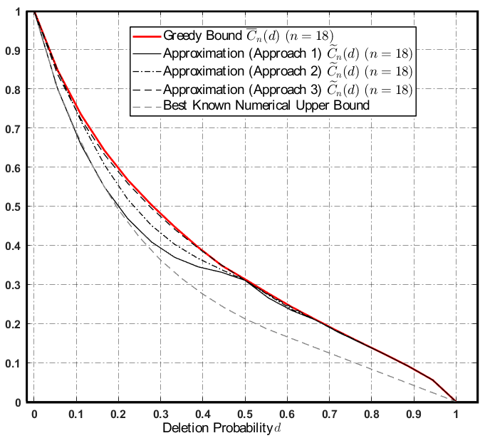
We compute the duplication ratios with different block-lengths nn and mm. We exemplify part of the results in Table I and Table II. Furthermore, setting n=18n=18, we plot the following quantities:

C¯n​(d):=\displaystyle\overline{C}_{n}(\mathit{d}):= 1n​log⁡(∑𝐲∈{0,1}⌈n⁡(1−d)⌉max𝐱∈{0,1}n⁡#⁡(𝐱,𝐲)),\displaystyle\frac{1}{n}\log\bigg(\sum_{\mathbf{y}\in\{0,1\}^{\lceil n(1-\mathit{d})\rceil}}\max_{\mathbf{x}\in\{0,1\}^{n}}\#\left({\mathbf{x}},{\mathbf{y}}\right)\bigg),
C~n​(d):=\displaystyle\widetilde{C}_{n}(\mathit{d}):= 1n​log⁡(∑𝐲∈{0,1}⌈n⁡(1−d)⌉max𝐱∈{0,1}n⁡#dup​(𝐱,𝐲)).\displaystyle\frac{1}{n}\log\bigg(\sum_{\mathbf{y}\in\{0,1\}^{\lceil n(1-\mathit{d})\rceil}}\max_{\mathbf{x}\in\{0,1\}^{n}}\#_{\mathrm{dup}}\left({\mathbf{x}},{\mathbf{y}}\right)\bigg).

The output block-length mm in above is set to be an integer between 11 and n=18n=18. In order to approximate the values of C¯n​(d)\overline{C}_{n}(\mathit{d}) and C~n​(d)\widetilde{C}_{n}(\mathit{d}) when mm is not divided by nn, we consider the following three different approaches:

Approach 1 (Assign-to-the-last Approximation):

First, duplicate ϝ\digamma times each bit in 𝐲\mathbf{y} where ϝ\digamma is the largest integer satisfying m​ϝ≤nm\digamma\leq n; then for the remaining n−m​ϝn-m\digamma bits, assign them proportionally to the last several runs in 𝐲\mathbf{y}. For instance, suppose m=6m=6, n=15n=15 and 𝐲=010001\mathbf{y}=010001. An approximation can be obtained by first constructing a length-1212 sequence by duplicating the bits in 𝐲\mathbf{y}; then assigning 11 bit to the last run and 22 bits to the second last run.

Approach 2 (Assign-by-the-length Approximation):

The first step is the same as Approach 1. For the remaining bits, longer runs get more bits, i.e., assign them to the longest run (of length ℓ\ell) until the length exceeds ℓ​n/⌊m⌋\ell n/\lfloor m\rfloor. For example, suppose m=6m=6, n=15n=15 and 𝐲=010001\mathbf{y}=010001. Then the formed new length-nn sequence is 001100000000011001100000000011.

Approach 3 (Gamma Function Approximation):

An alternative approximation is to substitute the binomial coefficients in Eq. (51) by Gamma functions, thus ensuring ϝ=n/m\digamma=n/m taking non-integers.

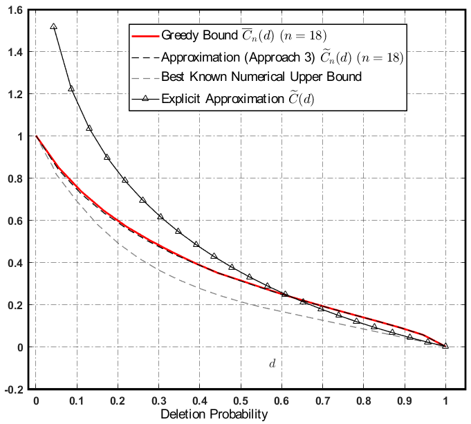
The three approximations of C~n​(d)\widetilde{C}_{n}(\mathit{d}) and the ML upper bound C¯n​(d)\overline{C}_{n}(\mathit{d}) are depicted in Figure 2, together with the best known numerical upper bounds reported in [22].

Refer to caption
Fig. 2: The ML upper bound (solid, red) C¯n​(d)\overline{C}_{n}(\mathit{d}) for BDC with block-length n=18n=18, together approximations of C~n​(d)\widetilde{C}_{n}(\mathit{d}) obtained via the three approaches. The lower curve (dashed gray) corresponds to the best known numerical upper bounds provided in [22].
 

Some observations are summarized as hypotheses in sequel.

(ℓ​ϝℓ)=(ℓ​ϝ)!ℓ!​(ℓ​ϝ−ℓ)!\displaystyle{\ell\digamma\choose\ell}=\frac{\left(\ell\digamma\right)!}{\ell!\left(\ell\digamma-\ell\right)!} ≤exp⁡(−ℓ​ϝ+1)​(ℓ​ϝ)ℓ​ϝ+1/2(2​π​exp⁡(−ℓ)​ℓℓ+1/2)⋅(2​π​exp⁡(−(ℓ​ϝ−ℓ))​(ℓ​ϝ−ℓ)(ℓ​ϝ−ℓ)+1/2)\displaystyle\leq\frac{\exp\left(-\ell\digamma+1\right)\left(\ell\digamma\right)^{\ell\digamma+1/2}}{\left(\sqrt{2\pi}\exp(-\ell)\ell^{\ell+1/2}\right)\cdot\left(\sqrt{2\pi}\exp(-\left(\ell\digamma-\ell\right))\left(\ell\digamma-\ell\right)^{\left(\ell\digamma-\ell\right)+1/2}\right)} (52)

 
Hypothesis 1.

For any block-lengths n,m∈ℕ+n,m\in\mathbbm{N}^{+} and ϝ=n/m∈ℕ+\digamma={n}/{m}\in\mathbbm{N}^{+},

min𝐲∈{0,1}n/ϝ⁡γ⁡(n,ϝ,𝐲)=ϝn/ϝ#¯​(𝐲flip)\displaystyle\min_{\mathbf{y}\in\{0,1\}^{{n}/{\digamma}}}\gamma\left(n,\digamma,\mathbf{y}\right)=\frac{\digamma^{{n}/{\digamma}}}{\overline{\#}\left({\mathbf{y}_{\mathrm{flip}}}\right)}

where 𝐲flip{\mathbf{y}_{\mathrm{flip}}} denotes a length-mm binary sequence with flipping bits, i.e., R𝐲(1)=mR^{(1)}_{\mathbf{y}}=m and R𝐲(ℓ)=0R^{(\ell)}_{\mathbf{y}}=0 for all ℓ>1\ell>1.

Moreover, the approximations are tight, such that

Hypothesis 2.

For any block-lengths n,m∈ℕ+n,m\in\mathbbm{N}^{+} and ϝ=n/m∈ℕ+\digamma={n}/{m}\in\mathbbm{N}^{+},

limn→∞1n​log⁡γ⁡(n,ϝ)=0.\displaystyle\lim_{n\rightarrow\infty}\frac{1}{n}\log\gamma\left(n,\digamma\right)=0.

Furthermore, based on Hypothesis 1, Hypothesis 2 is true when d→1\mathit{d}\rightarrow 1. Denote by γ⁡(n,ϝ):=min𝐲∈{0,1}n/ϝ⁡γ⁡(n,ϝ,𝐲)\gamma\left(n,\digamma\right):=\min_{\mathbf{y}\in\{0,1\}^{{n}/{\digamma}}}\gamma\left(n,\digamma,\mathbf{y}\right) for notational convenience. We conclude the following asymptotic behavior of γ⁡(n,ϝ,𝐲)\gamma\left(n,\digamma,\mathbf{y}\right):

Lemma 8.
limm/n→1limn→∞1n​log⁡γ⁡(n,ϝ)=0.\displaystyle\lim_{{m}/{n}\rightarrow 1}\lim_{n\rightarrow\infty}\frac{1}{n}\log\gamma\left(n,\digamma\right)=0.
Proof.

Noe that γ⁡(n,ϝ)=ϝn/ϝ#¯​(𝐲flip)≥ϝn/ϝ(nm)\gamma\left(n,\digamma\right)=\frac{\digamma^{{n}/{\digamma}}}{\overline{\#}\left({\mathbf{y}_{\mathrm{flip}}}\right)}\geq\frac{\digamma^{{n}/{\digamma}}}{{n\choose m}}. Using Stirling’s approximation (see (52)), we get

(nm)≤e2​π⋅2n​h​(mn)(1−mn)​m.\displaystyle{n\choose m}\leq\frac{e}{2\pi}\cdot\frac{2^{nh(\frac{m}{n})}}{\sqrt{\left(1-\frac{m}{n}\right)m}}.

Since ϝ=n/m\digamma=n/m,

γ⁡(n,ϝ)≥2​πe⋅(nm)m​(1−mn)​m2n​h​(mn).\displaystyle\gamma\left(n,\digamma\right)\geq\frac{2\pi}{e}\cdot\left(\frac{n}{m}\right)^{m}\frac{\sqrt{\left(1-\frac{m}{n}\right)m}}{2^{nh(\frac{m}{n})}}.

Thus, taking logarithm and letting n→∞n\rightarrow\infty,

limn→∞1n​log⁡γ⁡(n,ϝ)≥\displaystyle\lim_{n\rightarrow\infty}\frac{1}{n}\log\gamma\left(n,\digamma\right)\geq limn→∞1n​(m​log⁡nm−n​h​(mn))\displaystyle\lim_{n\rightarrow\infty}\frac{1}{n}\left(m\log\frac{n}{m}-nh\left(\frac{m}{n}\right)\right)
=\displaystyle= limn→∞(1−mn)​log⁡(11−m/n),\displaystyle\lim_{n\rightarrow\infty}\left(1-\frac{m}{n}\right)\log\left(\frac{1}{1-{m}/{n}}\right),

which goes to 00 as m/n→1{m}/{n}\rightarrow 1. ∎

The remaining part of this work is based on Hypothesis 2.

IV-D Explicit Approximation of C¯​(d)\overline{C}(\mathit{d})

Based on Hypothesis 2, we can further bound the capacity C⁡(d)C(\mathit{d}) of the BDC when the deletion probability d≥1/2\mathit{d}\geq 1/2.

Lemma 9.

Suppose Hypothesis 2 is true. For any block-lengths n,m∈ℕ+n,m\in\mathbbm{N}^{+} and ϝ=n/m∈ℕ+\digamma={n}/{m}\in\mathbbm{N}^{+}, the following bound on C⁡(d)C(\mathit{d}) holds:

C⁡(d)≤lim infn→∞1n​log​∑𝐲∈{0,1}m∏ℓ=1m(ℓ​ϝℓ)Rℓ​(𝐲)−h⁡(d)\displaystyle C(\mathit{d})\leq\liminf_{n\rightarrow\infty}\frac{1}{n}\log\sum_{\mathbf{y}\in\{0,1\}^{m}}{\prod_{\ell=1}^{m}{\ell\digamma\choose\ell}^{R_{\ell}\left({\mathbf{y}}\right)}}-h\left(\mathit{d}\right) (53)

where m=⌈n⁡(1−d)⌉m=\lceil n(1-\mathit{d})\rceil.

Proof.

We start with repeating Theorem 3:

C⁡(d)≤C¯​(d)=1n​log⁡(∑𝐲∈{0,1}m#¯​(𝐲))−h⁡(d)\displaystyle C(\mathit{d})\leq\overline{C}(\mathit{d})=\frac{1}{n}\log\Big(\sum_{\mathbf{y}\in\{0,1\}^{m}}\overline{\#}\left({\mathbf{y}}\right)\Big)-h\left(\mathit{d}\right) (54)

provided m=⌈n⁡(1−d)⌉m=\lceil n(1-\mathit{d})\rceil.

Suppose mm divides nn. Considering the definition of γ⁡(n,ϝ)\gamma\left(n,\digamma\right), the logarithmic term in above can be bounded as

1n​log​∑𝐲∈{0,1}m#¯​(𝐲)\displaystyle\frac{1}{n}\log\sum_{\mathbf{y}\in\{0,1\}^{m}}\overline{\#}\left({\mathbf{y}}\right)
≤\displaystyle\leq 1n​log⁡(∑𝐲∈{0,1}m∏ℓ=1m(ℓ​ϝℓ)R𝐲(ℓ)γ⁡(n,ϝ))\displaystyle\frac{1}{n}\log\Bigg(\sum_{\mathbf{y}\in\{0,1\}^{m}}\frac{\prod_{\ell=1}^{m}{\ell\digamma\choose\ell}^{R^{(\ell)}_{\mathbf{y}}}}{\gamma\left(n,\digamma\right)}\Bigg)
=\displaystyle= 1n​log⁡(∑𝐲∈{0,1}m∏ℓ=1m(ℓ​ϝℓ)R𝐲(ℓ))−1n​log⁡γ⁡(n,ϝ)\displaystyle\frac{1}{n}\log\Bigg(\sum_{\mathbf{y}\in\{0,1\}^{m}}{\prod_{\ell=1}^{m}{\ell\digamma\choose\ell}^{R^{(\ell)}_{\mathbf{y}}}}\Bigg)-\frac{1}{n}\log\gamma\left(n,\digamma\right) (55)

Taking the limits n→∞n\rightarrow\infty and d→1\mathit{d}\rightarrow 1, Hypothesis 2 implies (53). ∎

We will then show the following lemma holds:

Lemma 10.

Suppose m=⌈n⁡(1−d)⌉m=\lceil n(1-\mathit{d})\rceil. For all deletion probability d∈[1/2,1)\mathit{d}\in[1/2,1),

1n​log​∑𝐲∈{0,1}m∏ℓ=1m(ℓ​ϝℓ)Rℓ​(𝐲)\displaystyle\frac{1}{n}\log\sum_{\mathbf{y}\in\{0,1\}^{m}}{\prod_{\ell=1}^{m}{\ell\digamma\choose\ell}^{R_{\ell}\left({\mathbf{y}}\right)}}
=\displaystyle= h⁡(d)+1−d+1n​log⁡(𝔼⁡[exp⁡(−μd​(𝐘))])\displaystyle h(\mathit{d})+1-\mathit{d}+\frac{1}{n}\log\Big(\mathbbm{E}\big[\exp\left({-\mu_{\mathit{d}}\left({\mathbf{Y}}\right)}\right)\big]\Big) (56)

where

μd​(𝐲):=\displaystyle\mu_{\mathit{d}}\left({\mathbf{y}}\right):= 12​∑ℓ=1mR𝐲(ℓ)​ln⁡((2​πe)2​d​ℓ),\displaystyle\frac{1}{2}\sum_{\ell=1}^{m}R^{(\ell)}_{\mathbf{y}}\ln\left(\left(\frac{2\pi}{e}\right)^{2}\mathit{d}\ell\right),

and the expectation is over a random length-mm sequence 𝐘\mathbf{Y} wherein each bit is a random variable with distribution Bernoulli⁡(1/2)\mathrm{Bernoulli}\left({1}/{2}\right).

Proof.

Applying Stirling’s approximation (inequalities) to the binomial coefficients, (53) follows. Therefore

(ℓ​ϝℓ)\displaystyle{\ell\digamma\choose\ell} ≤e​(ℓ​ϝ)ℓ​ϝ+1/22​π​ℓℓ+1/2​(ℓ​ϝ−ℓ)(ℓ​ϝ−ℓ)+1/2\displaystyle\leq\frac{e\left(\ell\digamma\right)^{\ell\digamma+1/2}}{2\pi\ell^{\ell+1/2}\left(\ell\digamma-\ell\right)^{\left(\ell\digamma-\ell\right)+1/2}}
=e2​π⋅(ℓ​ϝ)ℓ​ϝℓℓ​(ℓ​ϝ−ℓ)(ℓ​ϝ−ℓ)⋅ϝℓ⁡(ϝ−1).\displaystyle=\frac{e}{2\pi}\cdot\frac{\left(\ell\digamma\right)^{\ell\digamma}}{\ell^{\ell}\left(\ell\digamma-\ell\right)^{\left(\ell\digamma-\ell\right)}}\cdot\sqrt{\frac{\digamma}{\ell\left(\digamma-1\right)}}. (57)

Since ϝ=11−d\digamma=\frac{1}{1-\mathit{d}}, we have ϝϝ−1=1d\frac{\digamma}{\digamma-1}=\frac{1}{\mathit{d}}. Thus,

(ℓ​ϝ)ℓ​ϝℓℓ​(ℓ​ϝ−ℓ)(ℓ​ϝ−ℓ)\displaystyle\frac{\left(\ell\digamma\right)^{\ell\digamma}}{\ell^{\ell}\left(\ell\digamma-\ell\right)^{\left(\ell\digamma-\ell\right)}} =2ℓ​ϝ​h​((ϝ−1)/ϝ)=2ℓ​ϝ​h​(d),\displaystyle=2^{\ell\digamma h\left({\left(\digamma-1\right)}/{\digamma}\right)}=2^{\ell\digamma h(\mathit{d})}, (58)
ϝℓ⁡(ϝ−1)\displaystyle\sqrt{\frac{\digamma}{\ell\left(\digamma-1\right)}} =1d​ℓ.\displaystyle=\sqrt{\frac{1}{\mathit{d}\ell}}. (59)

Putting (58) and (59) into (57),

(ℓ​ϝℓ)≤e2​π⋅2ℓ​ϝ​h​(d)d​ℓ.\displaystyle{\ell\digamma\choose\ell}\leq\frac{e}{2\pi}\cdot\frac{2^{\ell\digamma h(\mathit{d})}}{\sqrt{\mathit{d}\ell}}.

Therefore,

ln⁡(∏ℓ=1m(ℓ​ϝℓ)R𝐲(ℓ))\displaystyle\ln\left(\prod_{\ell=1}^{m}{\ell\digamma\choose\ell}^{R^{(\ell)}_{\mathbf{y}}}\right)
=\displaystyle= ∑ℓ=1mR𝐲(ℓ)​ln⁡(ℓ​ϝℓ)\displaystyle\sum_{\ell=1}^{m}R^{(\ell)}_{\mathbf{y}}\ln{\ell\digamma\choose\ell}
≤\displaystyle\leq ∑ℓ=1m(ln⁡2)​ℓ​R𝐲(ℓ)​ϝ​h​(d)\displaystyle\sum_{\ell=1}^{m}\left({\ln 2}\right)\ell R^{(\ell)}_{\mathbf{y}}\digamma h(\mathit{d})
+∑ℓ=1mR𝐲(ℓ)lne2​π−12∑ℓ=1mR𝐲(ℓ)ln(dℓ).\displaystyle+\sum_{\ell=1}^{m}R^{(\ell)}_{\mathbf{y}}\ln\frac{e}{2\pi}-\frac{1}{2}\sum_{\ell=1}^{m}R^{(\ell)}_{\mathbf{y}}\ln\left(\mathit{d}\ell\right).

According to (49), ∑ℓ=1mℓ​R𝐲(ℓ)=m\sum_{\ell=1}^{m}\ell R^{(\ell)}_{\mathbf{y}}=m, implying that

∑ℓ=1mℓ​R𝐲(ℓ)​ϝ​h​(d)=m​ϝ​h​(d)=n​h​(d).\displaystyle\sum_{\ell=1}^{m}\ell R^{(\ell)}_{\mathbf{y}}\digamma h(\mathit{d})=m\digamma h(\mathit{d})=nh(\mathit{d}).

Continuing from above,

ln⁡(∏ℓ=1m(ℓ​ϝℓ)R𝐲(ℓ))\displaystyle\ln\left(\prod_{\ell=1}^{m}{\ell\digamma\choose\ell}^{R^{(\ell)}_{\mathbf{y}}}\right)
≤\displaystyle\leq (ln⁡2)​n​h​(d)+∑ℓ=1mR𝐲(ℓ)​ln⁡e2​π−12​∑ℓ=1mR𝐲(ℓ)​ln⁡(d​ℓ)\displaystyle\left({\ln 2}\right)nh(\mathit{d})+\sum_{\ell=1}^{m}R^{(\ell)}_{\mathbf{y}}\ln\frac{e}{2\pi}-\frac{1}{2}\sum_{\ell=1}^{m}R^{(\ell)}_{\mathbf{y}}\ln\left(\mathit{d}\ell\right) (60)
=\displaystyle= (ln⁡2)​n​h​(d)−12​∑ℓ=1mR𝐲(ℓ)​ln⁡((2​πe)2​d​ℓ).\displaystyle\left({\ln 2}\right)nh(\mathit{d})-\frac{1}{2}\sum_{\ell=1}^{m}R^{(\ell)}_{\mathbf{y}}\ln\left(\left(\frac{2\pi}{e}\right)^{2}\mathit{d}\ell\right). (61)

Recall that

μd​(𝐲):=12​∑ℓ=1mR𝐲(ℓ)​ln⁡((2​πe)2​d​ℓ).\displaystyle\mu_{\mathit{d}}\left({\mathbf{y}}\right):=\frac{1}{2}\sum_{\ell=1}^{m}R^{(\ell)}_{\mathbf{y}}\ln\left(\left(\frac{2\pi}{e}\right)^{2}\mathit{d}\ell\right).

Thus, summing over all 𝐲∈{0,1}m\mathbf{y}\in\{0,1\}^{m}, (61) yields that

1n​log​∑𝐲∈{0,1}m∏ℓ=1m(ℓ​ϝℓ)Rℓ​(𝐲)\displaystyle\frac{1}{n}\log\sum_{\mathbf{y}\in\{0,1\}^{m}}{\prod_{\ell=1}^{m}{\ell\digamma\choose\ell}^{R_{\ell}\left({\mathbf{y}}\right)}}
≤\displaystyle\leq 1n​log​∑𝐲∈{0,1}mexp⁡((ln⁡2)​n​h​(d)−μd​(𝐲))\displaystyle\frac{1}{n}\log\sum_{\mathbf{y}\in\{0,1\}^{m}}\exp\big(\left({\ln 2}\right){nh(\mathit{d})-\mu_{\mathit{d}}\left({\mathbf{y}}\right)}\big) (62)
=\displaystyle= h⁡(d)+1n​log​∑𝐲∈{0,1}mexp⁡(−μd​(𝐲)).\displaystyle h(\mathit{d})+\frac{1}{n}\log\sum_{\mathbf{y}\in\{0,1\}^{m}}\exp\big({-\mu_{\mathit{d}}\left({\mathbf{y}}\right)}\big).

The summation ∑𝐲∈{0,1}mexp⁡(−μd​(𝐲))\sum_{\mathbf{y}\in\{0,1\}^{m}}\exp\left({-\mu_{\mathit{d}}\left({\mathbf{y}}\right)}\right) can be regarded as 2m2^{m} times the expectation of exp⁡(−μd​(𝐘))\exp\left({-\mu_{\mathit{d}}\left({\mathbf{Y}}\right)}\right) given that each bit in 𝐘\mathbf{Y} is selected Bernoulli⁡(1/2)\mathrm{Bernoulli}\left({1}/{2}\right). Therefore,

1n​log​∑𝐲∈{0,1}m∏ℓ=1m(ℓ​ϝℓ)Rℓ​(𝐲)\displaystyle\frac{1}{n}\log\sum_{\mathbf{y}\in\{0,1\}^{m}}{\prod_{\ell=1}^{m}{\ell\digamma\choose\ell}^{R_{\ell}\left({\mathbf{y}}\right)}}
≤\displaystyle\leq h⁡(d)+1n​log⁡(2m​𝔼​[exp⁡(−μd​(𝐘))])\displaystyle h(\mathit{d})+\frac{1}{n}\log\Big(2^{m}\mathbbm{E}\big[\exp\left({-\mu_{\mathit{d}}\left({\mathbf{Y}}\right)}\right)\big]\Big)
=\displaystyle= h⁡(d)+1−d+1n​log⁡(𝔼⁡[exp⁡(−μd​(𝐘))]).\displaystyle h(\mathit{d})+1-\mathit{d}+\frac{1}{n}\log\Big(\mathbbm{E}\big[\exp\left({-\mu_{\mathit{d}}\left({\mathbf{Y}}\right)}\right)\big]\Big). (63)

∎

Taking the expectation outside, we derive the following approximation of the last term in (63):

1n​𝔼​[log⁡(exp⁡(−μd​(𝐘)))]=−1n​𝔼​[(log⁡e)​μd​(𝐘)].\displaystyle\frac{1}{n}\mathbbm{E}\Big[\log\big(\exp\left({-\mu_{\mathit{d}}\left({\mathbf{Y}}\right)}\right)\big)\Big]=-\frac{1}{n}\mathbbm{E}\big[{\left(\log e\right)\mu_{\mathit{d}}\left({\mathbf{Y}}\right)}\big]. (64)

For a Bernoulli⁡(1/2)\mathrm{Bernoulli}\left({1}/{2}\right) process, the distribution of the number of ℓ\ell-runs R𝐲(1)R^{(1)}_{\mathbf{y}},…,R𝐲(m)\ldots,R^{(m)}_{\mathbf{y}} is proportional to the “run-length distribution” defined in [25], which is {1/2ℓ}ℓ=1∞\{1/2^{\ell}\}_{\ell=1}^{\infty}. Hence, considering (49), the expectation of the number of runs is m/2ℓ+1{m}/{2^{\ell+1}}, i.e.,

𝔼⁡[R𝐘(ℓ)]=m2ℓ+1.\displaystyle\mathbbm{E}\big[R^{(\ell)}_{\mathbf{Y}}\big]=\frac{m}{2^{\ell+1}}.

It follows that

𝔼​[μd​(𝐘)]=\displaystyle\mathbbm{E}\big[{\mu_{\mathit{d}}\left({\mathbf{Y}}\right)}\big]= 𝔼⁡[12​∑ℓ=1mR𝐲(ℓ)​ln⁡((2​πe)2​d​ℓ)]\displaystyle\mathbbm{E}\Bigg[\frac{1}{2}\sum_{\ell=1}^{m}R^{(\ell)}_{\mathbf{y}}\ln\left(\left(\frac{2\pi}{e}\right)^{2}\mathit{d}\ell\right)\Bigg]
=\displaystyle= 12​∑ℓ=1m𝔼⁡[R𝐘(ℓ)]​ln⁡((2​πe)2​d​ℓ)\displaystyle\frac{1}{2}\sum_{\ell=1}^{m}\mathbbm{E}\big[R^{(\ell)}_{\mathbf{Y}}\big]\ln\left(\left(\frac{2\pi}{e}\right)^{2}\mathit{d}\ell\right)
=\displaystyle= m2​∑ℓ=1m12ℓ+1​ln⁡((2​πe)2​d​ℓ).\displaystyle\frac{m}{2}\sum_{\ell=1}^{m}\frac{1}{2^{\ell+1}}\ln\left(\left(\frac{2\pi}{e}\right)^{2}\mathit{d}\ell\right). (65)

Combining (53), (56), the approximation (65) and the identity (64) above, the approximation C~​(d)\widetilde{C}(\mathit{d}) defined below holds:

C~​(d):=\displaystyle\widetilde{C}(\mathit{d}):= 1−d−limn→∞1n​𝔼​[(log⁡e)​μd​(𝐘)]\displaystyle 1-\mathit{d}-\lim_{n\rightarrow\infty}\frac{1}{n}\mathbbm{E}\big[{\left(\log e\right)\mu_{\mathit{d}}\left({\mathbf{Y}}\right)}\big]
=\displaystyle= 1−d−12​ψ​(1−d)\displaystyle 1-\mathit{d}-\frac{1}{2}\psi\left(1-\mathit{d}\right) (66)

where

ψ:=\displaystyle\psi:= ∑ℓ=1∞12ℓ+1​log⁡((2​πe)2​d​ℓ)\displaystyle\sum_{\ell=1}^{\infty}\frac{1}{2^{\ell+1}}\log\left(\left(\frac{2\pi}{e}\right)^{2}\mathit{d}\ell\right)
=\displaystyle= 12​log⁡d+∑ℓ=1∞log⁡((2​π/e)​ℓ)2ℓ≲12​log⁡d+1.09179.\displaystyle\frac{1}{2}\log\mathit{d}+\sum_{\ell=1}^{\infty}\frac{\log\left(\left({2\pi}/{e}\right)\sqrt{\ell}\right)}{2^{\ell}}\lesssim\frac{1}{2}\log\mathit{d}+1.09179.

A figure depicting the explicit approximation C~​(d)\widetilde{C}(\mathit{d}) for d≥1/2\mathit{d}\geq 1/2 is provided below.

Refer to caption
Fig. 3: The ML upper bound (solid, red) C¯n​(d)\overline{C}_{n}(\mathit{d}) for BDC with block-length n=18n=18, the approximation of C~n​(d)\widetilde{C}_{n}(\mathit{d}) obtained via the gamma function, and the explicit approximation C~​(d)\widetilde{C}(\mathit{d}) derived in (66). The lower curve (dashed gray) corresponds to the best known numerical upper bounds provided in [22].
 

V Conclusion

We derive a general ML upper bound (See Theorem 1) for information stable channels. The corresponding bounds are shown to be tight for simple channels, e.g., the BEC and the BSC. Furthermore, we demonstrate the usage of the bound on the BDC, whose capacity remains unknown. The corresponding upper bound for the BDC derived from the general bound coincides with an intriguing combinatorial problem (defined as the MDM problem in Definition 10). Approximations for the derived upper bound are provided via three different approaches. Furthermore, analyzing and approximating the limiting behavior of the derived upper bound gives an explicit bound reported in (66) (and shown in Figure 3), validating that the general bound is capable of providing nontrivial results for sophisticated channels with memory. The next step is to validate the upper bounds on a varriety types of channels and formalize a more general framework based on the main result (Theorem 1) stated in the paper.

References

  • [1] R. Dobrushin, “General formulation of shannon’s main theorem in information theory,” Amer. Math. Soc. Trans, vol. 33, pp. 323–438, 1963.
  • [2] G. Hu, “On shannon theorem and its converse for sequence of communication schemes in the case of abstract random variables,” in Trans. 3rd Prague Conference on Information Theory, Statistical Decision Functions, Random Processes, Czechslovak Academy of Sciences, Prague, 1964, pp. 285–333.
  • [3] S. Verdu and T. Han, “A general formula for channel capacity,” Information Theory, IEEE Transactions on, vol. 40, no. 4, pp. 1147–1157, 1994.
  • [4] S. Tatikonda and S. Mitter, “The capacity of channels with feedback,” IEEE Transactions on Information Theory, vol. 55, no. 1, pp. 323–349, 2009.
  • [5] M. Hayashi and H. Nagaoka, “General formulas for capacity of classical-quantum channels,” IEEE Transactions on Information Theory, vol. 49, no. 7, pp. 1753–1768, 2003.
  • [6] V. I. Levenshtein, “Binary codes capable of correcting deletions, insertions and reversals,” in Soviet physics doklady, vol. 10, 1966, p. 707.
  • [7] R. L. Dobrushin, “Shannon’s theorems for channels with synchronization errors,” Problemy Peredachi Informatsii, vol. 3, no. 4, pp. 18–36, 1967.
  • [8] S. Arimoto, “An algorithm for computing the capacity of arbitrary discrete memoryless channels,” Information Theory, IEEE Transactions on, vol. 18, no. 1, pp. 14–20, 1972.
  • [9] R. E. Blahut, “Computation of channel capacity and rate-distortion functions,” Information Theory, IEEE Transactions on, vol. 18, no. 4, pp. 460–473, 1972.
  • [10] D. Fertonani and T. M. Duman, “Novel bounds on the capacity of the binary deletion channel,” Information Theory, IEEE Transactions on, vol. 56, no. 6, pp. 2753–2765, 2010.
  • [11] S. Vembu, S. Verdù, and Y. Steinberg, “The source-channel separation theorem revisited,” Information Theory, IEEE Transactions on, vol. 41, no. 1, pp. 44–54, 1995.
  • [12] T. Han and S. Verdu, “Approximation theory of output statistics,” Information Theory, IEEE Transactions on, vol. 39, no. 3, pp. 752–772, 1993.
  • [13] P.-N. Chen and F. Alajaji, “Optimistic shannon coding theorems for arbitrary single-user systems,” Information Theory, IEEE Transactions on, vol. 45, no. 7, pp. 2623–2629, 1999.
  • [14] A. Feinstein, A new basic theorem of information theory, 1954.
  • [15] C. E. Shannon, “Certain results in coding theory for noisy channels,” Information and control, vol. 1, no. 1, pp. 6–25, 1957.
  • [16] R. G. Gallager, Information theory and reliable communication. Springer, 1968, vol. 2.
  • [17] F. Jelinek, Probabilistic information theory: discrete and memoryless models. McGraw-Hill, 1968.
  • [18] M. Mitzenmacher et al., “A survey of results for deletion channels and related synchronization channels,” Probability Surveys, vol. 6, pp. 1–33, 2009.
  • [19] H. Chernoff, “A note on an inequality involving the normal distribution,” The Annals of Probability, pp. 533–535, 1981.
  • [20] M. Mitzenmacher and E. Upfal, Probability and computing: Randomized algorithms and probabilistic analysis. Cambridge University Press, 2005.
  • [21] M. Cheraghchi, “Capacity upper bounds for deletion-type channels,” arXiv preprint arXiv:1711.01630, 2017.
  • [22] M. Rahmati and T. M. Duman, “Upper bounds on the capacity of deletion channels using channel fragmentation,” Information Theory, IEEE Transactions on, vol. 61, no. 1, pp. 146–156, 2015.
  • [23] S. Diggavi, M. Mitzenmacher, and H. Pfister, “Capacity upper bounds for deletion channels,” in Proceedings of the International Symposium on Information Theory, 2007, pp. 1716–1720.
  • [24] M. Dalai, “A new bound on the capacity of the binary deletion channel with high deletion probabilities,” in Information Theory Proceedings (ISIT), 2011 IEEE International Symposium on. IEEE, 2011, pp. 499–502.
  • [25] Y. Kanoria and A. Montanari, “Optimal coding for the binary deletion channel with small deletion probability,” Information Theory, IEEE Transactions on, vol. 59, no. 10, pp. 6192–6219, 2013.
  • [26] A. Kalai, M. Mitzenmacher, and M. Sudan, “Tight asymptotic bounds for the deletion channel with small deletion probabilities,” in Information Theory Proceedings (ISIT), 2010 IEEE International Symposium on. IEEE, 2010, pp. 997–1001.
  • [27] M. Drmota, W. Szpankowski, and K. Viswanathan, “Mutual information for a deletion channel,” in Information Theory Proceedings (ISIT), 2012 IEEE International Symposium on. IEEE, 2012, pp. 2561–2565.
  • [28] H. Koga et al., Information-spectrum methods in information theory. Springer Science & Business Media, 2013, vol. 50.
  • [29] Y. Liron and M. Langberg, “A characterization of the number of subsequences obtained via the deletion channel,” IEEE Transactions on Information Theory, vol. 61, no. 5, pp. 2300–2312, 2015.
  • [30] J. Bourdon and B. Vallée, “Generalized pattern matching statistics,” in Mathematics and Computer Science II. Springer, 2002, pp. 249–265.
  • [31] A. Kirsch and E. Drinea, “Directly lower bounding the information capacity for channels with iid deletions and duplications,” Information Theory, IEEE Transactions on, vol. 56, no. 1, pp. 86–102, 2010.