Multi-Rate Time Integration on Overset Meshes
Abstract
Overset meshes are an effective tool for the computational fluid dynamic simulation of problems with complex geometries or multiscale spatio-temporal features. When the maximum allowable timestep on one or more meshes is significantly smaller than on the remaining meshes, standard explicit time integrators impose inefficiencies for time-accurate calculations by requiring that all meshes advance with the smallest timestep. With the targeted use of multi-rate time integrators, separate meshes can be time-marched at independent rates to avoid wasteful computation while maintaining accuracy and stability. This work applies time-explicit multi-rate integrators to the simulation of the compressible Navier-Stokes equations discretized on overset meshes using summation-by-parts (SBP) operators and simultaneous approximation term (SAT) boundary conditions. We introduce a class of multi-rate Adams-Bashforth (MRAB) schemes that offer significant stability improvements and computational efficiencies for SBP-SAT methods. We present numerical results that confirm the efficacy of MRAB integrators, outline a number of implementation challenges, and demonstrate a reduction in computational cost enabled by MRAB. We also investigate the use of our method in the setting of a large-scale distributed-memory parallel implementation where we discuss concerns involving load balancing and communication efficiency.
Keywords:
Multi-Rate Time Integration, Overset Meshes, Chimera, Summation-By-Parts, Simultaneous-Approximation-Term, Adams-Bashforth.1 Introduction
In the time-explicit direct numerical simulation (DNS) of computational fluid dynamic problems, the maximum timestep allowable for stable integration of the governing equations is often limited by the well-known Courant-Friedrichs-Lewy number (CFL),
where is the minimum grid spacing, and is the maximum characteristic speed of the physical phenomena being simulated, or its viscous analog,
where is the characteristic diffusivity. The timestep taken when integrating over the entire computational domain using a standard explicit single-rate integrator can be limited by dynamics that occur on a small portion of the domain, be it due to shorter time scales of certain physical phenomena, such as high-speed flow, or locally-high grid resolution.
With multi-rate integration, groups of degrees of freedom, or even individual right-hand side contributions corresponding to evolution on small timescales, can be integrated with independent time steps, allowing computational work to be avoided on the “slow” components while the “fast” components remain stable and well-resolved in time. This has the potential to improve the efficiency of the application. The present study focuses on an application of multi-rate integrators to problems with overset meshes.
The method of overset meshes (also known as the Chimera method [56]) is an approach that discretizes a domain using multiple independent, overlapping structured meshes, each of which is associated with a smooth but potentially geometrically complex mapping. The earliest known appearance of a composite mesh method was to solve elliptic partial differential equations [65], but similar methods were soon introduced for inviscid transonic flow [37] and the Euler equations of gas dynamics [5]. Some of the earliest analysis of stability was performed by Starius, who examined the stability of composite mesh methods for both elliptic boundary value problems [54] and hyperbolic systems of equations [55]. In the years since, high-order overset-grid (HO-OG) approaches have been developed [52, 12, 13] and applied to numerous problems [34, 50, 14, 25, 26, 53]. The individual meshes are structured, so that the entire discretization can be considered locally structured and globally unstructured. A concise summary of recent developments in the usage of overset meshes to solve problems involving compressible viscous fluids, along with a discussion of stable and accurate interpolation, is given in [10]. Additionally, a discussion of various applications of overset meshes can be found in [39].
Adaptive mesh refinement methods are similar to overset grid methods in that they address the need for locally high spatial resolution while also inherently introducing timescale disparity [7]. In particular, Berger et. al applied an automatic adaptive mesh refinement method to a hydrodynamic shock problem in two dimensions [6], along with hyperbolic conservation laws in three dimensions [4].
Some of the earliest work on multi-rate multistep methods was done by Gear [18]. Gear and Wells [19] later worked with these methods to automate the choice of step size and the partition of fast and slow components. The primary conclusion therein was that the problem of automating these integrator characteristics dynamically was mostly a function of software organization. Engstler and Lubich [17] used Richardson extrapolation along with simple Euler schemes to create a dynamically partitioned process of multi-rate integration.
Local timestepping methods are related to multi-rate time integration. Osher and Sanders [40] introduced numerical approximations to conservation laws that changed the global CFL restrictions to local ones. Dawson and Kirby [16] performed local time stepping based on the work of Osher and Sanders, attaining only first-order accuracy in time. Tang and Warnecke [64] expanded on this work to produce second-order accuracy via more refined projections of solution increments at each local timestep.
Günther, Kværnø, and Rentrop [21] introduced multi-rate partitioned Runge-Kutta (MPRK) schemes, starting from a discussion of Rosenbrock-Wanner methods, and based on strategies introduced by Günther and Rentrop [20]. These methods focus on coupling the fast and slow solution components primarily via interpolation and extrapolation of state variables, echoing the earlier work in [18] and [19].
Savcenco et. al [45] developed a self-adjusting multi-rate timestepping strategy primarily using implicit Rosenbrock methods on stiff ODEs. Constantinescu and Sandu [15] developed multi-rate timestepping methods for hyperbolic conservation laws based on a method of lines (MOL) approach with partitioned Runge-Kutta schemes. More recently, Sandu and Constantinescu [43] developed explicit multi-rate Adams-Bashforth methods similar to the ones discussed in this work, and while the resulting methods are exactly conservative, the computational experiments shown are limited to one-dimensional hyperbolic conservation laws, and the temporal accuracy of the methods is limited to second order by an interface region.
Recently, Seny and Lambrechts extended the explicit multi-rate Runge-Kutta schemes of Constantinescu and Sandu [15, 43] to apply to discontinuous Galerkin computations for large-scale geophysical flows, introducing the method [46] and subsequently demonstrating its efficacy in both serial and parallel implementations. Their latest work [47] focuses on efficient parallelization of the method using a multi-constraint partitioning library.
While all of these works characterize the stability of the multi-rate integrators numerically, only a few of them approach the topic of stability theoretically. An analytical discussion of the stability of a multi-rate method (namely, for numerical integration of a system of first-order ODEs that can be readily separated into subsystems) is given by Andrus in [1] whose study combines a fourth-order Runge-Kutta scheme (for the fast component) with a similar third-order scheme (for the slow component), introduced by the same author in [2]. Kværnøalso derived analytical expressions to find stability regions for her multi-rate Runge-Kutta schemes in [33].
In the present study, we use a multi-rate Adams-Bashforth integrator with enhanced stability in a distributed-memory parallel fluid solver, taking advantage of the solver’s overset mesh capabilities to segregate solution components with differing timescales. We do so with particular focus on the resulting improvement in performance, reduction in work through fewer right-hand-side evaluations, and accompanying changes in stability and accuracy. What results from this effort is a number of conclusions about the viability and extensibility of these integrators to other problems and applications. We couple our multi-rate Adams-Bashforth integrators with a summation-by-parts–simultaneous-approximation-term (SBP-SAT) method [58, 11, 38, 63, 61, 9], in particular with the newly-developed SBP-SAT-based interpolation method [49], to produce an accurate, efficient, and high-order approach to solving PDE-based problems. Our approach generalizes prior work on non-overset-based multi-rate methods [16, 64, 40, 15, 43] and removes constraints on temporal order of accuracy. We also introduce extended-history Adams-Bashforth schemes as a basis for a new class of multi-rate integrators that demonstrate improved stability compared to standard multi-rate Adams-Bashforth (MRAB) schemes. For further reference on some of the multi-rate Adams-Bashforth schemes implemented here, thorough analyses (especially empirical analyses of stability and the effect of various method design choices) are given in Klöckner [29]. Some related methods are also discussed in a particle-in-cell context by Stock [57].
2 Background
2.1 The Compressible Navier-Stokes Equations on Overset Meshes
We apply multi-rate integrators to the compressible Navier-Stokes equations on overset meshes, making use of an SBP-SAT discretization with a SAT-based method that applies the effect of an interpolation as a penalty term in the right-hand side. Details on the Navier-Stokes formulation, including the governing equations, nondimensionalization, and coordinate mappings can be found in [48]. Details on SBP operators can be found in [58, 11, 38]. For the results given later, we use the third-order SBP operator given in [38]. Details on the accompanying SAT boundary conditions can be found in [63, 61, 9]. For single-grid realizations of the scheme, the SBP-SAT discretizations we use have been shown [63, 61] to be provably stable for the compressible Navier-Stokes equations in three dimensions. For overset-grid realizations in two or three dimensions, no energy stability proof has yet been found.
2.2 SAT-Based Interpolation
The method used for interpolation between overset meshes is critical to the use of multi-rate integrators, as it forms the coupling between the fast and slow components. For consistency, it is important that communication between grids occurs through right-hand side increments rather than by direct interpolation and injection of state, given that the multi-rate schemes we will develop later are based upon multi-step schemes that depend directly upon accurate right-hand side histories and strictly ODE-based time advancement of the state.
Our interpolation relies on a Chimera framework inspired by the approach taken by the PEGASUS [59] and BELLERO [51] tools. In general, the process of communication between grids can be broken down into a number of phases:
- •
Establishing communication between grids. Compute the bounding box for a given grid, and use it to determine collisions with any other grids.
- •
Hole cutting/fringe determination. Identify points on each grid as "fringe points" which will donate and receive data from other grids, and identify points on coarser background grids which are well within the boundaries of the finer feature grids, and can thus be deemed inactive.
- •
Donor-receiver pair search — see Figure 1. Fringe points on the receiver grid are paired with donor cells on the donor grid.
- •
Interpolation. State data from the points in the donor cell is transferred to the receiver point via Lagrangian interpolation, with corresponding weights determined as a function of Lagrange shape functions.

See [10] for further discussion of this implementation, including algorithms for hole-cutting and the donor-receiver pair search. Once the donor data is sent (interpolated) to the receiver grids, it must be applied to the receiver state. The conventional method of interpolation between overset meshes uses an “injection” procedure to apply the result of overset interpolation, in which the state values on the receiver grid are directly overwritten by the interpolated values from the donor grid. The interpolation itself is performed at each right-hand side evaluation. This “injection" procedure is demonstrated in [49] to be unstable for the Euler equations in two dimensions. Injection-based interpolation schemes have been also used with SBP operators by Sjögreen et. al [53] and with adaptive mesh refinement codes [7, 6, 4] and have obtained conservation via interpolation of fluxes rather than state.
An alternative interface treatment given in [49] follows a methodology similar to the weak boundary treatment using SAT [63, 61, 9] and applies the interpolated values as a penalization term in the right-hand side via a target vector. Using the same notation as [49], we describe the overlapping interface as a boundary where , , or . is the normal direction to the face on which the grid point lies, and the superscript indicates inflow () or outflow (). If denotes the solution at a grid point on the interface, with the interpolated value from the donor grid given as , we can express the discretized equation at this point as
| (2.1) |
where denotes the derivatives of the fluxes, , is the (1,1) element of the positive-definite matrix associated with the SBP operator, is an identity matrix of size , and , where and are the transformation and diagonal matrices defined in [63, 61, 9]. denotes the viscous flux at the interface point, and all "hatted" terms indicate interpolated values. Note also that if the grid point lies on an edge or a corner in 3 dimensions, the interface terms for each of the three directions normal to the edge, or all directions in the case of a corner, must be added. The penalty parameters used in (2.1) are chosen as
for an inflow () or outflow () interface point. This scheme is shown in [49] to be provably time-stable for one-dimensional hyperbolic systems using SBP-SAT discretizations of up to global fourth-order accuracy on overlapping grids. In addition, a number of numerical examples, including extension of the scheme to both the two-dimensional Euler equations and the three-dimensional compressible Navier-Stokes equations for both Cartesian and curvilinear grids, demonstrate both stability and superior numerical characteristics compared to the injection method while also removing the need for artificial damping or filtering. Furthermore, proper convergence to the design order of accuracy is demonstrated with the use of this scheme in conjunction with SBP 1-2-1, SBP 2-4-2, and SBP 3-6-3 schemes on the Euler equations in multiple dimensions.
The injection-based method described in [10] is incompatible with the strictly ODE-based time advancement required for the schemes we will describe. Multi-step schemes are explicitly reliant on maintaining accurate right-hand side histories, whereas injection methods rely on in-place modification of state variables. The SAT interface treatment of [49] instead applies the effects of inter-grid communication as a right-hand side penalty, and is the method we will use.
The expected order of convergence for overset cases using this interpolation scheme in conjunction with a 3rd-order SBP-SAT spatial discretization is demonstrated using the method of manufactured solutions for the right-hand-side of the compressible Navier-Stokes equations (Eq. 2.1) as well as on analytical solutions for the inviscid (convecting vortex) and viscous (shock wave) forms of the equations. These results are given in C.
3 Time Integration
3.1 Adams-Bashforth Integration
To fix notation for new schemes developed later, we give a brief derivation of a standard Adams-Bashforth (AB) integrator, as described in [3]. We start with a model IVP given by
This is the form that results from a method of lines (MOL) approach to solving time-dependent partial differential equations like those considered in this study. We approximate the time dependency of the right-hand side function with a polynomial with coefficients (formed by interpolating past values of ), extrapolate with that polynomial approximation, and integrate the extrapolant. We use a Vandermonde matrix to construct a linear system to obtain the coefficients to be used in extrapolation from history values:
| (3.1) |
where is a vector evaluating the integral of the interpolation polynomial, and is the Vandermonde matrix with monomial basis and nodes , corresponding to past time values. In (3.1), is equal to the order of the integrator, and are the time history values, with . The coefficients are used to extrapolate to the next state via
| (3.2) |
Clearly, the length of the past history needed to calculate a step (and, thus, the memory required) influences the order of accuracy attained.
An alternative time integration method is required for the first few time steps (the exact number of which is dependent on the number of history values needed) in order to establish right-hand side history and "bootstrap" the method. We use a third-order Runge-Kutta (RK3) integrator [28] to bootstrap the third-order AB methods, whereas a fourth-order Runge-Kutta (RK4) integrator [32] is used to bootstrap the fourth-order AB methods.
3.2 Extended-History Adams-Bashforth Schemes
We will see in Section 4.2 that the ODE systems resulting from our SBP-SAT discretization on overset meshes yield eigenvalue spectra that extend far along the negative real axis. To improve the stability of the AB schemes for ODE systems containing such eigenvalues, we develop new extended-history Adams-Bashforth schemes. As shown in (3.1), the standard -order AB scheme constructs a square () Vandermonde matrix to produce a linear system that, when solved, gives the vector of coefficients to be used in extrapolation from history values. With the extended-history scheme, we modify a family of AB schemes to include history values with , resulting in a non-square () Vandermonde matrix with a number of additional rows. This gives an underdetermined system without a unique solution for the coefficients . We select a solution that minimizes for further study:
| (3.3) |
We expect that minimization of the 2-norm of the coefficients to be used in extrapolation will produce schemes with improved stability characteristics. To further motivate this choice of , we use a model ODE:
Referencing (3.2), we can derive a step matrix for a third-order Adams-Bashforth integrator applied to this case such that
where the vector is given by , is given by , and the step matrix is given by
where is the vector of Adams-Bashforth coefficients . Based on the definition of , it follows that the Adams-Bashforth integration of this case will remain stable if , where are the eigenvalues of . The eigenvalues of are given by
where
Therefore, as , for all real values of . This indicates for this case that a choice of that minimizes is likely to produce superior stability characteristics, as it will lead to lower values of . This outcome for the scalar ODE example motivates an application of extended-history Adams-Bashforth integrators using this coefficient choice to systems described by the SBP-SAT discretization of the Navier-Stokes equations given in Section 2. We leave a rigorous demonstration of the improved stability of these schemes relative to standard Adams-Bashforth schemes of the same order on these systems for future work.
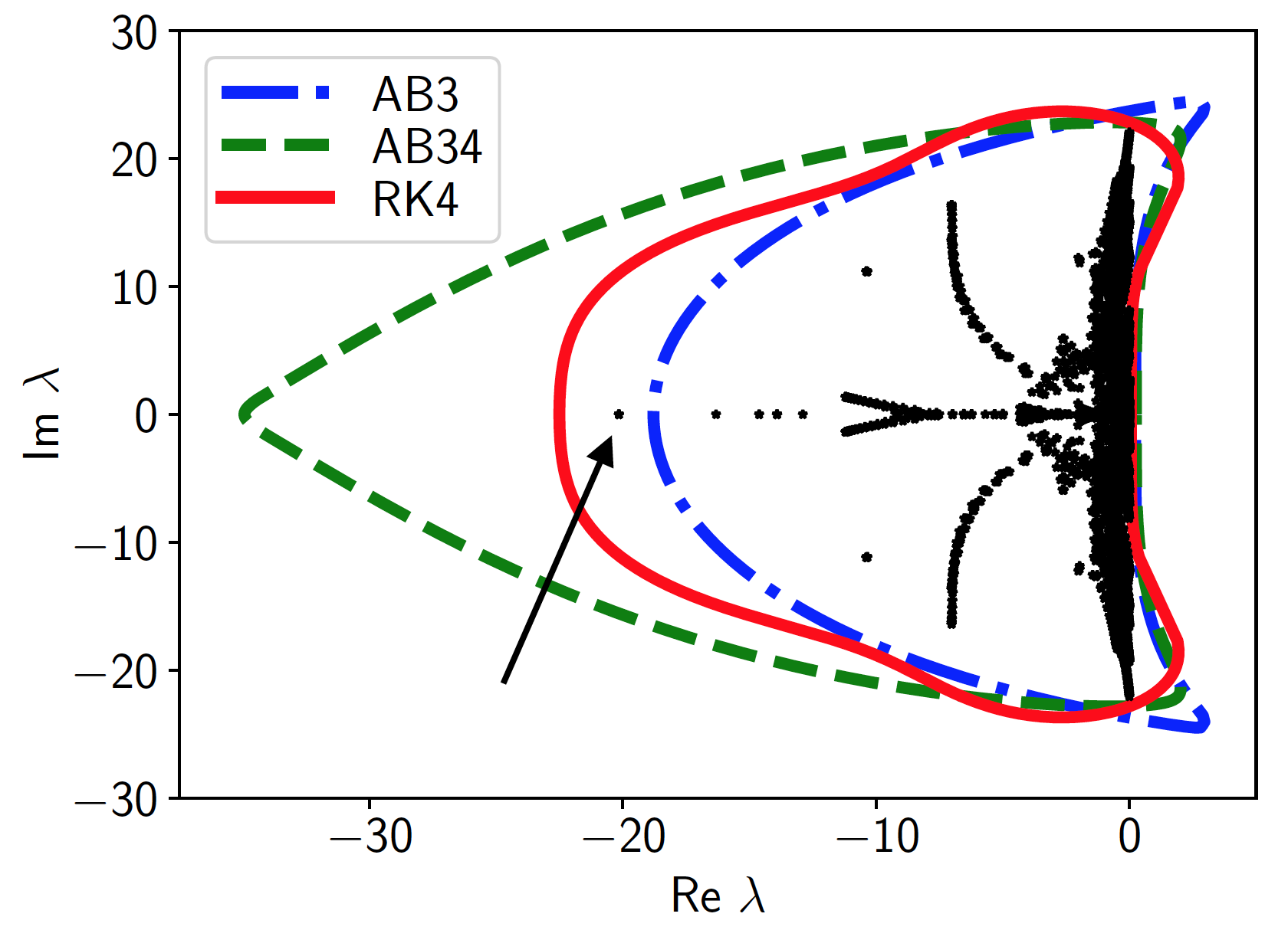
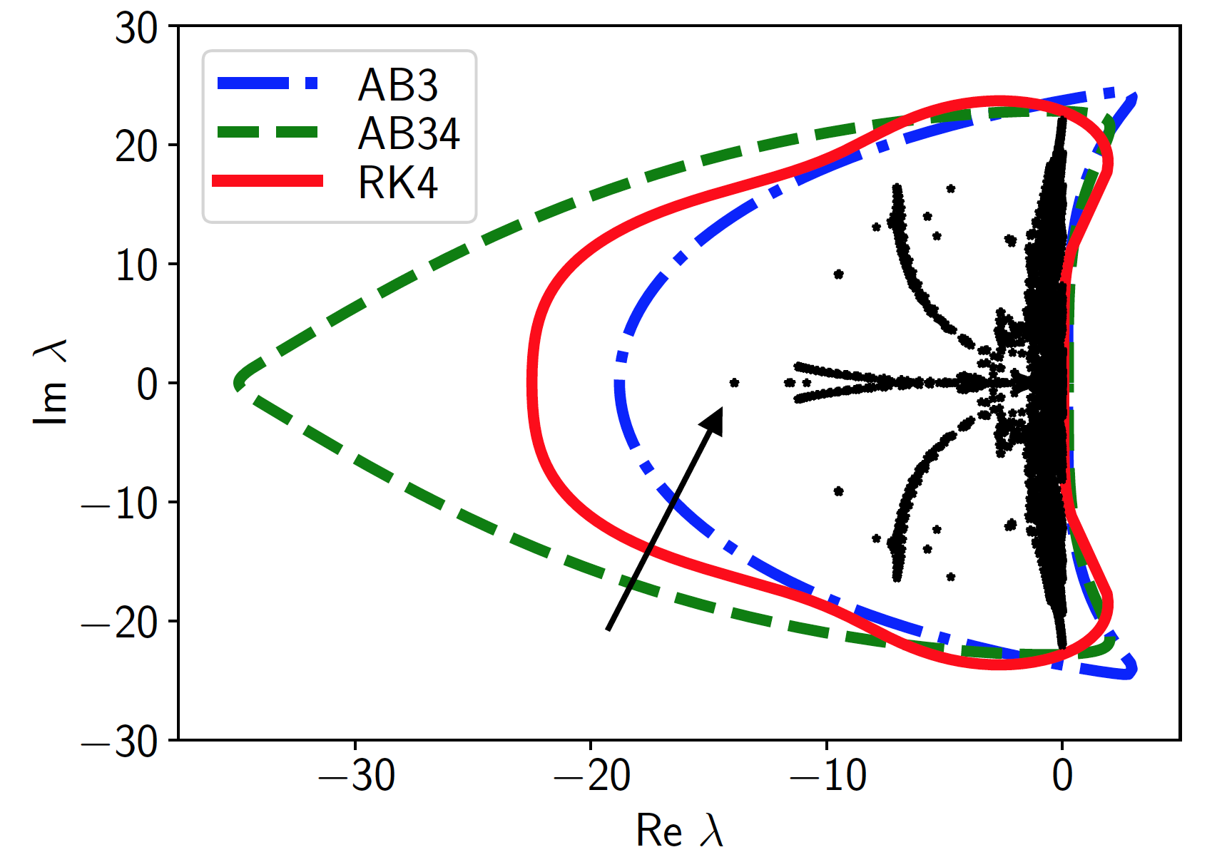
This method can be extended to any order and any number of additional history nodes. For third and fourth-order, the method produces what we term AB34 (third-order) and AB45 (fourth-order) schemes. Figures 2 and 3 plot stability regions (using the method we describe in B) for the new AB34 and AB35 schemes for comparison against a fourth-order Runge-Kutta (RK4) integrator and standard AB3 integrators and, similarly, of the new AB45 and AB46 schemes compared to RK4 and fourth-order Adams-Bashforth (AB4) integrators. Motivated by the amount of computational work per timestep, we normalize the approximate stability regions based on the number of right-hand side evaluations per timestep a given integrator requires — that is, while RK4 requires four right-hand side evaluations per timestep, Adams-Bashforth integrators only require one.
When compared with the approximate stability regions for standard Adams-Bashforth schemes, the approximate stability regions for the AB34 and AB45 schemes extend further along the negative real axis, while slightly shrinking along the imaginary axis. In the upcoming section, we will see that the SBP-SAT discretization we use motivates the use of this scheme to handle eigenvalues associated with inter-grid fluxes and, in the results section, we will therefore consider both the standard AB schemes (AB3, AB4) and the new AB34 and AB45 schemes in our analysis of convergence, stability, and performance considerations. While we will limit our continued discussion of extended-history schemes to AB34 and AB45 integrators, we can also extend the history used to produce the coefficients even further, creating AB35 and AB46 schemes, and again viewing normalized approximate stability regions for these schemes (Figures 2(b) and 3(b)).
3.3 Multi-rate Adams-Bashforth Integration
We now describe a multi-rate generalization of the scheme, making use of the algorithm introduced in [19]. We consider the following model system with “fast” and “slow” solution components:
With this in mind, we can set a slow (larger) time step for such that we maintain stability in the integration of the slow component. We also set a fast time step for such that is an integer multiple of , and define the ratio between the two, , assumed to be an integer, as the step ratio of the MRAB scheme. While the results presented here make use of only two separate state components, each with its own right-hand side function and independent rate, the approach is readily extensible to any number of rates.
In the two-component overset formulation with which we are concerned, we define the fast and slow components of our Navier-Stokes solution as the conserved variables on each grid, that is (using a two-grid case as an example): , , where the subscripts of the vectors indicate global grid number. We assume Grid 1 to be the grid with the fast-moving component of the solution, be it due to physical behavior or finer mesh spacing. Each right-hand side function and is a function of both the slow and fast states and — this coupling between the right-hand side functions is, in the case of our application of this theory to overset meshes, realized by the SAT penalty interpolation discussed in Section 2.2.
Within this two-component scheme, a few design choices are available:
- •
The order in which we evaluate and advance the solution components. Namely, two primary options are advancing the fast-evolving solution component through all of its micro-timesteps and waiting to perform the single macro-timestep required for the slow component until the end (a “fastest-first” scheme, per the nomenclature of [19]), or pursuing an algorithm in which the slow component is instead advanced first.
- •
For slowest-first evaluation schemes, the choice of whether or not to re-extrapolate the slow state after additional state and right-hand side information is gathered at the micro-timestep level.
Empirical observations on the effects of these choices are made in [29]. It is useful to step through a brief example of a multi-rate Adams-Bashforth integrator, using a system with a fast component requiring twice as many timesteps as the slow component to remain well-resolved (). We lay out the steps of a third-order fastest-first MRAB scheme with no re-extrapolation, assuming that evolves at the slow rate (macro-timestep ) and evolves at the fast rate (micro-timestep ). denotes extrapolants of the right-hand side functions as polynomial functions of both the set of time history points and the set of history values : , where
These polynomials approximating the evolution of and in time are what we will integrate to march and , and they will be updated to replace older history values with new right-hand side evaluations during the course of integration through a macro-timestep . We assume availability of right-hand side histories to start the AB method.
- Step 1:
Form the polynomial extrapolants we will integrate, per the AB methods described in Section 3.1:
The right-hand side history values of (used to form ) have been obtained at time points , , and current time , whereas the right-hand side history values of (used to form ) have been obtained at time points , , and . The macro-timestep can change on a per-macrostep basis, with the micro-timestep defined such that .
- Step 2:
March both and to time by integrating the polynomial extrapolants and formed in Step 1:
This results in a set of intermediate values and .
- Step 3:
Evaluate the fast right-hand side .
- Step 4:
Update the set of right-hand side history values for to include these new values, and construct a new extrapolant :
- Step 5:
March to time by integrating the extrapolant formed in Step 1:
- Step 6:
March to time by integrating the extrapolant formed in Step 3:
- Step 7:
Go to Step 1.
The scheme evaluates the fast-evolving right-hand side twice per macro-timestep , whereas the slowly-evolving right-hand side is only evaluated once. For the results shown later, this is the scheme we will use, albeit generalized to different step ratios .
4 Time Integration in SBP-SAT Discretizations
One of the critical questions to be answered is at what timestep sizes and the integrators developed in Section 3 remain stable. This section establishes the procedures and tools for characterizing the stability of the integrators developed in Section 3 in the context of the SBP-SAT discretization used.
4.1 Timestep Calculation
For the discretization of the Navier-Stokes equations described in Section 2, we will incorporate the metrics and multidimensionality into calculation of the timestep used by a given integrator. The maximum stable timestep for a given Navier-Stokes simulation using the SBP-SAT discretization is approximated via the following steps. First, we calculate an inviscid timestep:
| (4.1) |
and a viscous timestep:
| (4.2) |
where the vector contains the Cartesian velocities, is the speed of sound, , is the Jacobian, is the number of spatial dimensions, and the terms are the metric terms described in [36]. To determine the timestep, we calculate and at each mesh point, then take
| (4.3) |
and take an additional minimum over all mesh points. This timestep calculation is described in more detail in [36].
4.2 SAT Interpolation Stability
We now undertake a brief parameter study to show that one of the stiffest right-hand side components limiting the timestep when solving the Navier-Stokes equations with the overset discretization involves the SAT penalty-based interpolation (discussed in Section 2.2). Specifically, we will show that penalty terms applied at fringe points with more than one nonzero characteristic direction (i.e. corner points) produce eigenvalues with large negative real part. To illustrate this phenomenon, we can linearize a computationally small Navier-Stokes problem (using the procedure for approximation of the Jacobian described in [41] to form the approximate linear operator of the system) employing SAT interpolation on overset meshes and analyze the spectrum of the resulting global operator.
We express the time evolution of a fringe corner point as
| (4.4) |
with denoting the Navier-Stokes right-hand side, and denoting the penalty terms applied by the SAT interpolation procedure described in Section 2.2 (the latter two terms in (2.1)). We introduce a parameter to change the magnitude of terms associated with the interpolation penalty applied at the corner fringe points, and determine the right-hand side modes associated with these terms.
As for the case to be analyzed, we select an inviscid application of overset grids to the Euler equations with periodic boundary conditions. The initial condition is an -momentum gradient of the form
with the -momentum set to 0 everywhere. The initial condition and grid layout for this case are shown in Figure 4. Grid 1 (31 = 961 points) spans , , while Grid 2 ( = 1681 points) spans , .


We form the approximate linearized operators for this case for two values of the corner penalty weight parameter : and . By finding the eigenvalues of the two operators and comparing them, we can empirically identify the eigenvalues associated with the corners. Based on the highest-magnitude corner-associated eigenvalue that can be determined from comparing these spectra, it is clear that the approximate stability region of the RK4 scheme contains the corner-associated eigenvalue, which extends outwards along the negative real axis as we increase the penalty weight from 0.5 to 1, whereas the approximate stability region for the third-order AB scheme does not, where in each case the time step was calculated according to 4.3, and in which the scaling is controlled by the behavior along the imaginary axis in the situation considered. This motivated the development of the extended-history schemes discussed in Section 3.2, which are shown to improve the stability of AB schemes along the negative real axis. Figure 5 shows that the approximate stability region for the third-order extended-history AB scheme indeed contains the corner-associated eigenvalue.
4.3 Procedure for Determining Discrete Stability
We now develop a procedure for characterizing the discrete temporal stability of a given integrator within the SBP-SAT discretization using the same step matrix formulation as in the analysis of Section 3.2. We can express integration forward one timestep as a matrix operation on the integrator state vector :
| (4.5) |
where denotes the “step matrix” for a given integrator. These step matrices are functions of the timestep used in the simulation, and are formed using a linearization procedure that approximates the full Jacobian matrix of the system using finite differences. In doing so, analyzing the eigenvalues of this step matrix is analogous to analyzing the amplification factors of various modes in the global error of the scheme.
To construct the matrix , we first use an initial state as input to an integrator with timestep to march one step forward in time and form the base result about which we linearize. Next, we perturb a single element of the initial state vector using a small value . Using this perturbed state as an input to the integrator returns a state that — when compared to the base result — demonstrates the effect of the perturbation of that single element on the entire domain. If we define as a column vector with all zeroes except for a 1 in the th row, we can write
Thus we calculate the th column of the step matrix by perturbing the th initial state vector element, giving this modified initial state to the integrator to obtain , and taking
| (4.6) |
Note also that in the case of Adams-Bashforth integration, the stability vector element being perturbed may also be a right-hand side history element. For our perturbation , we use a value of . This procedure is similar to the Navier-Stokes linearization for SBP-SAT discretizations described in [41].
Once the matrix is formed, we consider the system discretely stable if the spectral radius fulfills the property . Therefore, creating step matrices for an integrator at a number of different values of will allow us to characterize that integrator’s stability. We use SLEPC [27] for the computation of the eigenvalues, using the default Krylov-Schur solver with a tolerance of . We use this procedure to determine the maximum stable timesteps of our integrators reported in Section 5.2.
4.4 Validation of the approximate stability calculation via RK4
We validate the procedure of the previous section by using it to determine the maximum stable timestep for an explicit fourth-order Runge-Kutta (RK4) integrator applied to 1D advection with a wave speed of 1. With a spatial domain with 61 mesh points, the step matrix analysis described in Section 4.3 predicts a maximum stable timestep for this case between and . Using the method described in B to approximate a given integrator’s stability region in the complex plane, we see that the imaginary-axis bound for an RK4 integrator is about . When using a fourth-order SBP operator as described in [58, 11, 38] for spatial discretization of the semidiscrete problem, and with periodic boundaries, the eigenvalues can be found analytically, and all lie on the imaginary axis, with a maximum eigenvalue of (a result given by Lele [35]). We can thus estimate the maximum stable timestep for this problem, noting a grid spacing of , to be , a result which is consistent with that of our step matrix procedure.
5 Numerical Results
5.1 Guiding Experiment: Viscous Flow Past a Cylinder
We consider two-dimensional viscous flow over a cylinder with diameter in the spatial domain . The cylinder center is located at , . The free-stream Mach number is 0.2, the Reynolds number is 200 and the Prandtl number is 0.72. We start our simulations from a steady state solution obtained after 100 non-dimensional time units (, using the nondimensionalization of [42]) using an RK4 integration scheme. Note that the timesteps we report are also non-dimensional. The physical problem is modeled using two overset meshes: a coarser, base Cartesian grid (), and a finer teardrop-shaped curvilinear grid () surrounding the stationary cylinder.

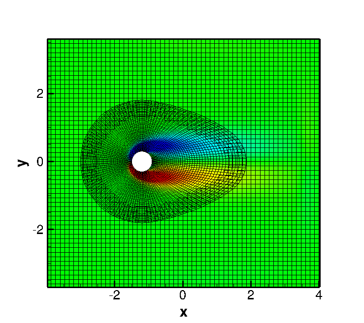
It is important to characterize the disparity in allowable timestep sizes such that we can estimate the maximum allowable step ratio SR we are able to use in our integrators. Calculated using the method of (4.1), (4.2), and (4.3), we find the ratio between the maximum timesteps on each grid to be about 12.
The boundary conditions employed in our simulation are as follows: The inner fine grid (Grid 2) is periodic in the azimuthal direction. We model the cylinder surface as an SAT isothermal wall per [61] (Equation 19). On Grid 1 (Cartesian base grid), all outer boundaries are modeled as SAT far-field following the procedure of [63] (Equation 22). In addition, sponge boundaries with a cell depth of 6 are used as described in [8] (Equation 69).
5.2 Multi-rate Adams-Bashforth Stability
We will now determine the stability characteristics of a given MRAB integrator by defining two ratios: and , where is the maximum stable timestep of the integrator in question, and and are the maximum stable timesteps for single-rate Adams-Bashforth (SRAB) and RK4 integrators, respectively, determined using the method of Section 4.3. Recall that the step ratio of a given MRAB integrator is given as , and is an integer value. An MRAB integrator with a step ratio of 1 is equivalent to an SRAB integrator. SR is a user-specified input.
For the experiments to determine stability, we set the value of the macro-timestep , build the step matrix of (4.5) (starting from a steady-state solution), and check for eigenvalues outside the unit disc, repeating the procedure until we find the maximum critical value of (to the nearest ) for an MRAB integrator with a given step ratio. The values are a measure of the maximum stable timesteps of these integrators relative to an RK4 integrator. The values reported for an MRAB integrator with a given order and history length use the maximum stable timestep for an SRAB integrator of the same order and history length. The percentages reported document percent efficiency of a given integrator, : that is, if an MRAB integrator with a step ratio of SR obtains an value of SR, it is deemed 100% efficient.
| Standard (AB3) | Extended-History (AB34) | ||||||||
|---|---|---|---|---|---|---|---|---|---|
| Int. | SR | % | % | ||||||
| RK4 | 0.0217 | 1.000 | 5.13 | 0.0217 | 1.000 | 3.86 | |||
| SRAB | 1 | 0.0042 | 0.195 | 1.00 | 100 | 0.0056 | 0.259 | 1.00 | 100 |
| MRAB | 2 | 0.0084 | 0.388 | 1.99 | 99.5 | 0.0113 | 0.518 | 2.00 | 100 |
| MRAB | 3 | 0.0127 | 0.583 | 2.99 | 99.7 | 0.0169 | 0.775 | 2.99 | 99.7 |
| MRAB | 4 | 0.0169 | 0.777 | 3.99 | 99.8 | 0.0225 | 1.035 | 3.99 | 99.8 |
| MRAB | 5 | 0.0171 | 0.788 | 4.04 | 80.8 | 0.0281 | 1.294 | 4.99 | 99.8 |
| MRAB | 6 | 0.0171 | 0.788 | 4.04 | 67.3 | 0.0282 | 1.296 | 5.00 | 83.3 |
| MRAB | 7 | 0.0171 | 0.788 | 4.04 | 57.7 | 0.0282 | 1.296 | 5.00 | 71.4 |
| MRAB | 8 | 0.0171 | 0.788 | 4.04 | 50.5 | 0.0282 | 1.296 | 5.00 | 62.5 |
| MRAB | 9 | 0.0171 | 0.788 | 4.04 | 44.9 | 0.0282 | 1.296 | 5.00 | 55.6 |
| MRAB | 10 | 0.0171 | 0.788 | 4.04 | 40.4 | 0.0282 | 1.296 | 5.00 | 50.0 |
| MRAB | 20 | 0.0171 | 0.788 | 4.04 | 20.2 | 0.0282 | 1.296 | 5.00 | 25.0 |
| Standard (AB4) | Extended-History (AB45) | ||||||||
|---|---|---|---|---|---|---|---|---|---|
| Int. | SR | % | % | ||||||
| RK4 | 0.0217 | 1.000 | 9.42 | 0.0217 | 1.000 | 5.63 | |||
| SRAB | 1 | 0.0023 | 0.106 | 1.00 | 100 | 0.0039 | 0.178 | 1.00 | 100 |
| MRAB | 2 | 0.0046 | 0.212 | 2.00 | 100 | 0.0078 | 0.356 | 2.00 | 100 |
| MRAB | 3 | 0.0070 | 0.321 | 3.02 | 100 | 0.0116 | 0.533 | 3.00 | 100 |
| MRAB | 4 | 0.0093 | 0.427 | 4.02 | 100 | 0.0155 | 0.711 | 4.00 | 100 |
| MRAB | 5 | 0.0093 | 0.430 | 4.05 | 81.0 | 0.0180 | 0.827 | 4.65 | 93.0 |
| MRAB | 6 | 0.0093 | 0.430 | 4.05 | 67.5 | 0.0180 | 0.827 | 4.65 | 77.5 |
| MRAB | 7 | 0.0093 | 0.430 | 4.05 | 57.9 | 0.0180 | 0.827 | 4.65 | 66.4 |
| MRAB | 8 | 0.0093 | 0.430 | 4.05 | 50.6 | 0.0180 | 0.827 | 4.65 | 58.1 |
| MRAB | 9 | 0.0093 | 0.430 | 4.05 | 45.0 | 0.0180 | 0.827 | 4.65 | 51.7 |
| MRAB | 10 | 0.0093 | 0.430 | 4.05 | 40.5 | 0.0180 | 0.827 | 4.65 | 46.5 |
| MRAB | 20 | 0.0093 | 0.430 | 4.05 | 20.3 | 0.0180 | 0.827 | 4.65 | 23.3 |
The results of Tables 1 and 2 show that the extended-history schemes have higher maximum stable timesteps than their standard counterparts of same order. All schemes attain near-perfect efficiency () for SR-values up to about a third of the speed ratio of 12 for this case (), with the extended-history schemes maintaining this efficiency for the cases as well, a result due to the improved stability of these schemes along the negative real axis. Above this step ratio, we expect our performance to degrade, given that we are simply performing extra right-hand side evaluations (more micro-timesteps on the fast grid) with no commensurate macro-timestep gain. The increase from third to fourth order necessitates the use of lower timesteps for all step ratios, but the same qualitative ceiling as in the third-order case is observed. The third-order MRAB scheme with extended history is the only scheme able to attain for any step ratio, indicating maximum stable timesteps larger than that of the RK4 integrator.
5.3 Multi-Rate Adams-Bashforth Accuracy and Convergence
We now examine the accuracy of the MRAB schemes and confirm that they are convergent. In presenting accuracy results for our schemes, we will examine integrators for values of SR ranging from 2 to 6. As we have seen in the previous section, above this step ratio, the maximum stable timestep remains unchanged for all AB integrators for our speed ratio of about 12. For each integrator, we calculate an estimated order of convergence (EOC) using 3 data points consisting of the macro-timestep used and the maximum error obtained in the density after 2.5 NDTU. The initial condition for these 2.5-NDTU integrations is a uniform subsonic flow with Mach number in the -direction (before the boundary layer has developed on the cylinder), and the true solution to which the solution obtained with our integrators is compared to form the error is the solution obtained using an RK4 integrator with a timestep of . Based on the stability results of Section 5.2, we limit our convergence study to the third-order schemes, which have the highest potential to improve performance. We see in Table 4 that an estimated order of convergence of about 3 is obtained in all cases, as expected.
| SR | err, | err, | err, | EOC |
|---|---|---|---|---|
| 2 | 1.93E-06 | 1.79E-08 | 2.44E-09 | 2.900 |
| 3 | 1.73E-06 | 1.48E-08 | 1.87E-09 | 2.965 |
| 4 | 1.68E-06 | 1.40E-08 | 1.77E-09 | 2.977 |
| 5 | 1.67E-06 | 1.38E-08 | 1.73E-09 | 2.984 |
| 6 | 1.66E-06 | 1.37E-08 | 1.71E-09 | 2.986 |
| SR | err, | err, | err, | EOC |
|---|---|---|---|---|
| 2 | 3.56E-06 | 3.42E-08 | 4.53E-09 | 2.894 |
| 3 | 3.29E-06 | 2.86E-08 | 3.63E-09 | 2.956 |
| 4 | 3.23E-06 | 2.73E-08 | 3.44E-09 | 2.971 |
| 5 | 3.22E-06 | 2.68E-08 | 3.37E-09 | 2.979 |
| 6 | 3.21E-06 | 2.66E-08 | 3.34E-09 | 2.982 |
6 MRAB Performance
6.1 Performance Model
Our next task is to characterize the benefit in performance when using these multi-rate integrators. What expectations should we have in terms of the reduction in computational work required for these new schemes compared to single-rate schemes?
To answer this question, we will develop a performance model of how we would expect an MRAB integrator of a certain step ratio to perform in comparison to the same RK4 integrator used as a baseline for the accuracy and stability tests. In doing so, we make a few assumptions: we assume that right-hand side evaluations make up the bulk of the computational cost of the Navier-Stokes simulation, and we also assume that all simulations will be performed at or near the maximum stable timestep of a given integrator.
We note in forming this model that in a given timestep for an RK4 integrator, four right-hand side evaluations must be performed, whereas in the AB schemes, only one evaluation is needed. Thus, to reach time , we can write expressions for the total number of right-hand side evaluations each integrator will need to perform:
| (6.1) | |||
| (6.2) |
In (6.1) and (6.2), is the number of points on the fast grid, and is the number of points on the slow grid (assuming a two-grid configuration). Furthermore, SR is the step ratio of the AB integrator (the number of micro-steps taken on the fast grid per macro-step on the slow grid — for an SRAB integrator, ), is the timestep taken by the RK4 scheme, and is the end time to be reached. Recall that the factor is defined in Section 5.2 as
This factor relates to the timestep restrictions of AB integrators relative to RK4. These restrictions, as we have seen in the analyses of Section 5.2, are imposed by stability constraints. Namely, the maximum stable timestep of the RK4 integrator applied to a certain case will be larger than that of an AB integrator, and therefore more timesteps must be taken with an AB integrator to reach time than the RK4 integrator takes to reach time .
Given the assumptions of our performance model, calculating the percent reduction in right-hand side evaluations therefore provides a theoretical estimate of computational work saved when using a given AB integrator. We define the resulting speedup as
| (6.3) |
Using this definition, any values of SU over 1 indicate a profitable integrator, whereas values of 1 or less indicate equal or decreased performance. As an example of this performance model in execution, we can compose a model for the case discussed in Section 5.1 modeling the cylinder in crossflow, for a number of step ratios, and for both third and fourth order. We use the grid data presented in Section 5.1 and the values given in Section 5.2, and for simplicity we take . For these results and for all of the results that follow, we will use the more potentially profitable extended-history (AB34 and AB45) integrators.
| Integrator | Total RHS Evals | % Red. from RK4 | SU |
|---|---|---|---|
| RK4 | 34244 | 0.00 | 1.00 |
| SRAB () | 33023 | 3.57 | 1.04 |
| MRAB () | 25846 | 24.52 | 1.32 |
| MRAB () | 23529 | 31.29 | 1.46 |
| MRAB () | 22310 | 34.85 | 1.53 |
| MRAB () | 21581 | 36.98 | 1.59 |
| MRAB () | 25274 | 26.19 | 1.35 |
| Integrator | Total RHS Evals | % Red. from RK4 | SU |
|---|---|---|---|
| RK4 | 34244 | 0.00 | 1.00 |
| SRAB () | 48154 | 40.62 | 0.71 |
| MRAB () | 37694 | 10.08 | 0.91 |
| MRAB () | 34204 | 0.12 | 1.00 |
| MRAB () | 32459 | 5.21 | 1.05 |
| MRAB () | 33756 | 1.42 | 1.01 |
| MRAB () | 39608 | 15.66 | 0.86 |
Table 5 shows that we can expect speedup for all third-order MRAB integrators using the extended history scheme for this specific case — however, based on Table 6, we speculate that fourth-order MRAB integrators using the extended histories will largely fail to be profitable for this specific case, though the fourth-order schemes do reach a break-even point at , attaining very minimal performance benefit at (around 5% reduction in right-hand side evaluations), before decreasing again due to the stability ceiling observed in Section 5.2.
6.2 Sequential Performance
Having developed a performance model in the previous subsection and thus obtained expectations for how the integrators should perform, we now develop tests to verify this model. We gauge performance by using a given integrator to march the viscous flow over a cylinder case for 10 NDTU (again, starting from a steady state solution) at the maximum stable timestep of the integrator, measuring end-to-end wall clock time of the Navier-Stokes solver, time spent calculating right-hand sides, time spent performing the necessary interpolations between grids and time spent performing spatial operator-related tasks, a subset of the right-hand side calculation. We limit our performance testing here to third-order MRAB integrators with the extended history scheme only, as Section 6.1 shows these to be the most promising for this case. The percentages reported for each step ratio document the percent reduction in time compared to that of the RK4 integrator, and the predicted percentage is that which results from the performance model (based purely on right-hand side evaluations as given by (6.1) and (6.2)).
| Int. | R [s] | % | O [s] | % | I [s] | % | E [s] | % | % Pred. |
|---|---|---|---|---|---|---|---|---|---|
| RK4 | 29.9 | 18.4 | 0.623 | 38.7 | |||||
| () | 28.29 | 5.6 | 17.44 | 5.2 | 0.273 | 56.2 | 41.73 | 8.0 | 3.6 |
| () | 22.76 | 23.9 | 14.07 | 23.5 | 0.214 | 65.7 | 30.14 | 22.0 | 24.5 |
| () | 21.60 | 27.7 | 13.33 | 27.5 | 0.201 | 67.7 | 28.90 | 25.2 | 31.3 |
| () | 20.91 | 30.0 | 12.91 | 29.8 | 0.194 | 68.9 | 27.50 | 28.9 | 34.9 |
| () | 18.13 | 39.3 | 11.17 | 39.2 | 0.163 | 73.8 | 23.60 | 38.9 | 37.0 |
| () | 20.27 | 32.2 | 12.51 | 32.0 | 0.182 | 70.8 | 24.13 | 37.6 | 26.2 |
We see in Table 7 that the measured times given for our new SRAB and MRAB integrators are all lower than those of RK4, with one exception (the SRAB integrator has a slightly larger end-to-end time). Furthermore, we note in the case of sequential performance profiling that the observed interpolation times are low as we would expect (when not running the solver in parallel, this amounts to copying data between buffers) — we will see that the time spent interpolating becomes more significant as we transition to a discussion of parallel runs. Regarding the percentages, while we see good agreement with the overall trend of the model of Section 6.1, we see that a number of the percentage reductions observed are slightly lower than those predicted by the model.
6.3 Parallel Performance
In this section, we perform tests similar to those of Section 6.2, with a specific focus on the distributed-memory parallelization of the new integrators, in order to answer the question of how communication and interpolation between grids affects performance. The procedure with these tests is the same as in Section 6.2, but an important distinction to note is that we document end-to-end wall clock time, but the times reported for right-hand side calculations, operator tasks, and interpolation are accumulated inclusive times (the total time spent by all processors performing these specific tasks). In the tables that follow, we report times for third-order MRAB integrators with extended history for various step ratios. Bold values indicate lower time spent with a certain task than that of the RK4 integrator.
| Proc | RK4 | % | % | % | % | ||||
|---|---|---|---|---|---|---|---|---|---|
| 2 | 23.52 | 25.21 | 7.2 | 33.82 | 43.8 | 25.70 | 9.3 | 24.28 | 3.2 |
| 4 | 17.12 | 19.49 | 13.8 | 10.04 | 41.4 | 8.80 | 48.6 | 10.05 | 41.3 |
| 8 | 8.37 | 9.36 | 11.9 | 6.41 | 23.4 | 6.64 | 20.6 | 7.04 | 15.8 |
| 16 | 4.98 | 5.50 | 10.4 | 3.93 | 21.1 | 3.91 | 21.5 | 4.50 | 9.6 |
| Proc | RK4 | % | % | % | % | ||||
|---|---|---|---|---|---|---|---|---|---|
| 2 | 31.17 | 29.82 | 4.3 | 23.67 | 24.1 | 20.91 | 32.9 | 20.66 | 33.7 |
| 4 | 35.26 | 33.40 | 5.3 | 27.07 | 23.2 | 24.12 | 31.6 | 26.62 | 24.5 |
| 8 | 44.28 | 41.97 | 5.2 | 32.97 | 25.5 | 28.06 | 36.6 | 31.74 | 28.3 |
| 16 | 53.36 | 48.82 | 8.5 | 39.81 | 25.4 | 34.30 | 35.7 | 38.97 | 27.0 |
| Proc | RK4 | % | % | % | % | ||||
|---|---|---|---|---|---|---|---|---|---|
| 2 | 19.17 | 18.46 | 3.7 | 14.61 | 23.8 | 12.86 | 32.9 | 12.65 | 34.0 |
| 4 | 20.97 | 20.12 | 4.1 | 16.37 | 21.9 | 14.63 | 30.2 | 15.78 | 24.7 |
| 8 | 24.97 | 23.83 | 4.6 | 18.88 | 24.4 | 16.29 | 34.8 | 18.60 | 25.5 |
| 16 | 28.52 | 27.00 | 5.3 | 21.71 | 23.9 | 18.29 | 35.9 | 21.42 | 24.9 |
| Proc | RK4 | % | % | % | % | ||||
|---|---|---|---|---|---|---|---|---|---|
| 2 | 5.55 | 3.86 | 30.5 | 29.61 | 433.5 | 21.92 | 295.0 | 22.04 | 297.1 |
| 4 | 24.54 | 21.02 | 14.3 | 3.73 | 84.8 | 2.28 | 90.7 | 5.03 | 79.5 |
| 8 | 13.27 | 10.05 | 24.3 | 1.46 | 89.0 | 6.60 | 50.3 | 11.31 | 14.8 |
| 16 | 15.45 | 12.12 | 21.6 | 1.93 | 87.5 | 8.53 | 44.8 | 14.54 | 5.9 |
Generally, what we see here is first and foremost that the time spent on right-hand side and operator-related tasks (Table 9 and Table 10, respectively) is always lowered by the use of multi-rate methods, in certain cases by over 30%, in line with the model of Section 6.1). Furthermore, the end-to-end wall clock times (Table 8) largely show that the reduction in right-hand side evaluations indeed leads to end-to-end speedup for a number of step ratios and processor counts. Regarding the SRAB scheme (), we see that the times spent in the interpolation, operator, and right-hand side tasks are all lower than those of RK4, yet the end-to-end times are very slightly higher for all core counts. The reason for this is the introduction of higher overhead from elsewhere in the program due to the requirement that more timesteps be run to reach the same end time.
For tests using 2 processors, we see a large amount of time spent in interpolation subroutines for all multi-rate integrators. This is due to the fact that the usage of multi-rate integration in the overset sense induces load imbalance within the application, given that in a given macro-timestep, we will be evaluating more right-hand sides on certain grids than on others. This causes long processor wait times (accounted for, in our case, as interpolation time) due to suboptimal work distribution and motivates a change to the existing decomposition of the problem, which simply distributes processors to grids based on the ratio of that grid’s number of points to the total number of points in the simulation. Rescaling this decomposition based on the multi-rate step ratio being used (a direct indication of how many right-hand side evaluations per macro-timestep a given processor is responsible for) allows us to produce improved performance results at higher processor counts, reducing the wait times spent in grid-to-grid communication. With only two cores, however, we are unable to rescale the decomposition to improve the load imbalance produced by multi-rate. Further effects of inter-grid communications are shown in the next section, focusing on large-scale results.
6.4 Large-Scale Performance
We now move to a different example to investigate the performance of the integrators at larger scale. The grids for this new case, modeling ignition via laser-induced breakdown (LIB) of an underexpanded jet, are shown in Figure 7, and are numerically described in Table 12. Note the percentage of total points in Grid 1 — this will be our fast grid, while the remaining 3 grids will be the slow grids (see Figure 8).
| Grid | Grid Type | No. of Points | % of Total |
|---|---|---|---|
| 1 | Cartesian | 12,582,912 | 47.7 |
| 2 | Cylindrical | 339,521 | 1.3 |
| 3 | Cylindrical | 11,419,614 | 43.3 |
| 4 | Cylindrical | 2,060,250 | 7.8 |


Using the performance model outlined in (6.1), (6.2), and (6.3), and assuming values for this case similar to the viscous flow over a cylinder case, we can calculate expected performance. We test step ratios from 1 to 5, as we have seen in Section 5.2 that this is the range of step ratios for which we maintain perfect efficiency ().
| Integrator | Total RHS Evals | % Red. from RK4 | SU |
|---|---|---|---|
| RK4 | 105,609,188 | 0.00 | 1.00 |
| SRAB | 101,939,371 | 3.50 | 1.04 |
| MRAB () | 75,261,021 | 26.5 | 1.36 |
| MRAB () | 66,539,511 | 37.0 | 1.59 |
| MRAB () | 62,011,632 | 41.3 | 1.70 |
| MRAB () | 59,299,803 | 43.8 | 1.78 |
The results in Table 13 suggest that we should expect moderate speedup when using a third-order multi-rate scheme with , with the speedup increasing as we increase the step ratio to 5. Performing the integration using these schemes allows us to measure the same times of interest as in the previous section and compare them with this model. The results we present are obtained from a 6,144-core simulation on Stampede2, an NSF-supported supercomputer at the University of Texas and the Texas Advanced Computing Center (TACC), and report scaled time spent in various portions of the Navier-Stokes solver relative to the end-to-end wall clock time of a Runge-Kutta-driven simulation.
These results show measured times that correlate well with what we would expect for reduction in operator and right-hand side costs, and furthermore, we see large reductions in the time spent in interpolation-related subroutines for all step ratios — this is a direct result of implementation of multi-rate-specific overset interpolation schemes featuring selective communications and separate send-receive schemes (interleaved with right-hand side calculation). In the end, the main time marching loop sees moderate speedup for all step ratios above 1, but is below the prediction of the performance model. Our results show roughly constant time spent in all other components of the Navier-Stokes solver not explicitly timed, and higher multi-rate times in two specific portions of the solver, both of which can be readily explained:
- •
Timestep calculation. While we do scale the frequency of these calculations such that they occur the same number of times in RK4 as in our integrators, the aforementioned new interpolation scheme — which reduces the amount of wait times in inter-grid communication — shifts load imbalance to these calculations, which feature communication between all processors to determine the minimum timestep.
- •
Ghost cell exchanges. These operations involve communication between processors working on the same grid (to exchange ghost cell data used to fill boundary stencils). Rescaling the decomposition the solver uses to allocate more processing power to the fast grid and account for the inherent load imbalance (as mentioned at the end of Section 6.3) results in more processor boundaries that require this operation to be performed. The question of balancing inter-grid communication with intra-grid communication when decomposing the problem to avoid load imbalance remains. We leave this for future work.
In short, the results for this large-scale case show that while we see a performance benefit due to decrease in right-hand side evaluations and implementation of more efficient interpolation routines, the improvement is below the estimates of the performance model due to increased communication times induced by load imbalance.
7 Conclusions and Future Work
In this paper, we have developed multi-rate Adams-Bashforth integrators to take advantage of an overset discretization of the Navier-Stokes equations using SBP spatial operators, SAT boundary conditions, and an SAT penalty-based interpolation method. We improve the temporal stability of these integrators by introducing extended-history Adams-Bashforth schemes with higher maximum stable timesteps for ODE systems with eigenvalues along the negative real axis. These new schemes are shown, using a number of numerical tools and examples, to be stable and accurate, and are also shown to improve performance and reduce the computational work required to march a given system in time when compared to both single-rate Adams-Bashforth integrators and a fourth-order Runge-Kutta integrator. A simple performance model is also developed (see Equations (6.1), (6.2), and (6.3)) that shows the dependence of expected speedup via the use of multi-rate Adams-Bashforth integration on both the allowable step ratio and the ratio of slow points to fast points. In particular, this model shows that performance benefit is maximized in cases where the ratio of slow points to fast points is high, and where the fast points have an evolutionary timescale significantly smaller than that of the slow points. In our demonstration of performance improvement using these new multi-rate schemes, we also identify load balance as a critical consideration for further reduction in computational time — this is left for future work.
Acknowledgments
This material is based in part upon work supported by the Department of Energy, National Nuclear Security Administration, under Award Number DE-NA0002374 and by the National Science Foundation under grant number CCF-1524433. Computational support has been provided, in part, by the National Science Foundation XSEDE resources under grant TG-CTS090004.
References
- [1] J. Andrus. Stability of a multi-rate method for numerical integration of ode’s. Computers & Mathematics with Applications, 25(2):3–14, 1993.
- [2] J. F. Andrus. Numerical solution of systems of ordinary differential equations separated into subsystems. SIAM Journal on Numerical Analysis, 16(4):605–611, 1979.
- [3] F. Bashforth and J. C. Adams. An attempt to test the theories of capillary action. University Press, 1883.
- [4] J. Bell, M. Berger, J. Saltzman, and M. Welcome. Three-dimensional adaptive mesh refinement for hyperbolic conservation laws. SIAM Journal on Scientific Computing, 15(1):127–138, 1994.
- [5] J. Benek, J. Steger, and F. C. Dougherty. A flexible grid embedding technique with application to the Euler equations. In 6th Computational Fluid Dynamics Conference Danvers, page 1944, 1983.
- [6] M. J. Berger and P. Colella. Local adaptive mesh refinement for shock hydrodynamics. Journal of Computational Physics, 82(1):64–84, 1989.
- [7] M. J. Berger and J. Oliger. Adaptive mesh refinement for hyperbolic partial differential equations. Journal of Computational Physics, 53(3):484–512, 1984.
- [8] D. J. Bodony. Analysis of sponge zones for computational fluid mechanics. Journal of Computational Physics, 212(2):681–702, 2006.
- [9] D. J. Bodony. Accuracy of the simultaneous-approximation-term boundary condition for time-dependent problems. Journal of Scientific Computing, 43(1):118–133, 2010.
- [10] D. J. Bodony, G. Zagaris, A. Reichert, and Q. Zhang. Provably stable overset grid methods for computational aeroacoustics. Journal of Sound and Vibration, 330(17):4161–4179, 2011.
- [11] M. H. Carpenter, D. Gottlieb, and S. Abarbanel. Time-stable boundary conditions for finite-difference schemes solving hyperbolic systems: methodology and application to high-order compact schemes. Technical report, NASA, 1993.
- [12] G. Chesshire and W. D. Henshaw. Composite overlapping meshes for the solution of partial differential equations. Journal of Computational Physics, 90(1):1–64, 1990.
- [13] G. Chesshire and W. D. Henshaw. A scheme for conservative interpolation on overlapping grids. SIAM Journal on Scientific Computing, 15(4):819–845, 1994.
- [14] H. Chou and J. Ekaterinaris. A compact high-order CFD package for the flow solver OVERFLOW. In 41st Aerospace Sciences Meeting and Exhibit, page 1234, 2003.
- [15] E. M. Constantinescu and A. Sandu. Multirate timestepping methods for hyperbolic conservation laws. Journal of Scientific Computing, 33(3):239–278, 2007.
- [16] C. Dawson and R. Kirby. High resolution schemes for conservation laws with locally varying time steps. SIAM Journal on Scientific Computing, 22(6):2256–2281, 2001.
- [17] C. Engstler and C. Lubich. Multirate extrapolation methods for differential equations with different time scales. Computing, 58(2):173–185, 1997.
- [18] C. Gear. Multirate methods for ordinary differential equations. Technical report, Illinois Univ., Urbana (USA). Dept. of Computer Science, 1974.
- [19] C. W. Gear and D. Wells. Multirate linear multistep methods. BIT Numerical Mathematics, 24(4):484–502, 1984.
- [20] M. Günther and P. Rentrop. Multirate ROW methods and latency of electric circuits. Applied Numerical Mathematics, 13(1):83–102, 1993.
- [21] M. Günther, A. Kværnø, and P. Rentrop. Multirate partitioned Runge-Kutta methods. BIT Numerical Mathematics, 41(3):504–514, 2001.
- [22] B. Gustafsson. The convergence rate for difference approximations to mixed initial boundary value problems. Mathematics of Computation, 29(130):396–406, 1975.
- [23] B. Gustafsson. The convergence rate for difference approximations to general mixed initial-boundary value problems. SIAM Journal on Numerical Analysis, 18(2):179–190, 1981.
- [24] B. Gustafsson, H.-O. Kreiss, and J. Oliger. Time dependent problems and difference methods, volume 24. John Wiley & Sons, 1995.
- [25] W. D. Henshaw. A high-order accurate parallel solver for Maxwell’s equations on overlapping grids. SIAM Journal on Scientific Computing, 28(5):1730–1765, 2006.
- [26] W. D. Henshaw and K. K. Chand. A composite grid solver for conjugate heat transfer in fluid–structure systems. Journal of Computational Physics, 228(10):3708–3741, 2009.
- [27] V. Hernandez, J. E. Roman, and V. Vidal. SLEPc: A scalable and flexible toolkit for the solution of eigenvalue problems. ACM Trans. Math. Software, 31(3):351–362, 2005.
- [28] K. Heun. Neue methoden zur approximativen integration der differentialgleichungen einer unabhängigen veränderlichen. Z. Math. Phys, 45:23–38, 1900.
- [29] A. Klöckner. High-performance high-order simulation of wave and plasma phenomena. PhD thesis, Brown University, 2010.
- [30] A. Klöckner and M. Wala. Dagrt. https://gitlab.tiker.net/inducer/dagrt, 2018a.
- [31] A. Klöckner and M. Wala. Leap. https://gitlab.tiker.net/inducer/leap, 2018b.
- [32] W. Kutta. Beitrag zur näherungweisen integration totaler differentialgleichungen. 1901.
- [33] A. Kværnø. Stability of multirate Runge-Kutta schemes. 2000.
- [34] Y. Lee and J. Baeder. High-order overset method for blade vortex interaction. In 40th AIAA Aerospace Sciences Meeting & Exhibit, page 559, 2002.
- [35] S. K. Lele. Compact finite difference schemes with spectral-like resolution. Journal of Computational Physics, 103(1):16–42, 1992.
- [36] R. W. MacCormack. Numerical computation of compressible and viscous flow. American Institute of Aeronautics and Astronautics, 2014.
- [37] R. Magnus and H. Yoshihara. Inviscid transonic flow over airfoils. AIAA Journal, 8(12):2157–2162, 1970.
- [38] K. Mattsson, M. Svärd, and J. Nordström. Stable and accurate artificial dissipation. Journal of Scientific Computing, 21(1):57–79, 2004.
- [39] R. Noack and J. Slotnick. A summary of the 2004 overset symposium on composite grids and solution technology. In 43rd AIAA Aerospace Sciences Meeting and Exhibit, page 921, 2005.
- [40] S. Osher and R. Sanders. Numerical approximations to nonlinear conservation laws with locally varying time and space grids. Mathematics of Computation, 41(164):321–336, 1983.
- [41] M. Osusky, J. Hicken, and D. Zingg. A parallel Newton-Krylov-Schur flow solver for the Navier-Stokes equations using the SBP-SAT approach. In 48th AIAA Aerospace Sciences Meeting Including the New Horizons Forum and Aerospace Exposition, page 116, 2010.
- [42] J. Park, K. Kwon, and H. Choi. Numerical solutions of flow past a circular cylinder at Reynolds numbers up to 160. KSME International Journal, 12(6):1200–1205, 1998.
- [43] A. Sandu and E. M. Constantinescu. Multirate explicit Adams methods for time integration of conservation laws. Journal of Scientific Computing, 38(2):229–249, 2009.
- [44] J. Sanz-Serna. Some aspects of the boundary locus method. BIT Numerical Mathematics, 20(1):97–101, 1980.
- [45] V. Savcenco, W. Hundsdorfer, and J. Verwer. A multirate time stepping strategy for stiff ordinary differential equations. BIT Numerical Mathematics, 47(1):137–155, 2007.
- [46] B. Seny, J. Lambrechts, R. Comblen, V. Legat, J.-F. Remacle, et al. Multirate time stepping methods for accelerating explicit discontinuous Galerkin computations. In 9th International Workshop on Multiscale (Un)-structured Mesh Numerical Modeling for Coastal, Shelf, and Global Ocean Dynamics, 2010.
- [47] B. Seny, J. Lambrechts, T. Toulorge, V. Legat, and J.-F. Remacle. An efficient parallel implementation of explicit multirate Runge–Kutta schemes for discontinuous Galerkin computations. Journal of Computational Physics, 256:135–160, 2014.
- [48] N. Sharan. Time-stable high-order finite difference methods for overset grids. PhD thesis, University of Illinois at Urbana-Champaign, 2016.
- [49] N. Sharan, C. Pantano, and D. J. Bodony. Time-stable overset grid method for hyperbolic problems using summation-by-parts operators. Journal of Computational Physics, 361:199–230, 2018.
- [50] S. Sherer and M. Visbal. Implicit large eddy simulations using a high-order overset grid solver. In 34th AIAA Fluid Dynamics Conference and Exhibit, page 2530, 2004.
- [51] S. Sherer, M. Visbal, and M. Galbraith. Automated preprocessing tools for use with a high-order overset-grid algorithm. In 44th AIAA Aerospace Sciences Meeting and Exhibit, page 1147, 2006.
- [52] S. E. Sherer and J. N. Scott. High-order compact finite-difference methods on general overset grids. Journal of Computational Physics, 210(2):459–496, 2005.
- [53] B. Sjogreen and H. Yee. Variable high order multiblock overlapping grid methods for mixed steady and unsteady multiscale viscous flows. Technical report, Lawrence Livermore National Lab.(LLNL), Livermore, CA (United States), 2007.
- [54] G. Starius. Composite mesh difference methods for elliptic boundary value problems. Numerische Mathematik, 28(2):243–258, 1977.
- [55] G. Starius. On composite mesh difference methods for hyperbolic differential equations. Numerische Mathematik, 35(3):241–255, 1980.
- [56] J. Steger. The Chimera method of flow simulation. In Workshop on Applied CFD, Univ of Tennessee Space Institute, volume 188, 1991.
- [57] A. Stock. Development and application of a multirate multistep AB method to a discontinuous Galerkin method based particle in cell scheme, 2009.
- [58] B. Strand. Summation by parts for finite difference approximations for d/dx. Journal of Computational Physics, 110(1):47–67, 1994.
- [59] N. Suhs, S. Rogers, and W. Dietz. PEGASUS 5: an automated pre-processor for overset-grid CFD. In 32nd AIAA Fluid Dynamics Conference and Exhibit, page 3186, 2002.
- [60] M. Svärd and J. Nordström. On the order of accuracy for difference approximations of initial-boundary value problems. Journal of Computational Physics, 218(1):333–352, 2006.
- [61] M. Svärd and J. Nordström. A stable high-order finite difference scheme for the compressible Navier–Stokes equations: no-slip wall boundary conditions. Journal of Computational Physics, 227(10):4805–4824, 2008.
- [62] M. Svärd and J. Nordström. Review of summation-by-parts schemes for initial–boundary-value problems. Journal of Computational Physics, 268:17–38, 2014.
- [63] M. Svärd, M. H. Carpenter, and J. Nordström. A stable high-order finite difference scheme for the compressible Navier–Stokes equations, far-field boundary conditions. Journal of Computational Physics, 225(1):1020–1038, 2007.
- [64] H.-z. Tang and G. Warnecke. High resolution schemes for conservation laws and convection-diffusion equations with varying time and space grids. Journal of Computational Mathematics, pages 121–140, 2006.
- [65] E. A. Volkov. The method of composite meshes for finite and infinite regions with piecewise smooth boundary. Trudy Matematicheskogo Instituta imeni VA Steklova, 96:117–148, 1968.
- [66] G. B. Whitham. Linear and nonlinear waves, volume 42. John Wiley & Sons, 2011.
Appendix A Software and Reproducibility
Here, we give brief synopses of the software tools used to implement the methods described in this paper.
- •
PlasComCM is a Fortran 90 code written to solve the compressible Navier-Stokes equations on overset meshes. PlasComCM is currently being used in the University of Illinois’ NNSA and DOE-funded PSAAPII center, the Center for Exascale Simulation of Plasma-Coupled Combustion (XPACC). For more on XPACC and its work, see https://xpacc.illinois.edu. For more on PlasComCM, see https://bitbucket.org/xpacc/plascomcm.
- •
Leap is a Python package used to describe integration methods (including multi-rate integrators) with flexible algorithms via a virtual machine, and is capable of describing both implicit and explicit time steppers in the form of instructions that can then be passed to Dagrt (see below) to generate Fortran or Python code. Our results have been generated using Git revision 9382dd35 at https://github.com/inducer/leap [31].
- •
Dagrt, a second Python package, is a DAG-based runtime system which can generate Fortran or Python code implementing the integrators described by Leap for a given right-hand-side. In using this tool, and Leap, with a host application, the user needs to describe the data types to be operated on, along with the right-hand-sides that the host application uses, in a short Python driver. Our results have been generated using Git revision 3ccb3479 at https://github.com/inducer/dagrt [30].
Appendix B Plotting Approximate Stability Regions
In order to better pose the question of what the maximum stable timestep is, we must first characterize and plot the approximate stability regions of the integrator. These stability regions are plotted in the complex plane, and enclose a space (where are the eigenvalues of the right-hand side being integrated, and is the timestep) within which an integrator is said to be approximately stable.
We approximate the stability region in the complex plane for a given integrator by marching the simple scalar ODE
in time, with a timestep of , and with initial condition at . By setting
with , we can approximate an integrator’s stability region by varying for a given value of and marching for 100 timesteps. For a given combination, if before 100 steps are taken the value of exceeds 2, we deem the method unstable, and is decreased. Otherwise, is increased for that value until the method becomes unstable. For all approximate stability regions given, we define the stability boundary using a tolerance on of , and we use 500 equally spaced values of in the range . This procedure is essentially an application of the boundary locus method described in [44] for ordinary differential equations, which we find to be a reasonable heuristic for discussion of stability in the context of single-rate time integration of PDEs using an SBP-SAT discretization.
Appendix C Demonstrating Spatial Order of Accuracy
C.1 Spatial Accuracy of Right-Hand Sides
To spatially discretize the second-derivative terms in the compressible Navier-Stokes equations, we use two applications of the first-derivative operator. A Taylor series expansion analysis of the SBP 4-2 spatial operators employed in this paper shows that if the corresponding first-derivative operator is accurate of order on the boundary and accurate of order in the interior, then the resulting second-derivative operator is accurate of order on the boundary while retaining order in the interior. To calculate the global error in two dimensions for a Cartesian domain, we use the expression
| (C.1) |
where is the number of subdomains, is the number of points in the -direction on the -th subdomain, and is the number of points in the -direction on the -th subdomain. An analysis of this expression given the expectations for boundary and interior orders of accuracy shows that the global order we should expect as measured in this norm is for the first-derivative operator, and for the second derivative operator. This result is stated in [62] while also noting that solution stability guarantees higher global order in practice when the solutions are used to calculate error [22, 23], and when the Kreiss condition [24] is satisfied.
To demonstrate this design order, we will first calculate the error in right-hand sides for prescribed solutions for which the analytical right-hand sides of the Navier-Stokes equations are known. The compressible Navier-Stokes equations (without source terms or heat fluxes) are given by
Here, we have viscous stress terms given by
Setting an initial condition of
we expect the initial time derivative of the density to be equal to
We calculate the error in the time derivative of the density via Equation C.1, where
The domain upon which we test these manufactured right-hand sides uses a box-in-box grid configuration. All boundaries on the outer grid are periodic. The outer grid has dimensions and the inner grid has dimensions . The outer grid is discretized using uniformly distributed points, whereas the inner grid is discretized using uniformly distributed points. The interpolation between grids for this case and all others in this appendix uses the SAT penalty-based scheme described in Section 2.2. Table 14 shows that we obtain a global order of accuracy of for the inviscid problem.
| N | log10() | EOC |
|---|---|---|
| 101 | -2.0518 | - |
| 201 | -2.7834 | 2.448 |
| 401 | -3.5275 | 2.481 |
For the viscous problem, we prescribe the following solution, which admits no inviscid (first-derivative) right-hand side components.
With this initial condition, we expect the time derivative of the -momentum component to be equal to
Performing the same experiment as above on the same spatial domain, and calculating the error in the time derivative of the -momentum component rather than in the density (the density right-hand side admits no second-derivative terms), we see in Table 15 that here we obtain a global order of accuracy of roughly , which is again in line with our expectation.
| N | log10() | EOC |
|---|---|---|
| 101 | -2.3518 | - |
| 201 | -2.7834 | 1.444 |
| 401 | -3.2270 | 1.479 |
C.2 Spatial Accuracy of Solutions
We now demonstrate spatial order of accuracy of the SBP 4-2 spatial operators, first using the same convecting vortex solution of the 2D Euler equations as in [49] on a box-in-box grid configuration. The 2D Euler equations are given by
and the convecting vortex solution is given by
where is the initial position of the vortex, is the vortex convective velocity, is a scaling factor, and denotes the non-dimensional circulation. We set the bulk velocity to be (2,0) and specify periodic boundaries in both the - and - directions, and we measure the error at . The outer grid has dimensions and the inner grid has dimensions , and both grids are discretized using uniformly distributed points. For all convergence tests that follow, we calculate the error in the density to confirm global accuracy. The error is calculated via Equation C.1, where
and is the analytical solution at . The domain and initial condition are shown in Figure 10(a). For SBP 4-2 first-derivative operators, we expect the global accuracy to be of order 3, as demonstrated in [22]. Table 16 shows that we attain this order of accuracy for this case.

convecting vortex test.

| N | log10() | EOC |
|---|---|---|
| 50 | -3.0921 | - |
| 100 | -4.0742 | 3.263 |
| 150 | -4.7235 | 3.688 |
| 200 | -5.1681 | 3.558 |
We also test a viscous problem to demonstrate design order when second-derivative terms are present. The experiment uses the moving shock problem described by [60] and [66], and is performed on the box-in-box grid configuration shown in Figure 10(b). As in the inviscid case, the outer grid has dimensions and the inner grid has dimensions . In this case, the Reynolds number is 20.8429, the Prandtl number is 0.75, and the shock is moving at relative to the grid, starting from and propagating to the interior grid. Once again, we calculate the error in the density using Equation C.1. The errors are measured at time . Table 17 shows that we attain the expected order of accuracy.
| N | log10() | EOC |
|---|---|---|
| 41 | -2.721 | - |
| 81 | -3.613 | 3.014 |
| 161 | -4.505 | 2.992 |