Topological Data Analysis for True Step Detection in Piecewise Constant Signals

Sensors for detecting rotary motion include proximity sensors, photoelectric sensors, and encoders. These sensors output pulses that can be counted and used to find the speed of the shaft, typically, in units of revolutions per minute (RPM). The pulse signals are piecewise continuous (PWC) functions with two logic levels: high or on, and low or off. The quality of the output data depends on the number of pulses per revolution which affects the data resolution, as well as the symmetry of the pulses, which influences the accuracy and consistency of the data.

Once the pulses are obtained, there are generally two techniques for determining the corresponding RPM: 1) frequency measurement approach (calculate RPM from pulse count and pulse frequency), and 2) period measurement approach (calculate RPM from pulse count and pulse period). The frequency approach involves transforming the signal into the frequency domain using a Fourier transform; however, the Fourier transform of a PWC signals can have slow convergence [53]. Other counting algorithms include local maxima or peak detection with wavelet transforms or other methods [3]. However, the interest in this study is in detecting true peaks, not all peaks. Therefore, utilizing conventional methods for peak detection must be combined with a threshold for rejecting false peaks or retaining true ones. It may be tempting to utilize a statistical measure such as the variance or standard deviation of the pulse duration. However, since the data can vary from bimodal to uniform depending on the amount of noise introduced, statistical dispersion measures are generally not effective.

When there is noise superimposed on the signal (for example due to collecting the signal on an analog channel) this noise can be removed by hard thresholding. If the noise component is so large that the pulse structure can no longer be distinguished as shown in Fig. 1c, the denoising becomes more difficult because the traditional approach of low-pass filtering typically introduces large spurious oscillations in PWC signals [53]. In this case, either the viewpoint of piecewise constant smoothing, or that of level-set recovery can be used for determining the location of the jumps [3]. In this paper, we focus on signals where the small amount of noise superimposed on the pulse amplitude can be removed by thresholding, but where spurious random pulses occur at the rising or falling edges and where the spacing between peaks can randomly vary. This type of noise cannot be removed by thresholding, or by traditional filtering techniques. Varying the period length between two consecutive pulses significantly complicates the analysis, and without a proper method for change detection can lead to poor RPM calculations. Therefore, there is still a need for new, robust tools for pulse detection in PWC signals and this paper presents a method for reliable pulse-counting using 0-dimensional persistent homology.

Persistent homology [21, 22, 25, 26], a tool arising from Topological Data Analysis [20, 19], seeks to quantify shape and structure in data sets. Algebraic topology [54, 55] is a field of mathematics which quantifies qualitative similarities in the structure of spaces. One such method for quantification is homology, which, given a topological space, provides a vector space¹¹ 1 We work with field coefficients, most typically $\mathbb{Z}_{2}$, so the homology group is, in fact, a vector space. for each dimensional structure being studied. This paper will only focus on dimension 0, which quantifies connected components.

The intuition behind persistent homology for a point cloud data set is to increase a connectivity parameter, and quantify how the topological structure changes. This powerful method can find interesting, higher dimensional structure, using each dimension of homology, however, we will look at the simplest version for the purposes of our problem. Zero-dimensional persistent homology quantifies how the clusters change when viewed at different scales. In fact, 0-dimensional persistent homology is closely related to classical clustering methods such as single-linkage hierarchical clustering, dendrograms, and minimal spanning trees [56]. Here, we adopt the view of the procedure as a restricted case of persistent homology in order to gain understanding and predictive power in our analysis, thus resulting in Thm. 3.1.

In the general setting, assume we are given a point cloud $\chi\subset\mathbb{R}^{D}$ with $|\chi|=n$. We can define a function $f_{\chi}:\mathbb{R}^{D}\to\mathbb{R}$ by $f_{\chi}(x)=2\|x-\chi\|$ where $\|x-A\|=\inf_{y\in A}\|x-a\|$ for any set $A\subset\mathbb{R}^{D}$. The set of points for which $f_{\chi}(x)\leq r$ is the union of $D$-dimensional balls of radius $\frac{1}{2}r$ centered at the points of $\chi$; we write this as $f_{\chi}^{-1}(-\infty,r]$. If we allow $r$ to increase from $0$, initially, $f_{\chi}^{-1}(-\infty,r]$ has $n$ distinct connected components. However, as $r$ is increased, these components will merge together until we are finally left with only one connected component. In particular, these mergings happen at the instant two disks touch, and thus when $r$ is equal to the distance between the associated points. We say that a connected component dies when it merges with another connected component; that is, a death occurs any time two clusters merge. We can keep track of the function values at which these deaths occur in the following manner.

A function value $r$ is a homological critical value if the number of connected components decreases at function value $r$. The multiplicity of a critical value is the net decrease in the number of connected components. We define $\mathrm{dgm}(\chi)\subset\mathbb{R}$ to be the collection of homological critical values, with number of copies equal to the multiplicity. The resulting set of values is called a 0-dimensional persistence diagram, notated $\mathrm{dgm}=\{d_{1}\leq d_{2}\leq\cdots\leq d_{k}\}$.²² 2 Experts will notice that, in general, persistence diagrams are given as collections of points in $\mathbb{R}^{2}$. Since for 0-dimensional persistence on point clouds, all components are born at 0, the true persistence diagram would be the collection $\{(0,d_{1}),\cdots,(0,d_{k})\}$. We elect to drop the repeated first coordinate in order to simplify the description. One observation that will be useful for interpretation is that the number of connected components of $f^{-1}(-\infty,r]$ is one more than the number of $d_{i}\in\mathrm{dgm}$ with $d_{i}>r$.

We will also use the slightly more general formulation of persistence for any subset $A\subset\mathbb{R}^{D}$. If $f_{A}:\mathbb{R}^{D}\to\mathbb{R}$ is given by $f_{A}(x)=2\|x-A\|$, $\mathrm{dgm}(A)$ is the collection of function values for which the number of connected components of $f^{-1}(-\infty,r]$ changes, again with multiplicity. In order to ensure that the persistence diagrams are finite, we assume that $A$ has finitely many connected components.

The main reason for thinking of this information as a persistence diagram is that these structures come with a metric known as the bottleneck distance. Here we describe the metric in the restricted 0-dimensional persistence diagram setting; see e.g. [16] for the full definition. Given two 0-dim persistence diagrams, $\mathrm{dgm}_{1}=\{d_{1}\leq d_{2}\leq\cdots\leq d_{k}\}$ and $\mathrm{dgm}_{2}=\{e_{1}\leq e_{2}\leq\cdots\leq e_{\ell}\}$, a partial matching $\eta$ is a bijection between subsets of the two diagrams $\eta:A\to B$, $A\subset\mathrm{dgm}_{1}$, $B\subset\mathrm{dgm}_{2}$. The cost of a matching is defined to be

and the bottleneck distance $d_{B}(\mathrm{dgm}_{1},\mathrm{dgm}_{2})=\min_{\eta}c(\eta)$ is the minimum cost of the possible matchings. Notice that because we are restricting our diagrams to finitely many points, the set of matchings is finite, thus this minimum is always achieved. In addition, it is possible that multiple matchings achieve the minimum, so we will reference such a matching as a min-cost matching.

Consider, for example, a diagram consisting of a single point $\mathrm{dgm}_{1}=\{d_{1}\}$ vs a diagram with two copies of the same point $\mathrm{dgm}_{2}=\{e_{1},e_{2}\}$. WLOG, assume $e_{1}\geq e_{2}$. The only possible matchings are where $\eta_{1}(d_{1})=e_{1}$, $\eta_{2}(d_{1})=e_{2}$, or $\eta_{3}$ which matches nothing. The scores of these are $c(\eta_{0})=\max\left\{\tfrac{d_{1}}{2},\tfrac{e_{1}}{2},\tfrac{e_{2}}{2}\right\}$, $c(\eta_{1})=\max\left\{|d_{1}-e_{1}|,\tfrac{e_{2}}{2}\right\}$, and $c(\eta_{2})=\max\left\{|d_{1}-e_{2}|,\tfrac{e_{1}}{2}\right\}$. In the example of the two persistence diagrams in the right of Figure 2, the score is lowest using $\eta_{1}$, so the distance between the diagrams is $\max\left\{|d_{1}-e_{1}|,\tfrac{e_{2}}{2}\right\}$.

The bottleneck distance is particularly useful due to the stability theorem [50]. Recall that the Hausdorff distance between sets $A,B\subset\mathbb{R}^{D}$ is

Then the stability theorem is as follows.

This theorem is particularly useful when we take the view, as we will need in Section 3, that $B$ is a noisy point cloud approximation of $A$. In this case, $d_{H}(A,B)$ is small, so the resulting persistence diagrams will be close as well.

Let us now explore what it means for a diagram to be close to another diagram. Assume we again have a diagram with a single point $\mathrm{dgm}_{1}=\{d_{1}\}$. For $\varepsilon$ small relative to $d_{1}$, we can think of the set of diagrams within distance $\varepsilon$ of $\mathrm{dgm}_{1}=\{d_{1}\}$. Say the second diagram is $\mathrm{dgm}_{2}=\{e_{1},\cdots,e_{n}\}$, so the options for matchings are $\eta_{i}$ matching $d_{1}$ to $e_{i}$ for $i=1,\cdots,n$, and $\eta_{0}$ matching nothing. Assume $d_{B}(\mathrm{dgm}_{1},\mathrm{dgm}_{2})\leq\varepsilon$ and let $\varepsilon<d_{1}/3$. If a minimum cost matching is $\eta_{i}$, this implies $|d_{1}-e_{i}|\leq\varepsilon$, and $e_{j}\leq 2\varepsilon$ for all $j\neq i$. This means that there must be exactly one point, $e_{j}$, within distance $\varepsilon$ of $d_{1}$, and all remaining points are in $[0,2\varepsilon]$. As shown in the rightmost portion of Figure 2, this means there is exactly one point in the top green region, and any remaining points are in the bottom green region.

What will be useful in Section 33.2 is the set of diagrams close to the diagram which has $n$ copies of the point $d_{1}$, e.g. $\mathrm{dgm}_{n}=\{d_{1},d_{1},\cdots,d_{1}\}$, . In this case, any diagram within bottleneck distance $\varepsilon$ (again sufficiently small $\varepsilon<d_{1}/3$), will have exactly $n$ points in $[d_{1}-\varepsilon,d_{1}+\varepsilon]$, with all remaining points less than $2\varepsilon$.

In order to do computations, we convert this information into combinatorial structures. Following [21, 22], we compute persistence using a minimal spanning tree. A graph $G=(V(G),E(G))$ consists of a finite list of vertices $V(G)$ and a set of edges, $E(G)$, between them. A graph is complete if every pair of vertices has an edge between them. A subgraph $A\subseteq G$ is a subset of $G$ which is itself a graph. That is, $A=(V(A),E(A))$ where $V(A)\subseteq V(G)$, $E(A)\subseteq E(G)$.

A path in $G$ is a sequence of vertices $v_{0},\cdots,v_{n}$ such that there is an edge between every adjacent pair: $(v_{i},v_{i+1})\in E(G)$ $\forall i$. A path is a cycle if $v_{0}=v_{n}$. A graph is connected if there is a path between every pair of vertices. A graph is a tree if it is connected and there are no cycles. A subgraph $T\subseteq G$ which is a tree and with $V(T)=V(G)$ is called a spanning tree.

A weighted graph $G=(V(G),E(G),\omega)$ is a graph with a real value, called a weight, associated to each edge: $\omega:E(G)\to\mathbb{R}$. The total weight of a spanning tree of a weighted graph is the sum of the weights on the edges. A spanning tree is called a minimal spanning tree (MST) if it has minimal total weight amongst the set of spanning trees. If $G$ is not connected, no MST exists as there is no connected subgraph using all the vertices. A minimal spanning forest (MSF) is an acyclic subgraph such that the restriction to each connected component of $G$ is a MST.

Given a finite set of points $\chi\subset\mathbb{R}^{D}$, the Čech graph for parameter $r>0$ is the complete graph $\textrm{\v{C}}(\chi,r)$ with vertex set in 1-1 correspondence to the points in $\chi$, with all edges $(x,y)$ for which $\|x-y\|\leq r$, and with edge weight equal to the distance between the associated points. First, notice that if $r\leq s$, $\textrm{\v{C}}(\chi,r)\subseteq\textrm{\v{C}}(\chi,s)$. Second, if $r$ is larger than the diameter of $\chi$ (which is finite since $\chi$ is finite), $\textrm{\v{C}}(\chi,r)$ is a complete graph and $\textrm{\v{C}}(\chi,r)=\textrm{\v{C}}(\chi,s)$ for all $s\geq r$. Thus, we denote this graph as $\textrm{\v{C}}(\chi,\infty)$.

Our first intuition of understanding the connected components of the union of disks as described above is to watch the connected components of $\textrm{\v{C}}(\chi,r)$ change as $r$ increases. It is a consequence of the celebrated Nerve Lemma [54] that the connected components of $\textrm{\v{C}}(\chi,r)$ match up with the connected components of the union of disks of radius $\tfrac{r}{2}$; equivalently with the connected components of $f_{\chi}(-\infty,r]$ in the notation of the previous section. So, we just need to determine the list of function values for which the connected components of $\textrm{\v{C}}(\chi,r)$ change.

Let $T$ be a MST for $\textrm{\v{C}}(\chi,\infty)$⁴⁴ 4 This is sometimes called a “Euclidean spanning tree”.. It is an immediate consequence of the results [22] that the list of weights on the edges of $T$ is exactly $\mathrm{dgm}(\chi)$. Restated in our notation, this is the following.

Since a MSF of a graph has the same connected components as the graph itself, this means that the changes in the connected components happen exactly at the values of the weights in $T$. Putting this all together, we have the following theorem.

The final thing to note is that we will largely be interested in points in $\mathbb{R}$ (so $D=1$). Say $\chi=\{a_{0},\cdots,a_{k}\}$. In this case, it is obvious that the MST is exactly the graph with edges $\{(a_{i},a_{i+1})\}_{i=0}^{k-1}$, and so the diagram $\mathrm{dgm}(\chi)=\{(a_{i+1}-a_{i})\}_{i=0}^{k-1}$.

The initial data is a time series $X$ defined on $\{a=t_{0}<t_{1}<\cdots<t_{N}=b\}$ given by $\{X(t_{0}),X(t_{1}),\cdots,X(t_{N})\}$. We assume that this data approximates the pulse wave $P_{T}^{\tau}$ given by

and shown in Figure 3. We will assume that the duty, $\delta=\tau/T$, is less than $0.5$ since otherwise we could swap our analysis to check for the pulses at 0 instead of the pulses at 1.

We first assume that our noisy data is given by

where $\delta_{x}\sim\mathrm{unif}(-\alpha\cdot\tau,\alpha\cdot\tau)$ and $\delta_{y}\sim\mathrm{unif}(-\beta,\beta)$ with $\alpha\in[0,1/2]$ and $\beta\in[0,1]$. For simplicity, we assume the noise in $y$, $\delta_{y}$, separates the high and low values, so $\beta\ll\tfrac{1}{2}$. The noise in $x$, $\delta_{x}$, serves to give incorrect pulse values when we near the beginning or end of a pulse by looking forward and backward in time to reach an output. Since $\alpha$ is given as percentage of $\tau$, and we will not be able to see anything if $\alpha$ is large enough to entirely erode the off-cycle with digital ringing, we assume $\alpha\leq\tfrac{T-\tau}{3\tau}$. For practical applications with a small $\tau$, this is satisfied for any $\alpha\in[0,1/2]$.

It will be important later to note that with these assumptions on $\beta$ and $\alpha$, the Hausdorff distance between $M$ and $\chi=\{t\mid X(t)\geq\tfrac{1}{2}\}$ for any realization of $\{X(t)\}$ dense enough in $t$ will be bounded by $\alpha\tau$.

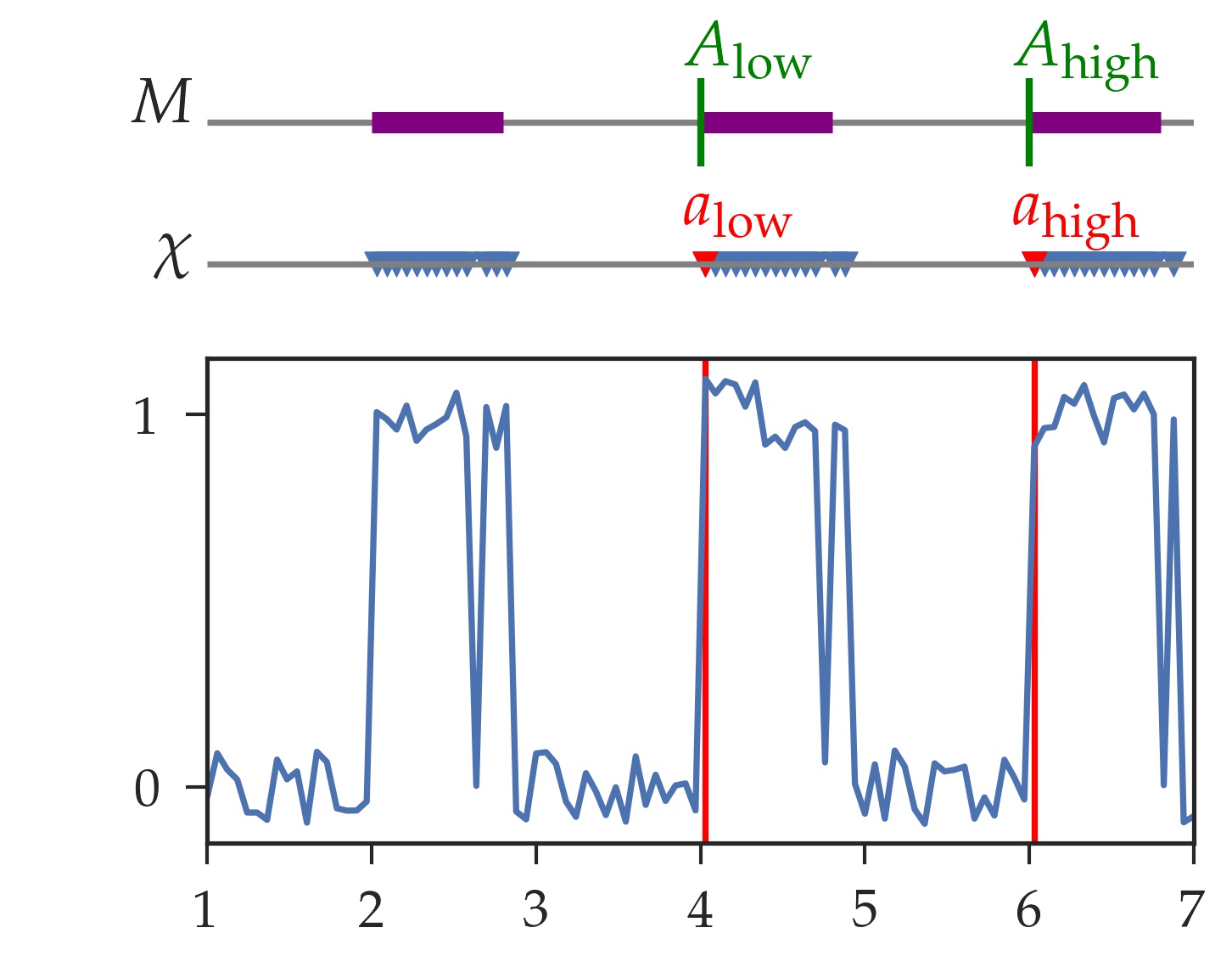
Counting the number of pulses in a range $[A,B]$ can be thought of as counting the number of connected components of $M=(P_{T}^{\tau})^{-1}(\{1\})\cap[A,B]$. With this in mind, we use a special case of 0-dimensional persistence to determine this from the point cloud approximation of $M$, namely $\chi=\{t_{i}\mid X(t_{i})>\tfrac{1}{2}\}$. See Figure 4 for an example.

In order to determine the persistence-based RPM $\Omega_{P}$, we need to find the range on the $t$-axis containing the full periods, and count the number of full periods there. In some sense, this procedure is measuring the voids between the components of $M$, rather than measuring the components of $M$ themselves. The following theorem essentially outlines an algorithm, which, given controlled enough noise, dense enough sampling, and enough visible pulses, calculates the number of pulses in that region using the persistence diagram $\mathrm{dgm}(\chi)$.

In particular, since $A_{\mathrm{low}}$ and $A_{\mathrm{high}}$ can be approximated within $\alpha\tau$ by

this theorem allows us to approximate the RPM in the following sections as

.

The pulse counting and RPM calculation can be obtained by transforming the signal to the frequency domain. Specifically, the one-sided Fourier transform of the signal is obtained after subtracting the mean value from it to remove the DC component from the spectrum. Then, the frequency $f$ in Hertz corresponding to the first amplitude $A$ that satisfies $A>A_{\text{max}}/w$ is found, where $w$ is a scalar, and the Fourier-based RPM $\Omega_{\text{F}}$ is calculated according to

In this study we chose $w=3$ since it provided accurate results for the studied cases with constant peak spacing. However, other values of $w$ did not improve the accuracy of the method for the cases with non-constant peak spacing, and therefore the deterioration in the performance of the Fourier-based approach for these case was not related to our choice of $w=3$.

We now create a generalized model for testing purposes where we have data which does not maintain regular pulses. This model will generate data on a window $[0,W]$. Assume $Q_{1},\cdots,Q_{K}$ are drawn iid from $\mathrm{unif}((1-\varepsilon)T,(1+\varepsilon)T)$. We assume $\varepsilon\in[0,1]$ and $K>\frac{W}{(1-\varepsilon)T}$ is large enough to ensure that $\sum_{i=1}^{K}Q_{i}\geq W$. We will generate pulses so that the length of the $i$th period is $Q_{i}$.

For the sake of notation, let $Q_{0}=0$. For any $s\in[0,W]$, define $\sigma(s)=\max\{j\in[0,\cdots,K]\mid\sum_{i=0}^{j}Q_{i}\leq s\}$. The reparameterization function is given by

Then the noisy time series is given as

where $\delta_{x}$ and $\delta_{y}$ are noise as defined in Sec. 3.1. See Fig. 3 for an example. Notice that this model simplifies to Eq. 1 when $\varepsilon=0$.

The left heat map in the bottom row of Fig. 5 shows that persistence performed significantly better than Fourier. Specifically, the relative error of the persistence algorithm is below $7\%$ for $\alpha<30\%$. In contrast, the error in Fourier is as high as $24\%$ for $\alpha<30\%$ and goes to at least $40\%$ for $\alpha>35\%$. Note that in both rows of Fig. 3 the color scale is the same. A closer look at the heat map of persistence in Fig. 6 shows how the error in the persistence algorithm is between $15\%$ and $25\%$ but only for $\alpha>30\%$. These are large values that correspond to a signal with very strong variations between the peaks. Note that even though we show the results for $\alpha\in[0,0.5]$, we could deal with the case of $\alpha>0.5$ by reversing the persistence algorithm from looking at the gaps between peaks (logic zero) to looking at logic one (high values in the two-level digital signal). Therefore, the user has the flexibility of adjusting the algorithm to recover good performance, as needed.

Figure 7 shows the plot of the average RPM versus $\alpha$ calculated using both persistence and Fourier for $\epsilon=25\%$ at three nominal rpms: $3178$ (top right), $12136$ (bottom left), and $20126$ (bottom right). The nominal RPM is indicated on the figure using a solid, horizontal black line. The curves for the calculated persistence and Fourier RPM values also include the $68\%$ confidence band that can be seen in the inset panels of the top right figure. These confidence bands were computed using an empirical bootstrap distribution of the sample mean. It can be seen that for $\alpha<20\%$, Fourier consistently underestimates all three nominal RPM values. Moreover, as $\alpha$ is increased beyond $20\%$, the Fourier estimate starts to decrease further below the nominal RPM. In contrast, persistence gives close estimates of the nominal RPM for $\alpha<25\%$, and only tends to consistently undershoot the nominal RPM for $\alpha>25\%$. Therefore, the bottom rows in Figs. 5 and 6 show that the persistence algorithm is robust to the width of the digital ringing.

The top row of Fig. 5 shows that for $\epsilon<7\%$ the two algorithms produce comparable results with less than $10\%$ relative error. However, as $\epsilon$ is increased, the performance of Fourier progressively deteriorates from $10\%$ to greater than $40\%$ as evidenced by the increase in the relative error across approximately four horizontal bands with a width of $10\%$ each. These bands are roughly given by $\epsilon\leq 15\%$, $18\%<\epsilon\leq 30\%$, $30\%<\epsilon\leq 40\%$, and $\epsilon>40\%$. In contrast, the left heat map in the first row shows that persistence consistently maintains less than $10\%$ error for almost all values of $\epsilon$; however, errors start to increase for $\epsilon>42\%$. The deterioration of the performance of the described approach is better observed from the heat map in Fig. 7 where higher relative errors start occurring towards the upper limit of the $\epsilon$ values.

In addition to the heat map that shows the relative error as a function of $\epsilon$ and $\Omega_{0}$, Fig. 7 shows the plot of the average RPM versus $\epsilon$ calculated using both persistence and Fourier for $\alpha=10\%$ at three nominal RPM values: $3178$ (top right), $12136$ (bottom left), and $20126$ (bottom right). The nominal RPM is indicated on the figure using a solid, horizontal black line. The curves for the calculated persistence and Fourier rpms also includes the $68\%$ confidence band that can be seen in the inset panels of the top right figure. These confidence bands were computed using an empirical bootstrap distribution of the sample mean. We can see that for both algorithms the confidence bands are narrow. Further, it can be seen that for $\epsilon<5\%$ both algorithms are close to the nominal value for all three RPM choices. However, for $\epsilon>5\%$, the Fourier algorithm quickly diverges away from the nominal RPM while persistence remains close to the nominal value. As $\epsilon$ is increased to $45\%$, we start to see persistence undershooting the nominal value which indicates that at high values of $\epsilon$, persistence undercounts the true peaks. Therefore, the top rows in Figs. 5 and 7 show that the persistence algorithm is robust to the variation in the spacing between the peaks.

In terms of theoretical runtime, the algorithm for computing $\Omega_{P}$ is simple, requiring only a sequence of pairwise subtractions and sortings. Since these take $O(n)$ and $O(n\log n)$ respectively, the theoretical worst case runtime for the persistence based algorithm is $O(n\log n)$. Meanwhile, the FFT algorithm computes the Fourier transform in $O(n\log n)$ as well, so the worst case analysis of the two methods is the same.

Runtime benchmarks for Fourier and persistence algorithms were measured using the performance counter from Python’s time package. The machine used for the simulations is a standard desktop running Ubuntu 16.04 with 32GB ram and a 3.6GHz Intel i7 processor. A total of $200$ runs for each algorithm was performed at each value of the nominal RPM. The nominal RPM is kept as a variable of runtime because it controls the length of the simulated pulse (see Table 1), and consequently, the runtime for each algorithm. The different runs were then averaged for each algorithm, and the results are plotted in Fig. 8. The line in the figure describes the average while the bands represent the $68\%$ confidence interval obtained by bootstrap sampling of the replicates. Notice the small $y$-axis scale in Fig. 8 indicating that both algorithms run relatively fast. However, the figure shows that persistence runs slightly faster than Fourier, and that the runtime is approximately constant across the RPM range. In contrast, the runtime for Fourier varies more than its persistence counterpart for the different values of the nominal RPM.

In essence, we have taken a difficult problem — clustering points in $\mathbb{R}^{d}$ — to a rather simplified setting — $d=1$. This restriction allows for very fast algorithms, particularly owing to the fact that one knows the minimal spanning tree in advance. Still, algorithms for computing 0-dimensional persistent homology for points in higher dimensions are still quite fast: an implementation using a modified union find algorithm runs in $O(n\alpha(n))$ where $n$ is the number of points and $\alpha$ is the notoriously slow growing inverse Ackermann function.

One could, however, imagine higher dimensional signals (i.e., images) where there are sufficient guarantees on the pulse rate and noise inputs so as to create higher dimensional analogues of Thm. 3.1. Consider, for example, the image of Fig. 11 generated by $Y(s,t)=X_{1}(s)\cdot X_{2}(t)$ for two realizations of Eqn. 1. The 0-dimensional persistence diagram histogram is shown to the right, and, as with the previous data shown in this paper, there is a clear distinction between the points. Since there are 35 points above a threshold of 8 in the histogram, we can conclude that there are 36 clusters in the image, which can be confirmed by inspection. Thus, we hypothesize that this method is quite useful in higher dimensional applications, although such an application is still an open question for future research.

References

- [1] Y. Sowa, A. D. Rowe, M. C. Leake, T. Yakushi, M. Homma, A. Ishijima, and R. M. Berry, “Direct observation of steps in rotation of the bacterial flagellar motor,” Nature, vol. 437, pp. 916–919, 2005.
- [2] M. A. Little and N. S. Jones, “Sparse Bayesian step-filtering for high-throughput analysis of molecular machine dynamics,” in 2010 IEEE International Conference on Acoustics, Speech and Signal Processing, pp. 4162–4165, March 2010.
- [3] M. A. Little and N. S. Jones, “Generalized methods and solvers for noise removal from piecewise constant signals. I. Background theory,” Proceedings of the Royal Society of London A: Mathematical, Physical and Engineering Sciences, vol. 467, no. 2135, pp. 3088–3114, 2011.
- [4] M. A. Little and N. S. Jones, “Generalized methods and solvers for noise removal from piecewise constant signals. II. New methods,” Proceedings of the Royal Society of London A: Mathematical, Physical and Engineering Sciences, vol. 467, no. 2135, pp. 3115–3140, 2011.
- [5] J. A. Nirody, Y.-R. Sun, and C.-J. Lo, “The biophysicist’s guide to the bacterial flagellar motor,” Advances in Physics: X, vol. 2, no. 2, pp. 324–343, 2017.
- [6] A. Youssef, D. Matthews, A. Guzzomi, and J. Pan, “Measurement of pressure fluctuations inside a model thrust bearing using PVDF sensors,” Sensors, vol. 17, no. 4, p. 878, 2017.
- [7] Y. Jin, S. Ji, B. Liu, and L. Chamorro, “On the role of thickness ratio and location of axis of rotation in the flat plate motions,” Journal of Fluids and Structures, vol. 64, pp. 127 – 137, 2016.
- [8] A. Albers, F. Schille, and M. Behrendt, “Method for measuring and analyzing transient powertrain vibrations of hybrid electric vehicles on an acoustic roller test bench,” in SAE Technical Paper, SAE International, 06 2016.
- [9] M. Rahman, T. Salyers, M. Ahmed, A. ElShahat, V. Soloiu, and E. Maroha, “Investigation of aerodynamic performance of helical shape vertical-axis wind turbine models with various number of blades using wind tunnel testing and computational fluid dynamics,” in ASME International Mechanical Engineering Congress and Exposition, vol. 7: Fluids Engineering, 2016.
- [10] G. Urbikain, D. Olvera, L. L. de Lacalle, and A. Elías-Zúñiga, “Spindle speed variation technique in turning operations: Modeling and real implementation,” Journal of Sound and Vibration, vol. 383, pp. 384 – 396, 2016.
- [11] S. Amini, M. Aghaei, M. Lotfi, and E. Hakimi, “Analysis of linear vibration in rotary turning of AISI 4140 steel,” International Journal of Advanced Manufacturing Technology, 2017.
- [12] B. Das, S. Bag, and S. Pal, “Defect detection in friction stir welding process through characterization of signals by fractal dimension,” Manufacturing Letters, vol. 7, pp. 6 – 10, 2016.
- [13] M. Wan, Y.-C. Ma, J. Feng, and W.-H. Zhang, “Mechanics of tapping process with emphasis on measurement of feed error and estimation of its induced indentation forces,” International Journal of Machine Tools and Manufacture, vol. 114, pp. 8 – 20, 2017.
- [14] A. Honeycutt and T. L. Schmitz, “Surface location error and surface roughness for period-n milling bifurcations,” Journal of Manufacturing Science and Engineering, vol. 139, pp. 061010 –061018, 2017.
- [15] R. Ghrist, Elementary Applied Topology. 2014.
- [16] H. Edelsbrunner and J. Harer, Computational Topology: An Introduction. American Mathematical Society, 2010.
- [17] T. Kaczynski, K. Mischaikow, and M. Mrozek, Computational Homology. Springer, 2004.
- [18] A. Zomorodian, Topology for Computing, vol. 16 of Cambridge Monographs on Applied and Computational Mathematics. Cambridge University Press, 2005.
- [19] R. Ghrist, “Barcodes: The persistent topology of data,” Builletin of the American Mathematical Society, vol. 45, pp. 61–75, 2008.
- [20] G. Carlsson, “Topology and data,” Bulletin of the American Mathematical Society, vol. 46, pp. 255–308, Jan. 2009.
- [21] V. Robins, J. D. Meiss, and E. Bradley, “Computing connectedness: An exercise in computational topology,” Nonlinearity, vol. 11, no. 4, p. 913, 1998.
- [22] V. Robins, J. Meiss, and E. Bradley, “Computing connectedness: disconnectedness and discreteness,” Physica D: Nonlinear Phenomena, vol. 139, no. 3, pp. 276 – 300, 2000.
- [23] V. Robins, N. Rooney, and E. Bradley, “Topology-based signal separation,” Chaos: An Interdisciplinary Journal of Nonlinear Science, vol. 14, no. 2, pp. 305–316, 2004.
- [24] M. Robinson, Topological Signal Processing. Springer, 2014.
- [25] Edelsbrunner, Letscher, and Zomorodian, “Topological persistence and simplification,” Discrete & Computational Geometry, vol. 28, no. 4, pp. 511–533, 2002.
- [26] A. Zomorodian and G. Carlsson, “Computing persistent homology,” Discrete & Computational Geometry, vol. 33, pp. 249–274, Nov. 2004.
- [27] J. Garland, E. Bradley, and J. D. Meiss, “Exploring the topology of dynamical reconstructions,” Physica D: Nonlinear Phenomena, vol. 334, pp. 49–59, nov 2016.
- [28] R. MacPherson and B. Schweinhart, “Measuring shape with topology,” Journal of Mathematical Physics, vol. 53, no. 7, 2012.
- [29] Z. Alexander, E. Bradley, J. D. Meiss, and N. F. Sanderson, “Simplicial multivalued maps and the witness complex for dynamical analysis of time series,” SIAM Journal on Applied Dynamical Systems, vol. 14, pp. 1278–1307, jan 2015.
- [30] S. Maletić, Y. Zhao, and M. Rajković, “Persistent topological features of dynamical systems,” Chaos: An Interdisciplinary Journal of Nonlinear Science, vol. 26, p. 053105, may 2016.
- [31] C. M. Pereira and R. F. de Mello, “Persistent homology for time series and spatial data clustering,” Expert Systems with Applications, no. 0, 2015.
- [32] J. A. Perea, “Persistent homology of toroidal sliding window embeddings,” in 2016 IEEE International Conference on Acoustics, Speech and Signal Processing (ICASSP), IEEE, mar 2016.
- [33] J. A. Perea and J. Harer, “Sliding windows and persistence: An application of topological methods to signal analysis,” Foundations of Computational Mathematics, pp. 1–40, 2015.
- [34] C. J. Tralie and J. A. Perea, “(Quasi)Periodicity quantification in video data, using topology,”
- [35] M. Robinson, “Universal factorizations of quasiperiodic functions,” in 2015 International Conference on Sampling Theory and Applications (SampTA), pp. 588–592, May 2015.
- [36] V. de Silva, P. Skraba, and M. Vejdemo-Johansson, “Topological analysis of recurrent systems,” in NIPS 2012 Workshop on Algebraic Topology and Machine Learning, 2012.
- [37] S. Emrani, T. Gentimis, and H. Krim, “Persistent homology of delay embeddings and its application to wheeze detection,” Signal Processing Letters, IEEE, vol. 21, pp. 459–463, April 2014.
- [38] Z. Alexander, J. D. Meiss, E. Bradley, and J. Garland, “Iterated function system models in data analysis: Detection and separation,” Chaos: An Interdisciplinary Journal of Nonlinear Science, vol. 22, no. 2, 2012.
- [39] M. Gidea and Y. Katz, “Topological data analysis of financial time series: Landscapes of crashes,” 2017.
- [40] M. Gidea, Topological Data Analysis of Critical Transitions in Financial Networks, pp. 47–59. Cham: Springer International Publishing, 2017.
- [41] M. Robinson, “Multipath-dominant, pulsed doppler analysis of rotating blades,” IET Radar Sonar and Navigation, vol. 7, pp. 217–224, Mar. 2013.
- [42] M. Vejdemo-Johansson, F. Pokorny, P. Skraba, and D. Kragic, “Cohomological learning of periodic motion,” Applicable Algebra in Engineering, Communication and Computing, pp. 1–22, 2015.
- [43] J. J. Berwald, M. Gidea, and M. Vejdemo-Johansson, “Automatic recognition and tagging of topologically different regimes in dynamical systems,” Discontinuity, Nonlinearity, and Complexity, vol. 3, no. 4, pp. 413–426, 2014.
- [44] F. A. Khasawneh and E. Munch, “Chatter detection in turning using persistent homology,” Mechanical Systems and Signal Processing, vol. 70-71, pp. 527–541, 2016.
- [45] F. A. Khasawneh and E. Munch, “Exploring equilibria in stochastic delay differential equations using persistent homology,” in Proceedings of the ASME 2014 International Design Engineering Technical Conferences & Computers and Information in Engineering Conference, August 17-20 , 2014, Buffalo, NY, USA, 2014. Paper no. DETC2014/VIB-35655.
- [46] F. A. Khasawneh and E. Munch, “Stability determination in turning using persistent homology and time series analysis,” in Proceedings of the ASME 2014 International Mechanical Engineering Congress & Exposition, November 14-20, 2014, Montreal, Canada, 2014. Paper no. IMECE2014-40221.
- [47] F. A. Khasawneh and E. Munch, Utilizing Topological Data Analysis for Studying Signals of Time-Delay Systems, pp. 93–106. Cham: Springer International Publishing, 2017.
- [48] A. Deckard, R. C. Anafi, J. B. Hogenesch, S. B. Haase, and J. Harer, “Design and analysis of large-scale biological rhythm studies: a comparison of algorithms for detecting periodic signals in biological data,” Bioinformatics, vol. 29, no. 24, pp. 3174–3180, 2013.
- [49] J. A. Perea, A. Deckard, S. B. Haase, and J. Harer, “SW1PerS: Sliding windows and 1-persistence scoring; discovering periodicity in gene expression time series data,” BMC Bioinformatics, vol. 16, Aug 2015.
- [50] D. Cohen-Steiner, H. Edelsbrunner, and J. Harer, “Stability of persistence diagrams,” Discrete Comput. Geom., vol. 37, pp. 103–120, Jan. 2007.
- [51] D. Cohen-Steiner, H. Edelsbrunner, J. Harer, and Y. Mileyko, “Lipschitz functions have -stable persistence,” Found. Comput. Math., vol. 10, pp. 127–139, Feb. 2010.
- [52] N. Otter, M. A. Porter, U. Tillmann, P. Grindrod, and H. A. Harrington, “A roadmap for the computation of persistent homology,” EPJ Data Science, vol. 6, aug 2017.
- [53] M. Stéphane, “Chapter 2 - the fourier kingdom,” in A Wavelet Tour of Signal Processing (Third Edition) (M. Stéphane, ed.), pp. 33 – 57, Boston: Academic Press, third edition ed., 2009.
- [54] A. Hatcher, Algebraic Topology. Cambridge University Press, 2002.
- [55] J. Munkres, Topology (2nd Edition). Pearson, 2000.
- [56] F. Murtagh and P. Contreras, “Algorithms for hierarchical clustering: an overview,” Wiley Interdisciplinary Reviews: Data Mining and Knowledge Discovery, vol. 2, pp. 86–97, dec 2011.
- [57] B. Sexton, J.S.and Stone, “The stability of machining with continuously varying spindle speed,” Annals of the CIRP, vol. 27, pp. 321–326, 1978.
- [58] A. Yilmaz, E. AL-Regib, and J. Ni, “Machine tool chatter suppression by multi-level random spindle speed variation,” Journal of Manufacturing Science and Engineering, vol. 124, no. 2, pp. 208–216, 2002.
- [59] S. Lin, R. DeVor, and S. Kapoor, “The effects of variable speed cutting on vibration control in face milling,” Journal of Engineering for Industry, vol. 112, pp. 1–11, 1990.
- [60] R. Radulescu, S. G. Kapoor, and R. E. DeVor, “An investigation of variable spindle speed face milling for tool-work structures with complex dynamics, part 1: Simulation results,” Journal of Manufacturing Science and Engineering, vol. 119, no. 3, pp. 266–272, 1997.