Regularization of Inverse Problems via
Time Discrete Geodesics in Image Spaces
Abstract
This paper addresses the solution of inverse problems in imaging given an additional reference image. We combine a modification of the discrete geodesic path model for image metamorphosis with a variational model, actually the - model, for image reconstruction. We prove that the space continuous model has a minimizer which depends in a stable way from the input data. Two minimization procedures which alternate over the involved sequences of deformations and images in different ways are proposed. The updates with respect to the image sequence exploit recent algorithms from convex analysis to minimize the - functional. For the numerical computation we apply a finite difference approach on staggered grids together with a multilevel strategy. We present proof-of-the-concept numerical results for sparse and limited angle computerized tomography as well as for superresolution demonstrating the power of the method.
1 Introduction
In certain applications it makes sense to account for qualitative prior image information to improve the image reconstruction. Typical examples are image superresolution and computerized tomography (CT) with sparsely or limited angle sampled sinogram data. Earlier approaches to incorporate prior knowledge on the image into CT include phase field methods [34, 47], the application of level set techniques, in particular when combining registration with segmentation [61], as well as the utilization of local (shape) descriptors [50, 69]. Recently, a mathematical classification of artifacts from arbitrary incomplete -ray tomography data using the classical filtered backprojection was given in [10]. For earlier papers on the this topic the reader may also consult [25, 26, 36, 48].
In this paper, we incorporate a whole reference image into the reconstruction process and take its deformation towards the image of interest, which is only indirectly given by measurements, into account. Recent work in this direction shows promising results. Schumacher, Modersitzki and Fischer [60] have dealt with the combined reconstruction and motion correction in SPECT imaging. Karlsson and Ringh [35] coupled the optimal transport model with inverse problems. Chen and Öktem [16] tackled hard inverse problems with shape priors under the name indirect image registration within the large deformation diffeomorphic metric mapping (LDDMM) framework and in an earlier paper [51] via linearized deformations. The authors use ODE constrained problem formulations, where the regularization of the deformations exploits reproducing kernel Hilbert spaces. As a drawback, the LDDMM [6, 17, 21, 62, 63] based methods can only deal with images having the same intensities. The metamorphosis model of Miller, Trouvé and Younes [42, 64, 65] is an extension of the LDDMM approach which allows the variation of the image intensities along trajectories of the pixels. A comprehensive overview over the topic is given in the book [70] as well as in the review article [41]. For a historic account see also [40]. In a recent preprint, Gris, Chen and Öktem [28] have enlarged the ideas in [16, 51] to the metamorphosis setting.
In our paper, we also follow the metamorphosis idea, but in a completely different way than in [28]. We built up on the time discrete geodesic calculus proposed for shape spaces by Rumpf and Wirth [57, 58] and for images by Berkels, Rumpf and Effland [7]. For convergence of the time discrete path model to the metamorphosis one we refer to these papers. Here deformations are modeled via a smoothness term and the linearized elastic potential, which is also a usual choice in registration problems. We combine this model with a ,,usual” variational image reconstruction model, actually the - model, which originated from [56]. Inspired by compressive sensing [13, 20] such variational image reconstruction techniques with sparsity-exploiting priors have achieved impressive reductions in sampling requirements. Besides TV priors, wavelet, shearlet- and curvelet representations [18, 24] were exploited in CT reconstructions with incomplete data.
Let be Hilbert spaces and a linear, continuous operator. A typical space will be the space of square integrable function defined over some image domain . We want to reconstruct an unknown image having the following information available:
- I1)
an image , where denotes some small error, e.g. due to noise.
- I2)
a reference image which is similar to the original image.
A usual variational model to approximate from using only I1) is given by
| (1) |
where is a data term and a prior or regularizer. A model for edge-preserving image reconstruction is the - model, which will be our model of choice.
To incorporate the reference image , we want to combine model (1) with a modified version of the time discrete geodesic model for image metamorphosis [7]. Given a template image and a reference image , this model aims to find a chain of smooth deformations from an appropriately defined admissible set together with a sequence of images such that the sum of the quadratic distances
| (2) |
together with a prior
on the deformations becomes small, see Fig. 1. The first part of the deformation regularization enforces the smoothness of the mappings, while the second term, circumscribed by , will be chosen as linearized elastic potential. By (2), the image sequence may differ from the deformed image sequence , which makes the model flexible for intensity changes.
For the numerical solution of our model we propose two different procedures, namely proximal alternating linearized minimization (PALM) [9] and an alternating minimization approach related to [7, 46]. For the later one, recent primal-dual minimization algorithms from convex analysis are merged with a Quasi-Newton approach from image registration.
Outline of the Paper
In Section 2, the necessary preliminaries concerning the spaces of deformations and images are introduced. In particular, we highlight properties of the concatenations of admissible deformations and images. This motivates the modification of the time discrete path model [7] and also of our generalized model for manifold-valued images in [46]. In Section 3, our space continuous reconstruction model is established. Since it combines time discrete morphing with inverse problems we call it TDM-INV. We prove that the functional has a minimizer and that the minimizer depends stably on the input data. Further, a convergence result for decreasing noise is provided. Section 4 deals with two minimization procedures. For minimizing the image sequence we incorporate primal-dual algorithms from convex analysis. Further, we explain computational issues in the space discrete setting. The numerical examples in Section 5 demonstrate the very good performance of our algorithm. We finish with conclusions in Section 6.
2 Preliminaries
In the rest of this paper, let be a nonempty, open, connected, and bounded set with Lipschitz boundary. In this section, we introduce admissible sets of deformations and consider the concatenation of deformations with images . Note that considered in [7] is in general not in while we will see that . Therefore, we prefer to modify the time discrete geodesic path model by using the later concatenation. Moreover, this fits better to the original metamorphosis setting of Tróuve and Younes. In [22] the image space is proposed instead and in [46] the computations are considerably simplified by using a set with deformations fulfilling for some fixed .
2.1 Admissible Deformations
First, we introduce the smoothness spaces of our deformation mappings. Let , , denote the Hölder space of functions for which
is finite. Equipped with this norm is a Banach space.
By , , , we denote the Sobolev space of functions having weak derivatives up to order in with norm
| (3) |
and semi-norm . For vector valued , the component wise norm is used. The space with is of particular interest, since it is compactly embedded in for all [1, Theorem 8.13] and consequently also for all .
It is assumed that the deformations are elements of the following admissible set
| (4) |
where . Then, by a result of Ball [3], has the following useful properties
- i)
.
- ii)
maps measurable sets in to measurable sets in and the change of variables formula
holds for any measurable set and any measurable function provided that one of the above integrals exists.
- iii)
is injective a.e., i.e., the set
has Lebesgue measure zero.
By property i) and since is bounded, it follows immediately for all that
| (5) |
with constants depending only on . By the embedding properties of Sobolev spaces it holds . Further, by the inverse mapping theorem, exists locally around a.e. and is continuously differentiable on the corresponding neighbourhood. However, to guarantee that is continuous (or, even more, continuously differentiable) on further assumptions are required, see [3, Theorem 2]. A possible counterexample is the function on , which is in but is not continuously differentiable.
2.2 Space of Images
In this paper, we consider images as functions in . Unfortunately, the concatenation of with can result in a function
as the example in and shows. However, this can be avoided by using
| (6) |
where the function needs to be defined properly. To this end, let be a Borel null set containing from iii). Then is a Borel set with . Note that is itself a Borel set since is measurable. Consider and let be a Borel set. Then, by ii), we see that is a Borel set, so that is a measurable function on . For and as above, the concatenation is measurable if defined as follows
| (7) |
Then, (6) can be verified by
which is finite since has components in . The same argument can be used to show that , if . Further, the following lemma on the image of null sets under the deformations and is useful.
Lemma 2.2.1.
For , both and its pre-image deformation map null sets to null sets.
Proof.
Since is Lipschitz continuous, it maps null sets to null sets [68, Theorem 3.33 and it’s proof]. Now assume that there exists a Borel null set with . Using the characteristic function on , we get the contradiction
∎
Finally, we prove a continuity result for the norm with respect to mappings .
Lemma 2.2.2.
Let , and be a sequence of deformations with for some . Then it holds
Proof.
Since , there exits a sequence of uniformly continuous functions with . Using the fact that maps null sets on null sets, we conclude
| (8) | ||||
| (9) | ||||
| (10) |
Due to the convergence of , there exists a constant such that for all . Thus,
| (11) | ||||
| (12) |
The last term converges to zero as . Now fix . Since converges uniformly to , the uniform continuity of can be used to conclude that converges uniformly to . Then boundedness of implies that the second term converges to zero as . For the first term the uniform continuity of implies that for every there exits large enough such that
| (13) | ||||
| (14) |
This concludes the proof. ∎
3 Space Continuous Model
In this section, we establish our space continuous model, which takes the information I1) and I2) into account and prove existence of minimizers, stability and convergence for vanishing noise. These three properties are necessary for a well-defined regularization method.
3.1 Model
Starting with the information I1), we are interested in reconstructing a two-dimensional image from its measurements based on the variational approach (1). In this paper, the main focus lies on the total variation semi-norm as regularizer . More precisely, recall that the space of functions of bounded variation consists of those functions having weak first order derivatives which are finite Radon measures. For , it holds that if and only if
The space becomes a Banach space with the norm . For , i.e. , the space can be continuously embedded into , see [2, Theorem 3.47]. Therefore, we can define
| (15) |
It is well-known that in (15) is a proper, convex and lower semi-continuous (lsc) functional on , see [59, Proposition 10.8].
Let be a continuous linear operator into a Hilbert space which does not vanish on constant functions and . In case of the Radon transform, it holds . Then, we define the variational reconstruction model
| (16) |
Note that is jointly weakly lsc in and .
Having a reference image available, we want to add information I2) to the model. To this end, let be a lsc mapping and , . Throughout the paper, it is assumed that is an integer. For a sequence of images in and a sequence of admissible deformations we consider the time discrete geodesic path model
| (17) |
where is a given reference image. Then, our whole model reads as
| (18) |
where . We call this model TDM-INV model referring to ’time discrete morphing - inverse’ problems.
Remark 3.1.1.
The linearized elastic potential is our choice for in (17). More precisely, rewriting the deformation as and introducing the notation of the (Cauchy) strain tensor of the displacement vector field as
we apply
| (19) |
Note that the linearized elastic potential is a usual regularizer in the context of registration, see [30, 43, 53].
3.2 Existence, Stability and Convergence
In this section, we prove that there exists a minimizer of in (18). Based on this, we show its stability with respect to the input data and the convergence of an image sequence obtained from minimizing the functionals with input data fulfilling for a zero sequence and corresponding parameters decaying faster than to .
The existence proof is the hardest part. As usual for functionals in two variables it is based on three pillars: First it is shown that a minimizer exists if one of the variables is fixed. In a second step the results are merged to get the overall existence.
Fixing the image sequence leads to the solution of single registration problems. The proof of Lemma 3.2.1 follows similar ideas as in [7, 46]. However, since the setting in those papers is different, we prefer to carefully follow the lines and make the necessary modifications to make the paper self-contained. Fixing , it is necessary to deal with the additional term and the proof of Lemma 3.2.2 is different from those in [7, 46], in particular it relies on nested weighted spaces. Except for the first step, the existence proof of Theorem 3.2.4 requires completely new estimates compared to [7, 46].
To begin with, we fix an image sequence and show that has a minimizer . Then, the consideration can be restricted to and it suffices to prove that each of the summands
| (20) |
for , has a minimizer in .
Lemma 3.2.1.
Let be a lsc mapping with the property
| (21) |
Further, let be given. Then there exists a minimizer of
| (22) |
over all .
Proof.
1. Let , , be a minimizing sequence
of .
Then it holds that for all .
This implies that has uniformly bounded semi-norm,
and by (5) the sequence is also uniformly bounded in
. Now we apply the Gagliardo-Nirenberg inequality, see Remark A.0.2, which states that for all it holds
| (23) |
All terms on the right-hand side are uniformly bounded. Hence, the norm of is uniformly bounded. Since is reflexive, there exists a subsequence which converges weakly to some function in . By the compact embedding , , this subsequence, which is again denoted by , converges strongly to in and hence converges uniformly to .
2. Next we show that is in the set . Since is lsc, we conclude
for all and since is nonnegative Fatou’s lemma implies
By incorporating (21) this implies a.e. Further, the boundary condition is fulfilled so that .
3. It remains to show that is a minimizer of . By Lemma 2.2.2, it holds as , so that by the continuity of the norm
This together with the previous steps of the proof implies that the three summands in are (weakly) lsc. Hence, we obtain
| (24) | ||||
| (25) |
which proves the claim. ∎
Next, we fix a sequence of mappings and ask for a minimizer of .
Lemma 3.2.2.
Let be a continuous linear operator into a Hilbert space which does not vanish on constant functions, and . For fixed , there exists a unique image sequence which minimizes .
Proof.
We prove lower semi-continuity, coercivity and strict convexity of the functional. Neglecting the constant terms and by changing the indexing of the sum it remains to consider
| (26) |
Setting
| (27) |
and substituting in the -th summand of (26), the functional transforms to
Using , where , , and , , we are concerned with the minimization of
| (28) | ||||
Note that by a.e. and , the weighted spaces are nested
| (29) |
in particular if . A minimizer must fulfill , and by successively considering the integrals in (28) further . In the following, we set to simplify the notation. Since the function ,
with and fixed, is strictly convex, the sum of the integrals in is strictly convex. Clearly, this sum can be rewritten as and is continuous. Since is proper, convex and lsc, the same holds true for over . Thus, is also weakly lsc [59, Lemma 10.4].
Next we show that is coercive. Assume conversely that but is bounded. By the assumptions on it holds that is coercive, see [11, Theorem 6.115]. Thus, is bounded and by (29) also is bounded. Considering successively the integrals in (28) we obtain that , is bounded which contradicts our assumption.
Thus, is coercive and since it is weakly lsc and strictly convex, the functional has a unique minimizer . By definition of the unique minimizer of is given by with . ∎
For our computations, the following corollary on the minimizer of in (28) with fixed will be useful.
Corollary 3.2.3.
Let be an integer. Further, let , fulfill a.e. on and , . For given and , the solution of
is given by
| (30) |
Proof.
Setting the first derivative of the functional to zero we obtain a.e. on ,
This can be rewritten as linear system of equations
Since the tridiagonal matrix is irreducible diagonal dominant, the system has a unique solution. Straightforward computation shows that the solution is given by (30). ∎
Now we can prove the three main results of this section, beginning with existence of minimizers.
Theorem 3.2.4 (Existence).
Let and . Then there exists minimizing .
Proof.
The outline of the proof is as follows. First, we take a minimizing sequence of and show that the deformations and the intermediate images have a weakly convergent subsequence. Then, we prove that their concatenation is also weakly convergent and use this to get the weak lower semi-continuity of the functional.
1. Let be a minimizing sequence of . Then for all . By Lemma 3.2.1, we find for each a sequence of diffeomorphisms such that
for all . Then, we know for all and . As in the first part of the proof of Lemma 3.2.1 we conclude that is bounded in , so that there exists a subsequence converging weakly in and strongly in to . Set and let us denote this subsequence again by and define .
2. Since for all , coercivity of implies that is bounded. Additionally, we conclude for that
Further, is convergent in and consequently on for . Then, it holds
Successive continuation shows that the sequence is bounded in . Hence, there exists a weakly convergent subsequence, also denoted by , which converges to .
3. Next, we show the weak convergence of to . Since the sequence is bounded, it suffices to test with . It holds
with
Using the change of variables formula, we obtain
Since , the weak convergence of to implies that converges to zero as . Using the change of variables formula again, can be estimated by
Since is bounded, it suffices to show the convergence of the second factor. With and it follows that
The first term converges to zero since is convergent. Uniform convergence of together with the uniform continuity of implies that converges uniformly to . Now boundedness of implies that the second term converges to zero.
4. It remains to show that is a minimizer of . It holds
The components of weakly converge in , those of converge in , and , weakly converges in . We use this together with the facts that the first summand is lsc, the second one weakly lsc and is weakly lsc (convex and lsc) in both arguments to conclude
Since is weakly lsc in we obtain
∎
Next, we prove that the minimizers of depend stably on the input data . To emphasize the dependence of on , we use the notation instead of .
Theorem 3.2.5 (Stability).
Let . Further, let be a sequence in converging to . For each , we choose a minimizer of . Then, there exists a subsequence of which converges weakly to a minimizer of .
Proof.
1. Due to the convergence of it holds for every that
Hence, there exists with for all . By definition of we obtain for all and . As in the first part of the proof of Lemma 3.2.1 we conclude that there exists a subsequence converging weakly in and strongly in to . Set . Let us denote this subsequence again by and define .
2. Next, we estimate
so that the coercivity of in implies the boundedness of . Now, we can reproduce the Steps 2 and 3 from Theorem 3.2.4 to see that there exists a weakly convergent subsequence, also denoted by , which converges to . Additionally, the sequence converges weakly to .
3. It remains to show that minimizes . We can use the lower semi continuity argument for from Theorem 3.2.4 together with the fact that is jointly lsc to obtain for any that
The last equality follows from the convergence of together with continuity of in . Hence, is a minimizer of . ∎
This section concludes with a convergence result for vanishing noise. Here we additionally need the dependence of on the parameter (for simplicity we choose ) and hence we use .
Theorem 3.2.6 (Convergence).
Let and , and suppose that there exists such that and . Further, assume that satisfies and as . Assume that is a sequence of positive numbers converging to 0 and is a sequence in satisfying for each . Let be a minimizer of , where . Then, there exists a subsequence of which weakly converges to an image such that .
Proof.
For every , it holds
From the assumptions on and we deduce that is bounded. Hence, there exists a weakly convergent subsequence with limit . Additionally, it holds . Now we can estimate
| (31) |
Since the two rightmost terms converge to zero, this implies . ∎
4 Minimization Approaches
In this section, we propose two different alternating minimization schemes. The first one is known as PALM and updates in each step the deformations and images via proximal computations. Convergence of the whole iteration sequence to a critical point is ensured. The second one just alternates the minimization of the deformations and the images.
Note that solving the coupled problem in e.g. with a gradient scheme is very time and memory consuming, since all and are treated at the same time. Moreover, the coupling is non-convex and hence it is difficult to provide convergence results for general schemes.
We start with the spatial discretization of in (18).
4.1 Spatial Discretization

Dealing with rectangular digital images, we propose a finite difference approach, where we work on staggered grids, see Fig. 2. In the following, the spatial discretization is briefly sketched. The domain of the images is the (primal) grid . All integrals are approximated on the integration domain by the midpoint quadrature rule, i.e., with pixel values defined on . Further, it is assumed that for the operator a discrete version is known, where is some finite dimensional Hilbert space.
First, we discuss the discretization of . As regularizer we propose the linearized elastic potential from Remark 3.1.1 with the replacement . Using the -shifted grids
we consider with and . Then, the spatially discrete version of reads
where is the Frobenius norm of matrices and denotes the forward differences operator (matrix) for in -direction. The higher order term with is discretized by
where central differences operators are used for the partial derivatives of order two and three. Note that we added the squared Frobenius norm of the , for a better control of the displacement value. To cope with the remaining deformation term in (17), we approximate such that the data term simplifies to
| (32) |
This integral is evaluated using the midpoint quadrature rule. Since is only defined on , and not on , the averaged version is used. In general , so that the image has to be interpolated from its values on . For this purpose linear interpolation with an interpolation matrix is used. Note that also interpolation matrices with higher space regularity or splines can be used. Summarizing, the discrete version of (17) reads
| (33) |
It remains to discretize , which is done by using the midpoint rule for the data term. For the TV-term the forward differences in , , direction are used
where the square and the square root are meant componentwise, and is the sum of the entries of the matrix. Then, the discrete functional reads
4.2 PALM
Our first approach for the minimization of is based on PALM [9, 55]. This algorithm aims to minimize a functional
| (34) |
by iterating
| (35) | ||||
| (36) |
where and denotes the proximal mapping of , which is uniquely determined for proper, convex and lsc functions . The convergence result is stated in the following theorem from [9, Theorem 1]. Note that in the theorem the proximal map is also defined for non-convex functions. However, the involved functions in our application are convex, so that no further details on this topic are provided.
Theorem 4.2.1.
Let be Euclidean spaces and , , , be proper, lsc functions. Assume that is continuously differentiable with locally Lipschitz continuous gradient and that both are globally Lipschitz, where the constants possibly depend on the fixed variable. Let in (34) fulfill the Kurdyka–Łojasiewicz (KL) property. Further, assume and for all . If the sequence generated by (35) is bounded, then it converges to a critical point.
For our problem we choose the splitting
| (37) | ||||
| (38) | ||||
| (39) |
Then the iteration (35) reads
| (40) | ||||
| (41) |
From the structure of we deduce that the , , can be computed separately. Note that the second term in can also be added to , but this only makes sense if is small since otherwise the Lipschitz constant gets too large. The , , can also be updated separately [9, Section 3.6], which possibly improves the Lipschitz constants. If the interpolation matrix originates from smooth piecewise polynomial basis functions and are chosen accordingly, all conditions of Theorem 4.2.1 are satisfied. The proximal map can be computed efficiently by primal-dual algorithms from convex analysis as for example by the Chambolle-Pock algorithm [14, 54]. Indeed there is a vast literature how to solve problems of this kind, see e.g. [12, 15] for an overview.
4.3 Alternating Minimization Approach
The computation of with a primal-dual algorithm requires an inner iteration for every step of PALM. If the evaluation of is computationally expensive, this can result in high computation effort due to many operator evaluations. Our numerical experiments indicated that PALM needs relatively many outer iterations and hence also many evaluations of the operator. Therefore, we want to present a second alternating scheme to minimize which needed fewer outer iterations in our experiments.
Starting with we iterate for :
1. For , we compute
| (42) |
2. For given , and , we solve
| (43) | ||||
For the first step the discretization from Section 4.1 is applied which results in the minimization of
| (44) |
for . This problem can be solved by a Quasi-Newton method, details can be found in [46, 53].
For the computation of the image sequence in the second step of the algorithm we use the substitution from the proof of Lemma 3.2.2. Setting , and , , we can transform (43) to
| (45) |
The functional is discretized on , using the approach from Section 4.1. We propose to solve the discrete version of (45) with a block-coordinate descent which fixes alternately and . For block-coordinate descent the following convergence result was proven in [4, Theorem 14.9, Theorem 14.15], see also [5].
Theorem 4.3.1.
Let be Euclidean spaces and , , be proper, convex lsc functions. Assume further that is continuously differentiable and that the level sets of are bounded. Then the minimization problem
can be solved by alternating minimization in and , i.e., every accumulation point of the generated iteration sequence is a minimizer. The convergence rate for the functional values is .
For our specific discretized problem (45) with
the conditions of the theorem are obviously fulfilled. If is fixed, Corollary 3.2.3 implies that the minimizer of is given analytically. In the second step of the algorithm we have to minimize, for fixed , the functional
| (46) |
This can be done efficiently by primal-dual algorithms from convex analysis, see Section 4.2 for a discussion. Finally, we use scattered interpolation to obtain the images at grid points from .
4.4 Multilevel Approach
As usual in optical flow and image registration, we apply a coarse-to-fine strategy with levels if a downsampling procedure for the data and the operator is known. This is the case for our numerical experiments, but it is also possible to use only a single level if no downsmapling procedure is known. First, we iteratively smooth our given template image by convolution with a truncated Gaussian and downsampling using bilinear interpolation. Here special care is necessary for the operator , as well as for the downsampling procedure of the data , which is dependent on the operator choice. Both procedures are described in the respective numerical examples.
In order to obtain a deformation on the coarsest level, a single registration is performed with the solution of the - problem, i.e.,
| (47) |
where is number of levels. For better results the regularization parameters for are decreased successively as recommended by Modersitzki [44].
After computing a solution on every level, bilinear interpolation is applied to construct an initial deformation on the next finer level. The sequence of , , intermediate finer level images is initialized from the end
| (48) |
where is the template image at the current level. Using this we obtain an initial image sequence on this level. The complete multilevel strategy is sketched in Algorithm 1 for the alternating minimization scheme presented in Section 4.3.
5 Numerical Examples
In this section, numerical examples demonstrating the potential of the method are presented. The proposed Algorithm 1 is implemented using Matlab. We also implemented the minimization of the TDM-INV model using PALM, but observed higher computation times due to many operator evaluations. For the Radon transform, the computation roughly needed two times as long (about 5-10 minutes). As comparison a result using PALM is added in the first example. The qualitative differences between the two results are very small and therefore only the results of Algorithm 1 are shown in the remaining experiments. Note that PALM might be more favourable if the operator is simple to evaluate, e.g. if it is sparse.
For representing our images on a grid during the registration step, we applied the mex interface of the spline library by E. Bertolazzi [8] with the Akima splines. In order to reduce the number of involved parameters in (44), we use in all our experiments. Typical choices for the increments are , and for the remaining levels. The remaining parameters , and are optimized with respect to the SSIM via a gridsearch. For the comparison algorithms the parameters are SIMM optimized, too. A GPU implementation is applied for solving the appearing linear systems of equations in the Quasi-Newton method.
In the first part of our experiments, the Radon transform is considered as operator. Among the vast literature on the topic, we refer to the books [32, 37, 45] for a general introduction to CT including some reconstruction methods from incomplete data and for limited angle tomography e.g. to [19, 33, 38]. The second part deals with superresolution, which does not have a continuous counterpart.
5.1 Limited Angle and Sparse CT
We are given a reference image and sinogram data of a target image , which we want to reconstruct. For the numerical implementation of the (discrete) Radon transform the Astra toolbox [52, 66, 67] is used, which allows more flexibility compared to the built-in Matlab function.
In our first example, the reference image consists of 6 triangular shaped objects, which are deformed to stars in the target image, see Fig. 311 1 The images in Fig. 3(a) and (b) are taken from the paper [16] and were provided by Barbara Gris and Ozan Öktem.. The sinogram is obtained by the Radon transform using 10 measurement directions equally distributed (with steps of 9 degrees) from 0 to 81 degrees, i.e. the measurement angle is limited to less than the half domain. The sinogram is additionally corrupted with 5 percent Gaussian noise. Our goal is to reconstruct the target from the given sinogram data. In the proposed multi grid approach a down-sampling by a factor of 0.5 is used. For the down-sampling of the sinogram, two neighboring rays are averaged and rescaled to the correct intensity. Note that this is easily possible if the number of rays is chosen for example to be 1.5 times the number of pixels per direction. The result of our TDM-INV algorithm is shown in Fig. 3 (c), where the parameters , , and are used. Compared to the reconstruction by the - model (with ) in Fig. 3 (f), our method is able to better deal with the missing data from 81 to 180 degrees. Visually, the result is almost perfect and also the SSIM value is very good. In Fig. 3 (d) the numerical result using PALM is shown. The SSIM and PSNR values are similar to Fig. 3 (c) and almost no difference is visible. The difference of both results is depicted in Fig. 3 (e) and lies within the color range .


(SSIM .9815, PSNR 30.31)

(SSIM .9815, PSNR 30.40)
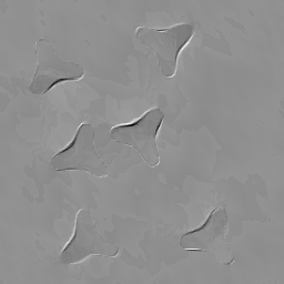

(SSIM .9377, PSNR 24.89)
In the second example a more structured image is treated. The given reference image depicts an artificial brain image, and the target can be considered as a deformed version, see Fig. 422 2 Available at http://bigwww.epfl.ch/algorithms/mriphantom/, see also [29].. The sinogram of the target is created using the Radon transform with 20 measurements equally distributed from 0 to 180 degrees and by adding 5 percent Gaussian noise.


(SSIM .7542, PSNR 26.47)

(SSIM .6819, PSNR 24.20)
For the multi grid approach the procedure from the previous example is used. The result of TDM-INV is shown in Fig. 4 (c) and was calculated with the parameters , , and . Since our model incorporates the reference information as compensation for the sparse data set, the reconstruction is better than the one with the - model (with ) in Fig. 4 (d).
5.2 Superresolution


(SSIM .8111, PSNR 25.76)

(SSIM .8075, PSNR 24.75)
Here, we are given a reference image and a low resolution image obtained by down-sampling of a target image with the down-sampling operator given by
In other words, . For the multi grid approach a downscaling with factor is applied such that the given image can be used for the first three levels, i.e., . The matrix is adapted to for the second level and the identity matrix of corresponding size is used for all higher levels.
In our third example the same reference and target images as in the second example are used, see Fig. 5. The result of TDM-INV is shown in Fig. 5 (d), where the parameters , , and are used. First, our method is compared with the single image superresolution method of He and Siu [31], which is based on a self-similarity assumption of the high and low resolution image together with a Gaussian process regression. In contrast to the result obtained by this method in Fig. 5 (e), our result does not have artifacts around the bright features. Using the Matlab function imresize, the best reconstruction is obtained with the “lanczos3” kernel, see Fig. 5 (f), which is affected by a strong blur. For this example, the - (parameter ) reconstruction yields the result shown in Fig. 5 (g). Comparing all methods, we see that our method is best at recovering the fine details as well as the overall structure.


(SSIM .8474, PSNR 26.38)

(SSIM .9226, PSNR 27.49)
In our last example , the template image is not only deformed and scaled, but also a new detail is included in the image. As mass can be created on the image path, our method is able to reconstruct also the small detail, cf. Fig. 6 33 3 The images used in Fig. 6 are based on the ones in [28]., where the parameters are chosen as , , and . For this simpler image, our method leads to the best result in SSIM and PSNR. The result produced by [31] in Fig. 6 (e) yields almost the same SSIM , but visually the method recovers a lot of background noise. The best result of Matlab’s imresize is given by the “bilinear” interpolation here. However, this result is affected by a strong blur. The - approach (parameter ) works better for this simpler image than in the previous example, but is still not able to match our result. Especially the overlapping part in the center of the phantom is only recovered by TDM-INV.
6 Conclusions
This paper merges the edge-preserving - variational model for solving inverse image reconstruction problems with a metamorphosis-inspired approach to utilize information from a reference image. The approach, called TDM-INV, can handle intensity changes between the reference image and the target image which we want to reconstruct. The method gives very good results for artificial images so that we are looking forward to real-world applications in material sciences or medical imaging, e.g. motion models for organs [23, 27]. Several extensions of the model are possible. Due to the finite difference approach and the design of the method more sophisticated regularizers than the TV-term can be simply involved. Another possible modification would be to apply different transport models, see e.g. [39]. Further, the usage of multiple reference images can be taken into account.
Appendix A Gagliardo-Nirenberg Inequality
Theorem A.0.1 (Gagliardo-Nirenberg [49]).
Let be a bounded domain satisfying the cone property. For , suppose that belongs to and its derivatives of order to . Then for the derivatives , , the following inequalities hold true with constants independent of :
where for all , except for the case and is a nonnegative integer, in which the inequality only holds true for .
Remark A.0.2.
For the inequality simplifies to
where the second inequality follows by estimating the product with the maximum of both factors.
Acknowledgments
This work was initialized during an internship of S. Neumayer in the research group of C. Schönlieb at the University of Cambridge. S. Neumayer wants to thank B. Gris, O. Öktem and C. Schönlieb for stimulating talks on the topic. Further, we want to thank A. Effland for discussions on PALM. Funding by the German Research Foundation (DFG) within the project STE 571/13-1 and within the Research Training Group 1932, project area P3, is gratefully acknowledged. We gratefully acknowledge the support of NVIDIA Corporation with the donation of the Quadro M5000 GPU used for this research.
References
- [1] H. W. Alt. Lineare Funktionalanalysis: Eine anwendungsorientierte Einführung, volume 6. Springer, Berlin, 2002.
- [2] L. Ambrosio, N. Fusco, and D. Pallara. Functions of Bounded Variation and Free Discontinuity Problems. Oxford University Press, 2000.
- [3] J. M. Ball. Global invertibility of Sobolev functions and the interpenetration of matter. Proceedings of the Royal Society of Edinburgh: Section A Mathematics, 88(3-4):315–328, 1981.
- [4] A. Beck. First-Order Methods in Optimization, volume 25. SIAM, 2017.
- [5] A. Beck and L. Tetruashvili. On the convergence of block coordinate descent type methods. SIAM Journal on Optimization, 23(4):2037–2060, 2013.
- [6] M. F. Beg, M. I. Miller, A. Trouvé, and L. Younes. Computing large deformation metric mappings via geodesic flows of diffeomorphisms. International Journal of Computer Vision, 61(2):139–157, 2005.
- [7] B. Berkels, A. Effland, and M. Rumpf. Time discrete geodesic paths in the space of images. SIAM Journal on Imaging Sciences, 8(3):1457–1488, 2015.
- [8] E. Bertolazzi. Splines toolbox. https://github.com/ebertolazzi/Splines.
- [9] J. Bolte, S. Sabach, and M. Teboulle. Proximal alternating linearized minimization for nonconvex and nonsmooth problems. Mathematical Programming, 146(1-2, Ser. A):459–494, 2014.
- [10] L. Borg, J. Frikel, J. Sauer-Jorgensen, and E. T. Quinto. Full characterization of reconstruction artifacts from arbitrary incomplete X-ray CT data. ArXiv Preprint, 1701.03055v3, 2018.
- [11] K. Bredies and D. Lorenz. Mathematische Bildverarbeitung. Vieweg+Teuber, 2011.
- [12] M. Burger, A. Sawatzky, and G. Steidl. First order algorithms in variational image processing. In S. O. R. Glowinski and W. Yin, editors, Operator Splittings and Alternating Direction Methods, Springer 2017, 2017.
- [13] E. J. Candés, J. Romberg, and T. Tao. Stable signal recovery from incomplete and inaccurate measurements. Communications in Pure and Applied Mathematics, 59:1207––1223, 2006.
- [14] A. Chambolle and T. Pock. A first-order primal-dual algorithm for convex problems with applications to imaging. Journal of Mathematical Imaging and Vision, 40(1):120–145, 2011.
- [15] A. Chambolle and T. Pock. An introduction to continuous optimization for imaging. Acta Numerica, 25:161–319, 2016.
- [16] C. Chen and O. Öktem. Indirect image registration with large diffeomorphic deformations. SIAM Journal on Imaging Sciences, 11(1):575–617, 2018.
- [17] G. E. Christensen, R. D. Rabbitt, and M. I. Miller. Deformable templates using large deformation kinematics. IEEE Transactions on Image Processing, 5(10):1435–1447, 1996.
- [18] F. Colonna, G. Easley, K. Guo, and D. Labate. Radon transform inversion using the shearlet representation. Applied and Computational Harmonic Analysis, 29(2):232––250, 2010.
- [19] M. E. Davison. The ill-conditioned nature of the limited angle tomography problem. SIAM Journal on Applied Mathematics, 43(2):428––448, 1983.
- [20] D. Donoho. Compressed sensing. IEEE Transactions on Information Theory, 52:1289–1306, 2006.
- [21] P. Dupuis, U. Grenander, and M. I. Miller. Variational problems on flows of diffeomorphisms for image matching. Quarterly of Applied Mathematics, 56(3):587–600, 1998.
- [22] A. Effland. Discrete Riemannian Calculus and A Posteriori Error Control on Shape Spaces. Dissertation, University of Bonn, 2017.
- [23] J. Ehrhardt and C. Lorenz. 4D Modeling and Estimation of Respiratory Motion for Radiation Therapy. Springer, 2013.
- [24] J. Frikel. Sparse regularization in limited angle tomography. Applied and Computational Harmonic Analysis, 34:117––141, 2013.
- [25] J. Frikel and E. T. Quinto. Characterization and reduction of artifacts in limited angle tomography. Inverse Problems, 29(12):125007, 2013.
- [26] J. Frikel and E. T. Quinto. Limited data problems for the generalized radon transform in . SIAM Journal on Mathematical Analysis, 48(4):2301–2318, 2016.
- [27] F. Gigengack, X. Jiang, M. Dawood, and K. P. Schäfers. Motion Correction in Thoracic Positron Emission Tomography. Springer, 2015.
- [28] B. Gris, C. Chen, and O. Öktem. Image reconstruction through metamorphosis. HAL Preprint hal-01773633v1, Apr. 2018.
- [29] M. Guerquin-Kern, L. Lejeune, K. P. Pruessmann, and M. Unser. Realistic analytical phantoms for parallel magnetic resonance imaging. IEEE Transactions on Medical Imaging, 31(3):626–636, 2012.
- [30] E. Haber and J. Modersitzki. A multilevel method for image registration. SIAM Journal on Scientific Computing, 27(5):1594–1607, 2006.
- [31] H. He and W.-C. Siu. Single image super-resolution using Gaussian process regression. In 2011 IEEE Conference on Computer Vision and Pattern Recognition (CVPR), pages 449–456. IEEE, 2011.
- [32] G. T. Herman. Image Reconstructions from Projections. The Fundamentals of Computerized Tomography. Academic Press, 1980.
- [33] G. T. Herman and R. Davidi. Image reconstruction from a small number of projections. Inverse Problems, 24(4):045011, 2008.
- [34] R. J. Hewett, I. Jermyn, M. Heath, and F. Kamalabadi. A phase field method for tomographic reconstruction from limited data. In Proceedings of the British Machine Vision Conference, pages 1–11. BMVA Press, 2012.
- [35] J. Karlsson and A. Ringh. Generalized Sinkhorn iterations for regularizing inverse problems using optimal mass transport. SIAM Journal on Imaging Sciences, 10(4):1935–1962, 2017.
- [36] A. I. Katsevich. Local tomography for the limited-angle problem. Journal of Mathematical Analysis and its Applications, 213:160–182, 1997.
- [37] P. Kuchment. The Radon Transform and Medical Imaging. SIAM, Philadelphia, 2014.
- [38] A. K. Louis. Incomplete data problems in X-ray computerized tomography. Numerische Mathematik, 48(3):251–262, 1986.
- [39] J. Maas, M. Rumpf, C. Schönlieb, and S. Simon. A generalized model for optimal transport of images including dissipation and density modulation. ESAIM: Mathematical Modelling and Numerical Analysis, 49(6):1745–1769, 2015.
- [40] M. I. Miller, A. Trouvé, and L. Younes. On the metrics and Euler-Lagrange equations of computational anatomy. Annual Review of Biomedical Engineering, 4(1):375–405, 2002.
- [41] M. I. Miller, A. Trouvé, and L. Younes. Hamiltonian systems and optimal control in computational anatomy: 100 years since d’arcy thompson. Annual Review of Biomedical Engineering, 17:447–509, 2015.
- [42] M. I. Miller and L. Younes. Group actions, homeomorphisms, and matching: A general framework. International Journal of Computer Vision, 41(1-2):61–84, 2001.
- [43] J. Modersitzki. Numerical Methods for Image Registration. Oxford University Press on Demand, 2004.
- [44] J. Modersitzki. FAIR: Flexible Algorithms for Image Registration. SIAM, Philadelphia, 2009.
- [45] F. Natterer. The Mathematics of Computerized Tomography. Classics in Applied Mathematics. SIAM, Philadelphia, 2001.
- [46] S. Neumayer, J. Persch, and G. Steidl. Morphing of manifold-valued images inspired by discrete geodesics in image spaces. SIAM Journal on Imaging Sciences, 11(3):1898–1930, 2018.
- [47] L. H. Nguyen, S. K. F. Stoter, T. Baum, J. S. Kirschke, M. Ruess, Z. Yosibash, and D. Schillinger1. Phase-field boundary conditions for the voxel finite cell method: surface-free stress analysis of ct-based bone structures. International Journal for Numerical Methods in Biomedical Engineering, 33(12):1–34, 2017.
- [48] L. V. Nguyen. How strong are streak artifacs in limited angle computed tomography? Inverse Problems, 31:055003, 2015.
- [49] L. Nirenberg. An extended interpolation inequality. Annali Della Scuola Normale Superiore di Pisa-Classe di Scienze, 20(4):733–737, 1966.
- [50] M. A. Nogueira, P. H. Abreu1, P. Martins, P. Machado1, H. Duarte, and J. Santos. Image descriptors in radiology images: a systematic review. Artificial Intelligence Review, 47:531––559, 2017.
- [51] O. Öktem, C. Chen, N. O. Domaniç, P. Ravikumar, and C. Bajaj. Shape-based image reconstruction using linearized deformations. Inverse Problems, 33(3):035004, 2017.
- [52] W. Palenstijn, K. Batenburg, and J. Sijbers. Performance improvements for iterative electron tomography reconstruction using graphics processing units (gpus). Journal of Structural Biology, 176(2):250–253, 2011.
- [53] J. Persch, F. Pierre, and G. Steidl. Exemplar-based face colorization using image morphing. Journal of Imaging, 3(4):Art.Num. 48, 2017.
- [54] T. Pock, A. Chambolle, D. Cremers, and H. Bischof. A convex relaxation approach for computing minimal partitions. IEEE Conference on Computer Vision and Pattern Recognition, pages 810–817, 2009.
- [55] T. Pock and S. Sabach. Inertial proximal alternating linearized minimization (iPALM) for nonconvex and nonsmooth problems. SIAM J. Imaging Sci., 9(4):1756–1787, 2016.
- [56] L. Rudin, S. Osher, and E. Fatemi. Nonlinear total variation based noise removal algorithms. Physica D, 60:259–268, 1992.
- [57] M. Rumpf and B. Wirth. Discrete geodesic calculus in shape space and applications in the space of viscous fluidic objects. SIAM Journal on Imaging Sciences, 6(4):2581–2602, 2013.
- [58] M. Rumpf and B. Wirth. Variational time discretization of geodesic calculus. IMA Journal of Numerical Analysis, 35(3):1011–1046, 2015.
- [59] O. Scherzer, M. Grasmair, H. Grossauer, M. Haltmeier, and F. Lenzen. Variational Methods in Imaging. Springer, 2009.
- [60] H. Schumacher, J. Modersitzki, and B. Fischer. Combined reconstruction and motion correction in spect imaging. IEEE Transactions on Nuclear Science, 56(1):73–80, 2009.
- [61] P. Swierczynski, B. W. Papiez, J. A. Schnabel, and C. Macdonald. A level-set approach to joint image segmentation and registration with application to ct lung imaging. Computerized Medical Imaging and Graphics, 65:58–68, 2018.
- [62] A. Trouvé. An infinite dimensional group approach for physics based models in pattern recognition. International Journal of Computer Vision, 1995.
- [63] A. Trouvé. Diffeomorphisms groups and pattern matching in image analysis. International Journal of Computer Vision, 28(3):213–221, 1998.
- [64] A. Trouvé and L. Younes. Local geometry of deformable templates. SIAM Journal of Mathematical Analysis, 37(2):17–59, 2005.
- [65] A. Trouvé and L. Younes. Metamorphoses through Lie group action. Foundations in Computational Mathematics, 5(2):173–198, 2005.
- [66] W. van Aarle, W. J. Palenstijn, J. Cant, E. Janssens, F. Bleichrodt, A. Dabravolski, J. De Beenhouwer, K. J. Batenburg, and J. Sijbers. Fast and flexible X-ray tomography using the ASTRA toolbox. Optics Express, 24(22):25129–25147, 2016.
- [67] W. van Aarle, W. J. Palenstijn, J. De Beenhouwer, T. Altantzis, S. Bals, K. J. Batenburg, and J. Sijbers. The ASTRA toolbox: A platform for advanced algorithm development in electron tomography. Ultramicroscopy, 157:35–47, 2015.
- [68] R. L. Wheeden. Measure and Integral: an Introduction to Real Analysis, volume 308. CRC Press, 2015.
- [69] W. Yang, L. Zhong, L. Lin, Y. Chen, Z. Lu, S. Liu, Y. Wu, Q. Feng, and W. Chen. Predicting ct image from mri data through feature matching with learned nonlinear local descriptors. IEEE Transactions on Medical Imaging, in print.
- [70] L. Younes. Shapes and Diffeomorphisms. Springer-Verlag, Berlin, 2010.