In Topological Data Analysis one studies high dimensional data sets by extracting shapes. Many of these shapes are $2$-dimensional simplicial complexes where it is computationally possible to calculate topological invariants such as homology groups (see for example [12]). $2$-complexes that are amenable for more detailed analysis are $2$-dimensional stratified spaces, which occur in the study of persistent homology of high-dimensional data [2], [3]. Special classes of these stratified spaces are foams, which occur as special spines of 3-dimensional manifolds [13], [14]. Khovanov [11] used trivalent foams to construct a bigraded homology theory whose Euler characteristic is a quantum $sl(3)$ link invariant and Carter [4] presented an analogue of the Reidemeister-type moves for knotted foams in $4$-space. One would like to obtain a classification of 2-dimensional stratified spaces in terms of algebraic invariants, but this class is too large, even when restricted to foams. However, there is a smaller class of $2$-dimensional stratified spaces, namely those with empty $0$-stratum, called $2$-stratifolds, for which such a classification is feasible. A closed $2$-stratifold is a $2$-dimensional cell complex $X$ that contains a collection of finitely many simple closed curves, the components of the $1$-skeleton $X^{(1)}$ of $X$, such that $X-X^{(1)}$ is a $2$-manifold and a neighborhood of each component $C$ of $X^{(1)}$ consists of $n\geq 3$ sheets (a precise definition is given in section 2). In particular, if the number of sheets is three, then $X$ is called trivalent. Such $2$-stratifolds also arise in the study of categorical invariants of $3$-manifolds. For example if $\mathcal{G}$ is a non-empty family of groups that is closed under subgroups, one would like to determine which (closed) $3$-manifolds have $\mathcal{G}$-category equal to $3$. In [5] it is shown that such manifolds have a decomposition into three compact $3$-submanifolds $H_{1},H_{2},H_{3}$ , where the intersection of $H_{i}\cap H_{j}$ (for $i\neq j$) is a compact $2$-manifold, and each $H_{i}$ is $\mathcal{G}$-contractible (i.e. the image of the fundamental group of each connected component of $H_{i}$ in the fundamental group of the $3$-manifold is in the family $\mathcal{G}$). The nerve of this decomposition, which is the union of all the intersections $H_{i}\cap H_{j}$ ($i\neq j$), is a closed $2$-stratifold and determines whether the $\mathcal{G}$-category of the 3-manifold is $2$ or $3$.

When trying to classify $2$-stratifolds one first looks at their fundamental groups. Free groups, surface groups, Baumslag-Solitar groups (Hopfian or non-Hopfian), $F$-groups are realized as fundamental groups of $2$-stratifolds. The question of which (closed) $3$-manifold groups are $2$-stratifold groups was solved in [10]. Very few $3$-manifolds have $2$-stratifold spines. Since $3$-manifold groups have solvable word problem ([1]), the question arises whether this is true for $2$-stratifold groups. An affirmative answer was proved in [9].

A $2$-stratifold is essentially determined by its associated bipartite labelled graph (defined in section 2) and a presentation for its fundamental group can be read off from the labelled graph. Thus the question arises when a labelled graph determines a simply connected $2$-stratifold. In [7] an algorithm on the labelled graph was developed for determining whether the graph determines a simply connected $2$-stratifold and in [8] we obtained a complete classification of all trivalent labelled graphs that represent simply connected $2$-stratifolds.

In the present paper we develop three operations on labelled graphs that will construct from a single vertex all trivalent graphs that represent simply connected $2$-stratifolds. In section 6 an implementation of these three operations and some results from [8] is described. It was coded using Python and NetworkX.

We first review the basic definitions and some results given in [6] and [7]. A $2$-stratifold is a compact, Hausdorff space $X$ that contains a closed (possibly disconnected) $1$-manifold $X^{(1)}$ as a closed subspace with the following property: Each point $x\in X^{(1)}$ has a neighborhood homeomorphic to $\mathbb{R}{\times}CL$, where $CL$ is the open cone on $L$ for some (finite) set $L$ of cardinality $>2$ and $X-X^{(1)}$ is a (possibly disconnected) $2$-manifold.

A component $B\approx S^{1}$ of $X^{(1)}$ has a regular neighborhood $N(B)=N_{\pi}(B)$ that is homeomorphic to $(Y{\times}[0,1])/(y,1)\sim(h(y),0)$, where $Y$ is the closed cone on the discrete space $\{1,2,...,d\}$ and $h:Y\to Y$ is a homeomorphism whose restriction to $\{1,2,...,d\}$ is the permutation $\pi:\{1,2,...,d\}\to\{1,2,...,d\}$. The space $N_{\pi}(B)$ depends only on the conjugacy class of $\pi\in S_{d}$ and therefore is determined by a partition of $d$. A component of $\partial N_{\pi}(B)$ corresponds then to a summand of the partition determined by $\pi$. Here the neighborhoods $N(B)$ are chosen sufficiently small so that for disjoint components $B$ and $B^{\prime}$ of $X^{(1)}$, $N(B)$ is disjoint from $N(B^{\prime})$. The components of $\overline{N(B)-B}$ are called the sheets of $N(B)$.

For a given $2$- stratifold $(X,X^{(1)})$ there is an associated bipartite graph $\Gamma=\Gamma(X,X^{(1)})$ embedded in $X$ as follows:

In each component $B_{j}$ of $X^{(1)}$ choose a black vertex $b_{j}$. In the interior of each component $W_{i}$ of $M=\overline{X-\cup_{j}N(B_{j})}$ choose a white vertex $w_{i}$. In each component $C_{ij}$ of $W_{i}\cap N(B_{j})$ choose a point $y_{ij}$, an arc $\alpha_{ij}$ in $W_{i}$ from $w_{i}$ to $y_{ij}$ and an arc $\beta_{ij}$ from $y_{ij}$ to $b_{j}$ in the sheet of $N(B_{j})$ containing $y_{ij}$. An edge $e_{ij}$ between $w_{i}$ and $b_{j}$ consists of the arc $\alpha_{ij}*\beta_{ij}$. For a fixed $i$, the arcs $\alpha_{ij}$ are chosen to meet only at $w_{i}$.

We label the graph $\Gamma$ by assigning to a white vertex $W$ its genus $g$ of $W$ and by labelling an edge $C$ by $r$, where $r$ is the summand of the partition $\pi$ corresponding to the component $C$ of $\partial N_{\pi}(B)$ where $C\subset\partial N_{\pi}(B)$. (Here we use Neumann’s [15] convention of assinging negative genus $g$ to nonorientable surfaces). White vertices of genus $0$ are not labelled. Note that the partition $\pi$ of a black vertex is determined by the labels of the adjacent edges. If $\Gamma$ is a tree, then the labeled graph determines $X$ uniquely.

Another description of $X_{\Gamma}$ is as a quotient space $W\cup_{\psi}X^{(1)}$, where $W=\bigcup W_{i}$ and where $\psi:\partial W\to X^{(1)}$ is a covering map (and $|\psi^{-1}(x)|>2$ for every $x\in X^{(1)}$). For a component $C=S^{1}$ of $\partial W$ the label $r$ on the corresponding edge then corresponds to the attaching map $\psi(z)=z^{r}$.

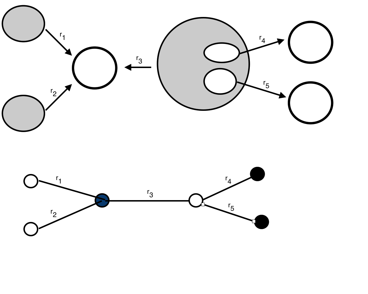
The following two propositions are shown in [6].

(Here $c_{1},\dots,c_{p}$ correspond to the boundary curves of the $p$-times

punctured $S^{2}$ that corresponds to $w$).

For example for the graph of Figure 1 we read off the following presentation of $\pi_{1}(X_{\Gamma})=\{b_{1},b_{2},b_{3},c_{1},c_{2},c_{3},c_{4},c_{5}\,|\,c_{1}=1,c_{2}=1,c_{3}c_{4}c_{5}=1,\,b_{1}^{r_{1}}=c_{1},b_{2}^{r_{2}}=c_{2},b_{3}^{r_{3}}=c_{3},b_{3}^{r_{4}}=c_{4},b_{3}^{r_{5}}=c_{5}\}=\{b_{1},b_{2},b_{3}\,|\,\,b_{1}^{r_{1}}=1,b_{2}^{r_{2}}=1,b_{3}^{r_{3}+r_{4}+r_{5}}=1\}$.

On a labeled graph $\Gamma=\Gamma_{X}$ with all white vertices of genus $0$ consider the following operation $O1$ that changes $\Gamma=\Gamma_{X}$ to $\Gamma_{1}=\Gamma_{X_{1}}$:

If $b_{i}$ is the black vertex incident to the edge labeled $r_{i}$ then the corresponding relation $b_{1}^{r_{1}}\dots b_{m}^{r_{m}}=1$ in $\pi_{1}(X)$ is changed to the relations $b_{1}^{r_{1}}\dots b_{k}^{r_{k}}b=1$, $b=1$, $b_{k+1}^{r_{k+1}}\dots b_{m}^{r_{m}}=1$ in $\pi_{1}(X_{1})$ and it follows that $\pi_{1}(X_{1})$ is a quotient of $\pi_{1}(X)$. In particular we note:

The building blocks for constructing labeled trivalent graphs for 1-connected $2$-stratifolds are called $b12$-trees and $b111$-trees:

For two disjoint labeled graphs $\Gamma_{1}=\Gamma_{X_{1}}$ and $\Gamma_{2}=\Gamma_{X_{2}}$ with all white vertices of genus $0$, operation $O1*$ described in Figure 5, creates a new graph $\Gamma=\Gamma_{X}$:

Note that $X$ is obtained from $X_{1}$ and $X_{2}$ by identifying a disk in $X_{1}$ with a disk in $X_{2}$, therefore :

Finally, on a labeled graph $\Gamma=\Gamma_{X}$ with all white vertices of genus $0$ consider operation $O2$ described in Figure 4, that changes $\Gamma=\Gamma_{X}$ to $\Gamma_{1}=\Gamma_{X_{1}}$:

We now describe the collection $\mathcal{G}$ of all trivalent graphs that can be obtained from a single white vertex by successively applying Operations $O1$ and $O2$.

For a collection $\mathcal{C}$ of bipartite labeled graphs denote by $\widehat{\mathcal{C}}$ the collection of all compact, connected bipartite labeled graphs obtained by starting with any $\Gamma_{0}\in\mathcal{C}$ and successively performing Operations $O1$ or $O2$. We express this as

$\widehat{\mathcal{C}}=\{\emptyset,\Gamma_{0}\stackrel{{\scriptstyle O^{1}}}{{\longrightarrow}}\dots\stackrel{{\scriptstyle O^{m}}}{{\longrightarrow}}\Gamma\,\,|\,\,\Gamma_{0}\in\mathcal{C},\,O^{i}=O1\text{ or }O2\,;\,m\geq 0\,\}$

Let $\circ$ denote (the collection containing only) the graph consisting of one white vertex and let $\mathcal{G}_{0}=\widehat{\circ}$ .

For two connected bipartite labeled graphs $\Gamma$ and $\Gamma^{\prime}$ denote by $\Gamma\bot\Gamma^{\prime}$ a graph obtained by joining any white vertex of $\Gamma$ to any white vertex of $\Gamma^{\prime}$ by operation $O1^{*}$. Note that that there are $nn^{\prime}$ such $\Gamma\bot\Gamma^{\prime}$, where $n$ (resp. $n^{\prime}$) is the number of white vertices of $\Gamma$ (resp. $\Gamma^{\prime}$). Let

$\mathcal{G}_{0}\bot\mathcal{G}_{0}=\{\,\Gamma\bot\Gamma^{\prime}\,|\,\Gamma,\Gamma^{\prime}\in\mathcal{G}_{0}\,\}$

In particular, $\mathcal{G}_{0}\bot\emptyset=\mathcal{G}_{0}$ and $\emptyset\bot\emptyset=\emptyset$. Let

$\mathcal{G}_{1}=\widehat{\mathcal{G}_{0}\bot\mathcal{G}_{0}}$, and inductively $\mathcal{G}_{n+1}=\widehat{\mathcal{G}_{n}\bot\mathcal{G}_{n}}$

Then $\mathcal{G}_{0}\subset\mathcal{G}_{1}\subset\dots\subset\mathcal{G}_{n}\subset\dots\,\,\subset\mathcal{G}:=\bigcup_{i=0}^{\infty}\mathcal{G}_{i}$

In the next section an implementation of the constructions in the two previous sections is given. The motivation for some of the examples comes from the following classification theorem in [8].

For convenience we here recall the definitions of the terms used in this theorem.

$B$ denotes the union of all the black vertices of degree $3$ of $G$ and $st(B)$ is the (open) star of $B$ in $G$.

A $(2,1)$-collapsible tree is a bi-colored tree constructed as follows:
Start with a rooted tree $T$ (which may consist of only one vertex) with root $r$ (a vertex of $T$), color with white and label $0$ the vertices of $T$, take the barycentric subdivision $sd(T)$ of $T$, color with black the new vertices (the barycenters of the edges of $T$) and finally label an edge $e$ of $sd(T)$ with $2$ (resp. $1$) if the distance from $e$ to the root $r$ is even (resp. odd). (We allow a one-vertex tree (with white vertex) as a $(2,1)$- collapsible tree).

The reduced subgraph $R(G)$ is defined for a bi-colored labeled tree $G$ for which the components of $G-st(B)$ are $(2,1)$-collapsible trees. It is the graph obtained from $St(B)$ (the closed star of $B$) by attaching to each white vertex $w$ of $St(B)$ that is not a root, a $b12$-graph such that the terminal edge has label $2$.

Finally, A horned tree is a bi-colored tree constructed as follows:
Start with a tree $T$ that has at least two edges and all of whose nonterminal vertices have degree $3$. Color a vertex of $T$ white (resp. black) if it has degree $1$ (resp. $3$). Trisect the terminal edges of $T$ and bisect the nonterminal edges, obtaining the graph $H_{T}$. Color the additional vertices $v$ so that $H_{T}$ is bipartite, that is, $v$ is colored black if $v$ is a neighbor of a terminal vertex of $H_{T}$ and white otherwise. Then label the edges such that every terminal edge has label $2$, every nonterminal edge has label $1$.

An implementation for some parts of this paper and [8], mainly the algorithm for checking if a labelled graph determines a simply connected 2-stratifold, was coded using Python (v3.6.4) and the module NetworkX (v2.1) [16]. A link for downloading the code from a github repository is included. Coded examples and a file with details on the implementation can also be found in that repository.

By construction, a graph of a $2$-stratifold is bipartite, but it is possible for it to have more than one edge between a black and a white vertex. As all edges are undirected, the class strat_graph is implemented as a subclass of MultiGraph (which is part of the NetworkX module).

The color of each node is stored as an 0-1 attribute, namely ’bipartite’, which is equal to 0 for white vertices and 1 for black ones. The labels for the edges were stored as an integer attribute called ’weight’. Up to this point we are only interested in graphs which have all white vertices with label 0, so this attribute for white nodes is not yet implemented.

The module (strat.py), along with a readme file and examples (examples.py), may be downloaded from https://github.com/yair-hdz/stratifolds.

Troughout the code, the word node is also used to refer to vertices. The following methods belong to the class strat_graph:

• •

  __init__(self,black=[],white=[],edges=None): the initializer of this class.

• •

  addEdg(self,edges): a function for adding edges.

• •

  addNod(self, black=[], white=[]): a funcion for adding black or white vertices.

• •

  black_vals(self): returns a dictionary where the keys are the black vertices and values are the sum of the labels of the edges incident to that node (which, in the case of a trivalent stratifold, must equal 3).

• •

  is_trivalent(self): returns True if the graph is trivalent, False otherwise.

• •

  white(self): returns a set object with the white vertices. black(self) does the same for black vertices.

• •

  copy(self): returns a copy of the strat_graph instance.

• •

  is_horned_tree(self): returns True if the graph is a horned tree (definition 3.3 from [8]), and False otherwise.

• •

  is_21_collapsible(self): if self is a 2,1-collapsible tree (defined before lemma 3.2 in [8]), returns the root of the tree. Otherwise, returns None.

• •

  subg(self,nodes): returns a subgraph from self with nodes as set of nodes, where an edge occurs if and only both vertices belong to nodes. All labels are preserved.

• •

  St_B(self): returns a list of the connected components of $St(B)$ (notation from [8]: $St(B)$ is the closed star of $B$, the set of vertices with degree 3), where each component is a strat_graph instance.

• •

  graph_stB(self): returns a list of the components of $G\setminus st(B)$, where (using notation from [8]) $st(B)$ is the open star of $B$.

• •

  is_simply_connected(self): implementation of theorem 3.6 from [8]. Returns True if self is the graph of a simply connected trivalent $2$-stratifold.

• •

  O1(self,white_node,black_nodes1,black_nodes2,W0=None,W1=None, B=None): returns a copy of self where operation $O1$ has been performed on the vertex white_node.

• •

  O1_1(self,node,other,node_other, black=None,white=None): performs operation $O1*$ if self and other are disjoint graphs.

• •

  O2(self,white_node,new_white=None,new_black=None): performs operation $O2$ on vertex white_node.

• •

  draw(self,trivalent=False): Function for drawing a graph. Calls the function draw from networkx, coloring black vertices black and white vertices gray. If trivalent=True, asserts if graph is trivalent and then draws the graph with edges with label 2 bold.

Additionaly, the module has functions b111 and b12 for generating $b111$- and $b12$-trees.

For further details on each method, refer to the readme file from the repository.

References

- [1] M. Aschenbrenner, S. Friedl, H. Wilton, -manifold groups, European Math.Soc. (2015).
- [2] P. Bendich, B. Wang, S. Mukherjee, Towards Stratification Learning through Homology Inference, arXiv:1008.3572v1 [math.GT] (2010).
- [3] P. Bendich, E. Gasparovic, C. J. Tralie, J. Harer, Scaffoldings and Spines: Organizing High-Dimensional Data Using Cover Trees, Local Principal Component Analysis, and Persistent Homology, arXiv:1602.06245v2 (2016).
- [4] J.S. Carter, Reidemeister/Roseman-type moves to embedded foams in 4-dimensional space, in “New Ideas in Low Dimensional Topology”, Series on Knots and Everything Volume 56, 1-30 (2015).
- [5] J.C. Gómez-Larrañaga, F. González-Acuña, Wolfgang Heil, Categorical group invariants of 3-manifolds, manuscripta math. 145, 433-448 (2014).
- [6] J.C. Gómez-Larrañaga, F. González-Acuña, Wolfgang Heil, -stratifolds, in “A Mathematical Tribute to José María Montesinos Amilibia”, Universidad Complutense de Madrid, 395-405 (2016).
- [7] J.C. Gómez-Larrañaga, F. González-Acuña, Wolfgang Heil, -dimensional stratifolds homotopy equivalent to , Topology Appl. 209, 56-62 (2016).
- [8] J.C. Gómez-Larrañaga, F. González-Acuña, Wolfgang Heil, Classification of Simply-connected Trivalent -dimensional Stratifolds, Top. Proc. (2018)
- [9] J.C. Gómez-Larrañaga, F. González-Acuña, Wolfgang Heil, -stratifold groups have solvable Word Problem, Revista de la Real Academia de Ciencias Exactas, Físicas y Naturales. Serie A. Matemáticas, Online First Articles ISSN: 1578-7303 (Print) 1579-1505 (Online)
- [10] J.C. Gómez-Larrañaga, F. González-Acuña, Wolfgang Heil, -stratifold spines of closed -manifolds, arXiv:1707.05663 (2017).
- [11] M. Khovanov, sl(3) link homology. Algebr. and Geom. Topol. 4, 1045-1081 (2004).
- [12] P. Lum, G. Singh, J. Carlsson, A. Lehman, T. Ishkhanov, M. Vejdemo-Johansson, M. Alagappan, G. Carlsson, Extracting insights from the shape of complex data using topology. Nature Scientific Reports 3, 12-36 (2013).
- [13] S.V. Matveev, Distributive groupoids in knot theory; (Russian) Mat. Sb. (N.S.) 119(161) (1982), no. 1, 78-88, 160.
- [14] R. Piergallini, Standard moves for standard polyhedra and spines, Third National Conference on Topology (Italian) (Trieste, 1986). Rend. Circ. Mat. Palermo (2) Suppl. No. 18 (1988), 391-414.
- [15] W. Neumann, A calculus for plumbing applied to the topology of complex surface singularities and degenerating complex curves, Trans. Amer. Math. Soc. 268, 299-344 (1981).
- [16] A. Hagberg, Daniel A. Schult and Pieter J. Swart, “Exploring network structure, dynamics, and function using NetworkX”, in Proceedings of the 7th Python in Science Conference (SciPy2008), Gäel Varoquaux, Travis Vaught, and Jarrod Millman (Eds), (Pasadena, CA USA), pp. 11–15, Aug 2008.