跳到论文正文
W Papers独立论文阅读器 arXiv:1805.06185 论文正文 计算阅读时间 · 0%
引用这篇论文根据当前论文元数据生成,正式投稿前建议核对。


License: arXiv.org perpetual non-exclusive license
arXiv:1805.06185v3 [math.NA] 05 Nov 2018

Locality estimates for Fresnel-wave-propagation and stability of X-ray phase contrast imaging with finite detectorsThanks: Submitted to the editors of Inverse Problems on May 16, 2018.

Simon Maretzke ††thanks: Institute for Numerical and Applied Mathematics, University of Goettingen, Lotzestrasse 16-18, 37083 Göttingen, Germany (). Email: simon.maretzke@googlemail.com
Abstract

Coherent wave-propagation in the near-field Fresnel-regime is the underlying contrast-mechanism to (propagation-based) X-ray phase contrast imaging (XPCI), an emerging lensless technique that enables 2D- and 3D-imaging of biological soft tissues and other light-element samples down to nanometer-resolutions. Mathematically, propagation is described by the Fresnel-propagator, a convolution with an arbitrarily non-local kernel. As real-world detectors may only capture a finite field-of-view, this non-locality implies that the recorded diffraction-patterns are necessarily incomplete. This raises the question of stability of image-reconstruction from the truncated data – even if the complex-valued wave-field, and not just its modulus, could be measured. Contrary to the latter restriction of the acquisition, known as the phase-problem, the finite-detector-problem has not received much attention in literature. The present work therefore analyzes locality of Fresnel-propagation in order to establish stability of XPCI with finite detectors. Image-reconstruction is shown to be severely ill-posed in this setting – even without a phase-problem. However, quantitative estimates of the leaked wave-field reveal that Lipschitz-stability holds down to a sharp resolution limit that depends on the detector-size and varies within the field-of-view. The smallest resolvable lengthscale is found to be ≈1/¯​𝔣\approx\!1/\lower 3.87495pt\hbox{$\mathchar 22$}\mkern-8.0mu\mathfrak{f} times the detector’s aspect length, where ¯​𝔣\lower 3.87495pt\hbox{$\mathchar 22$}\mkern-8.0mu\mathfrak{f} is the Fresnel number associated with the latter scale. The stability results are extended to phaseless imaging in the linear contrast-transfer-function regime.

keywords
Fresnel propagation, image reconstruction, stability, resolution, X-ray imaging, phase contrast
Funding.
This work was funded by Deutsche Forschungsgemeinschaft DFG through Project C02 of SFB 755 - Nanoscale Photonic Imaging.
††runningheads: Locality estimates for Fresnel-wave-propagation / Simon Maretzke
AMS
65R32, 92C55, 94A08 78A45, 78A46

1 Introduction

State-of-the-art high-resolution imaging techniques are a driving force behind current biomedical- and material science. Among such, (propagation-based) X-ray phase contrast imaging (XPCI), also known as near-field holography, stands out as it yields two- or three-dimensional images down to nanometer-resolutions with high penetration-depths at relatively low radiation-dose and sample-preparation requirements [34, 26, 24, 7, 2, 19, 13, 9].

Refer to caption
Figure 1: Exemplary experimental setup for (propagation-based) X-ray phase contrast imaging (XPCI) at synchrotrons (sketch of the GINIX-experiment [28] at P10-beamline, DESY).

The setup of XPCI is appealingly simple, see the example sketched in fig. 1: essentially, it boils down to a coherent X-ray beam illuminating an unknown object and a detector that records the resulting near-field diffraction pattern, also termed hologram, at a finite distance behind the sample. The coherent wave-propagation from the sample to the detector, described by the Helmholtz equation in the paraxial- of Fresnel-approximation [11, 22], is essential as it enables phase-contrast: it partially encodes phase-shifts in the complex-valued X-ray wave-field Ψ\Psi induced by refraction within the sample into measurable wave intensities ∝|Ψ|2\propto|\Psi|^{2}, thereby circumventing the well-known phase problem, i.e. the inability to measure the phase of Ψ\Psi directly. This permits imaging of biological soft tissues and other light-element samples, for which the absorption of X-rays – but not refraction – is negligible [26].

To obtain an interpretable image of the sample, the induced phase-shifts (and absorption) have to be reconstructed from the measured hologram(s), i.e. an inverse problem has to be solved. By the limitation of the data to the squared modulus |Ψ|2|\Psi|^{2}, this requires to recover the missing phase-information. For the present setting, however, this task is comparably well-understood by now and routinely solved using data from multiple sample-detector-distances along with a linearization of the contrast known as the contrast-transfer-function (CTF) model [7, 31, 14, 13] and/or additional a priori knowledge on the recovered images [3, 2, 25, 19]. Indeed, it is shown in previous work that the mild assumption of a known compact support of the image ensures well-posedness of the reconstruction in the linear CTF-regime [20].

What is typically tacitly ignored, however, is the data-incompleteness arising from the finiteness of the field-of-view captured by the detector due to the de-localizing action of (Fresnel-)wave-propagation: existing theory mostly assumes data within the complete infinite detector-plane and most reconstruction methods implicitly assume periodic detector-boundaries, possibly combined with artificial extension of the data by padding. While this produces reasonable results in practice, theoretical understanding for the effects of a finite detector and of the associated heuristic corrections is lacking.

This work aims to close this gap of theory by deriving rigorous estimates on the locality of information-transport by wave-propagation in the Fresnel-regime with the ultimate goal of extending existing stability estimates for XPCI to settings with finite detectors. In particular, the focus is on the question of resolution:

  • Given an XPCI setup, what is the size of the smallest sample-features that can be stably reconstructed from the measured data?

In physics literature [21, 15], authors typically refer to Abbe’s diffraction limit [5, 17], defining the resolution via the numerical aperture associated with the detector-size. However, the underlying reasoning is heuristic and motivated by far-field optics, despite the near-field setting of the imaging technique. Rigorous theory is thus necessary to supplement physical intuition.

The manuscript is organized as follows: §\lx@sectionsign2 introduces the mathematical setting and notation as well as some preliminary insights on the finite-detector problem. In §\lx@sectionsign3, the relation between resolution and detector-size is assessed by the study of Gaussian wave-packets, yielding best-case estimates in some sense. These are then complemented by worst-case estimates on stability of image-reconstruction derived in §\lx@sectionsign4, §\lx@sectionsign5 and §\lx@sectionsign6 under different a priori assumptions on the unknown objects. Having derived all of these results under the simplifying assumption that also the phase of the data is measured, the obtained locality- and stability estimates are then extended to the phaseless case of linearized XPCI in §\lx@sectionsign7. §\lx@sectionsign8 concludes this work.

Despite the focus on XPCI, note that the derived estimates may be extended to a wide range of wave-propagation problems from classical physics and quantum-mechanics.

2 Background

2.1 Basic setting

2.1.1 Fresnel-propagation

We consider the problem of reconstructing a function h:ℝm→ℂh:\mathbb{R}^{m}\to\mathbb{C} from partial knowledge of Fresnel-data:

𝒟⁡(h)\displaystyle\mathcal{D}(h) :=ℱ(m𝔣⋅ℱ−1(h))withm𝔣(𝝃):=exp(−i𝝃2/(2𝔣)),𝔣>0,𝝃∈ℝm.\displaystyle:=\mathcal{F}\left(m_{\mathfrak{f}}\cdot\mathcal{F}^{-1}(h)\right)\;\;\;\;\;\text{with}\;\;\;\;\;m_{\mathfrak{f}}(\boldsymbol{\xi}):=\exp\left(-{\text{{i}}\boldsymbol{\xi}^{2}}/{(2\mathfrak{f})}\right),\quad\mathfrak{f}>0,\,\boldsymbol{\xi}\in\mathbb{R}^{m}. (2.1)

ℱ(f)(𝝃):=(2π)−m/2∫ℝmexp(−i𝝃⋅𝒙)f(𝒙)d𝒙\mathcal{F}(f)(\boldsymbol{\xi}):=(2\pi)^{-m/2}\int_{\mathbb{R}^{m}}\exp(-\text{{i}}\boldsymbol{\xi}\cdot\boldsymbol{x})f(\boldsymbol{x})\,\text{{d}}\boldsymbol{x} denotes the mm-dimensional Fourier transform. The Fresnel-propagator 𝒟\mathcal{D} models the free-space propagation of time-harmonic wave-fields Ψ⁡(𝒙,z)=Ψ~​(𝒙,z)​exp⁡(i​𝔣​z)\Psi(\boldsymbol{x},z)=\tilde{\Psi}(\boldsymbol{x},z)\exp(\text{{i}}\mathfrak{f}z) with slowly varying envelope Ψ~\tilde{\Psi} within the regime of the paraxial Helmholtz-equation (see e.g. [22] for details):

{(2i𝔣∂z+Δ𝒙)Ψ~(𝒙,z)=0(𝒙,z)∈ℝm×(0;1)Ψ~​(𝒙,0)=h​(𝒙)𝒙∈ℝm⇒Ψ~​(⋅,1)=𝒟⁡(Ψ~​(⋅,0))\displaystyle\begin{cases}\left(2\text{{i}}\mathfrak{f}\partial_{z}+\Delta_{\boldsymbol{x}}\right)\tilde{\Psi}(\boldsymbol{x},z)=0&(\boldsymbol{x},z)\in\mathbb{R}^{m}\times(0;1)\\ \tilde{\Psi}(\boldsymbol{x},0)=h(\boldsymbol{x})&\boldsymbol{x}\in\mathbb{R}^{m}\end{cases}\quad\Rightarrow\quad\tilde{\Psi}(\cdot,1)=\mathcal{D}\left(\tilde{\Psi}(\cdot,0)\right) (2.2)
Refer to caption
Figure 2: Schematic model of propagation-based XPCI: incident plane waves are scattered by a sample, imprinting phase-shifts and absorption h=−i​ϕ−μh=-\text{{i}}\phi-\mu upon the transmitted wave-field Ψ⁡(⋅,0)\Psi(\cdot,0) within the object-domain Ω\Omega. The intensity of the resulting near-field diffraction pattern I=|Ψ⁡(⋅,d)|2I=|\Psi(\cdot,d)|^{2} is recorded within the detection-domain KK at some distance behind the object.

2.1.2 Forward models

As detailed in [26, 11, 22, 20], Fresnel-diffraction data arises in X-ray phase contrast imaging (XPCI): if the incident beam in fig. 1 is modeled by a plane wave as sketched in fig. 2, the wave-field in the object’s exit-plane z=0z=0 is

Ψ~​(⋅,0)\displaystyle\tilde{\Psi}(\cdot,0) =exp(h)withh=−iϕ−μ=−ik∫ℝ(δ−iβ)dz,\displaystyle=\exp(h)\;\;\;\;\;\text{with}\;\;\;\;\;h=-\text{{i}}\phi-\mu=-\text{{i}}k\int_{\mathbb{R}}\big(\delta-\text{{i}}\beta\big)\text{{d}}z, (2.3)

(within some standard approximations of X-ray optics [11]), where n⁡(𝒙,z)=1−δ⁡(𝒙,z)+i​β​(𝒙,z)n(\boldsymbol{x},z)=1-\delta(\boldsymbol{x},z)+\text{{i}}\beta(\boldsymbol{x},z) is the spatially varying refractive index of the sample. The complex-valued image hh is thus a projection of the sample-characterizing quantities δ,β\delta,\beta. As the wave-field in the detector-plane relates to Ψ~​(⋅,0)\tilde{\Psi}(\cdot,0) via Fresnel-propagation, the detected intensities are given by

I⁡(𝒙)=|𝒟⁡(Ψ~​(⋅,0))​(𝒙)|2=|𝒟⁡(exp⁡(h))​(𝒙)|2.\displaystyle I(\boldsymbol{x})=\big|\mathcal{D}\big(\tilde{\Psi}(\cdot,0)\big)(\boldsymbol{x})\big|^{2}=\left|\mathcal{D}\big(\exp(h)\big)(\boldsymbol{x})\right|^{2}. (2.4)

Under the additional assumption that the object is sufficiently weakly scattering for the image to be “small” in a suitable sense, (2.4) may be linearized:

I=1+𝒯⁡(h)+𝒪⁡(h2)with𝒯⁡(h)=2​Re​(𝒟⁡(h)),\displaystyle I=1+\mathcal{T}(h)+\mathcal{O}(h^{2})\;\;\;\;\;\text{with}\;\;\;\;\;\mathcal{T}(h)=2\textup{Re}(\mathcal{D}(h)), (2.5)

where Re is the pointwise real part. In Fourier-space, the contrast in the phase-shifts ϕ\phi and attenuation μ\mu is then described by oscillatory contrast-transfer-functions (CTF):

ℱ⁡(𝒯⁡(−i​ϕ−μ))​(𝝃)=−2​sin⁡(|𝝃|2/(2​𝔣))​ℱ​(ϕ)​(𝝃)−2​cos⁡(|𝝃|2/(2​𝔣))​ℱ​(μ)​(𝝃)\displaystyle\mathcal{F}\big(\mathcal{T}(-\text{{i}}\phi-\mu)\big)(\boldsymbol{\xi})=-2\sin\left(|\boldsymbol{\xi}|^{2}/(2\mathfrak{f})\right)\mathcal{F}(\phi)(\boldsymbol{\xi})-2\cos\left(|\boldsymbol{\xi}|^{2}/(2\mathfrak{f})\right)\mathcal{F}(\mu)(\boldsymbol{\xi}) (2.6)

for all 𝝃∈ℝm\boldsymbol{\xi}\in\mathbb{R}^{m}. Therefore, the linearized XPCI-model is also termed CTF-model.

Furthermore, it is often assumed [23, 31] that the object is homogeneous, in the sense that refraction and absorption are proportional: h=−μ−i​ϕ=−ie−i​α​φh=-\mu-\text{{i}}\phi=-\text{{i}}\text{{e}}^{-\text{{i}}\alpha}\varphi for some α∈[0;π)\alpha\in[0;\pi) and a real-valued function φ\varphi. In the linearized case, this yields a modified CTF-model:

𝒮α​(φ):=𝒯⁡(h)=−2​ℱ−1​(sα⋅ℱ⁡(φ)),sα​(𝝃):=sin⁡(|𝝃|2/(2​𝔣)+α)\displaystyle\mathcal{S}_{\alpha}(\varphi):=\mathcal{T}(h)=-2\mathcal{F}^{-1}\left(s_{\alpha}\cdot\mathcal{F}(\varphi)\right),\quad s_{\alpha}(\boldsymbol{\xi}):=\sin\left(|\boldsymbol{\xi}|^{2}/(2\mathfrak{f})+\alpha\right) (2.7)

The case α=0\alpha=0 corresponds to pure phase objects which induce negligible absorption μ≈0\mu\approx 0.

2.1.3 Object- and detection-domains

We assume that the approximate size of the imaged object is known a priori. Then there exists a bounded object-domain Ω⊂ℝm\Omega\subset\mathbb{R}^{m} such that the unknown image hh satisfies supp(h)={𝒙∈ℝm:h⁡(𝒙)≠0}¯⊂Ω\supp(h)={}\mkern 3.0mu\overline{\mkern-3.0mu\{\boldsymbol{x}\in\mathbb{R}^{m}:h(\boldsymbol{x})\neq 0\}}\subset\Omega, where the overbar denotes set-closure. We consider the L2L^{2}-functions satisfying this support-constraint:

h∈L2(Ω):={h:ℝm→ℂ:supp(h)⊂Ω,∫ℝm|h|2d𝒙<∞}.\displaystyle h\in L^{2}(\Omega):=\big\{h:\mathbb{R}^{m}\to\mathbb{C}:\supp(h)\subset\Omega,\,{\textstyle\int_{\mathbb{R}^{m}}|h|^{2}\,\text{{d}}\boldsymbol{x}}<\infty\big\}. (2.8)

Throughout this work, ⟨f,g⟩:=∫ℝmf⁡(𝒙)​g​(𝒙)∗​d​𝒙\langle f,g\rangle:=\int_{\mathbb{R}^{m}}f(\boldsymbol{x})g(\boldsymbol{x})^{\ast}\,\text{{d}}\boldsymbol{x} and ‖h‖:=⟨h,h⟩1/2\|h\|:=\langle h,h\rangle^{1/2} refer to the inner-product and norm in the space of square-integrable functions L2​(ℝm)L^{2}(\mathbb{R}^{m}).

Contrary to most previous work, we account for the fact that real-world detectors may only record data within a bounded detection-domain K⊊ℝmK\subsetneq\mathbb{R}^{m}, also referred to as field-of-view (FoV) or simply detector. Thus, only restrictions I|KI|_{K} of the intensity-data in (2.3), defined by I|K​(𝒙)=I​(𝒙)I|_{K}(\boldsymbol{x})=I(\boldsymbol{x}) for 𝒙∈K\boldsymbol{x}\in K and I|K​(𝒙)=0I|_{K}(\boldsymbol{x})=0 otherwise, are available. By considering continuous measurements, however, we neglect that detectors are composed of discrete pixels.

For the XPCI-setting, a two-dimensional square detector K=[−12;12]2K=[-\frac{1}{2};\frac{1}{2}]^{2} is certainly of highest practical relevance. By the analysis in [12, 27], however, also the case m=3m=3 is of interest as it arises in a linearized model of tomographic imaging. Moreover, m=3m=3 is also the natural dimension for an alternate application from quantum-mechanics:

Remark 2.1 (Application in quantum mechanics).

The paraxial Helmholtz equation in (2.2) is equivalent to the time-dependent Schrödinger-equation for a free electron if zz is identified with the time-dimension. Accordingly, all results of this work can be interpreted in view of the question how much probability-mass of a quantum-mechanical wave-function, initially localized in Ω⊂ℝm\Omega\subset\mathbb{R}^{m}, leaks out of some domain K⊂ℝmK\subset\mathbb{R}^{m} upon time-propagation.

Therefore, the analysis is carried out independently of the dimension mm as far as possible.

2.1.4 Fresnel number(s)

The dimensionless parameter 𝔣\mathfrak{f} in (2.1) is the (modified) Fresnel number of the imaging setup (related to the classically defined Fresnel number ¯​𝔣\lower 3.87495pt\hbox{$\mathchar 22$}\mkern-8.0mu\mathfrak{f} by a convenient 2​π2\pi-factor: 𝔣=2​π​¯​𝔣\mathfrak{f}=2\pi\lower 3.87495pt\hbox{$\mathchar 22$}\mkern-8.0mu\mathfrak{f}). It is defined as 𝔣=k​b2/d\mathfrak{f}=kb^{2}/d, where kk is the wavenumber of the incident plane-wave in fig. 2, dd is the distance between object- and detector-plane and bb is the physical length that corresponds to unity in the dimensionless coordinates 𝒙\boldsymbol{x}. The value of 𝔣\mathfrak{f} determines how strongly structures of lengthscale 1 in an object hh are distorted upon Fresnel-propagation h↦𝒟⁡(h)h\mapsto\mathcal{D}(h): for 𝔣≫1\mathfrak{f}\gg 1, structures are essentially preserved whereas 𝔣≪1\mathfrak{f}\ll 1 corresponds to full far-field diffraction.

The FoV will typically be taken as the unit-square, K=[−12;12]mK=[-\frac{1}{2};\frac{1}{2}]^{m}. Thereby, the Fresnel number 𝔣\mathfrak{f} is implicitly defined with bb as the detector’s physical aspect length. Typical values are then in the range 103≲𝔣≲10510^{3}\lesssim\mathfrak{f}\lesssim 10^{5} for high-resolution XPCI-experiments at synchrotrons. By the freedom in choosing bb, however, one can also associate a Fresnel number with any other lateral scale: if σ\sigma is a dimensionless length, 𝔣σ:=σ2​𝔣\mathfrak{f}_{\sigma}:=\sigma^{2}\mathfrak{f} is the Fresnel number that describes diffraction on the physical scale corresponding to σ\sigma.

2.1.5 Inverse problems

In order to study XPCI with a finite FoV, we consider image-reconstruction problems both with complex- and phaseless Fresnel-data (𝜹\boldsymbol{\delta}: data-errors):

Inverse Problem 1 (Reconstruction of complex-valued images).

For Ω,K⊂ℝm\Omega,K\subset\mathbb{R}^{m}, reconstruct a complex-valued h∈L2​(Ω)h\in L^{2}(\Omega) from either of the following data:

  1. (a)

    g(a)obs=𝒟⁡(h)|K+𝜹g^{\textup{obs}}_{\textup{(a)}}=\mathcal{D}(h)|_{K}+\boldsymbol{\delta}

  2. (b)

    g(b)obs=𝒯⁡(h)|K+𝜹g^{\textup{obs}}_{\textup{(b)}}=\mathcal{T}(h)|_{K}+\boldsymbol{\delta}

  3. (c)

    g(c)obs=|𝒟⁡(exp⁡(h))|2|K+𝜹g^{\textup{obs}}_{\textup{(c)}}=\big|\mathcal{D}(\exp(h))\big|^{2}|_{K}+\boldsymbol{\delta}

Inverse Problem 2 (Reconstruction of real-valued (homogeneous) images).

For Ω,K⊂ℝm\Omega,K\subset\mathbb{R}^{m} and α∈[0;π)\alpha\in[0;\pi), reconstruct a real-valued φ∈L2​(Ω,ℝ)\varphi\in L^{2}(\Omega,\mathbb{R}) from either of the following data:

  1. (a)

    g(a)obs=𝒟⁡(φ)|K+𝜹g^{\textup{obs}}_{\textup{(a)}}=\mathcal{D}(\varphi)|_{K}+\boldsymbol{\delta}

  2. (b)

    g(b)obs=𝒮α​(φ)|K+𝜹g^{\textup{obs}}_{\textup{(b)}}=\mathcal{S}_{\alpha}(\varphi)|_{K}+\boldsymbol{\delta}

  3. (c)

    g(c)obs=|𝒟⁡(exp⁡(−ie−i​α​φ))|2|K+𝜹g^{\textup{obs}}_{\textup{(c)}}=\big|\mathcal{D}(\exp(-\text{{i}}\text{{e}}^{-\text{{i}}\alpha}\varphi))\big|^{2}|_{K}+\boldsymbol{\delta}

It should be emphasized that reconstructions in the setting of IP 2(b),(c), are currently standard in XPCI, whereas solving IP 1(b),(c) is typically considered too unstable due to the larger number of unknowns to be recovered. Yet, it is not at all obvious that IP 1 and IP 2 also exhibit different effects due to a finite FoV, i.e. that real-valuedness11 1 Although we will refer to “real-valued” signals throughout the work, note that all the results obtained for such trivially extend to signals given by real-functions multiplied by a global complex phase. is relevant for the present study. Surprisingly, however, this indeed turns out to be the case.

To identify the effects of a finite FoV, we will mostly consider the non-phaseless problems IP 1(a) and IP 2(a). By the richness of measured data, however, the problems (b) and (c) are clearly harder to solve than the variants (a) and IP 2(a) is easier to solve than any of the others. In particular, this “hierarchy-of-difficulties” means that any instabilities in IP 1(a) and IP 2(a) will necessarily also be present in the phaseless problems.

2.2 Properties of the Fresnel propagator

As a preparation for the subsequent analysis, we summarize some basic properties of the Fresnel propagator, see also [22, 16, 10]:

  1. (P1)

    Unitary operator: The map 𝒟:L2​(ℝm)→L2​(ℝm)\mathcal{D}:L^{2}(\mathbb{R}^{m})\to L^{2}(\mathbb{R}^{m}) defines a linear isometry:

    ‖𝒟⁡(f)‖=‖f‖for allf∈L2​(ℝm).\displaystyle\|\mathcal{D}(f)\|=\|f\|\;\;\;\;\;\text{for all}\;\;\;\;\;f\in L^{2}(\mathbb{R}^{m}). (P1)

    This also implies that 𝒯,𝒮α:L2​(ℝm)→L2​(ℝm)\mathcal{T},\mathcal{S}_{\alpha}\!:L^{2}(\mathbb{R}^{m})\to L^{2}(\mathbb{R}^{m}) are bounded with ‖𝒯‖,‖𝒮α‖≤2\|\mathcal{T}\|,\|\mathcal{S}_{\alpha}\|\leq 2.

  2. (P2)

    Convolution form: As a Fourier-multiplier, 𝒟\mathcal{D} can be alternatively written as a convolution: for all f∈L1​(ℝm)∩L2​(ℝm)f\in L^{1}(\mathbb{R}^{m})\cap L^{2}(\mathbb{R}^{m}), it holds that

    𝒟​(f)​(𝒙)\displaystyle\mathcal{D}(f)(\boldsymbol{x}) =(n𝔣∗f)(𝒙)=∫ℝmk𝔣(𝒙−𝒚)f(𝒚)d𝒚for all𝒙∈ℝm\displaystyle=\left(n_{\mathfrak{f}}\ast f\right)(\boldsymbol{x})=\int_{\mathbb{R}^{m}}k_{\mathfrak{f}}(\boldsymbol{x}-\boldsymbol{y})f(\boldsymbol{y})\text{{d}}\boldsymbol{y}\;\;\;\;\;\text{for all}\;\;\;\;\;\boldsymbol{x}\in\mathbb{R}^{m}
    k𝔣\displaystyle k_{\mathfrak{f}} =u0(𝔣/(2π))m2⋅n𝔣,n𝔣(𝒙)=exp(i𝔣𝒙2/2),u0=exp(−imπ/4)\displaystyle=u_{0}\left(\mathfrak{f}/(2\pi)\right)^{\frac{m}{2}}\cdot n_{\mathfrak{f}},\quad n_{\mathfrak{f}}(\boldsymbol{x})=\exp\left(\text{{i}}\mathfrak{f}\boldsymbol{x}^{2}/2\right),\quad u_{0}=\exp\left(-{\text{{i}}m\pi}/4\right) (P2)
  3. (P3)

    Alternate form: By rearranging the convolution-formulation (P2), the following alternate form of the Fresnel propagator can be obtained:

    𝒟​(f)​(𝒙)\displaystyle\mathcal{D}(f)(\boldsymbol{x}) =u0𝔣m2n𝔣(𝒙)⋅ℱ(n𝔣⋅f)(𝔣𝒙)for all𝒙∈ℝm\displaystyle=u_{0}\mathfrak{f}^{\frac{m}{2}}n_{\mathfrak{f}}(\boldsymbol{x})\cdot\mathcal{F}\left(n_{\mathfrak{f}}\cdot f\right)(\mathfrak{f}\boldsymbol{x})\;\;\;\;\;\text{for all}\;\;\;\;\;\boldsymbol{x}\in\mathbb{R}^{m} (P3)
  4. (P4)

    Separability: m𝔣m_{\mathfrak{f}} factorizes into a product of functions of a single coordinate:

    m𝔣​(𝝃)\displaystyle m_{\mathfrak{f}}(\boldsymbol{\xi}) =exp(−i​𝝃22​𝔣)=exp(−i2​𝔣∑j=1mξj2)=∏j=1mexp(−i​ξj22​𝔣)=∏j=1mm𝔣,j(𝝃),\displaystyle=\exp\left(-\frac{\text{{i}}\boldsymbol{\xi}^{2}}{2\mathfrak{f}}\right)=\exp\bigg(-\frac{\text{{i}}}{2\mathfrak{f}}\sum_{j=1}^{m}\xi_{j}^{2}\bigg)=\prod_{j=1}^{m}\exp\left(-\frac{\text{{i}}\xi_{j}^{2}}{2\mathfrak{f}}\right)=\prod_{j=1}^{m}m_{\mathfrak{f},j}(\boldsymbol{\xi}),
    m𝔣,j​(𝝃)\displaystyle m_{\mathfrak{f},j}(\boldsymbol{\xi}) :=m𝔣(ξj)for all𝝃=(ξ1,…,ξm)∈ℝm.\displaystyle:=m_{\mathfrak{f}}(\xi_{j})\;\;\;\;\;\text{for all}\;\;\;\;\;\boldsymbol{\xi}=(\xi_{1},\ldots,\xi_{m})\in\mathbb{R}^{m}.

    Consequently, 𝒟\mathcal{D} factorizes into a commuting product of quasi-1D Fresnel-propagators acting along the different dimensions:

    𝒟⁡(f)\displaystyle\mathcal{D}(f) =𝒟1​…​𝒟m​(f)=𝒟m​…​𝒟1​(f)\displaystyle=\mathcal{D}_{1}\ldots\mathcal{D}_{m}(f)=\mathcal{D}_{m}\ldots\mathcal{D}_{1}(f) (P4)
    𝒟j​(f)\displaystyle\mathcal{D}_{j}(f) :=ℱ−1​(m𝔣,j⋅ℱ⁡(f))=ℱj−1​(m𝔣,j⋅ℱj​(f)).\displaystyle:=\mathcal{F}^{-1}\left(m_{\mathfrak{f},j}\cdot\mathcal{F}(f)\right)=\mathcal{F}_{j}^{-1}\left(m_{\mathfrak{f},j}\cdot\mathcal{F}_{j}(f)\right).

    ℱj:L2​(ℝm)→L2​(ℝm)\mathcal{F}_{j}:L^{2}(\mathbb{R}^{m})\to L^{2}(\mathbb{R}^{m}) is the 1D-Fourier transform along the jjth dimension.

  5. (P5)

    Isotropy and translation invariance: As a convolution operator, 𝒟\mathcal{D} is translation invariant, i.e. commutes with coordinate-shifts. As m𝔣m_{\mathfrak{f}} is invariant under orthogonal transformations, i.e. m𝔣​(A​𝝃)=m𝔣​(𝝃)m_{\mathfrak{f}}(A\boldsymbol{\xi})=m_{\mathfrak{f}}(\boldsymbol{\xi}) for all 𝝃∈ℝm,A∈O⁡(m)\boldsymbol{\xi}\in\mathbb{R}^{m},\,A\in O(m), 𝒟\mathcal{D} also commutes with orthogonal coordinate transforms, i.e. acts isotropically along all dimensions:

    𝒟​𝒜=𝒜​𝒟for all𝒜:L2​(ℝm)→L2​(ℝm);\displaystyle\mathcal{D}\mathcal{A}=\mathcal{A}\mathcal{D}\;\;\;\;\;\text{for all}\;\;\;\;\;\mathcal{A}:L^{2}(\mathbb{R}^{m})\to L^{2}(\mathbb{R}^{m});\; 𝒜​(f)​(𝒙)=f​(A​𝒙+𝒂)\displaystyle\mathcal{A}(f)(\boldsymbol{x})=f(A\boldsymbol{x}+\boldsymbol{a}) (P5)
    A∈O⁡(m),𝒂∈ℝm.\displaystyle A\in O(m),\boldsymbol{a}\in\mathbb{R}^{m}.
  6. (P6)

    Extension to distributions: 𝒟\mathcal{D} can be extended to tempered distributions 𝒮​(ℝm)′\mathscr{S}(\mathbb{R}^{m})^{\prime}, i.e. to the dual space of smooth and rapidly decaying Schwartz-functions 𝒮⁡(ℝm)\mathscr{S}(\mathbb{R}^{m}):

    (𝒟⁡(T))​(u):=T⁡(𝒟⁡(u))for allT∈𝒮​(ℝm)′,u∈𝒮⁡(ℝm).\displaystyle(\mathcal{D}(T))(u):=T(\mathcal{D}(u))\;\;\;\;\;\text{for all}\;\;\;\;\;T\in\mathscr{S}(\mathbb{R}^{m})^{\prime},u\in\mathscr{S}(\mathbb{R}^{m}). (P6)

    In particular, one has 𝒟⁡(1)=1\mathcal{D}(1)=1 for the constant 11-function. Moreover, by continuity of 𝒟,ℱ:𝒮​(ℝm)′→𝒮​(ℝm)′\mathcal{D},\mathcal{F}:\mathscr{S}(\mathbb{R}^{m})^{\prime}\to\mathscr{S}(\mathbb{R}^{m})^{\prime}, (P3) remains valid in a distributional sense.

2.3 Preliminary results

We aim to characterize the ill-posedness of inverse problems IP 1 and IP 2. Let us first note that Fresnel-propagation is, in principle, arbitrarily non-local:

Theorem 2.2 (Arbitrary non-locality of Fresnel-propagation).

Let 0≠h∈L2​(ℝm)0\neq h\in L^{2}(\mathbb{R}^{m}) have compact support. Then 𝒟⁡(h)\mathcal{D}(h) is supported within the whole ℝm\mathbb{R}^{m}, supp(𝒟⁡(h))=ℝm\supp(\mathcal{D}(h))=\mathbb{R}^{m}.

Proof.

By (P3) and the Paley-Wiener-Schwartz-theorem, 𝒟⁡(h)\mathcal{D}(h) is an entire analytic function. Thus, 𝒟⁡(h)\mathcal{D}(h) is non-zero almost everywhere in ℝm\mathbb{R}^{m}.

Accordingly, measuring diffraction-data only within a finite FoV will always result in some information-leakage. One might think that this ultimately introduces non-uniqueness of the reconstruction. This is however not the case, as has been shown in previous work:

Theorem 2.3 (Uniqueness [18]).

Let Ω⊂ℝm\Omega\subset\mathbb{R}^{m} bounded and let K⊂ℝmK\subset\mathbb{R}^{m} contain an open set. Then IP 1 and IP 2 are uniquely solvable (up to periodicity of the exponential in (c)).

Theorem 2.3 means that the question, whether a small detection-domain KK raises issues, admits no simple yes-no-answer. Indeed, it implies that the effects of the size of KK can only be understood by studying stability. We recall that – for infinite detectors – the linear inverse problems IP 1(a),(b) and IP 2(a),(b) are Lipschitz-stable, i.e. well-posed:

Theorem 2.4 (Well-posedness for infinite detectors and compact supports [20]).

Let Ω⊂ℝm\Omega\subset\mathbb{R}^{m} be bounded and let K=ℝmK=\mathbb{R}^{m}. Then IP 1(a),(b) and IP 2(a),(b) are well-posed, i.e. if T:L2​(Ω)→L2​(ℝm)T:L^{2}(\Omega)\to L^{2}(\mathbb{R}^{m}) denotes the corresponding forward operator, then there exist constants CstabIP∗>0C_{\textup{stab}}^{\textup{IP}\ast}>0, depending on 𝔣,m,Ω\mathfrak{f},m,\Omega (and α\alpha), such that

‖T(h)‖≥CstabIP∗∥h∥for allh∈L2(Ω).\displaystyle\left\|T(h)\right\|\geq C_{\textup{stab}}^{\textup{IP}\ast}\|h\|\;\;\;\;\;\text{for all}\;\;\;\;\;h\in L^{2}(\Omega). (2.9)

Proof.

For IP 1(a) and IP 2(a), the result is due to the unitarity of the Fresnel propagator (P1) and one has CstabIP1(a)=CstabIP2(a)=1C_{\textup{stab}}^{\textup{IP1(a)}}=C_{\textup{stab}}^{\textup{IP2(a)}}=1. For IP 1(b) and IP 2(b), the general statement along with estimates of the constants CstabIP∗C_{\textup{stab}}^{\textup{IP}\ast} is proven in [20].

The point of Lipschitz-stability estimates of the form (2.9) is that they are necessary and sufficient for the operator TT to have a bounded (pseudo-)inverse T†T^{\dagger} and thereby ensure that data-errors 𝜹\boldsymbol{\delta} induce only bounded deviations ≤(CstabIP∗)−1∥𝜹∥\leq(C_{\textup{stab}}^{\textup{IP}\ast})^{-1}\|\boldsymbol{\delta}\| in the reconstructions. Clearly, one would like to have similar results for finite detectors K⊊ℝmK\subsetneq\mathbb{R}^{m}. However, the following theorem shows that stability may deteriorate dramatically due to a finite FoV:

Theorem 2.5 (Severe ill-posedness for bounded detectors).

Let Ω,K⊂ℝm\Omega,K\subset\mathbb{R}^{m} be bounded with non-empty interior. Then IP 1 and IP 2 are severely ill-posed.

Proof.

By the hierarchy-of-difficulty discussed in §\lx@sectionsign2.1, it is sufficient to prove the claim for IP 2(a). Accordingly, we have to consider the singular values of the forward operator T:L2​(Ω,ℝ)→L2​(K);h↦𝒟⁡(h)|KT:L^{2}(\Omega,\mathbb{R})\to L^{2}(K);\,h\mapsto\mathcal{D}(h)|_{K}. Thus, we compute T∗​TT^{\ast}T. Using the convolution-form (P2), it can be shown that, for arbitrary h∈L2​(Ω,ℝ)h\in L^{2}(\Omega,\mathbb{R}),

T∗​T​(𝒙)\displaystyle T^{\ast}T(\boldsymbol{x}) =∫Ω(∫KRe​(k𝔣​(𝒙−𝒚)⋅k𝔣​(𝒚−𝒚′)∗)​d​𝒚⏟k⁡(𝒙,𝒚′))h(𝒚′)d𝒚′for all𝒙∈Ω.\displaystyle=\int_{\Omega}\bigg(\underbrace{\int_{K}\textup{Re}\left(k_{\mathfrak{f}}(\boldsymbol{x}-\boldsymbol{y})\cdot{k_{\mathfrak{f}}(\boldsymbol{y}-\boldsymbol{y}^{\prime})}^{\ast}\right)\,\text{{d}}\boldsymbol{y}}_{k(\boldsymbol{x},\boldsymbol{y}^{\prime})}\bigg)h(\boldsymbol{y}^{\prime})\,\text{{d}}\boldsymbol{y}^{\prime}\;\;\;\;\;\text{for all}\;\;\;\;\;\boldsymbol{x}\in\Omega.

Accordingly, T∗​TT^{\ast}T is given by an integral-operator with kernel kk. Since k𝔣k_{\mathfrak{f}} is bounded and infinitely smooth, so is kk and k∈L2​(Ω×Ω)k\in L^{2}(\Omega\times\Omega) by boundedness of Ω\Omega. In total, this implies that T∗​TT^{\ast}T is an infinitely smoothing compact integral-operator so that its eigenvalues, the squared singular values of TT, decay super-algebraically. This shows that IP 2(a) and hence all considered inverse problems are severely ill-posed.

Importantly, the severe ill-posedness arises independently of the phase-problem, i.e. also for reconstructions from seemingly complete Fresnel-data 𝒟⁡(h)|K\mathcal{D}(h)|_{K}. In practice, the result means that there will always be a large number of image-modes that cannot be recovered from finite detector data at any realistically achievable noise-levels. This prediction is in contradiction to the stable reconstructions achieved in practical XPCI and thus necessitates a deeper analysis of the nature of the found ill-posedness.

3 Assessment by Gaussian wave-packets

In the following, we aim to assess stability of IP 1 and IP 2 by considering Gaussian wave-packets as a special class of object-signals hh, for which Fresnel-propagation may be computed analytically. The theory is completely analogous to the textbook-example of wave-packets for the time-dependent Schrödinger-equation.

3.1 The Gaussian-beam solution

We consider centered Gaussians of width σ>0\sigma>0:

pσ(𝒙)=(2πσ2)−m/2exp(−𝒙22​σ2)for all𝒙∈ℝm\displaystyle p_{\sigma}(\boldsymbol{x})=\left(2\pi\sigma^{2}\right)^{-m/2}\exp\left(-\frac{\boldsymbol{x}^{2}}{2\sigma^{2}}\right)\;\;\;\;\;\text{for all}\;\;\;\;\;\boldsymbol{x}\in\mathbb{R}^{m} (3.1)

Owing to the Gaussian form, 𝒟⁡(pσ)\mathcal{D}(p_{\sigma}) can be computed explicitly. It constitutes an exact solution to the paraxial Helmholtz equation (2.2) known as the Gaussian beam, see e.g. [30, Sec. 3.1]. With a certain unitary factor c0c_{0}, it can be written in the form

𝒟​(pσ)​(𝒙)\displaystyle\mathcal{D}(p_{\sigma})(\boldsymbol{x}) =σ~m/2​c0σm/2​exp⁡(i​𝒙22​η2)​pσ~​(𝒙),η2:=1+σ4​𝔣2𝔣,σ~2:=η2σ2​𝔣.\displaystyle=\frac{\tilde{\sigma}^{m/2}c_{0}}{\sigma^{m/2}}\exp\left(\frac{\text{{i}}\boldsymbol{x}^{2}}{2\eta^{2}}\right)p_{\tilde{\sigma}}(\boldsymbol{x}),\qquad\eta^{2}:=\frac{1+\sigma^{4}\mathfrak{f}^{2}}{\mathfrak{f}},\quad\tilde{\sigma}^{2}:=\frac{\eta^{2}}{\sigma^{2}\mathfrak{f}}. (3.2)

Accordingly, 𝒟⁡(pσ)\mathcal{D}(p_{\sigma}) is again of Gaussian shape, yet modulated by a unitary oscillatory factor.

Consider the limit σ→0\sigma\to 0 of a more and more localized peak. Then the propagated width σ~\tilde{\sigma} tends to infinity according to (3.2), i.e. the propagated Gaussian 𝒟⁡(pσ)\mathcal{D}(p_{\sigma}) becomes arbitrarily delocalized. Indeed, it holds that

limσ→0‖𝒟⁡(pσ)|K‖/‖pσ‖=0\displaystyle\lim_{\sigma\to 0}\|\mathcal{D}(p_{\sigma})|_{K}\|/\|p_{\sigma}\|=0 (3.3)

for any bounded detection-domain K⊂ℝmK\subset\mathbb{R}^{m}. The example indicates that, asymptotically, the sharper a feature in the object the less contrast it induces in the diffraction data on a finite detector KK. Accordingly, a finite FoV limits the achievable resolution.

3.2 Gaussian wave-packets

In order to further investigate the relation between the detection-domain KK and resolution, we study the propagation of Gaussian wave-packets, given by a Gaussian peak that is modulated by a sinusoidal oscillation:

h𝝃,𝒂​(𝒙):=exp⁡(i​𝝃⋅(𝒙−𝒂))​pσ​(𝒙−𝒂),𝝃,𝒂∈ℝm.\displaystyle h_{\boldsymbol{\xi},\boldsymbol{a}}(\boldsymbol{x}):=\exp\big(\text{{i}}\boldsymbol{\xi}\cdot(\boldsymbol{x}-\boldsymbol{a})\big)p_{\sigma}(\boldsymbol{x}-\boldsymbol{a}),\quad\boldsymbol{\xi},\boldsymbol{a}\in\mathbb{R}^{m}. (3.4)

Analytical propagation of such signals is enabled by the following lemma:

Lemma 3.1 (Fresnel propagation under frequency shifts).

For 𝛏,𝐛∈ℝm\boldsymbol{\xi},\boldsymbol{b}\in\mathbb{R}^{m}, 𝐞𝛏​(𝐱):=exp⁡(i​𝛏⋅𝐱)\boldsymbol{e}_{\boldsymbol{\xi}}(\boldsymbol{x}):=\exp(\text{{i}}\boldsymbol{\xi}\cdot\boldsymbol{x}) denote the Fourier mode to the frequency 𝛏\boldsymbol{\xi} and T𝐛:f↦f⁡((⋅)+𝐛)T_{\boldsymbol{b}}:f\mapsto f((\cdot)+\boldsymbol{b}) the translation by 𝐛\boldsymbol{b}. Then it holds for all f∈L2​(ℝm)f\in L^{2}(\mathbb{R}^{m}) that

𝒟⁡(𝒆𝝃⋅f)\displaystyle\mathcal{D}(\boldsymbol{e}_{\boldsymbol{\xi}}\cdot f) =m𝔣(𝝃)⋅𝒆𝝃⋅T−𝝃/𝔣(𝒟(f))\displaystyle=m_{\mathfrak{f}}(\boldsymbol{\xi})\cdot\boldsymbol{e}_{\boldsymbol{\xi}}\cdot T_{-\boldsymbol{\xi}/\mathfrak{f}}\left(\mathcal{D}(f)\right) (3.5)

where m𝔣m_{\mathfrak{f}} is the Fresnel factor from (2.1).

Lemma 3.1 is proven in appendix A. It states that the Fresnel propagator partly translates frequency-shifts into spatial shifts. By applying (3.5) to the Gaussian-beam (3.2), we obtain an analytical formula for the propagation of Gaussian wave-packets:

𝒟⁡(h𝝃,𝒂)​(𝒙)=ν𝝃​(𝒙−𝒂−𝝃/𝔣)​pσ~​(𝒙−𝒂−𝝃/𝔣)\displaystyle\mathcal{D}\big(h_{\boldsymbol{\xi},\boldsymbol{a}}\big)(\boldsymbol{x})=\nu_{\boldsymbol{\xi}}\left(\boldsymbol{x}-\boldsymbol{a}-\boldsymbol{\xi}/\mathfrak{f}\right)p_{\tilde{\sigma}}(\boldsymbol{x}-\boldsymbol{a}-\boldsymbol{\xi}/\mathfrak{f}) (3.6a)
ν𝝃​(𝒙)=σ~m/2​c0σm/2​exp⁡(i​(𝒙22​η2+𝝃⋅𝒙+𝝃22​𝔣)).\displaystyle\nu_{\boldsymbol{\xi}}\left(\boldsymbol{x}\right)=\frac{\tilde{\sigma}^{m/2}c_{0}}{\sigma^{m/2}}\exp\left(\text{{i}}\bigg(\frac{\boldsymbol{x}^{2}}{2\eta^{2}}+\boldsymbol{\xi}\cdot\boldsymbol{x}+\frac{\boldsymbol{\xi}^{2}}{2\mathfrak{f}}\bigg)\right). (3.6b)

The oscillatory factor ν𝝃\nu_{\boldsymbol{\xi}} has constant modulus. Hence, the envelope |𝒟⁡(h𝝃,𝒂)|∝pσ~​((⋅)−𝒂−𝝃/𝔣)\big|\mathcal{D}\big(h_{\boldsymbol{\xi},\boldsymbol{a}}\big)\big|\propto p_{\tilde{\sigma}}((\cdot)-\boldsymbol{a}-\boldsymbol{\xi}/\mathfrak{f}) is again a Gaussian of width σ~\tilde{\sigma}, whose center is shifted by 𝝃/𝔣\boldsymbol{\xi}/\mathfrak{f} with respect to that of the original wave-packet h𝝃,𝒂h_{\boldsymbol{\xi},\boldsymbol{a}}. Accordingly, wave-packets propagate laterally within the field-of-view upon action of the Fresnel-propagator.

3.3 Resolution estimates via Gaussian wave-packets

We aim to use the analytical propagation formula (3.6) for Gaussian wave-packets to derive upper bounds the achievable resolution in the reconstruction for IP 1 and IP 2. Since uniqueness always holds, see theorem 2.3, the only reasonable way to define resolution is via stability: if we claim that the reconstruction has a resolution 1/r1/r, i.e. that features of the object down to a size r>0r>0 are faithfully recovered, then the reconstruction should be stable to perturbations of the object hh by any function h~\tilde{h} that varies on lengthscales rr, i.e. the induced contrast in the data should be sufficiently large compared to ‖h~‖\|\tilde{h}\|. By the hierarchy-of-difficulty of the considered inverse problems and linearity of 𝒟\mathcal{D}, a necessary condition for this to hold is that ‖𝒟⁡(h+h~)|K−𝒟⁡(h)|K‖/‖h~‖=‖𝒟⁡(h~)|K‖/‖h~‖\|\mathcal{D}(h+\tilde{h})|_{K}-\mathcal{D}(h)|_{K}\|/\|\tilde{h}\|=\|\mathcal{D}(\tilde{h})|_{K}\|/\|\tilde{h}\| is non-negligible.

Gaussian wave-packets h~=h𝝃,𝒙0\tilde{h}=h_{\boldsymbol{\xi},\boldsymbol{x}_{0}} of frequency |𝝃|≤π/r|\boldsymbol{\xi}|\leq\pi/r constitute special perturbations varying on lengthscales ≳r\gtrsim r. Thus, we can derive upper, i.e. possibly optimistic bounds on the achievable resolution 1/r1/r by identifying parameter-regimes, for which ‖𝒟⁡(h𝝃,𝒙0)|K‖/‖h𝝃,𝒙0‖\|\mathcal{D}(h_{\boldsymbol{\xi},\boldsymbol{x}_{0}})|_{K}\|/\|h_{\boldsymbol{\xi},\boldsymbol{x}_{0}}\| is negligibly small.

3.3.1 Resolution for complex-valued images

We study IP 1(a) for a square detection-domain K:=[−12;12]mK:=[-\frac{1}{2};\frac{1}{2}]^{m}, Ω⊂K\Omega\subset K. In this setting, the unknown image h∈L2​(Ω)h\in L^{2}(\Omega) is complex-valued so that Gaussian wave-packets h~=h𝝃,𝒙0\tilde{h}=h_{\boldsymbol{\xi},\boldsymbol{x}_{0}} of the form (3.4) centered at some point 𝒙0∈Ω\boldsymbol{x}_{0}\in\Omega constitute admissible perturbations22 2 We ignore that the Gaussian wave-packet is technically not compactly supported and thus h+h𝝃,𝒙0∉L2​(Ω)h+h_{\boldsymbol{\xi},\boldsymbol{x}_{0}}\notin L^{2}(\Omega). Note, however, that h𝝃,𝒙0|Ω≈h𝝃,𝒙0h_{\boldsymbol{\xi},\boldsymbol{x}_{0}}|_{\Omega}\approx h_{\boldsymbol{\xi},\boldsymbol{x}_{0}} up to a very small L2L^{2}-error given that 𝒙0\boldsymbol{x}_{0} is sufficiently far from the boundary of Ω\Omega in units of the Gaussian’s width σ\sigma.. As seen from (3.6), the center of the Gaussian is then shifted to the point 𝒙prop:=𝒙0+𝝃/𝔣\boldsymbol{x}_{\textup{prop}}:=\boldsymbol{x}_{0}+\boldsymbol{\xi}/\mathfrak{f} upon Fresnel-propagation. Accordingly, if we consider wave-packets of larger and larger frequency |𝝃||\boldsymbol{\xi}|, then the propagated wave-packet will eventually leave the detection domain, as visualized in fig. 3. More quantitatively, upon defining the path-length from a point 𝒙\boldsymbol{x} to the detector-boundary ∂K\partial K along a direction 𝒏\boldsymbol{n},

dist𝒏(𝒙,∂K)\displaystyle\dist\!_{\boldsymbol{n}}(\boldsymbol{x},\partial K) =inf{y≥0:𝒙+y𝒏∉K}for𝒙,𝒏∈ℝm:|𝒏|=1,\displaystyle=\inf\left\{y\geq 0:\boldsymbol{x}+y\boldsymbol{n}\notin K\right\}\;\;\;\;\;\text{for}\;\;\;\;\;\boldsymbol{x},\boldsymbol{n}\in\mathbb{R}^{m}:|\boldsymbol{n}|=1, (3.7)

the propagated center 𝒙prop\boldsymbol{x}_{\textup{prop}} is inside KK if and only if dist𝝃/|𝝃|(𝒙0,∂K)≤|𝝃|/𝔣\dist\!_{\boldsymbol{\xi}/|\boldsymbol{\xi}|}(\boldsymbol{x}_{0},\partial K)\leq|\boldsymbol{\xi}|/\mathfrak{f}. If 𝒙prop∈K\boldsymbol{x}_{\textup{prop}}\in K, then the induced data-contrast is non-negligible:

∥𝒟(h𝝃,𝒙0)|K∥≥2−m/2∥h𝝃,𝒙0∥if𝒙prop∈K.\displaystyle\|\mathcal{D}(h_{\boldsymbol{\xi},\boldsymbol{x}_{0}})|_{K}\|\geq 2^{-m/2}\|h_{\boldsymbol{\xi},\boldsymbol{x}_{0}}\|\;\;\;\;\;\text{if}\;\;\;\;\;\boldsymbol{x}_{\textup{prop}}\in K. (3.8)

On the contrary, if 𝒙prop∉K\boldsymbol{x}_{\textup{prop}}\notin K with distance dist(𝒙prop,K)≳σ~\dist(\boldsymbol{x}_{\textup{prop}},K)\gtrsim\tilde{\sigma} greater than the propagated width σ~\tilde{\sigma} of the wave-packet, then the contrast may be quite small:

‖𝒟(h𝝃,𝒙0)|K‖≤12erfc(dist(𝒙prop,K)σ~)12‖h𝝃,𝒙0‖.\displaystyle\left\|\mathcal{D}(h_{\boldsymbol{\xi},\boldsymbol{x}_{0}})|_{K}\right\|\leq\frac{1}{2}\erfc\bigg(\frac{\dist(\boldsymbol{x}_{\textup{prop}},K)}{\tilde{\sigma}}\bigg)^{\frac{1}{2}}\left\|h_{\boldsymbol{\xi},\boldsymbol{x}_{0}}\right\|. (3.9)

As the complementary error function erfc(x)\erfc(x) decays very fast for x≳1x\gtrsim 1, (3.9) shows that the perturbation h↦h+h𝝃,𝒙0h\mapsto h+h_{\boldsymbol{\xi},\boldsymbol{x}_{0}} is practically invisible in the data 𝒟⁡(h+h𝝃,𝒙0)|K\mathcal{D}(h+h_{\boldsymbol{\xi},\boldsymbol{x}_{0}})|_{K} if |𝝃||\boldsymbol{\xi}| is sufficiently large. In other words, oscillations at 𝒙0\boldsymbol{x}_{0} above a certain cutoff-frequency cannot be resolved.

Refer to caption
Figure 3: Propagation of a Gaussian wave-packet h𝝃,𝒙0h_{\boldsymbol{\xi},\boldsymbol{x}_{0}} for m=2m=2, K=[−12;12]2K=[-\frac{1}{2};\frac{1}{2}]^{2}, 𝔣=103\mathfrak{f}=10^{3}, σ=0.08\sigma=0.08. Plotted are the real-parts of the complex-valued wave-packet (top row) and its propagated version 𝒟⁡(h𝝃,𝒙0)|K\mathcal{D}(h_{\boldsymbol{\xi},\boldsymbol{x}_{0}})|_{K} (bottom row) computed via (3.6) for different frequencies |𝝃||\boldsymbol{\xi}|. As |𝝃||\boldsymbol{\xi}| increases from left to right, the propagated wave-packet 𝒟⁡(h𝝃,𝒙0)\mathcal{D}(h_{\boldsymbol{\xi},\boldsymbol{x}_{0}}) is more and more shifted with respect to h𝝃,𝒙0h_{\boldsymbol{\xi},\boldsymbol{x}_{0}} until it leaves the field of view KK (right-most column) and is thus practically invisible to the considered imaging setup. The linear colorscale is identical in all images.

The construction reveals that the local resolution 1/r⁡(𝒙0)1/r(\boldsymbol{x}_{0}) at a point 𝒙0\boldsymbol{x}_{0} is closely related to the distance to the detector-boundary dist(𝒙,∂K)=min|𝒏|=1⁡dist𝒏(𝒙,∂K)\dist(\boldsymbol{x},\partial K)=\min_{|\boldsymbol{n}|=1}\dist\!_{\boldsymbol{n}}(\boldsymbol{x},\partial K):

  • 𝟏\boldsymbol{1}

    For all Gaussian wave-packets h𝝃,𝒙0h_{\boldsymbol{\xi},\boldsymbol{x}_{0}} with |𝝃|<𝔣dist(𝒙0,∂K)|\boldsymbol{\xi}|<\mathfrak{f}\dist(\boldsymbol{x}_{0},\partial K), the propagated center 𝒙prop\boldsymbol{x}_{\textup{prop}} lies within the detection-domain KK

  • 𝟐\boldsymbol{2}

    For all frequencies ξ>𝔣dist(𝒙,∂K)\xi>\mathfrak{f}\dist(\boldsymbol{x},\partial K), there exists a wave-packet h𝝃,𝒙h_{\boldsymbol{\xi},\boldsymbol{x}} with |𝝃|=ξ|\boldsymbol{\xi}|=\xi, such that the propagated center 𝒙prop\boldsymbol{x}_{\textup{prop}} lies outside KK

As wave-packets leaving the field-of-view KK correspond to non-resolvable lengthscales, these observations translate into a resolution estimate:

Result 3.2 (Resolution limit for complex-valued image reconstruction).

For KK convex and Ω⊂K\Omega\subset K, stable reconstruction in IP 1 can only be achieved down to a local resolution limit

1/r⁡(𝒙)≲𝔣dist(𝒙,∂K)πfor all𝒙∈Ω,\displaystyle 1/r(\boldsymbol{x})\lesssim\frac{\mathfrak{f}\dist(\boldsymbol{x},\partial K)}{\pi}\;\;\;\;\;\text{for all}\;\;\;\;\;\boldsymbol{x}\in\Omega, (3.10)

where r⁡(𝐱)r(\boldsymbol{x}) denotes the smallest resolvable feature-size of the image hh at position 𝐱\boldsymbol{x}.

In particular, for K=[−12;12]mK=[-\frac{1}{2};\frac{1}{2}]^{m}, the global maximum resolution is bounded by the classical Fresnel number of the imaging setup (see §\lx@sectionsign2.1.4): max𝐱∈K⁡1/r⁡(𝐱)≲𝔣/(2​π)=¯​𝔣\max_{\boldsymbol{x}\in K}1/r(\boldsymbol{x})\lesssim{\mathfrak{f}}/{(2\pi)}=\lower 3.87495pt\hbox{$\mathchar 22$}\mkern-8.0mu\mathfrak{f}.

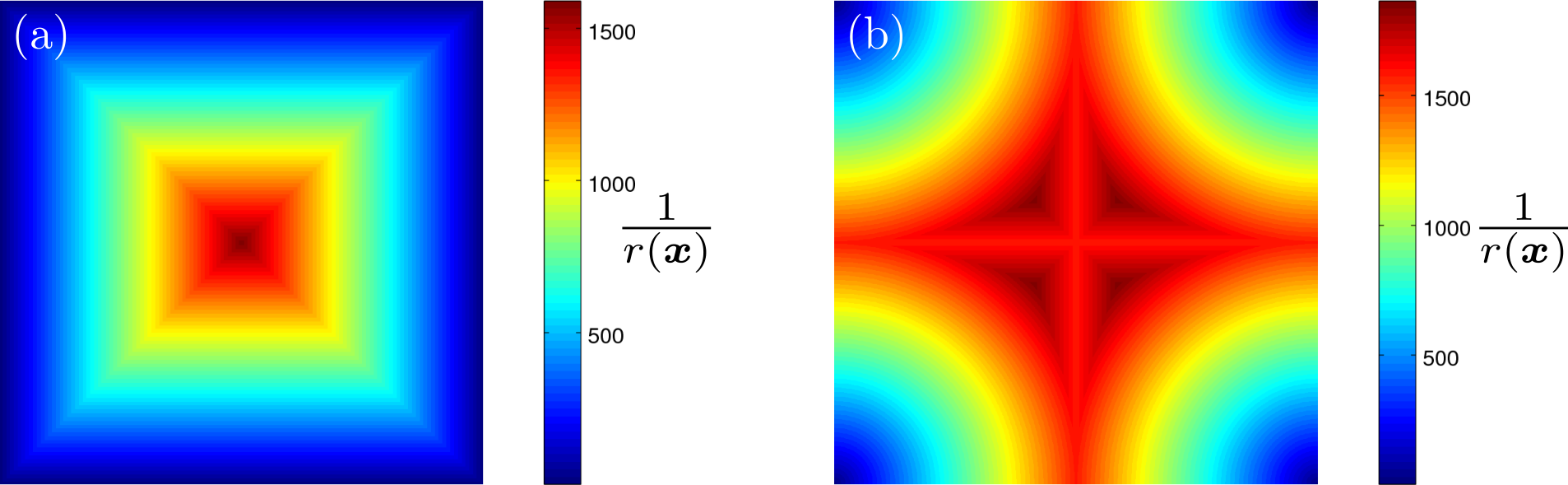
The resolution limit stated in result 3.2 is isotropic – the resolution for features along a specific direction may be higher. Figure 4(a) shows the spatially varying resolution according to the estimate (3.10) for the exemplary setting m=2m=2, K=[−12;12]2K=[-\frac{1}{2};\frac{1}{2}]^{2}, 𝔣=104\mathfrak{f}=10^{4}. Note that the maximum resolution max𝒙∈K⁡1/r⁡(𝒙)=¯​𝔣\max_{\boldsymbol{x}\in K}1/r(\boldsymbol{x})=\lower 3.87495pt\hbox{$\mathchar 22$}\mkern-8.0mu\mathfrak{f} coincides with predictions according to Abbe’s diffraction limit if the detector-size defines the numerical aperture, compare [21, 15]. Interestingly, however, the resolution only attains this optimum in the very center of the FoV as it decreases towards the detector-edges.
Refer to caption
Figure 4: (a) Upper bound on the stably reconstructible local resolution 1/r⁡(𝒙)1/r(\boldsymbol{x}) in IP 1 (complex-valued images) for m=2m=2, K=[−12;12]2K=[-\frac{1}{2};\frac{1}{2}]^{2}, 𝔣=104\mathfrak{f}=10^{4} according to the estimate (3.10). (b) Same plot for IP 2, i.e. for real-valued image-reconstruction, according to the estimate (3.15).

3.3.2 Resolution for real-valued images

In the case of IP 2(a), real-valued images are to be reconstructed so that complex-valued Gaussian wave-packets are no longer admissible perturbations. Accordingly, we study real-valued wave-packets. Such signals are given by a superposition of two Gaussian wave-packets with wavevectors 𝝃\boldsymbol{\xi} and −𝝃-\boldsymbol{\xi}:

h𝝃,𝒂real​(𝒙)\displaystyle h_{\boldsymbol{\xi},\boldsymbol{a}}^{\textup{real}}(\boldsymbol{x}) :=cos⁡(𝝃⋅(𝒙−𝒂)+β)​pσ​(𝒙−𝒂)\displaystyle:=\cos\big(\boldsymbol{\xi}\cdot(\boldsymbol{x}-\boldsymbol{a})+\beta\big)p_{\sigma}(\boldsymbol{x}-\boldsymbol{a})
=Re​(ei​β​h𝝃,𝒂​(𝒙))=12​(ei​β​h𝝃,𝒂​(𝒙)+e−i​β​h−𝝃,𝒂​(𝒙))\displaystyle=\textup{Re}\left(\text{{e}}^{\text{{i}}\beta}h_{\boldsymbol{\xi},\boldsymbol{a}}(\boldsymbol{x})\right)={\textstyle\frac{1}{2}}\left(\text{{e}}^{\text{{i}}\beta}h_{\boldsymbol{\xi},\boldsymbol{a}}(\boldsymbol{x})+\text{{e}}^{-\text{{i}}\beta}h_{-\boldsymbol{\xi},\boldsymbol{a}}(\boldsymbol{x})\right) (3.11)

for 𝒙,𝝃,𝒂∈ℝm,β∈[0;2​π)\boldsymbol{x},\boldsymbol{\xi},\boldsymbol{a}\in\mathbb{R}^{m},\beta\in[0;2\pi). Using (3.6) and linearity of the Fresnel-propagator, an analytical propagation formula is obtained for h𝝃,𝒂realh_{\boldsymbol{\xi},\boldsymbol{a}}^{\textup{real}}:

𝒟⁡(h𝝃,𝒂real)​(𝒙)\displaystyle\mathcal{D}\big(h_{\boldsymbol{\xi},\boldsymbol{a}}^{\textup{real}}\big)(\boldsymbol{x}) =ei​β2​𝒟​(h𝝃,𝒂)​(𝒙)+e−i​β2​𝒟​(h−𝝃,𝒂)​(𝒙)\displaystyle=\frac{\text{{e}}^{\text{{i}}\beta}}{2}\mathcal{D}\left(h_{\boldsymbol{\xi},\boldsymbol{a}}\right)(\boldsymbol{x})+\frac{\text{{e}}^{-\text{{i}}\beta}}{2}\mathcal{D}\left(h_{-\boldsymbol{\xi},\boldsymbol{a}}\right)(\boldsymbol{x})
=ei​β2​ν𝝃​(𝒙−𝒂−𝝃/𝔣)​pσ~​(𝒙−𝒂−𝝃/𝔣)+e−i​β2​ν−𝝃​(𝒙−𝒂+𝝃/𝔣)​pσ~​(𝒙−𝒂+𝝃/𝔣)\displaystyle=\frac{\text{{e}}^{\text{{i}}\beta}}{2}\nu_{\boldsymbol{\xi}}\left(\boldsymbol{x}-\boldsymbol{a}-\boldsymbol{\xi}/\mathfrak{f}\right)p_{\tilde{\sigma}}(\boldsymbol{x}-\boldsymbol{a}-\boldsymbol{\xi}/\mathfrak{f})+\frac{\text{{e}}^{-\text{{i}}\beta}}{2}\nu_{-\boldsymbol{\xi}}\left(\boldsymbol{x}-\boldsymbol{a}+\boldsymbol{\xi}/\mathfrak{f}\right)p_{\tilde{\sigma}}(\boldsymbol{x}-\boldsymbol{a}+\boldsymbol{\xi}/\mathfrak{f}) (3.12)
Refer to caption
Figure 5: Analogue of fig. 3 for a real-valued wave-packet h𝝃,𝒙0realh_{\boldsymbol{\xi},\boldsymbol{x}_{0}}^{\textup{real}}. Upon Fresnel-propagation, such split up into two wave-packets that laterally propagate along opposite directions ±𝝃\pm\boldsymbol{\xi}. Consequently, the induced data contrast 𝒟⁡(h𝝃,𝒙0real)|K\mathcal{D}(h_{\boldsymbol{\xi},\boldsymbol{x}_{0}}^{\textup{real}})|_{K} is non-negligible under milder conditions than in the complex-valued case. For details, see text.

The analytical solution (3.12) reveals surprising features of the propagated signal: upon propagation, the wave-packet splits up into two packets propagating into opposite directions ±𝝃\pm\boldsymbol{\xi} as visualized in fig. 5. This has important consequences in terms of stability: if an object h∈L2​(Ω,ℝ)h\in L^{2}(\Omega,\mathbb{R}) is perturbed by a real-valued wave-packet h𝝃,𝒙realh_{\boldsymbol{\xi},\boldsymbol{x}}^{\textup{real}} at some point 𝒙∈K\boldsymbol{x}\in K, then this perturbation manifests non-negligibly in the data 𝒟⁡(h+h𝝃,𝒙real)|K\mathcal{D}(h+h_{\boldsymbol{\xi},\boldsymbol{x}}^{\textup{real}})|_{K} as long as either of the two wave-packets remains within the field-of-view KK. For a point 𝒙∈K\boldsymbol{x}\in K and a direction 𝒏\boldsymbol{n}, we therefore introduce the following distance-measure:

distsym𝒏(𝒙,∂K)\displaystyle\dist\!_{\textup{sym}}^{\boldsymbol{n}}(\boldsymbol{x},\partial K) =inf{y≥0:𝒙+y​𝒏∉K​ and ​𝒙−y​𝒏∉K}\displaystyle=\inf\left\{y\geq 0:\boldsymbol{x}+y\boldsymbol{n}\notin K\textup{ and }\boldsymbol{x}-y\boldsymbol{n}\notin K\right\} (3.13)
distsym(𝒙,∂K)\displaystyle\dist\!_{\textup{sym}}(\boldsymbol{x},\partial K) =inf|𝒏|=1distsym𝒏(𝒙,∂K).\displaystyle=\inf_{|\boldsymbol{n}|=1}\dist\!_{\textup{sym}}^{\boldsymbol{n}}(\boldsymbol{x},\partial K). (3.14)

distsym𝒏(𝒙,∂K)\dist\!_{\textup{sym}}^{\boldsymbol{n}}(\boldsymbol{x},\partial K) gives the larger length of the two line-segments {𝒙±y​𝒏:y≥0}∩K\{\boldsymbol{x}\pm y\boldsymbol{n}:y\geq 0\}\cap K, which connect 𝒙\boldsymbol{x} with the boundary of ∂K\partial K along 𝒏\boldsymbol{n}. In view of wave-packets, the interpretation is simple: for 𝒙,𝝃∈ℝm\boldsymbol{x},\boldsymbol{\xi}\in\mathbb{R}^{m}, the centers of both propagating wave-packets forming 𝒟⁡(h𝝃,𝒙real)\mathcal{D}(h_{\boldsymbol{\xi},\boldsymbol{x}}^{\textup{real}}) lie outside KK if and only if distsym𝝃/|𝝃|(𝒙,∂K)<|𝝃|/𝔣\dist\!_{\textup{sym}}^{\boldsymbol{\xi}/|\boldsymbol{\xi}|}(\boldsymbol{x},\partial K)<|\boldsymbol{\xi}|/\mathfrak{f}. Hence, the following relations hold true:

  • 𝟏\boldsymbol{1}

    For all wave-packets h𝝃,𝒙realh_{\boldsymbol{\xi},\boldsymbol{x}}^{\textup{real}} with |𝝃|<𝔣​distsym(𝒙,∂K)|\boldsymbol{\xi}|<\mathfrak{f}\dist\!_{\textup{sym}}(\boldsymbol{x},\partial K), the center of one of the propagating wave-packets lies within KK.

  • 𝟐\boldsymbol{2}

    For all frequencies ξ>𝔣​distsym(𝒙,∂K)\xi>\mathfrak{f}\dist\!_{\textup{sym}}(\boldsymbol{x},\partial K), there exists a wave-packet h𝝃,𝒙realh_{\boldsymbol{\xi},\boldsymbol{x}}^{\textup{real}} with |𝝃|=ξ|\boldsymbol{\xi}|=\xi, such that the center of both wave-packets lie outside of KK.

Accordingly, the quantity distsym(𝒙,∂K)\dist\!_{\textup{sym}}(\boldsymbol{x},\partial K) yields an upper bound for the local resolution in the real-valued setting:

Result 3.3 (Resolution limit for real-valued image reconstruction).

For KK convex and Ω⊂K\Omega\subset K, stable reconstruction in IP 2 can only be achieved down to a local resolution limit

1/r⁡(𝒙)≲𝔣​distsym​(𝒙,∂K)πfor all𝒙∈Ω,\displaystyle 1/r(\boldsymbol{x})\lesssim\frac{\mathfrak{f}\dist\!_{\textup{sym}}(\boldsymbol{x},\partial K)}{\pi}\;\;\;\;\;\text{for all}\;\;\;\;\;\boldsymbol{x}\in\Omega, (3.15)

where r⁡(𝐱)r(\boldsymbol{x}) denotes the smallest resolvable feature-size of the image φ\varphi at position 𝐱\boldsymbol{x}.

For m=2m=2, K=[−12;12]2K=[-\frac{1}{2};\frac{1}{2}]^{2}, distsym\dist\!_{\textup{sym}} can be evaluated analytically:

distsym((x1,x2),∂K)=min⁡{((12−|x1|)2+(12−|x2|)2)12,minj∈{1,2}⁡max±​12±xj}\displaystyle\dist\!_{\textup{sym}}\big((x_{1},x_{2}),\partial K\big)=\min\Big\{\Big(\big({\textstyle\frac{1}{2}}-|x_{1}|\big)^{2}+\big({\textstyle\frac{1}{2}}-|x_{2}|\big)^{2}\Big)^{\frac{1}{2}},\min_{j\in\{1,2\}}\max_{\pm}{\textstyle\frac{1}{2}}\pm x_{j}\Big\} (3.16)

The resulting spatially varying resolution for 𝔣=104\mathfrak{f}=10^{4} is plotted in fig. 4(b). Notably, the maximum resolution is attained slightly off-center and is higher than in complex-valued case, compare fig. 4(a). Moreover, a high resolution 1/r≥10001/r\geq 1000 is obtained within a much larger subdomain of the field of view KK. Most prominently, the resolution in fig. 4(b) even remains large near the detector boundary – except for the corners of KK. Yet, the maximum resolution remains essentially bounded by max𝒙∈K⁡1/r⁡(𝒙)≲¯​𝔣\max_{\boldsymbol{x}\in K}1/r(\boldsymbol{x})\lesssim\lower 3.87495pt\hbox{$\mathchar 22$}\mkern-8.0mu\mathfrak{f}.

4 Locality estimates for complex-valued objects

The goal of the subsequent sections is to complement the (potentially) optimistic resolution estimates from §\lx@sectionsign3 with worst-case bounds. Accordingly, we aim to prove that stable image reconstruction can indeed be achieved down to a certain resolution. Note that this is necessarily more involved than the preceding analysis because stability has to be proven with respect to general perturbations instead of considering just a special class like Gaussian wave-packets.

4.1 Basic idea and preliminaries

The principal difficulty in proving stability-estimates for bounded detection domains K⊂ℝmK\subset\mathbb{R}^{m} lies in the pronounced non-locality of the Fresnel-propagator: according to (P2), it is given by a convolution with a kernel k𝔣​(𝒙)∝exp⁡(i​𝔣​𝒙/2)k_{\mathfrak{f}}(\boldsymbol{x})\propto\exp(\text{{i}}\mathfrak{f}\boldsymbol{x}/2) that shows no spatial decay whatsoever! Hence, Fresnel-propagation may transport object-information over arbitrary lateral distances in principle, i.e. features of the imaged object h∈L2​(Ω)h\in L^{2}(\Omega) with Ω⊂K\Omega\subset K may manifest far outside the field-of-view KK in the diffraction data 𝒟⁡(h)\mathcal{D}(h). In addition to this non-locality in real-space, any restriction to K⊊ℝmK\subsetneq\mathbb{R}^{m} breaks the translational invariance of 𝒟\mathcal{D} and thus its diagonality, i.e. locality, in Fourier-space.

On the other hand, it has been seen in §\lx@sectionsign3 that the distance, by which object-information is transported laterally, depends on the spatial frequencies of the signal. Accordingly, locality might be established by restricting to lower frequencies, i.e. to sufficiently smooth objects.

The principal idea of the subsequent analysis is to decompose the convolution kernel k𝔣k_{\mathfrak{f}} into an inner, local part, and an outer non-local part:

k𝔣=k𝔣|P+k𝔣|Pcfor someP⊂ℝm.\displaystyle k_{\mathfrak{f}}=k_{\mathfrak{f}}|_{P}+k_{\mathfrak{f}}|_{P^{\textup{c}}}\;\;\;\;\;\text{for some}\;\;\;\;\;P\subset\mathbb{R}^{m}. (4.1)

For an object h∈L2​(Ω)h\in L^{2}(\Omega) supported in Ω⊂K⊂ℝm\Omega\subset K\subset\mathbb{R}^{m} and a suitably chosen PP, the wave-field leaked outside KK depends only on the outer part: 𝒟⁡(h)|Kc=(k𝔣∗h)|Kc=(k𝔣|Pc∗h)|Kc\mathcal{D}(h)|_{K^{\textup{c}}}=(k_{\mathfrak{f}}\ast h)|_{K^{\textup{c}}}=(k_{\mathfrak{f}}|_{P^{\textup{c}}}\ast h)|_{K^{\textup{c}}}. This implies estimates of the form ‖𝒟⁡(h)|Kc‖≤‖k𝔣|Pc∗h‖\|\mathcal{D}(h)|_{K^{\textup{c}}}\|\leq\|k_{\mathfrak{f}}|_{P^{\textup{c}}}\ast h\|, which are diagonal in Fourier-space and thus simple to interpret as the norm of a filtered object.

Notation: indicator functions

For a set A⊂ℝmA\subset\mathbb{R}^{m}, let 𝟏A:ℝm→ℝ\boldsymbol{1}_{A}:\mathbb{R}^{m}\to\mathbb{R} be defined by 𝟏A​(𝒙)=1\boldsymbol{1}_{A}(\boldsymbol{x})=1 if 𝒙∈A\boldsymbol{x}\in A and 𝟏A​(𝒙)=0\boldsymbol{1}_{A}(\boldsymbol{x})=0 otherwise.

4.2 Principal leakage estimates

Our principal leakage estimate is based on the insight that the frequency response of a restricted Fresnel-kernel k𝔣|Pk_{\mathfrak{f}}|_{P} is readily computable:

Lemma 4.1 (Frequency response of a restricted Fresnel-kernels).

Let P⊂ℝmP\subset\mathbb{R}^{m} be a measurable set such that 𝒟⁡(𝟏P)∈L∞​(ℝm)\mathcal{D}(\boldsymbol{1}_{P})\in L^{\infty}(\mathbb{R}^{m}) is well-defined and bounded. Let k𝔣k_{\mathfrak{f}} denote the convolution-kernel of the Fresnel-propagator. Then it holds for all h∈L2​(ℝm)h\in L^{2}(\mathbb{R}^{m}) that

ℱ⁡(k𝔣|P∗h)​(𝝃)\displaystyle\mathcal{F}\left(k_{\mathfrak{f}}|_{P}\ast h\right)(\boldsymbol{\xi}) =m𝔣(𝝃)⋅𝒟(𝟏P)(𝝃/𝔣)⋅ℱ(h)(𝝃)for almost all𝝃∈ℝm\displaystyle=m_{\mathfrak{f}}(\boldsymbol{\xi})\cdot\mathcal{D}(\boldsymbol{1}_{P})(\boldsymbol{\xi}/\mathfrak{f})\cdot\mathcal{F}\left(h\right)(\boldsymbol{\xi})\;\;\;\;\;\text{for almost all}\;\;\;\;\;\boldsymbol{\xi}\in\mathbb{R}^{m} (4.2)

and in particular for any measurable set A⊂ℝmA\subset\mathbb{R}^{m}:

‖(k𝔣|P∗h)|A‖\displaystyle\left\|(k_{\mathfrak{f}}|_{P}\ast h)|_{A}\right\| ≤‖𝒟(𝟏P)(⋅/𝔣)⋅ℱ(h)‖.\displaystyle\leq\left\|\mathcal{D}(\boldsymbol{1}_{P})(\cdot/\mathfrak{f})\cdot\mathcal{F}\left(h\right)\right\|. (4.3)

Proof.

By the assumption 𝒟⁡(𝟏P)∈L∞​(ℝm)\mathcal{D}(\boldsymbol{1}_{P})\in L^{\infty}(\mathbb{R}^{m}), both sides of the equation (4.2) are continuous in hh with respect to the L2L^{2}-norm. Hence, it is sufficient to prove the claim for Schwartz-functions h∈𝒮⁡(ℝm)h\in\mathscr{S}(\mathbb{R}^{m}) by denseness of these in L2​(ℝm)L^{2}(\mathbb{R}^{m}).

For h∈𝒮⁡(ℝm)h\in\mathscr{S}(\mathbb{R}^{m}), the convolution k𝔣|P∗hk_{\mathfrak{f}}|_{P}\ast h is well-defined in a pointwise sense but can also be regarded as convolution between a Schwartz-function and a tempered distribution k𝔣|P∈𝒮​(ℝm)′k_{\mathfrak{f}}|_{P}\in\mathscr{S}(\mathbb{R}^{m})^{\prime}. Accordingly, the convolution theorem holds, i.e.

ℱ((𝟏P⋅k𝔣)∗h)=(2π)−m/2ℱ(𝟏P⋅k𝔣)⋅ℱ(h)\displaystyle\mathcal{F}\left((\boldsymbol{1}_{P}\cdot k_{\mathfrak{f}})\ast h\right)=(2\pi)^{-m/2}\mathcal{F}(\boldsymbol{1}_{P}\cdot k_{\mathfrak{f}})\cdot\mathcal{F}(h) (4.4)

in a distributional sense. Recalling that the alternate form of the Fresnel-propagator (P3) remains valid for tempered distributions, we get

ℱ⁡(𝟏P⋅k𝔣)=u0​𝔣m2​ℱ​(𝟏P⋅n𝔣)\displaystyle\mathcal{F}(\boldsymbol{1}_{P}\cdot k_{\mathfrak{f}})=u_{0}\mathfrak{f}^{\frac{m}{2}}\mathcal{F}(\boldsymbol{1}_{P}\cdot n_{\mathfrak{f}}) =1n𝔣(⋅/𝔣)(u0𝔣m2n𝔣(⋅/𝔣)⋅ℱ(𝟏P⋅n𝔣)(𝔣(⋅/𝔣)))\displaystyle=\frac{1}{n_{\mathfrak{f}}\left(\cdot/\mathfrak{f}\right)}\left(u_{0}\mathfrak{f}^{\frac{m}{2}}n_{\mathfrak{f}}\left(\cdot/\mathfrak{f}\right)\cdot\mathcal{F}(\boldsymbol{1}_{P}\cdot n_{\mathfrak{f}})\left(\mathfrak{f}\left(\cdot/\mathfrak{f}\right)\right)\right)
=(P3)m𝔣⋅𝒟(𝟏P)(⋅/𝔣)\displaystyle\stackrel{{\scriptstyle\eqref{eq:FresnelPropAltForm}}}{{=}}m_{\mathfrak{f}}\cdot\mathcal{D}(\boldsymbol{1}_{P})(\cdot/\mathfrak{f}) (4.5)

Inserting (4.5) into (4.4) yields (4.2). The inequality (4.3) now follows by using unitarity of the Fourier transform along with the observations that m𝔣m_{\mathfrak{f}} has constant modulus 1 and that the restriction-operation f↦f|Af\mapsto f|_{A} is non-increasing in the L2L^{2}-norm:

‖(k𝔣|P∗h)|A‖\displaystyle\left\|(k_{\mathfrak{f}}|_{P}\ast h)|_{A}\right\| ≤‖k𝔣|P∗h‖=‖ℱ(k𝔣|P∗h)‖=(4.2)‖m𝔣⋅𝒟(𝟏P)(⋅/𝔣)⋅ℱ(h)‖\displaystyle\leq\left\|k_{\mathfrak{f}}|_{P}\ast h\right\|=\left\|\mathcal{F}(k_{\mathfrak{f}}|_{P}\ast h)\right\|\stackrel{{\scriptstyle\eqref{eq:lem-LocalFresnel-1}}}{{=}}\left\|m_{\mathfrak{f}}\cdot\mathcal{D}(\boldsymbol{1}_{P})(\cdot/\mathfrak{f})\cdot\mathcal{F}\left(h\right)\right\|
=‖𝒟(𝟏P)(⋅/𝔣)⋅ℱ(h)‖.\displaystyle=\left\|\mathcal{D}(\boldsymbol{1}_{P})(\cdot/\mathfrak{f})\cdot\mathcal{F}\left(h\right)\right\|. (4.6)

A surprising feature of lemma 4.1 is that 𝒟⁡(…)\mathcal{D}(\ldots) occurs as a factor in Fourier-space. Similar as lemma 3.1, this reveals an interesting real-space-Fourier-space-duality of the Fresnel-propagator. Using lemma 4.1, we may derive leakage estimates as outlined in §\lx@sectionsign4.1:

Theorem 4.2 (Principal leakage estimate).

Let K,Ω,Pleak⊂ℝmK,\Omega,P_{{\textup{leak}}}\subset\mathbb{R}^{m} be measurable sets such that the boundary ∂K\partial K has Lebesgue-measure zero and Ω+Pleak={𝐱+𝐲:𝐱∈Ω,𝐲∈Pleak}⊂K\Omega+P_{{\textup{leak}}}=\{\boldsymbol{x}+\boldsymbol{y}:\boldsymbol{x}\in\Omega,\boldsymbol{y}\in P_{{\textup{leak}}}\}\subset K. Moreover, let 𝒟⁡(𝟏Pleakc)∈L∞​(ℝm)\mathcal{D}(\boldsymbol{1}_{P^{\textup{c}}_{{\textup{leak}}}})\in L^{\infty}(\mathbb{R}^{m}). Then it holds for all h∈L2​(Ω)h\in L^{2}(\Omega)

‖𝒟⁡(h)|Kc‖≤‖p^leak⋅ℱ⁡(h)‖,pleak​(𝝃):=|𝒟⁡(𝟏Pleakc)​(𝝃/𝔣)|.\displaystyle\left\|\mathcal{D}\left(h\right)|_{K^{\textup{c}}}\right\|\leq\big\|\hat{p}^{{\textup{leak}}}\cdot\mathcal{F}\left(h\right)\big\|,\qquad p^{{\textup{leak}}}(\boldsymbol{\xi}):=\left|\mathcal{D}(\boldsymbol{1}_{P^{\textup{c}}_{{\textup{leak}}}})(\boldsymbol{\xi}/\mathfrak{f})\right|. (4.7)

Proof.

By a similar continuity argument as in lemma 4.1 it is sufficient to prove the claim for Schwartz-functions h∈L2​(Ω)∩𝒮⁡(ℝm)h\in L^{2}(\Omega)\cap\mathscr{S}(\mathbb{R}^{m}). Then the convolution-form (P2) of the Fresnel-propagator may be used. Hence, we have

𝒟⁡(h)|Kc\displaystyle\mathcal{D}\left(h\right)|_{K^{\textup{c}}} =(k𝔣∗h)|Kc=((𝟏Pleak⋅k𝔣)∗h)|Kc+((𝟏Pleakc⋅k𝔣)∗h)|Kc\displaystyle=\left(k_{\mathfrak{f}}\ast h\right)|_{K^{\textup{c}}}=\left(\left(\boldsymbol{1}_{P_{{\textup{leak}}}}\cdot k_{\mathfrak{f}}\right)\ast h\right)|_{K^{\textup{c}}}+\left(\left(\boldsymbol{1}_{P^{\textup{c}}_{{\textup{leak}}}}\cdot k_{\mathfrak{f}}\right)\ast h\right)|_{K^{\textup{c}}} (4.8)

According to standard results on the support of convolutions, it holds that

supp((𝟏Pleak⋅k𝔣)∗h)\displaystyle\supp\left(\left(\boldsymbol{1}_{P_{{\textup{leak}}}}\cdot k_{\mathfrak{f}}\right)\ast h\right) ⊂supp(𝟏Pleak⋅k𝔣)+supp(h)¯⊂Pleak+Ω¯⊂K¯.\displaystyle\subset{}\mkern 3.0mu\overline{\mkern-3.0mu\supp\left(\boldsymbol{1}_{P_{{\textup{leak}}}}\cdot k_{\mathfrak{f}}\right)+\supp\left(h\right)}\subset{}\mkern 3.0mu\overline{\mkern-3.0muP_{{\textup{leak}}}+\Omega}\subset{}\mkern 3.0mu\overline{\mkern-3.0muK}. (4.9)

(4.9) implies that ((𝟏Pleak⋅k𝔣)∗h)|Kc\left(\left(\boldsymbol{1}_{P_{{\textup{leak}}}}\cdot k_{\mathfrak{f}}\right)\ast h\right)|_{K^{\textup{c}}} vanishes except for possibly the boundary ∂K\partial K. As ∂K\partial K is a set of measure zero, ((𝟏Pleak⋅k𝔣)∗h)|Kc=0\left(\left(\boldsymbol{1}_{P_{{\textup{leak}}}}\cdot k_{\mathfrak{f}}\right)\ast h\right)|_{K^{\textup{c}}}=0 holds in an L2L^{2}-sense. Thus, (4.8) yields

‖𝒟⁡(h)|Kc‖\displaystyle\left\|\mathcal{D}\left(h\right)|_{K^{\textup{c}}}\right\| =‖((𝟏Pleakc⋅k𝔣)∗h)|Kc‖\displaystyle=\left\|\left(\left(\boldsymbol{1}_{P^{\textup{c}}_{{\textup{leak}}}}\cdot k_{\mathfrak{f}}\right)\ast h\right)|_{K^{\textup{c}}}\right\| (4.10)

Applying the bound (4.3) to the right-hand side of (4.10) now yields the assertion.

Theorem 4.2 bounds the leaked wave-field 𝒟⁡(h)|Kc\mathcal{D}(h)|_{K^{\textup{c}}} in terms of a filtering-operation. In order to predict in which cases leakage is small or large, we need to understand the nature of the filter-response p^leak\hat{p}^{{\textup{leak}}} that weights the Fourier-components of hh in (4.7). If Ω⊂K⊂ℝm\Omega\subset K\subset\mathbb{R}^{m}, then the largest admissible set PP in theorem 4.2 is some bounded domain containing 0, where the exact size of PP depends on the distance between Ω\Omega and ∂K\partial K. Let us assume that the size of PP is much larger than 1/𝔣121/\mathfrak{f}^{\frac{1}{2}} as will be the typical case in the following. Then the indicator-function 𝟏Pc\boldsymbol{1}_{P^{\textup{c}}} is essentially preserved upon Fresnel-propagation, i.e. 𝒟⁡(𝟏Pc)≈𝟏Pc=1−𝟏P\mathcal{D}(\boldsymbol{1}_{P^{\textup{c}}})\approx\boldsymbol{1}_{P^{\textup{c}}}=1-\boldsymbol{1}_{P} up to some oscillations near the boundary of PP. Accordingly, p^leak=𝒟(𝟏Pc)(⋅/𝔣)\hat{p}^{{\textup{leak}}}=\mathcal{D}(\boldsymbol{1}_{P^{\textup{c}}})(\cdot/\mathfrak{f}) acts as a high-pass filter, essentially damping out all Fourier-frequencies within the domain 𝔣⋅𝟏P\mathfrak{f}\cdot\boldsymbol{1}_{P}. Thus, the right-hand side of (4.7) is small for sufficiently smooth objects hh.

4.3 Explicit leakage bounds for rectangular domains

For general sets PleakP_{{\textup{leak}}}, p^leak\hat{p}^{\textup{leak}} from theorem 4.2 cannot be computed explicitly. An exception is given by rectangular domains owing to the known Fresnel-transform of the Heaviside-function θ=𝟏ℝ≥0\theta=\boldsymbol{1}_{\mathbb{R}_{\geq 0}} in terms of Fresnel-integrals [16]:

𝒟​(θ)​(x)\displaystyle\mathcal{D}(\theta)(x) =12−1−i2​(C​(−𝔣12​xπ12)+iS​(−𝔣12​xπ12))=:θ~​(𝔣12​x)\displaystyle=\frac{1}{2}-\frac{1-\text{{i}}}{2}\bigg(\textup{C}\bigg(\frac{-\mathfrak{f}^{\frac{1}{2}}x}{\pi^{\frac{1}{2}}}\bigg)+\text{{i}}\textup{S}\bigg(\frac{-\mathfrak{f}^{\frac{1}{2}}x}{\pi^{\frac{1}{2}}}\bigg)\bigg)=:\tilde{\theta}(\mathfrak{f}^{\frac{1}{2}}x)
C​(x)\displaystyle\textup{C}(x) :=∫0xcos(π2t2)dt,S(x):=∫0xsin(π2t2)dtfor allx∈ℝ\displaystyle:=\int_{0}^{x}\cos\left(\frac{\pi}{2}t^{2}\right)\,\text{{d}}t,\quad\textup{S}(x):=\int_{0}^{x}\sin\left(\frac{\pi}{2}t^{2}\right)\,\text{{d}}t\;\;\;\;\;\text{for all}\;\;\;\;\;x\in\mathbb{R} (4.11)

Note that θ~\tilde{\theta} is an entire analytic function and bounded with maxx∈ℝ⁡|θ~​(x)|≤1.171\max_{x\in\mathbb{R}}|\tilde{\theta}(x)|\leq 1.171.

By the separability- and isotropy-properties of the Fresnel-propagator, (P4) and (P5), the explicit solution generalizes to half-spaces Ha,𝒏:={𝒙∈ℝm:𝒏⋅𝒙≥a}H_{a,\boldsymbol{n}}:=\{\boldsymbol{x}\in\mathbb{R}^{m}:\boldsymbol{n}\cdot\boldsymbol{x}\geq a\} in arbitrary dimensions with a∈ℝa\in\mathbb{R} and 𝒏∈𝕊m−1={𝒙∈ℝm:|𝒏|=1}\boldsymbol{n}\in\mathbb{S}^{m-1}=\{\boldsymbol{x}\in\mathbb{R}^{m}:|\boldsymbol{n}|=1\}:

𝒟⁡(𝟏Ha,𝒏)​(𝒙)=θ~​(𝔣12​(𝒏⋅𝒙−a))for all𝒙∈ℝm.\displaystyle\mathcal{D}(\boldsymbol{1}_{H_{a,\boldsymbol{n}}})(\boldsymbol{x})=\tilde{\theta}\big(\mathfrak{f}^{\frac{1}{2}}(\boldsymbol{n}\cdot\boldsymbol{x}-a)\big)\;\;\;\;\;\text{for all}\;\;\;\;\;\boldsymbol{x}\in\mathbb{R}^{m}. (4.12)

Using linearity of 𝒟\mathcal{D}, (4.11) furthermore yields the Fresnel-transform of intervals:

𝒟​(𝟏[−Δ;Δ])​(x)\displaystyle\mathcal{D}(\boldsymbol{1}_{[-\Delta;\Delta]})(x) =𝒟(𝟏[Δ;∞))(x)−𝒟(𝟏[−Δ;∞))(x)=θ~(𝔣12(x−Δ))−θ~(𝔣12(x+Δ))\displaystyle=\mathcal{D}(\boldsymbol{1}_{[\Delta;\infty)})(x)-\mathcal{D}(\boldsymbol{1}_{[-\Delta;\infty)})(x)=\tilde{\theta}\left(\mathfrak{f}^{\frac{1}{2}}(x-\Delta)\right)-\tilde{\theta}\big(\mathfrak{f}^{\frac{1}{2}}(x+\Delta)\big)
=θ~​(𝔣12​x−𝔣Δ12)−θ~​(𝔣12​x+𝔣Δ12)=:ι~𝔣Δ​(𝔣12​x)\displaystyle=\tilde{\theta}\big(\mathfrak{f}^{\frac{1}{2}}x-\mathfrak{f}_{\Delta}^{\frac{1}{2}}\big)-\tilde{\theta}\big(\mathfrak{f}^{\frac{1}{2}}x+\mathfrak{f}_{\Delta}^{\frac{1}{2}}\big)=:\tilde{\iota}_{\mathfrak{f}_{\Delta}}(\mathfrak{f}^{\frac{1}{2}}x) (4.13)

Here, we introduced the Fresnel number associated with the lateral lengthscale Δ>0\Delta>0, 𝔣Δ:=Δ2​𝔣\mathfrak{f}_{\Delta}:=\Delta^{2}\mathfrak{f}, compare §\lx@sectionsign2.1.4. Again by the separability of the Fresnel-propagator, this generalizes to stripe-shaped domains SΔ,𝒏:={𝒙∈ℝm:−Δ≤𝒏⋅𝒙≤Δ}S_{\Delta,\boldsymbol{n}}:=\{\boldsymbol{x}\in\mathbb{R}^{m}:-\Delta\leq\boldsymbol{n}\cdot\boldsymbol{x}\leq\Delta\} and squares:

𝒟​(SΔ,𝒏)​(𝒙)\displaystyle\mathcal{D}(S_{\Delta,\boldsymbol{n}})(\boldsymbol{x}) =ι~𝔣Δ​(𝔣12​(𝒏⋅𝒙))=:ι~𝔣Δ,𝒏​(𝒙),ι~𝔣Δ,j:=ι~𝔣Δ,𝒆j\displaystyle=\tilde{\iota}_{\mathfrak{f}_{\Delta}}\left(\mathfrak{f}^{\frac{1}{2}}(\boldsymbol{n}\cdot\boldsymbol{x})\right)=:\tilde{\iota}_{\mathfrak{f}_{\Delta},\boldsymbol{n}}(\boldsymbol{x}),\qquad\tilde{\iota}_{\mathfrak{f}_{\Delta},j}:=\tilde{\iota}_{\mathfrak{f}_{\Delta},\boldsymbol{e}_{j}} (4.14)
𝒟​(𝟏[−Δ;Δ]m)​(𝒙)\displaystyle\mathcal{D}(\boldsymbol{1}_{[-\Delta;\Delta]^{m}})(\boldsymbol{x}) =∏j=1m𝒟⁡(𝟏[−Δ;Δ])​(xj)=∏j=1mι~𝔣Δ​(𝔣12​xj)=∏j=1mι~𝔣Δ,j​(𝔣12​𝒙)\displaystyle=\prod_{j=1}^{m}\mathcal{D}(\boldsymbol{1}_{[-\Delta;\Delta]})(x_{j})=\prod_{j=1}^{m}\tilde{\iota}_{\mathfrak{f}_{\Delta}}(\mathfrak{f}^{\frac{1}{2}}x_{j})=\prod_{j=1}^{m}\tilde{\iota}_{\mathfrak{f}_{\Delta},j}(\mathfrak{f}^{\frac{1}{2}}\boldsymbol{x}) (4.15)

for all 𝒙=(x1,…,xm)∈ℝm\boldsymbol{x}=(x_{1},\ldots,x_{m})\in\mathbb{R}^{m}, where 𝒆j∈ℝm\boldsymbol{e}_{j}\in\mathbb{R}^{m} denotes the jj-th unit normal vector. Finally, indicator functions of complements are simple to propagate using linearity and 𝒟⁡(1)=1\mathcal{D}(1)=1:

𝒟⁡(𝟏Ac)=𝒟⁡(1−𝟏A)=𝒟⁡(1)−𝒟⁡(𝟏A)=1−𝒟⁡(𝟏A)forA⊂ℝm.\displaystyle\mathcal{D}(\boldsymbol{1}_{A^{\textup{c}}})=\mathcal{D}(1-\boldsymbol{1}_{A})=\mathcal{D}(1)-\mathcal{D}(\boldsymbol{1}_{A})=1-\mathcal{D}(\boldsymbol{1}_{A})\;\;\;\;\;\text{for}\;\;\;\;\;A\subset\mathbb{R}^{m}. (4.16)

Using the formulas derived above, we can explicitly write down the filter from theorem 4.2 for the important special case of square domains:

Corollary 4.3 (Leakage bound for square domains).

Let K=[−12;12]mK=[-\frac{1}{2};\frac{1}{2}]^{m} and Ω=[−12+Δ;12−Δ]m\Omega=[-\frac{1}{2}+\Delta;\frac{1}{2}-\Delta]^{m} for some 0<Δ<120<\Delta<\frac{1}{2}. Then it holds for all h∈L2​(Ω)h\in L^{2}(\Omega)

‖𝒟⁡(h)|Kc‖≤‖p^□,𝔣,𝔣Δleak⋅ℱ⁡(h)‖,p^□,𝔣,𝔣Δleak​(𝝃)\displaystyle\left\|\mathcal{D}\left(h\right)|_{K^{\textup{c}}}\right\|\leq\big\|\hat{p}^{{\textup{leak}}}_{\Box,\mathfrak{f},\mathfrak{f}_{\Delta}}\cdot\mathcal{F}(h)\big\|,\qquad\hat{p}^{{\textup{leak}}}_{\Box,\mathfrak{f},\mathfrak{f}_{\Delta}}(\boldsymbol{\xi}) :=|1−∏j=1mι~𝔣Δ,j​(𝝃/𝔣12)|,𝝃∈ℝm\displaystyle:=\bigg|1-\prod_{j=1}^{m}\tilde{\iota}_{\mathfrak{f}_{\Delta},j}(\boldsymbol{\xi}/\mathfrak{f}^{\frac{1}{2}})\bigg|,\quad\boldsymbol{\xi}\in\mathbb{R}^{m} (4.17)

Proof.

If we set Pleak:=[−Δ;Δ]mP_{{\textup{leak}}}:=[-\Delta;\Delta]^{m}, the assumptions of theorem 4.2 are satisfied. The expression for the filter in (4.17) follows by using (4.15) along with (4.16).

Refer to caption
Figure 6: Plot of the leakage-filters for square-domains from (a) Corollary 4.3 and (b) theorem 4.4 for m=1m=1 dimensions and 𝔣Δ=100\mathfrak{f}_{\Delta}=100.

The filter-response p^□,𝔣,𝔣Δleak\hat{p}^{{\textup{leak}}}_{\Box,\mathfrak{f},\mathfrak{f}_{\Delta}} from Corollary 4.3 is plotted in fig. 6(a) for an exemplary 1D-setting. It can be seen to be a high-pass filter of width ≈2​(𝔣⋅𝔣Δ)1/2=2​𝔣​Δ\approx 2(\mathfrak{f}\cdot\mathfrak{f}_{\Delta})^{1/2}=2\mathfrak{f}\Delta in Fourier-space. Note that this width is in perfect agreement with the expected cut-off frequency from the Gaussian wave-packet analysis in §\lx@sectionsign3.3.1 for the considered distance dist(Ω,∂K)=Δ\dist(\Omega,\partial K)=\Delta between object-domain and detector-boundary. However, p^□,𝔣,𝔣Δleak\hat{p}^{{\textup{leak}}}_{\Box,\mathfrak{f},\mathfrak{f}_{\Delta}} is heavily oscillatory on fine scales and is not everywhere ≤1\leq 1, although this would be reasonable by unitarity of the Fresnel-propagator. Another drawback of the filter-response in (4.17) is that it varies in a non-trivial manner in higher dimensions.

Both the oscillatory behavior and the complicated high-dimensional structure can be resolved by exploiting the simple rectangular geometry to obtain an alternative filter:

Theorem 4.4 (Leakage bound for square domains with simplified filter).

Within the setting of Corollary 4.3, it holds for all h∈L2​(Ω)h\in L^{2}(\Omega)

‖𝒟⁡(h)|Kc‖\displaystyle\left\|\mathcal{D}\left(h\right)|_{K^{\textup{c}}}\right\| ≤‖p^𝔣,𝔣Δleak⋅ℱ⁡(h)‖,p^𝔣,𝔣Δleak​(𝝃):=(∑j=1m|η~𝔣Δ​(𝔣−12​𝒆j⋅𝝃)|2)12\displaystyle\leq\big\|\hat{p}^{{\textup{leak}}}_{\mathfrak{f},\mathfrak{f}_{\Delta}}\cdot\mathcal{F}(h)\big\|,\qquad\hat{p}^{{\textup{leak}}}_{\mathfrak{f},\mathfrak{f}_{\Delta}}(\boldsymbol{\xi}):=\bigg(\sum_{j=1}^{m}\left|\tilde{\eta}_{\mathfrak{f}_{\Delta}}\left(\mathfrak{f}^{-\frac{1}{2}}\boldsymbol{e}_{j}\cdot\boldsymbol{\xi}\right)\right|^{2}\bigg)^{\frac{1}{2}} (4.18)
η~𝔣Δ​(x)\displaystyle\tilde{\eta}_{\mathfrak{f}_{\Delta}}(x) :=(|θ~​(x−𝔣Δ12)|2+|θ~​(−x−𝔣Δ12)|2)12\displaystyle:=\big(\big|\tilde{\theta}(x-\mathfrak{f}_{\Delta}^{\frac{1}{2}})\big|^{2}+\big|\tilde{\theta}(-x-\mathfrak{f}_{\Delta}^{\frac{1}{2}})\big|^{2}\big)^{\frac{1}{2}} (4.19)

where 𝐞j\boldsymbol{e}_{j} denotes the unit normal vector along the jj-th dimension.

Proof.

Let h∈L2​(Ω)h\in L^{2}(\Omega). If we define the half-spaces Hj,±:=ℝj−1×±[−12;∞)×ℝm−jH_{j,\pm}:=\mathbb{R}^{j-1}\times\pm[-\frac{1}{2};\infty)\times\mathbb{R}^{m-j}, then it holds that Kc=⋃j=1,±mHj,±cK^{\textup{c}}=\bigcup_{j=1,\pm}^{m}H_{j,\pm}^{\textup{c}}. Thus,

‖𝒟⁡(h)|Kc‖2≤∑±,j=1m‖𝒟⁡(h)|Hj,±‖2\displaystyle\left\|\mathcal{D}\left(h\right)|_{K^{\textup{c}}}\right\|^{2}\leq\sum_{\pm,j=1}^{m}\left\|\mathcal{D}(h)|_{H_{j,\pm}}\right\|^{2} (4.20)

Upon setting K~:=Hj,±\tilde{K}:=H_{j,\pm} and Pleak:=ℝj−1×±[−Δ;∞)×ℝm−jP_{{\textup{leak}}}:=\mathbb{R}^{j-1}\times\pm[-\Delta;\infty)\times\mathbb{R}^{m-j}, theorem 4.2 is applicable so that each of the squared norms on the right-hand side (4.20) can be bounded via (4.7):

‖𝒟⁡(h)|Hj,±‖2\displaystyle\left\|\mathcal{D}(h)|_{H_{j,\pm}}\right\|^{2} ≤⟨ℱ⁡(h),|p^𝔣,𝔣Δ,j,±leak|2⋅ℱ⁡(h)⟩\displaystyle\leq\big\langle\mathcal{F}(h),|\hat{p}^{{\textup{leak}}}_{\mathfrak{f},\mathfrak{f}_{\Delta},j,\pm}|^{2}\cdot\mathcal{F}(h)\big\rangle
p^𝔣,𝔣Δ,j,±leak​(𝝃)\displaystyle\hat{p}^{{\textup{leak}}}_{\mathfrak{f},\mathfrak{f}_{\Delta},j,\pm}(\boldsymbol{\xi}) =𝒟(𝟏Pleakc)(𝝃/𝔣)=(4.12)θ~(±𝔣−12𝒆j⋅𝝃−𝔣Δ12).\displaystyle=\mathcal{D}(\boldsymbol{1}_{P_{{\textup{leak}}}^{\textup{c}}})(\boldsymbol{\xi}/\mathfrak{f})\stackrel{{\scriptstyle\eqref{eq:FresnelPropHalfspace}}}{{=}}\tilde{\theta}\big(\pm\mathfrak{f}^{-\frac{1}{2}}\boldsymbol{e}_{j}\cdot\boldsymbol{\xi}-\mathfrak{f}_{\Delta}^{\frac{1}{2}}\big). (4.21)

Substituting (4.21) into (4.20) and using sesqui-linearity yields the assertion.

Figure 6(b) plots the alternate filter-response p^𝔣,𝔣Δleak\hat{p}^{{\textup{leak}}}_{\mathfrak{f},\mathfrak{f}_{\Delta}} for the same 1D-setting as in fig. 6(a). The plot reveals that the filter-profiles are almost identical except that the oscillations are eliminated from the low-frequency regime. This makes it easier to derive bounds for |p^𝔣,𝔣Δleak||\hat{p}^{{\textup{leak}}}_{\mathfrak{f},\mathfrak{f}_{\Delta}}| in a given frequency-interval compared to the original filter p^□,𝔣,𝔣Δleak\hat{p}^{{\textup{leak}}}_{\Box,\mathfrak{f},\mathfrak{f}_{\Delta}}.

4.4 Stability estimates

By unitarity of the Fresnel-propagator 𝒟\mathcal{D}, upper bounds on the wave-field leaked into KcK^{\textup{c}} induce lower bounds on the contrast within the field-of-view KK, i.e. stability estimates for the reconstruction of hh from data 𝒟⁡(h)|K\mathcal{D}(h)|_{K}:

Corollary 4.5 (Stability estimates for square domains).

Let K=[−12;12]mK=[-\frac{1}{2};\frac{1}{2}]^{m} and Ω=[−12+Δ;12−Δ]m\Omega=[-\frac{1}{2}+\Delta;\frac{1}{2}-\Delta]^{m} for some 0<Δ<120<\Delta<\frac{1}{2}. Then it holds for all h∈L2​(Ω)h\in L^{2}(\Omega)

‖𝒟⁡(h)|K‖2≥⟨ℱ⁡(h),(1−|p^leak|2)⋅ℱ⁡(h)⟩\displaystyle\left\|\mathcal{D}\left(h\right)|_{K}\right\|^{2}\geq\big\langle\mathcal{F}(h),\big(1-\big|\hat{p}^{{\textup{leak}}}\big|^{2}\big)\cdot\mathcal{F}(h)\big\rangle (4.22)

with p^leak∈{p^𝔣,𝔣Δleak,p^□,𝔣,𝔣Δleak}\hat{p}^{{\textup{leak}}}\in\{\hat{p}^{{\textup{leak}}}_{\mathfrak{f},\mathfrak{f}_{\Delta}},\hat{p}^{{\textup{leak}}}_{\Box,\mathfrak{f},\mathfrak{f}_{\Delta}}\} as defined in theorems 4.4 and 4.3.

Proof.

The claim follows from theorems 4.4 and 4.3 as ‖𝒟⁡(h)|K‖2=‖𝒟⁡(h)‖2−‖𝒟⁡(h)|Kc‖2\left\|\mathcal{D}\left(h\right)|_{K}\right\|^{2}=\left\|\mathcal{D}\left(h\right)\right\|^{2}-\left\|\mathcal{D}\left(h\right)|_{K^{\textup{c}}}\right\|^{2} and ‖𝒟⁡(h)‖2=⟨ℱ⁡(h),ℱ⁡(h)⟩\left\|\mathcal{D}\left(h\right)\right\|^{2}=\left\langle\mathcal{F}\left(h\right),\mathcal{F}\left(h\right)\right\rangle as 𝒟\mathcal{D} and ℱ\mathcal{F} are unitary.

Corollary 4.5 gives lower- and upper bounds on the contrast on a square detector in terms of filtering operations with explicitly known profile in Fourier-space. It is tempting to interpret the bound as the norm of a low-pass-filtered version of hh:

⟨ℱ⁡(h),(1−|p^leak|2)⋅ℱ⁡(h)⟩​“=”​‖(1−|p^leak|2)12⋅ℱ⁡(h)‖2\displaystyle\big\langle\mathcal{F}(h),\big(1-\big|\hat{p}^{{\textup{leak}}}\big|^{2}\big)\cdot\mathcal{F}(h)\big\rangle\textup{``=''}\big\|\big(1-\big|\hat{p}^{{\textup{leak}}}\big|^{2}\big)^{\frac{1}{2}}\cdot\mathcal{F}(h)\big\|^{2} (4.23)

However, this is technically not correct because |p^leak​(𝝃)||\hat{p}^{{\textup{leak}}}(\boldsymbol{\xi})| typically attains values greater than 1 at frequencies above the cut-off |𝝃|≥𝔣​Δ|\boldsymbol{\xi}|\geq\mathfrak{f}\Delta, see fig. 6. This means that the bound (4.22) indeed permits negative contrast in certain Fourier-frequencies. While this is certainly counter-intuitive from a physical point-of-view, one has to cope with this peculiarity in order to make sense of the stability estimates.

Since |p^leak||\hat{p}^{{\textup{leak}}}| is typically much smaller than 1 for low frequencies (compare fig. 6), the right-hand side of (4.22) will be positive for objects hh whose Fourier-transform ℱ⁡(h)\mathcal{F}(h) is sufficiently localized at low frequencies. Accordingly, a natural candidate for a class of functions that can be stably recovered from 𝒟⁡(h)|K\mathcal{D}\left(h\right)|_{K} would be band-limited ones, such that ℱ⁡(h)\mathcal{F}(h) vanishes above a certain maximum frequency, including all parts of the Fourier domain where 1−|p^leak|21-|\hat{p}^{{\textup{leak}}}|^{2} is negative. Importantly, however, Corollary 4.5 also assumes hh to have compact support in real-space so that ℱ⁡(h)\mathcal{F}(h) is an entire function and thus cannot vanish in any open set U⊂ℝmU\subset\mathbb{R}^{m} unless ℱ⁡(h)\mathcal{F}(h), and hence hh, is identically zero.

In general, we see that determining a stable class of objects naturally involves the classical problem of finding functions that are well-localized in real-space and Fourier-space at the same time, governed by so-called uncertainty principles. See e.g. [29, 8] for reviews on this topic. As a solution, we will restrict to objects given by B-splines, which may have a compact support and will be shown to be essentially band-limited in a suitable quantitative manner.

5 Stability estimates for spline objects

In the following, we derive stability results for objects given by multi-variate B-splines, which can be regarded as images of finite resolution. Such a restriction also makes sense from an experimentalist’s point-of-view as the finite number of detector-pixels introduce a natural discretization in any real-world XPCI setup.

5.1 Multi-variate B-splines

As a model for discretized, i.e. pixelated images, we consider spaces of jj-th order multi-variate B-splines: for a fixed resolution 1/r1/r with r>0r>0 and origin 𝒐∈[0;1)m\boldsymbol{o}\in[0;1)^{m}, we arrange nodes on a uniform Cartesian grid in 𝔾r,𝒐m:={𝒐+r​𝒋:𝒋∈ℤm}⊂ℝm\mathbb{G}_{r,\boldsymbol{o}}^{m}:=\left\{\boldsymbol{o}+r\boldsymbol{j}:\boldsymbol{j}\in\mathbb{Z}^{m}\right\}\subset\mathbb{R}^{m}: Now we define objects as linear combinations of basis-splines centered at these nodes:

𝔅k,r,𝒐m\displaystyle\mathfrak{B}_{k,r,\boldsymbol{o}}^{m} :={h:𝒙↦∑𝒋∈ℤmb𝒋Bkm(𝒙/r−𝒋−𝒐):(b𝒋)∈ℓ2(ℤm)}\displaystyle:=\bigg\{h:\boldsymbol{x}\mapsto\sum_{\boldsymbol{j}\in\mathbb{Z}^{m}}b_{\boldsymbol{j}}B_{k}^{m}(\boldsymbol{x}/r-\boldsymbol{j}-\boldsymbol{o}):(b_{\boldsymbol{j}})\in\ell^{2}(\mathbb{Z}^{m})\bigg\} (5.1a)
Bkm​(x1,…,xm)\displaystyle B_{k}^{m}(x_{1},\ldots,x_{m}) :=∏j=1mBk​(xj),Bk={B0∗Bk−1for ​k∈ℕ𝟏[−12;12)for ​k=0\displaystyle:=\prod_{j=1}^{m}B_{k}(x_{j}),\quad B_{k}=\begin{cases}B_{0}\ast B_{k-1}&\textup{for }k\in\mathbb{N}\\ \boldsymbol{1}_{[-\frac{1}{2};\frac{1}{2})}&\textup{for }k=0\end{cases} (5.1b)

For details and explicit formulas of B-splines, see for example [33, 32]. For our purposes here it is sufficient to note that supp(Bkm)=[−k+12;k+12]m\supp(B_{k}^{m})=[-\frac{k+1}{2};\frac{k+1}{2}]^{m} and Bkm∈𝒞k−1​(ℝm)B_{k}^{m}\in\mathscr{C}^{k-1}(\mathbb{R}^{m}) for k≥1k\geq 1.

5.1.1 Approximation properties

Splines interpolate values assigned on the grid nodes: for any sequence (y𝒋)∈ℓ2​(ℤm)(y_{\boldsymbol{j}})\in\ell^{2}(\mathbb{Z}^{m}) and k∈ℕ0k\in\mathbb{N}_{0}, there exists a unique spline h∈𝔅k,r,𝒐mh\in\mathfrak{B}_{k,r,\boldsymbol{o}}^{m} such that h⁡(r​𝒋+𝒐)=y𝒋h(r\boldsymbol{j}+\boldsymbol{o})=y_{\boldsymbol{j}} for all 𝒋∈ℤm\boldsymbol{j}\in\mathbb{Z}^{m} and the map (y𝒋)↦h(y_{\boldsymbol{j}})\mapsto h is continuous from ℓ2​(ℤm)\ell^{2}(\mathbb{Z}^{m}) to L2​(ℝm)L^{2}(\mathbb{R}^{m}). This is related to the fact that B-splines form a Riesz sequence [6]:

rm/2​CRiesz,km​‖(b𝒋)‖ℓ2​(ℤm)≤‖h‖≤rm/2​‖(b𝒋)‖ℓ2​(ℤm)\displaystyle r^{m/2}C_{\textup{Riesz},k}^{m}\left\|(b_{\boldsymbol{j}})\right\|_{\ell^{2}(\mathbb{Z}^{m})}\leq\left\|h\right\|\leq r^{m/2}\left\|(b_{\boldsymbol{j}})\right\|_{\ell^{2}(\mathbb{Z}^{m})} (5.2)

for some constants CRiesz,k>0C_{\textup{Riesz},k}>0 and all h=∑𝒋∈ℤmb𝒋Bkm(⋅/r−𝒋−𝒐)∈𝔅k,r,𝒐mh=\sum_{\boldsymbol{j}\in\mathbb{Z}^{m}}b_{\boldsymbol{j}}B_{k}^{m}(\cdot/r-\boldsymbol{j}-\boldsymbol{o})\in\mathfrak{B}_{k,r,\boldsymbol{o}}^{m}. The Riesz-sequence-property ensures stability of the approximation of functions by B-splines.

5.1.2 Separability

According to their definition in (5.1), B-splines exhibit a separable structure: for any h∈𝔅k,r,𝒐mh\in\mathfrak{B}_{k,r,\boldsymbol{o}}^{m}, 1≤j≤m1\leq j\leq m and 𝒙<j∈ℝj−1,𝒙>j∈ℝm−j\boldsymbol{x}_{<j}\in\mathbb{R}^{j-1},\boldsymbol{x}_{>j}\in\mathbb{R}^{m-j} fixed, it holds that h(𝒙<j,𝒙>j):xj↦h⁡(𝒙<j,xj,𝒙>j)∈𝔅k,r,𝒐1h_{(\boldsymbol{x}_{<j},\boldsymbol{x}_{>j})}:x_{j}\mapsto h(\boldsymbol{x}_{<j},x_{j},\boldsymbol{x}_{>j})\in\mathfrak{B}_{k,r,\boldsymbol{o}}^{1}. In other words, multi-variate B-splines are one-dimensional B-splines along each coordinate dimension.

5.2 Quasi-band-limitation of B-splines

Our interest in B-splines is mainly due to their property of being quasi band-limited. As the following estimate of this quasi-band-limitation is slightly off-topic and lengthy to derive, its proof is given in appendix B.

Theorem 5.1 (Quasi-band-limitation of univariate B-splines).

Let k∈ℕ0k\in\mathbb{N}_{0}, r>0r>0, Ξr:=[−πr;πr]\Xi_{r}:=[-\frac{\pi}{r};\frac{\pi}{r}] and ν≥1\nu\geq 1. Then it holds that

‖ℱ⁡(h)|(ν​Ξr)c‖\displaystyle\left\|\mathcal{F}(h)|_{(\nu\Xi_{r})^{\textup{c}}}\right\| ≤Cband(k,ν)‖ℱ(h)‖for allh∈𝔅k,r,𝒐1,\displaystyle\leq C_{\textup{band}}(k,\nu)\left\|\mathcal{F}(h)\right\|\;\;\;\;\;\text{for all}\;\;\;\;\;h\in\mathfrak{B}_{k,r,\boldsymbol{o}}^{1}, (5.3)

where the constant Cband​(k,ν)<1C_{\textup{band}}(k,\nu)<1 is given by

Cband​(k,ν)2\displaystyle C_{\textup{band}}(k,\nu)^{2} =cband​(k,ν)1+cband​(k,ν),cband​(k,ν)=cband,0​(k,ν)+∑n=⌈(ν−1)/2⌉∞2(2​n+1)2​(k+1)\displaystyle=\frac{c_{\textup{band}}(k,\nu)}{1+c_{\textup{band}}(k,\nu)},\quad c_{\textup{band}}(k,\nu)=c_{\textup{band},0}(k,\nu)+\!\sum_{n=\lceil(\nu-1)/2\rceil}^{\infty}\frac{2}{\left(2n+1\right)^{2(k+1)}}
cband,0​(k,ν)\displaystyle c_{\textup{band},0}(k,\nu) =max⁡{max⁡{ν~,0}2​(k+1)(ν+2​ν~)2​(k+1)+max⁡{ν~,0}2​(k+1)ν2​(k+1)−1ν¯2​(k+1), 0}\displaystyle=\max\bigg\{\frac{\max\{\tilde{\nu},0\}^{2(k+1)}}{\left(\nu+2\tilde{\nu}\right)^{2(k+1)}}+\frac{\max\{\tilde{\nu},0\}^{2(k+1)}}{\nu^{2(k+1)}}-\frac{1}{\bar{\nu}^{2(k+1)}},\;0\bigg\} (5.4)

where ⌈⋅⌉\lceil\cdot\rceil is the “round up”-operation, ν¯:=1+2​⌈(ν−1)/2⌉\bar{\nu}:=1+2\lceil(\nu-1)/2\rceil and ν~:=ν¯−ν−1\tilde{\nu}:=\bar{\nu}-\nu-1.

Conversely, for any ν<1\nu<1, there exists an h∈𝔅k,r,𝐨1h\in\mathfrak{B}_{k,r,\boldsymbol{o}}^{1} such that ℱ⁡(h)|(ν​Ξr)c=ℱ⁡(h)\mathcal{F}(h)|_{(\nu\Xi_{r})^{\textup{c}}}=\mathcal{F}(h), i.e. no estimate of the form (5.3) can hold true for any constant Cband​(k,ν)<1C_{\textup{band}}(k,\nu)<1.

Refer to caption
Figure 7: Semi-logarithmic plot of the quasi-band-limitation constant Cband​(k,ν)C_{\textup{band}}(k,\nu) from theorem 5.1 for different spline-orders kk.

The constant Cband​(k,ν)C_{\textup{band}}(k,\nu) in (5.3) may be readily evaluated by computing the infinite series in (5.4) via known analytical formulas. In fig. 7, Cband​(k,ν)C_{\textup{band}}(k,\nu) is plotted against ν\nu for different spline-orders k=0,1,3,5,7k=0,1,3,5,7. It can be seen that the bound Cband​(k,ν)C_{\textup{band}}(k,\nu) drops discontinuously from 1 to ≈2−1/2\approx 2^{-1/2} at ν=1\nu=1 and then decreases exponentially until ν≈1.5\nu\approx 1.5, where the decrease is sharper for higher spline-orders kk. For ν∈[1.5;3]\nu\in[1.5;3], the value of Cband​(k,ν)C_{\textup{band}}(k,\nu) stagnates before it continues to decrease within the interval [3;3.5][3;3.5] and so on.

By exploiting the separable structure of B-splines discussed in §\lx@sectionsign5.1.2, the 1D-result in theorem 5.1 may be easily generalized to higher dimensions:

Theorem 5.2 (Quasi-band-limitation of multivariate B-splines).

Let k∈ℕ0k\in\mathbb{N}_{0}, r>0r>0, ν≥1\nu\geq 1, Ξr:=[−πr;πr]m\Xi_{r}:=[-\frac{\pi}{r};\frac{\pi}{r}]^{m} and Ξr,j:=ℝj−1×[−πr;πr]×ℝm−j\Xi_{r,j}:=\mathbb{R}^{j-1}\times[-\frac{\pi}{r};\frac{\pi}{r}]\times\mathbb{R}^{m-j}. Then it holds that

‖ℱ⁡(h)|(ν​Ξr,j)c‖\displaystyle\big\|\mathcal{F}(h)|_{(\nu\Xi_{r,j})^{\textup{c}}}\big\| ≤Cband​(k,ν)​‖ℱ⁡(h)‖for all​     1≤j≤m,\displaystyle\leq C_{\textup{band}}(k,\nu)\left\|\mathcal{F}(h)\right\|\qquad\qquad\qquad\quad\;\;\;\;\;\text{for all}\;\;\;\;\;1\leq j\leq m, (5.5)
‖ℱ⁡(h)|(ν​Ξr)c‖\displaystyle\big\|\mathcal{F}(h)|_{(\nu\Xi_{r})^{\textup{c}}}\big\| ≤(1−(1−Cband(k,ν)2)m)12‖ℱ(h)‖for allh∈𝔅k,r,𝒐m\displaystyle\leq\left(1-\left(1-C_{\textup{band}}(k,\nu)^{2}\right)^{m}\right)^{\frac{1}{2}}\left\|\mathcal{F}(h)\right\|\;\;\;\;\;\text{for all}\;\;\;\;\;h\in\mathfrak{B}_{k,r,\boldsymbol{o}}^{m} (5.6)

5.3 Stability estimates

In the language of regularization theory, the transition to finitely sampled B-spline objects corresponds to imposing a (very strong) source condition. Similarly as proven in [1, 4] for other severely ill-posed problems, such a “finite-resolution” source condition enables Lipschitz-stability estimates for image-reconstruction from truncated Fresnel-data. This is seen by combining the quasi-band-limitation results from §\lx@sectionsign5.2 with the leakage estimates from §\lx@sectionsign4.3:

Theorem 5.3 (Stability estimate for spline-objects).

Let K=[−12;12]mK=[-\frac{1}{2};\frac{1}{2}]^{m} and Ω=[−12+Δ;12−Δ]m\Omega=[-\frac{1}{2}+\Delta;\frac{1}{2}-\Delta]^{m} for 0<Δ<120<\Delta<\frac{1}{2}. Let 𝔣Δ:=Δ2​𝔣\mathfrak{f}_{\Delta}:=\Delta^{2}\mathfrak{f} and 𝔣r:=r2​𝔣\mathfrak{f}_{r}:=r^{2}\mathfrak{f} denote the Fresnel numbers associated with the length-scales Δ\Delta and rr, respectively (compare §\lx@sectionsign2.1.4). Furthermore, let ν≥1\nu\geq 1 and Ξ:=[−νπ/𝔣r1/2;νπ/𝔣r1/2]\Xi:=[-\nu\pi/\mathfrak{f}_{r}^{1/2};\nu\pi/\mathfrak{f}_{r}^{1/2}]. Then it holds that

‖𝒟⁡(h)|K‖\displaystyle\left\|\mathcal{D}(h)|_{K}\right\| ≥Cstab(𝔣Δ,𝔣r,k,ν)m∥h∥for allh∈𝔅k,r,𝒐m∩L2(Ω).\displaystyle\geq C_{{\textup{stab}}}(\mathfrak{f}_{\Delta},\mathfrak{f}_{r},k,\nu)^{m}\|h\|\;\;\;\;\;\text{for all}\;\;\;\;\;h\in\mathfrak{B}_{k,r,\boldsymbol{o}}^{m}\cap L^{2}(\Omega). (5.7)

With η~𝔣Δ\tilde{\eta}_{\mathfrak{f}_{\Delta}} as defined in theorem 4.4, the constant is given by

Cstab​(𝔣Δ,𝔣r,k,ν)2\displaystyle C_{{\textup{stab}}}(\mathfrak{f}_{\Delta},\mathfrak{f}_{r},k,\nu)^{2} =1−Clow2−Cband​(k,ν)2​(Ctot2−Clow2)\displaystyle=1-C_{\textup{low}}^{2}-C_{\textup{band}}(k,\nu)^{2}\left(C_{{\textup{tot}}}^{2}-C_{\textup{low}}^{2}\right) (5.8)
Clow\displaystyle C_{\textup{low}} :=maxx∈Ξ⁡η~𝔣Δ​(x),Ctot:=maxx∈ℝ⁡η~𝔣Δ​(x)\displaystyle:=\max_{x\in\Xi}\tilde{\eta}_{\mathfrak{f}_{\Delta}}(x),\qquad C_{{\textup{tot}}}:=\max_{x\in\mathbb{R}}\tilde{\eta}_{\mathfrak{f}_{\Delta}}(x)

Proof.

We first prove the claim for m=1m=1, i.e. let h∈𝔅k,r,𝒐1∩L2​(Ω)h\in\mathfrak{B}_{k,r,\boldsymbol{o}}^{1}\cap L^{2}(\Omega) for K=[−12;12]K=[-\frac{1}{2};\frac{1}{2}] and Ω=[−12+Δ;12−Δ]\Omega=[-\frac{1}{2}+\Delta;\frac{1}{2}-\Delta]. By theorem 4.4, it then holds that

‖𝒟⁡(h)|Kc‖2\displaystyle\left\|\mathcal{D}\left(h\right)|_{K^{\textup{c}}}\right\|^{2} ≤⟨ℱ⁡(h),|p^𝔣,𝔣Δleak|2⋅ℱ⁡(h)⟩,p^𝔣,𝔣Δleak​(ξ)=η~𝔣Δ​(ξ/𝔣12),ξ∈ℝ\displaystyle\leq\big\langle\mathcal{F}(h),|\hat{p}^{{\textup{leak}}}_{\mathfrak{f},\mathfrak{f}_{\Delta}}|^{2}\cdot\mathcal{F}(h)\big\rangle,\qquad\hat{p}^{{\textup{leak}}}_{\mathfrak{f},\mathfrak{f}_{\Delta}}(\xi)=\tilde{\eta}_{\mathfrak{f}_{\Delta}}(\xi/\mathfrak{f}^{\frac{1}{2}}),\quad\xi\in\mathbb{R} (5.9)

Let Ξr:=(𝔣12/ν)⋅Ξ=[−π/r;π/r]\Xi_{r}:=(\mathfrak{f}^{\frac{1}{2}}/\nu)\cdot\Xi=[-\pi/r;\pi/r]. Then we have by definition of the constants Clow,CtotC_{\textup{low}},C_{\textup{tot}}

maxξ∈(ν​Ξr)⁡|p^𝔣,𝔣Δleak​(ξ)|\displaystyle\max_{\xi\in(\nu\Xi_{r})}|\hat{p}^{{\textup{leak}}}_{\mathfrak{f},\mathfrak{f}_{\Delta}}(\xi)| =maxξ∈(ν​Ξr)⁡η~𝔣Δ​(ξ/𝔣12)=maxx∈Ξ⁡η~𝔣Δ​(x)=Clow\displaystyle=\max_{\xi\in(\nu\Xi_{r})}\tilde{\eta}_{\mathfrak{f}_{\Delta}}(\xi/\mathfrak{f}^{\frac{1}{2}})=\max_{x\in\Xi}\tilde{\eta}_{\mathfrak{f}_{\Delta}}(x)=C_{\textup{low}} (5.10)
maxξ∈ℝ⁡|p^𝔣,𝔣Δleak​(ξ)|\displaystyle\max_{\xi\in\mathbb{R}}|\hat{p}^{{\textup{leak}}}_{\mathfrak{f},\mathfrak{f}_{\Delta}}(\xi)| =maxx∈ℝ⁡η~𝔣Δ​(x)=Ctot\displaystyle=\max_{x\in\mathbb{R}}\tilde{\eta}_{\mathfrak{f}_{\Delta}}(x)=C_{{\textup{tot}}} (5.11)

By combining these bounds with the estimate (5.9), we obtain

‖𝒟⁡(h)|Kc‖2\displaystyle\big\|\mathcal{D}(h)|_{K^{\textup{c}}}\big\|^{2} −Clow2​‖ℱ⁡(h)‖2≤⟨ℱ⁡(h),(|p𝔣,𝔣Δleak|2−Clow2)⏟≤0​ in ​ν​Ξr⋅ℱ⁡(h)⟩\displaystyle-C_{\textup{low}}^{2}\|\mathcal{F}(h)\|^{2}\leq\big\langle\mathcal{F}(h),\underbrace{\big(|p^{{\textup{leak}}}_{\mathfrak{f},\mathfrak{f}_{\Delta}}|^{2}-C_{\textup{low}}^{2}\big)}_{\leq 0\textup{ in }\nu\Xi_{r}}\cdot\mathcal{F}(h)\big\rangle
≤⟨ℱ⁡(h)|(ν​Ξr)c,(|p𝔣,𝔣Δleak|2−Clow2)⋅ℱ⁡(h)|(ν​Ξr)c⟩≤(Ctot2−Clow2)​‖ℱ⁡(h)|(ν​Ξr)c‖2\displaystyle\leq\big\langle\mathcal{F}(h)|_{(\nu\Xi_{r})^{\textup{c}}},\big(|p^{{\textup{leak}}}_{\mathfrak{f},\mathfrak{f}_{\Delta}}|^{2}-C_{\textup{low}}^{2}\big)\cdot\mathcal{F}(h)|_{(\nu\Xi_{r})^{\textup{c}}}\big\rangle\leq\left(C_{{\textup{tot}}}^{2}-C_{\textup{low}}^{2}\right)\big\|\mathcal{F}(h)|_{(\nu\Xi_{r})^{\textup{c}}}\big\|^{2} (5.12)

Since h∈𝔅k,r,𝒐1h\in\mathfrak{B}_{k,r,\boldsymbol{o}}^{1} and ν≥1\nu\geq 1, ‖ℱ⁡(h)|(ν​Ξr)c‖\big\|\mathcal{F}(h)|_{(\nu\Xi_{r})^{\textup{c}}}\big\| can be bounded via the quasi-band-limitation theorem 5.1: ‖ℱ⁡(h)|(ν​Ξr)c‖≤Cband​(k,ν)​‖ℱ⁡(h)‖\big\|\mathcal{F}(h)|_{(\nu\Xi_{r})^{\textup{c}}}\big\|\leq C_{\textup{band}}(k,\nu)\|\mathcal{F}(h)\|. Inserting this bound into (5.12) yields

‖𝒟⁡(h)|K‖2\displaystyle\left\|\mathcal{D}(h)|_{K}\right\|^{2} =‖𝒟⁡(h)‖2−‖𝒟⁡(h)|Kc‖2=‖ℱ⁡(h)‖2−‖𝒟⁡(h)|Kc‖2\displaystyle=\left\|\mathcal{D}(h)\right\|^{2}-\big\|\mathcal{D}(h)|_{K^{\textup{c}}}\big\|^{2}=\left\|\mathcal{F}(h)\right\|^{2}-\big\|\mathcal{D}(h)|_{K^{\textup{c}}}\big\|^{2}
=‖ℱ⁡(h)‖2−Clow2​‖ℱ⁡(h)‖2−(‖𝒟⁡(h)|Kc‖2−Clow2​‖ℱ⁡(h)‖2)\displaystyle=\left\|\mathcal{F}(h)\right\|^{2}-C_{\textup{low}}^{2}\|\mathcal{F}(h)\|^{2}-\big(\big\|\mathcal{D}(h)|_{K^{\textup{c}}}\big\|^{2}-C_{\textup{low}}^{2}\|\mathcal{F}(h)\|^{2}\big)
≥(1−Clow2−Cband​(k,ν)2​(Ctot2−Clow2))​‖ℱ⁡(h)‖2=Cstab​(𝔣Δ,𝔣r,k,ν)2​‖h‖2.\displaystyle\geq\left(1-C_{\textup{low}}^{2}-C_{\textup{band}}(k,\nu)^{2}\big(C_{{\textup{tot}}}^{2}-C_{\textup{low}}^{2}\big)\right)\left\|\mathcal{F}(h)\right\|^{2}=C_{{\textup{stab}}}(\mathfrak{f}_{\Delta},\mathfrak{f}_{r},k,\nu)^{2}\|h\|^{2}. (5.13)
Extension to m>1m>1:

The result may be generalized to higher dimensions by exploiting the separability of the Fresnel-propagator (P4), of multi-variate B-splines and of the domains Ω\Omega and KK: if we set Kj:=ℝj−1×[−12;12]×ℝm−jK_{j}:=\mathbb{R}^{j-1}\times[-\frac{1}{2};\frac{1}{2}]\times\mathbb{R}^{m-j} and Ωj:=ℝj−1×[−12+Δ;12−Δ]×ℝm−j\Omega_{j}:=\mathbb{R}^{j-1}\times[-\frac{1}{2}+\Delta;\frac{1}{2}-\Delta]\times\mathbb{R}^{m-j} and factorize the Fresnel propagator 𝒟=𝒟m​…​𝒟1\mathcal{D}=\mathcal{D}_{m}\ldots\mathcal{D}_{1}, then we have K=⋂j=1mKjK=\bigcap_{j=1}^{m}K_{j}, Ω=⋂j=1mΩj\Omega=\bigcap_{j=1}^{m}\Omega_{j} and the restriction to KjK_{j} commutes with 𝒟i\mathcal{D}_{i} for any i≠ji\neq j. Thus,

𝒟⁡(h)|K\displaystyle\mathcal{D}(h)|_{K} =(…​(𝒟m​…​𝒟1​(h)|K1)|K2​…)|Km=𝒟m​(…​𝒟2​(𝒟1​(h)|K1)|K2​…)|Km\displaystyle=\big(\ldots\big(\mathcal{D}_{m}\ldots\mathcal{D}_{1}(h)|_{K_{1}}\big)|_{K_{2}}\ldots\big)|_{K_{m}}=\mathcal{D}_{m}\big(\ldots\mathcal{D}_{2}\big(\mathcal{D}_{1}(h)|_{K_{1}}\big)|_{K_{2}}\ldots\big)|_{K_{m}}
=𝒟m(hm)|Kmwithhj:=𝒟j−1(…𝒟2(𝒟1(h)|K1)|K2…)|Kj−1.\displaystyle=\mathcal{D}_{m}\big(h_{m}\big)|_{K_{m}}\;\;\;\;\;\text{with}\;\;\;\;\;h_{j}:=\mathcal{D}_{j-1}\big(\ldots\mathcal{D}_{2}\big(\mathcal{D}_{1}(h)|_{K_{1}}\big)|_{K_{2}}\ldots\big)|_{K_{j-1}}. (5.14)

Moreover, as the operators Tj:f↦𝒟j​(f)|KjT_{j}:f\mapsto\mathcal{D}_{j}(f)|_{K_{j}} act only along the jj-th coordinate dimension and since h∈𝔅k,r,𝒐mh\in\mathfrak{B}_{k,r,\boldsymbol{o}}^{m} with supp(h)⊂Ω\supp(h)\subset\Omega, it holds that supp(hj)⊂Ωj\supp(h_{j})\subset\Omega_{j} for all 1≤j≤m1\leq j\leq m and hjh_{j} is a 1D B-spline when restricted to the jj-th coordinate dimension (compare §\lx@sectionsign5.1.2). This implies that we may bound expressions of the form 𝒟j​(hj)Kj\mathcal{D}_{j}\big(h_{j}\big)_{K_{j}} using the bound for m=1m=1 dimensions derived above. By recursive application of this argument, we arrive at

‖𝒟⁡(h)|K‖\displaystyle\left\|\mathcal{D}(h)|_{K}\right\| =‖𝒟m​(hm)|Km‖≥Cstab​(𝔣Δ,𝔣r,k,ν)​‖hm‖\displaystyle=\big\|\mathcal{D}_{m}\big(h_{m}\big)|_{K_{m}}\big\|\geq C_{{\textup{stab}}}(\mathfrak{f}_{\Delta},\mathfrak{f}_{r},k,\nu)\left\|h_{m}\right\|
=Cstab​(𝔣Δ,𝔣r,k,ν)​‖𝒟m−1​(hm−1)|Km−1‖≥…≥Cstab​(𝔣Δ,𝔣r,k,ν)m​‖h‖.\displaystyle=C_{{\textup{stab}}}(\mathfrak{f}_{\Delta},\mathfrak{f}_{r},k,\nu)\big\|\mathcal{D}_{m-1}\big(h_{m-1}\big)|_{K_{m-1}}\big\|\geq\!\ldots\!\geq C_{{\textup{stab}}}(\mathfrak{f}_{\Delta},\mathfrak{f}_{r},k,\nu)^{m}\left\|h\right\|. (5.15)

5.4 Application: resolution estimates

The stability estimate in theorem 5.3 can be used to verify that an imaging setup allows for a certain resolution at a realistic noise level within the setting of inverse problem IP 1(a). We can address to types of questions:

  • 𝟏\boldsymbol{1}

    For a fixed (spline-)resolution 1/r1/r, how stable is the reconstruction within a square object-domain Ω\Omega depending on its distance Δ\Delta to the detector boundary ∂K\partial K?

  • 𝟐\boldsymbol{2}

    If we require a stability estimate ‖𝒟⁡(h)|K‖≥C​‖h‖\|\mathcal{D}(h)|_{K}\|\geq C\|h\| with some minimal contrast C∈(0,1)C\in(0;1), what resolution 1/r1/r can be achieved depending on dd?

We illustrate this for an exemplary setting in m=2m=2 dimensions with square detector K=[−12;12]2K=[-\frac{1}{2};\frac{1}{2}]^{2}, Fresnel number 𝔣=104\mathfrak{f}=10^{4} and splines of order k=7k=7.

For setting 𝟏\boldsymbol{1}, let us examine how stably features of size r=1/500r=1/500 can be reconstructed. We compute values of the stability-constant Cstab​(𝔣Δ,𝔣r,k,ν)C_{{\textup{stab}}}(\mathfrak{f}_{\Delta},\mathfrak{f}_{r},k,\nu) for different 0<Δ<120<\Delta<\frac{1}{2}, 𝔣Δ=Δ2​𝔣\mathfrak{f}_{\Delta}=\Delta^{2}\mathfrak{f} and a suitable ν\nu (here, we choose ν=1.2\nu=1.2 fixed but note that, in principle, one could optimize over this parameter as the bound (5.7) holds for all ν≥1\nu\geq 1). For any point 𝒙∈K\boldsymbol{x}\in K, we can then express the local stability of the reconstruction at a point 𝒙\boldsymbol{x} as

cstab,r​(𝒙)\displaystyle c_{{\textup{stab}},r}(\boldsymbol{x}) :=sup{Cstab​(𝔣Δ,r2​𝔣,k,ν):𝒙∈[−12+Δ;12−Δ]m}\displaystyle:=\sup\left\{C_{\textup{stab}}(\mathfrak{f}_{\Delta},r^{2}\mathfrak{f},k,\nu):\boldsymbol{x}\in[-{\textstyle\frac{1}{2}}+\Delta;{\textstyle\frac{1}{2}}-\Delta]^{m}\right\}
=Cstab(dist(𝒙,∂K)2𝔣,r2𝔣,k,ν)(∂K: detector-boundary)\displaystyle=C_{{\textup{stab}}}\big(\dist(\boldsymbol{x},\partial K)^{2}\mathfrak{f},r^{2}\mathfrak{f},k,\nu\big)\qquad(\partial K\textup{: detector-boundary}) (5.16)

The resulting values of cstab,r​(𝒙)c_{{\textup{stab}},r}(\boldsymbol{x}) are plotted in fig. 8(a). It can be seen that cstab,r​(𝒙)=0c_{{\textup{stab}},r}(\boldsymbol{x})=0, indicating instability, holds true up to dist(𝒙,∂K)≳π/(𝔣​r)\dist(\boldsymbol{x},\partial K)\gtrsim\pi/(\mathfrak{f}r) and then increases very quickly to a value close 11 for larger distances to the detector-boundary. These results are in very good agreement with the resolution estimates from the analysis of Gaussian wave-packets in §\lx@sectionsign3.

Refer to caption
Figure 8: (a) Local stability of the reconstruction in IP 1(a) for a square FoV K=[−12;12]2K=[-\frac{1}{2};\frac{1}{2}]^{2} and 𝔣=104\mathfrak{f}=10^{4}, according to (5.16) and theorem 5.3 for k=7k=7, ν=1.2\nu=1.2. The dashed line bounds the region that is expected to be stable according to the wave-packet-analysis in §\lx@sectionsign3.3.1. (b) Plot of the stably achievable local resolution computed via (5.17) for C=1/4C=1/4.

For problems of the type 𝟐\boldsymbol{2}, we can use (5.16) to express the stably achievable resolution:

rstab,C​(𝒙):=inf{r>0:cstab,r​(𝒙)≥C}\displaystyle r_{{\textup{stab}},C}(\boldsymbol{x}):=\inf\left\{r>0:c_{{\textup{stab}},r}(\boldsymbol{x})\geq C\right\} (5.17)

Numerically computed values of 1/rstab,C​(𝒙)1/r_{{\textup{stab}},C}(\boldsymbol{x}) for C=1/4C=1/4 are plotted in fig. 8(b). The plot turns out to be practically identical to 4(a), up to slightly lower resolutions by a global factor of about 1.21.2. In other words, the worst-case resolution estimates of the present section are very close to the possibly optimistic bounds derived in §\lx@sectionsign3.3.1.

6 Improved estimates for real-valued objects

6.1 Quasi-symmetric propagation principle

In the preceding sections, we have derived locality- and stability estimates for Fresnel-propagation in terms of essentially two ingredients: smoothness, i.e. a finite resolution, and distance to the detector-boundary. Moreover, as both best-case- and worst-case-stability has been considered, these ingredients have been shown to be both necessary and sufficient! In §\lx@sectionsign3.3.2, however, it has been found that the reconstruction of real-valued images is subject to much less severe resolution limits, based on the observation that real-valued Gaussian wave-packets propagate symmetrically upon Fresnel propagation.

Clearly, the observed behavior of wave-packets could be just a peculiarity of the considered, very special class of functions. Yet, quasi-symmetric propagation of real-valued signals turns out to be a general principle, that is closely related to the characteristic symmetry-properties of their Fourier transforms: for any φ:ℝm→ℝ\varphi:\mathbb{R}^{m}\to\mathbb{R}, ℱ⁡(φ)\mathcal{F}(\varphi) is a Hermitian function, i.e. it holds that ℱ⁡(φ)​(−𝝃)=ℱ⁡(φ)​(𝝃)∗\mathcal{F}(\varphi)(-\boldsymbol{\xi})={\mathcal{F}(\varphi)(\boldsymbol{\xi})}^{\ast} for all 𝝃∈ℝm\boldsymbol{\xi}\in\mathbb{R}^{m}. We use this property via the following lemma:

Lemma 6.1.

Let φ∈L2​(ℝm,ℝ)\varphi\in L^{2}(\mathbb{R}^{m},\mathbb{R}) be real-valued and p^∈L∞​(ℝm)\hat{p}\in L^{\infty}(\mathbb{R}^{m}). Then it holds that

‖p^⋅ℱ⁡(φ)‖=‖sym​(p^)⋅ℱ⁡(φ)‖,\displaystyle\left\|\hat{p}\cdot\mathcal{F}(\varphi)\right\|=\left\|{\textup{sym}}\!\left(\hat{p}\right)\cdot\mathcal{F}(\varphi)\right\|, (6.1)

where sym​(p^){\textup{sym}}\left(\hat{p}\right) is defined by sym(p^)(𝛏):=2−1/2(|p^(𝛏)|2+|p^(−𝛏)|2)1/2{\textup{sym}}(\hat{p})(\boldsymbol{\xi}):=2^{-1/2}(|\hat{p}(\boldsymbol{\xi})|^{2}+|\hat{p}(-\boldsymbol{\xi})|^{2})^{1/2} for all 𝛏∈ℝm\boldsymbol{\xi}\in\mathbb{R}^{m}.

Proof.

As φ\varphi is real-valued, |ℱ⁡(φ)​(−𝝃)|=|ℱ⁡(φ)​(𝝃)∗|=|ℱ⁡(φ)​(𝝃)||\mathcal{F}(\varphi)(-\boldsymbol{\xi})|=\big|{\mathcal{F}(\varphi)(\boldsymbol{\xi})}^{\ast}\big|=|\mathcal{F}(\varphi)(\boldsymbol{\xi})| for all 𝝃∈ℝm\boldsymbol{\xi}\in\mathbb{R}^{m}. Thus,

2​‖p^⋅ℱ⁡(φ)‖2\displaystyle 2\|\hat{p}\cdot\mathcal{F}(\varphi)\|^{2} =2​∫ℝm|p^​(𝝃)|2​|ℱ⁡(φ)​(𝝃)|2​d​𝝃=∫ℝm|p^​(𝝃)|2​(|ℱ⁡(φ)​(𝝃)|2+|ℱ⁡(φ)​(−𝝃)|2)​d​𝝃\displaystyle=2\int_{\mathbb{R}^{m}}|\hat{p}(\boldsymbol{\xi})|^{2}|\mathcal{F}(\varphi)(\boldsymbol{\xi})|^{2}\,\text{{d}}\boldsymbol{\xi}=\int_{\mathbb{R}^{m}}|\hat{p}(\boldsymbol{\xi})|^{2}\left(|\mathcal{F}(\varphi)(\boldsymbol{\xi})|^{2}+|\mathcal{F}(\varphi)(-\boldsymbol{\xi})|^{2}\right)\,\text{{d}}\boldsymbol{\xi}
=∫ℝm|p^​(𝝃)|2​|ℱ⁡(φ)​(𝝃)|2​d​𝝃+∫ℝm|p^​(𝝃)|2​|ℱ⁡(φ)​(−𝝃)|2​d​𝝃\displaystyle=\int_{\mathbb{R}^{m}}|\hat{p}(\boldsymbol{\xi})|^{2}|\mathcal{F}(\varphi)(\boldsymbol{\xi})|^{2}\,\text{{d}}\boldsymbol{\xi}+{\int_{\mathbb{R}^{m}}|\hat{p}(\boldsymbol{\xi})|^{2}|\mathcal{F}(\varphi)(-\boldsymbol{\xi})|^{2}\,\text{{d}}\boldsymbol{\xi}}
=∫ℝm(|p^​(𝝃)|2+|p^​(−𝝃)|2)​|ℱ⁡(φ)​(𝝃)|2​d​𝝃=2​∫ℝm|sym​(p^)​(𝝃)|2​|ℱ⁡(φ)​(𝝃)|2​d​𝝃\displaystyle=\int_{\mathbb{R}^{m}}\big(|\hat{p}(\boldsymbol{\xi})|^{2}+|\hat{p}(-\boldsymbol{\xi})|^{2}\big)|\mathcal{F}(\varphi)(\boldsymbol{\xi})|^{2}\,\text{{d}}\boldsymbol{\xi}=2\int_{\mathbb{R}^{m}}|{\textup{sym}}(\hat{p})(\boldsymbol{\xi})|^{2}|\mathcal{F}(\varphi)(\boldsymbol{\xi})|^{2}\,\text{{d}}\boldsymbol{\xi}
=2​‖sym​(p^)⋅ℱ⁡(φ)‖2.\displaystyle=2\|{\textup{sym}}(\hat{p})\cdot\mathcal{F}(\varphi)\|^{2}. (6.2)

Despite its simplicity, lemma 6.1 enables us to prove a surprisingly general result on the propagation of real-valued signals:

Theorem 6.2 (Quasi-symmetric propagation of real-valued signals).

For a∈ℝa\in\mathbb{R} and 𝐧∈𝕊m−1\boldsymbol{n}\in\mathbb{S}^{m-1}, let K:={𝐱∈ℝm:𝐧⋅𝐱≥a}⊂ℝmK:=\{\boldsymbol{x}\in\mathbb{R}^{m}:\boldsymbol{n}\cdot\boldsymbol{x}\geq a\}\subset\mathbb{R}^{m} be a half-space. Then it holds that

‖𝒟⁡(φ)|Kc‖≤Csym​‖φ‖for all real-valuedφ∈L2​(K,ℝ)\displaystyle\|\mathcal{D}(\varphi)|_{K^{\textup{c}}}\|\leq C_{\textup{sym}}\|\varphi\|\;\;\;\;\;\text{for all \emph{real-valued}}\;\;\;\;\;\varphi\in L^{2}(K,\mathbb{R}) (6.3)

with a universal constant Csym<1C_{\textup{sym}}<1, independent of 𝔣\mathfrak{f}, mm, aa, 𝐧\boldsymbol{n} and φ\varphi, that is bounded by

Csym≤maxx∈ℝ⁡sym​(θ~)​(x)≤0.837.\displaystyle C_{\textup{sym}}\leq\max_{x\in\mathbb{R}}\,{\textup{sym}}(\tilde{\theta})(x)\leq 0.837. (6.4)

On the contrary, for general, complex-valued signals φ∈L2​(K,ℂ)\varphi\in L^{2}(K,\mathbb{C}), no bound of the form (6.3) may hold true for any Csym<1C_{\textup{sym}}<1.

Proof.

Let φ∈L2​(K,ℝ)\varphi\in L^{2}(K,\mathbb{R}) be real-valued. If we set Pleak:={𝒙∈ℝm:𝒏⋅𝒙≥0}P_{{\textup{leak}}}:=\{\boldsymbol{x}\in\mathbb{R}^{m}:\boldsymbol{n}\cdot\boldsymbol{x}\geq 0\}, theorem 4.2 is applicable and we obtain by (4.7)

‖𝒟⁡(φ)|Kc‖≤‖p^leak⋅ℱ⁡(φ)‖\displaystyle\left\|\mathcal{D}\left(\varphi\right)|_{K^{\textup{c}}}\right\|\leq\big\|\hat{p}^{{\textup{leak}}}\cdot\mathcal{F}\left(\varphi\right)\big\| (6.5)

where the filter is given by p^leak(𝝃)=𝒟(𝟏Pleakc)(𝝃/𝔣)=θ~(−𝒏⋅𝝃/𝔣1/2)\hat{p}^{{\textup{leak}}}(\boldsymbol{\xi})=\mathcal{D}(\boldsymbol{1}_{P^{\textup{c}}_{{\textup{leak}}}})(\boldsymbol{\xi}/\mathfrak{f})=\tilde{\theta}(-\boldsymbol{n}\cdot\boldsymbol{\xi}/\mathfrak{f}^{1/2}) by the analytical propagation-formula (4.12) for half-spaces. By lemma 6.1, it follows that

‖p^leak⋅ℱ⁡(φ)‖\displaystyle\big\|\hat{p}^{{\textup{leak}}}\cdot\mathcal{F}\left(\varphi\right)\big\| =‖sym​(p^leak)⋅ℱ⁡(φ)‖≤(max𝝃∈ℝm⁡|sym​(p^leak)​(𝝃)|)⋅‖ℱ⁡(φ)‖\displaystyle=\big\|{\textup{sym}}(\hat{p}^{{\textup{leak}}})\cdot\mathcal{F}\left(\varphi\right)\big\|\leq\Big(\max_{\boldsymbol{\xi}\in\mathbb{R}^{m}}\,|{\textup{sym}}(\hat{p}^{{\textup{leak}}})(\boldsymbol{\xi})|\Big)\cdot\|\mathcal{F}\left(\varphi\right)\| (6.6)

The result can be further simplified by using that p^leak\hat{p}^{{\textup{leak}}} varies only along the axis 𝒏\boldsymbol{n}:

max𝝃∈ℝm⁡|sym​(p^leak)​(𝝃)|\displaystyle\max_{\boldsymbol{\xi}\in\mathbb{R}^{m}}\,|{\textup{sym}}(\hat{p}^{{\textup{leak}}})(\boldsymbol{\xi})| =2−12max𝝃∈ℝm(|θ~(−𝒏⋅𝝃/𝔣1/2)|2+|θ~(𝒏⋅𝝃/𝔣1/2)|2)12\displaystyle=2^{-\frac{1}{2}}\max_{\boldsymbol{\xi}\in\mathbb{R}^{m}}\big(|\tilde{\theta}(-\boldsymbol{n}\cdot\boldsymbol{\xi}/\mathfrak{f}^{1/2})|^{2}+|\tilde{\theta}(\boldsymbol{n}\cdot\boldsymbol{\xi}/\mathfrak{f}^{1/2})|^{2}\big)^{\frac{1}{2}}
=2−12​maxx∈ℝ​(|θ~​(−x)|2+|θ~​(x)|2)12=maxx∈ℝ⁡sym​(θ~)​(x).\displaystyle=2^{-\frac{1}{2}}\max_{x\in\mathbb{R}}\big(|\tilde{\theta}(-x)|^{2}+|\tilde{\theta}(x)|^{2}\big)^{\frac{1}{2}}=\max_{x\in\mathbb{R}}\,{\textup{sym}}(\tilde{\theta})(x). (6.7)

Combining (6.5), (6.6) and (6.7) yields the first assertion.

Now let us drop the assumption of real-valuedness, i.e. let 0≠h∈L2(K(,ℂ))0\neq h\in L^{2}(K(,\mathbb{C})) be arbitrary. By lemma 3.1, the propagated intensity |𝒟⁡(h)|2|\mathcal{D}(h)|^{2} may be shifted in arbitrary directions and arbitrarily far by replacing hh with h~:𝒙↦exp⁡(i​𝝃⋅𝒙)​h​(𝒙)\tilde{h}:\boldsymbol{x}\mapsto\exp(\text{{i}}\boldsymbol{\xi}\cdot\boldsymbol{x})h(\boldsymbol{x}) for a suitable 𝝃∈ℝm\boldsymbol{\xi}\in\mathbb{R}^{m}, while one still has h~∈L2​(K)\tilde{h}\in L^{2}(K) with ‖h~‖=‖h‖\|\tilde{h}\|=\|h\|. By this shifting-mechanism, one may thus construct h~\tilde{h} for which |𝒟⁡(h~)|2|\mathcal{D}(\tilde{h})|^{2} is arbitrarily concentrated in KcK^{\textup{c}}, i.e. ‖𝒟⁡(h~)|Kc‖/‖h~‖\|\mathcal{D}(\tilde{h})|_{K^{\textup{c}}}\|/\|\tilde{h}\| may be arbitrarily close to 1. Hence, no non-trivial bound of the form (6.3) may hold for complex-valued signals.

Theorem 6.2 states that – independent of any smoothness constraints (!) – only a limited fraction of a real-valued signal may propagate out of its support in a single direction. As is also stated in the theorem, this situation is unique to the real-valued case. We note that the analytical estimate for the constant CsymC_{\textup{sym}} is not optimal:

Remark 6.3 (Optimal value of CsymC_{\textup{sym}}).

Numerical eigenvalue computations (not shown) indicate that the optimal value of the symmetric-propagation constant is given by Csym≈0.721C_{\textup{sym}}\approx 0.721. Accordingly, at most a fraction of 0.7212≈0.520.721^{2}\approx 0.52 of the intensity of a real-valued signal may leak out of the field-of-view along a single direction.

6.2 Construction of improved leakage bounds

Next, we extend the quasi-symmetric propagation bound in theorem 6.2 from half-spaces to the more practically relevant case of square FoVs. In such a setting, the propagated signal may always leak out of the detection domain along two opposite directions so that (quasi-)symmetric propagation alone may not guarantee finite leakage. Instead, we have to combine the latter principle with the detector-distance-based leakage estimates of the preceding sections. The idea is simple: along each direction, we can decompose an object-signal into a part with support close to the detector-boundary ∂K\partial K, to be bounded by exploiting quasi-symmetric propagation, and another part that is concentrated far away from ∂K\partial K and which thus can be bounded using the theory from §\lx@sectionsign4. We first prove such a bound for half-spaces:

Lemma 6.4.

For 𝐧∈𝕊m−1\boldsymbol{n}\in\mathbb{S}^{m-1}, a∈ℝa\in\mathbb{R} and Δ>0\Delta>0, let K:={𝐱∈ℝm:𝐧⋅𝐱≥a}K:=\{\boldsymbol{x}\in\mathbb{R}^{m}:\boldsymbol{n}\cdot\boldsymbol{x}\geq a\}, Ω=K\Omega=K and Ω≤Δ:=Ω∩{𝐱∈ℝm:𝐧⋅𝐱≤a+Δ}\Omega_{\leq\Delta}:=\Omega\cap\{\boldsymbol{x}\in\mathbb{R}^{m}:\boldsymbol{n}\cdot\boldsymbol{x}\leq a+\Delta\}. Then it holds that

‖𝒟⁡(φ)|Kc‖\displaystyle\big\|\mathcal{D}(\varphi)|_{K^{\textup{c}}}\big\| ≤2−12|p^𝔣,𝔣Δleak​(𝒏⋅(⋅))⋅ℱ⁡(φ)|+Csym,𝔣Δ​‖φ|Ω≤Δ‖for allφ∈L2​(Ω,ℝ)\displaystyle\leq 2^{-\frac{1}{2}}\big\|\hat{p}^{{\textup{leak}}}_{\mathfrak{f},\mathfrak{f}_{\Delta}}\big(\boldsymbol{n}\cdot(\cdot)\big)\cdot\mathcal{F}(\varphi)\big\|+C_{\textup{sym},\mathfrak{f}_{\Delta}}\big\|\varphi|_{\Omega_{\leq\Delta}}\big\|\;\;\;\;\;\text{for all}\;\;\;\;\;\varphi\in L^{2}(\Omega,\mathbb{R}) (6.8)

with 𝔣Δ=Δ2​𝔣\mathfrak{f}_{\Delta}=\Delta^{2}\mathfrak{f} and p^𝔣,𝔣Δleak\hat{p}^{{\textup{leak}}}_{\mathfrak{f},\mathfrak{f}_{\Delta}} as in theorem 4.4 and the constant Csym,𝔣ΔC_{\textup{sym},\mathfrak{f}_{\Delta}} is given by

Csym,𝔣Δ\displaystyle C_{\textup{sym},\mathfrak{f}_{\Delta}} :=maxx∈ℝ⁡sym​(θ~𝔣Δ)​(x),θ~𝔣Δ​(x):=θ~​(x)−θ~​(x−𝔣Δ12).\displaystyle:=\max_{x\in\mathbb{R}}\,{\textup{sym}}(\tilde{\theta}_{\mathfrak{f}_{\Delta}})(x),\quad\tilde{\theta}_{\mathfrak{f}_{\Delta}}(x):=\tilde{\theta}(x)-\tilde{\theta}(x-\mathfrak{f}_{\Delta}^{\frac{1}{2}}). (6.9)

Proof.

By separability (P4) and isotropy (P5), it is sufficient to prove the claim for the 1D-setting m=1m=1, 𝒏=1\boldsymbol{n}=1, a=0a=0, K=Ω=[0;∞)K=\Omega=[0;\infty) and Ω≤Δ=[0;Δ]\Omega_{\leq\Delta}=[0;\Delta].

Thus, let φ∈L2​(K,ℝ)\varphi\in L^{2}(K,\mathbb{R}) be arbitrary. We follow a similar approach as in theorem 4.2: using the convolution-form of the Fresnel-propagator (P2), we obtain

𝒟⁡(φ)|Kc\displaystyle\mathcal{D}(\varphi)|_{K^{\textup{c}}} =(k𝔣∗φ)|Kc=((k𝔣|(−∞,−Δ)+k𝔣|[−Δ;0]+k𝔣|K)∗φ)|Kc\displaystyle=\big(k_{\mathfrak{f}}\ast\varphi\big)|_{K^{\textup{c}}}=\big(\big(k_{\mathfrak{f}}|_{(-\infty;-\Delta)}+k_{\mathfrak{f}}|_{[-\Delta;0]}+k_{\mathfrak{f}}|_{K}\big)\ast\varphi\big)|_{K^{\textup{c}}}
=(k𝔣|(−∞,−Δ)∗φ)|Kc+(k𝔣|[−Δ;0]∗φ)|Kc+(k𝔣|K∗φ)|Kc\displaystyle=\big(k_{\mathfrak{f}}|_{(-\infty;-\Delta)}\ast\varphi\big)|_{K^{\textup{c}}}+\big(k_{\mathfrak{f}}|_{[-\Delta;0]}\ast\varphi\big)|_{K^{\textup{c}}}+\big(k_{\mathfrak{f}}|_{K}\ast\varphi\big)|_{K^{\textup{c}}} (6.10)

Now we decompose φ\varphi into left-hand- and right-hand parts, φ=φℓ+φr\varphi=\varphi_{\ell}+\varphi_{\textup{r}} with φℓ:=φ|Ω≤Δ\varphi_{\ell}:=\varphi|_{\Omega_{\leq\Delta}}, φr:=φ|Ω≤Δc\varphi_{\textup{r}}:=\varphi|_{\Omega_{\leq\Delta}^{\textup{c}}}. By standard results on the support of convolutions, we then have

supp(k𝔣|K∗φ)\displaystyle\supp(k_{\mathfrak{f}}|_{K}\ast\varphi) ⊂supp(k𝔣|K)+supp(φ)⊂K+K=K\displaystyle\subset\supp(k_{\mathfrak{f}}|_{K})+\supp(\varphi)\subset K+K=K
supp(k𝔣|[−Δ;0]∗φr)\displaystyle\supp(k_{\mathfrak{f}}|_{[-\Delta;0]}\ast\varphi_{\textup{r}}) ⊂supp(k𝔣|[−Δ;0])+supp(φr)⊂[−Δ;0]+[Δ;∞)=K\displaystyle\subset\supp(k_{\mathfrak{f}}|_{[-\Delta;0]})+\supp(\varphi_{\textup{r}})\subset[-\Delta;0]+[\Delta;\infty)=K

Together with (6.10), this implies that 𝒟⁡(φ)|Kc=(k𝔣|(−∞,−Δ)∗φ)|Kc+(k𝔣|[−Δ;0]∗φℓ)|Kc\mathcal{D}(\varphi)|_{K^{\textup{c}}}=\big(k_{\mathfrak{f}}|_{(-\infty;-\Delta)}\ast\varphi\big)|_{K^{\textup{c}}}+\big(k_{\mathfrak{f}}|_{[-\Delta;0]}\ast\varphi_{\ell}\big)|_{K^{\textup{c}}}. An application of the triangle inequality and lemma 4.1 thus yields

‖𝒟⁡(φ)|Kc‖\displaystyle\left\|\mathcal{D}(\varphi)|_{K^{\textup{c}}}\right\| ≤‖(k𝔣|(−∞,−Δ)∗φ)|Kc‖+‖(k𝔣|[−Δ;0]∗φℓ)|Kc‖\displaystyle\leq\left\|\big(k_{\mathfrak{f}}|_{(-\infty;-\Delta)}\ast\varphi\big)|_{K^{\textup{c}}}\right\|+\left\|\big(k_{\mathfrak{f}}|_{[-\Delta;0]}\ast\varphi_{\ell}\big)|_{K^{\textup{c}}}\right\|
≤‖𝒟(𝟏(−∞,−Δ))(⋅/𝔣)⋅ℱ(φ)‖+‖𝒟(𝟏[−Δ;0])(⋅/𝔣)⋅ℱ(φℓ)‖\displaystyle\leq\left\|\mathcal{D}(\boldsymbol{1}_{(-\infty;-\Delta)})(\cdot/\mathfrak{f})\cdot\mathcal{F}(\varphi)\right\|+\left\|\mathcal{D}(\boldsymbol{1}_{[-\Delta;0]})(\cdot/\mathfrak{f})\cdot\mathcal{F}(\varphi_{\ell})\right\| (6.11)

Using the exact propagation-formulas from §\lx@sectionsign4.3, we get

𝒟​(𝟏(−∞,−Δ))​(ξ/𝔣)\displaystyle\mathcal{D}(\boldsymbol{1}_{(-\infty;-\Delta)})(\xi/\mathfrak{f}) =θ~(−ξ/𝔣12−𝔣Δ12)\displaystyle=\tilde{\theta}\big(-\xi/\mathfrak{f}^{\frac{1}{2}}-\mathfrak{f}_{\Delta}^{\frac{1}{2}}\big)
𝒟​(𝟏[−Δ;0])​(ξ/𝔣)\displaystyle\mathcal{D}(\boldsymbol{1}_{[-\Delta;0]})(\xi/\mathfrak{f}) =𝒟⁡(𝟏(−∞,0))​(ξ/𝔣)−𝒟⁡(𝟏(−∞,−Δ))​(ξ/𝔣)\displaystyle=\mathcal{D}(\boldsymbol{1}_{(-\infty;0)})(\xi/\mathfrak{f})-\mathcal{D}(\boldsymbol{1}_{(-\infty;-\Delta)})(\xi/\mathfrak{f})
=θ~(−ξ/𝔣12)−θ~(−ξ/𝔣12−𝔣Δ12)=θ~𝔣Δ(−ξ/𝔣12)\displaystyle=\tilde{\theta}\big(-\xi/\mathfrak{f}^{\frac{1}{2}}\big)-\tilde{\theta}\big(-\xi/\mathfrak{f}^{\frac{1}{2}}-\mathfrak{f}_{\Delta}^{\frac{1}{2}}\big)=\tilde{\theta}_{\mathfrak{f}_{\Delta}}(-\xi/\mathfrak{f}^{\frac{1}{2}}) (6.12)

Moreover, since φ\varphi and thus φℓ\varphi_{\ell} are real-valued, lemma 6.1 is applicable. Thus,

‖𝒟(𝟏(−∞,−Δ))(⋅/𝔣)⋅ℱ(φ)‖\displaystyle\left\|\mathcal{D}(\boldsymbol{1}_{(-\infty;-\Delta)})(\cdot/\mathfrak{f})\cdot\mathcal{F}(\varphi)\right\| =∥sym(θ~((−⋅)/𝔣12−𝔣Δ12))⋅ℱ(φ)∥=(4.18)2−12‖p^𝔣,𝔣Δleak⋅ℱ(φ)‖\displaystyle=\big\|{\textup{sym}}\big(\tilde{\theta}\big((-\cdot)/\mathfrak{f}^{\frac{1}{2}}-\mathfrak{f}_{\Delta}^{\frac{1}{2}}\big)\big)\cdot\mathcal{F}(\varphi)\big\|\stackrel{{\scriptstyle\eqref{eq:thm-LeakageSquareSimple-1}}}{{=}}2^{-\frac{1}{2}}\left\|\hat{p}^{{\textup{leak}}}_{\mathfrak{f},\mathfrak{f}_{\Delta}}\cdot\mathcal{F}(\varphi)\right\|
‖𝒟(𝟏[−Δ;0])(⋅/𝔣)⋅ℱ(φℓ)‖\displaystyle\left\|\mathcal{D}(\boldsymbol{1}_{[-\Delta;0]})(\cdot/\mathfrak{f})\cdot\mathcal{F}(\varphi_{\ell})\right\| =∥θ~𝔣Δ(−⋅/𝔣12)⋅ℱ(φℓ)∥=∥sym(θ~𝔣Δ)(⋅/𝔣12)⋅ℱ(φℓ)∥\displaystyle=\big\|\tilde{\theta}_{\mathfrak{f}_{\Delta}}(-\cdot/\mathfrak{f}^{\frac{1}{2}})\cdot\mathcal{F}(\varphi_{\ell})\big\|=\big\|{\textup{sym}}(\tilde{\theta}_{\mathfrak{f}_{\Delta}})(\cdot/\mathfrak{f}^{\frac{1}{2}})\cdot\mathcal{F}(\varphi_{\ell})\big\|
≤(maxx∈ℝ⁡sym​(θ~𝔣Δ)​(x))​‖φℓ‖=Csym,𝔣Δ​‖φℓ‖\displaystyle\leq\Big(\max_{x\in\mathbb{R}}{\textup{sym}}(\tilde{\theta}_{\mathfrak{f}_{\Delta}})(x)\Big)\left\|\varphi_{\ell}\right\|=C_{\textup{sym},\mathfrak{f}_{\Delta}}\left\|\varphi_{\ell}\right\| (6.13)

Substituting (6.13) into (6.11) now yields the assertion.

Note that the constant Csym,𝔣ΔC_{\textup{sym},\mathfrak{f}_{\Delta}} in (6.8) attains almost the same values as CsymC_{\textup{sym}} within the relevant regime 𝔣Δ≫1\mathfrak{f}_{\Delta}\gg 1. Next, we extend lemma 6.4 to square detectors K=[−12;12]mK=[-\frac{1}{2};\frac{1}{2}]^{m} by decomposing KcK^{\textup{c}} into half-spaces. By far the strongest result is obtained for a 1D-case:

Theorem 6.5 (Leakage estimate for real-valued objects in 1D-intervals).

Let m=1m=1, and Ω=K=[−12;12]\Omega=K=[-\frac{1}{2};\frac{1}{2}]. Then it holds that

‖𝒟⁡(φ)|Kc‖\displaystyle\left\|\mathcal{D}(\varphi)|_{K^{\textup{c}}}\right\|\! ≤|p^𝔣,𝔣/4leak⋅ℱ⁡(φ)|+Csym,𝔣/4​‖φ‖for allφ∈L2​(Ω,ℝ).\displaystyle\leq\big\|\hat{p}^{{\textup{leak}}}_{\mathfrak{f},\mathfrak{f}/4}\cdot\mathcal{F}(\varphi)\big\|\!+C_{\textup{sym},\mathfrak{f}/4}\|\varphi\|\;\;\;\;\;\text{for all}\;\;\;\;\;\varphi\in L^{2}(\Omega,\mathbb{R}). (6.14)

Proof.

Let φ∈L2​(Ω,ℝ)\varphi\in L^{2}(\Omega,\mathbb{R}) be arbitrary. We decompose KcK^{\textup{c}} into a left-hand and a right-hand part: Kc=L∪RK^{\textup{c}}=L\cup R with L=(−∞,−12)L=(-\infty;-\frac{1}{2}), R=−LR=-L. Then it holds that

‖𝒟⁡(φ)|Kc‖2=‖𝒟⁡(φ)|L‖2+‖𝒟⁡(φ)|R‖2\displaystyle\big\|\mathcal{D}(\varphi)|_{K^{\textup{c}}}\big\|^{2}=\big\|\mathcal{D}(\varphi)|_{L}\big\|^{2}+\big\|\mathcal{D}(\varphi)|_{R}\big\|^{2} (6.15)

If we set a=−12a=-\frac{1}{2}, d=12d=\frac{1}{2}, 𝒏=1\boldsymbol{n}=1, K=LcK=L^{\textup{c}} and Ω≤Δ=[−12;0]\Omega_{\leq\Delta}=[-\frac{1}{2};0], it can be seen that the assumptions of lemma 6.4 are satisfied. Thus, we obtain

‖𝒟⁡(φ)|L‖\displaystyle\big\|\mathcal{D}(\varphi)|_{L}\big\| ≤2−12​‖p^𝔣,𝔣/4leak⋅ℱ⁡(φ)‖+Csym,𝔣/4​‖φℓ‖,\displaystyle\leq 2^{-\frac{1}{2}}\big\|\hat{p}^{{\textup{leak}}}_{\mathfrak{f},\mathfrak{f}/4}\cdot\mathcal{F}(\varphi)\big\|+C_{\textup{sym},\mathfrak{f}/4}\big\|\varphi_{\ell}\big\|, (6.16)

where φℓ:=φ|[−12;0]\varphi_{\ell}:=\varphi|_{[-\frac{1}{2};0]} denotes the left-hand part of φ\varphi. If we define φr:=φ|[0;12]\varphi_{\textup{r}}:=\varphi|_{[0;\frac{1}{2}]}, an analogous estimate can be obtained for the right-hand domain RR:

‖𝒟⁡(φ)|R‖\displaystyle\big\|\mathcal{D}(\varphi)|_{R}\big\| ≤2−12∥p^𝔣,𝔣/4leak(−⋅)⋅ℱ(φ)∥+Csym,𝔣/4∥φr∥\displaystyle\leq 2^{-\frac{1}{2}}\big\|\hat{p}^{{\textup{leak}}}_{\mathfrak{f},\mathfrak{f}/4}(-\cdot)\cdot\mathcal{F}(\varphi)\big\|+C_{\textup{sym},\mathfrak{f}/4}\big\|\varphi_{\textup{r}}\big\|
=2−12​‖p^𝔣,𝔣/4leak⋅ℱ⁡(φ)‖+Csym,𝔣/4​‖φr‖,\displaystyle=2^{-\frac{1}{2}}\big\|\hat{p}^{{\textup{leak}}}_{\mathfrak{f},\mathfrak{f}/4}\cdot\mathcal{F}(\varphi)\big\|+C_{\textup{sym},\mathfrak{f}/4}\big\|\varphi_{\textup{r}}\big\|, (6.17)

where it has been exploited that p^leak,𝔣/4\hat{p}_{{\textup{leak}},\mathfrak{f}/4} is an even function by definition.

Now we apply the estimates (6.16) and (6.17) to (6.15) and exploit that φℓ\varphi_{\ell} and φr\varphi_{\textup{r}} are L2L^{2}-orthogonal so that ‖φℓ‖2+‖φr‖2=‖φ‖2\|\varphi_{\ell}\|^{2}+\|\varphi_{\textup{r}}\|^{2}=\|\varphi\|^{2} and ‖φℓ‖+‖φr‖≤21/2​‖φ‖\|\varphi_{\ell}\|+\|\varphi_{\textup{r}}\|\leq 2^{1/2}\|\varphi\|:

‖𝒟⁡(φ)|Kc‖2\displaystyle\big\|\mathcal{D}(\varphi)|_{K^{\textup{c}}}\big\|^{2} ≤‖p^𝔣,𝔣/4leak⋅ℱ⁡(φ)‖2+Csym,𝔣/42​(‖φℓ‖2+‖φr‖2)\displaystyle\leq\big\|\hat{p}^{{\textup{leak}}}_{\mathfrak{f},\mathfrak{f}/4}\cdot\mathcal{F}(\varphi)\big\|^{2}+C_{\textup{sym},\mathfrak{f}/4}^{2}\left(\big\|\varphi_{\ell}\big\|^{2}+\big\|\varphi_{\textup{r}}\big\|^{2}\right)
+212​Csym,𝔣/4​‖p^𝔣,𝔣/4leak⋅ℱ⁡(φ)‖​(‖φℓ‖+‖φr‖)\displaystyle\quad+2^{\frac{1}{2}}C_{\textup{sym},\mathfrak{f}/4}\big\|\hat{p}^{{\textup{leak}}}_{\mathfrak{f},\mathfrak{f}/4}\cdot\mathcal{F}(\varphi)\big\|\left(\big\|\varphi_{\ell}\big\|+\big\|\varphi_{\textup{r}}\big\|\right)
≤(‖p^𝔣,𝔣/4leak⋅ℱ⁡(φ)‖+Csym,𝔣/4​‖φ‖)2.\displaystyle\leq\big(\big\|\hat{p}^{{\textup{leak}}}_{\mathfrak{f},\mathfrak{f}/4}\cdot\mathcal{F}(\varphi)\big\|+C_{\textup{sym},\mathfrak{f}/4}\big\|\varphi\big\|\big)^{2}.

As seen in §\lx@sectionsign4.3, p^𝔣,𝔣/4leak\hat{p}^{{\textup{leak}}}_{\mathfrak{f},\mathfrak{f}/4} acts as high-pass filter with cutoff-frequency |ξ|≈𝔣/2|\xi|\approx\mathfrak{f}/2. Provided that Csym,𝔣/4<1C_{\textup{sym},\mathfrak{f}/4}<1 is small enough, (6.14) thus guarantees positive contrast ‖𝒟⁡(φ)|K‖≥(1−Csym,𝔣/42−ε2)1/2​‖φ‖\|\mathcal{D}(\varphi)|_{K}\|\geq(1-C_{\textup{sym},\mathfrak{f}/4}^{2}-\varepsilon^{2})^{1/2}\|\varphi\| for some small ε>0\varepsilon>0 if ℱ⁡(φ)\mathcal{F}(\varphi) is concentrated within the interval [−𝔣/2;𝔣/2][-\mathfrak{f}/2;\mathfrak{f}/2]. This indicates that image-reconstruction is stable down to features of size r≳2​π/𝔣r\gtrsim 2\pi/\mathfrak{f}, which is already the upper limit for the achievable resolution by §\lx@sectionsign3.3.1. Moreover, as the object-domain is Ω=K\Omega=K in theorem 6.5, this optimal resolution can be obtained in the entire FoV!

However, the surprisingly strong 1D-result does not carry over to higher dimensions because square detectors K=[−12;12]mK=[-\frac{1}{2};\frac{1}{2}]^{m} for m>1m>1 have corners, close to which image-reconstruction is unstable down to low spatial frequencies as found in §\lx@sectionsign3.3.2. We have to exclude the considered objects from having support in these unstable regions:

Theorem 6.6 (Leakage estimate for real-valued objects in square domains).

Let K=[−12;12]mK=[-\frac{1}{2};\frac{1}{2}]^{m} and Ω:=⋃j=1mSΔ,j\Omega:=\bigcup_{j=1}^{m}S_{\Delta,j} with SΔ,j:=ℝj−1×[−12+Δ;12−Δ]×ℝm−jS_{\Delta,j}:=\mathbb{R}^{j-1}\times[-\frac{1}{2}+\Delta;\frac{1}{2}-\Delta]\times\mathbb{R}^{m-j} for 0<Δ<120<\Delta<\frac{1}{2}. Then it holds that

‖𝒟⁡(φ)|Kc‖\displaystyle\left\|\mathcal{D}(\varphi)|_{K^{\textup{c}}}\right\| ≤|p^𝔣,𝔣Δleak⋅ℱ⁡(φ)|+Csym,𝔣Δ​‖φ|Ω≤Δ‖for allφ∈L2​(Ω,ℝ),\displaystyle\leq\big\|\hat{p}^{{\textup{leak}}}_{\mathfrak{f},\mathfrak{f}_{\Delta}}\cdot\mathcal{F}(\varphi)\big\|+C_{\textup{sym},\mathfrak{f}_{\Delta}}\|\varphi|_{\Omega_{\leq\Delta}}\|\;\;\;\;\;\text{for all}\;\;\;\;\;\varphi\in L^{2}(\Omega,\mathbb{R}), (6.18)

where Ω≤Δ:=Ω∖(−12+Δ,12−Δ)m\Omega_{\leq\Delta}:=\Omega\setminus(-\frac{1}{2}+\Delta;\frac{1}{2}-\Delta)^{m} denotes the part of Ω\Omega with distance less than Δ\Delta to ∂K\partial K.

Proof.

Let φ∈L2​(Ω,ℝ)\varphi\in L^{2}(\Omega,\mathbb{R}). If we define the half-spaces Kj,±:=ℝj−1×±[−12;∞)×ℝm−jK_{j,\pm}:=\mathbb{R}^{j-1}\times\pm[-\frac{1}{2};\infty)\times\mathbb{R}^{m-j}, then it holds that Kc=⋃j=1,±mKj,±cK^{\textup{c}}=\bigcup_{j=1,\pm}^{m}K_{j,\pm}^{\textup{c}}. Thus, we have

‖𝒟⁡(φ)|Kc‖2≤∑j=1,±m‖𝒟⁡(φ)|Kj,±c‖2.\displaystyle\big\|\mathcal{D}(\varphi)|_{K^{\textup{c}}}\big\|^{2}\leq\sum_{j=1,\pm}^{m}\big\|\mathcal{D}(\varphi)|_{K_{j,\pm}^{\textup{c}}}\big\|^{2}. (6.19)

By construction, each of the squared norms on the right-hand side can be estimated via lemma 6.4 (with parameters a=−12a=-\frac{1}{2}, 𝒏=±𝒆j\boldsymbol{n}=\pm\boldsymbol{e}_{j}), yielding

‖𝒟⁡(φ)|Kj,±c‖≤2−12​‖p^𝔣,𝔣Δ,jleak⋅ℱ⁡(φ)‖+Csym,𝔣Δ​‖φj,±‖,\displaystyle\big\|\mathcal{D}(\varphi)|_{K_{j,\pm}^{\textup{c}}}\big\|\leq 2^{-\frac{1}{2}}\big\|\hat{p}^{{\textup{leak}}}_{\mathfrak{f},\mathfrak{f}_{\Delta},j}\cdot\mathcal{F}(\varphi)\big\|+C_{\textup{sym},\mathfrak{f}_{\Delta}}\big\|\varphi_{j,\pm}\big\|, (6.20)

where we have defined p^𝔣,𝔣Δ,jleak(𝝃):=p^𝔣,𝔣Δleak(𝒆j⋅𝝃)=p^𝔣,𝔣Δleak(−𝒆j⋅𝝃)\hat{p}^{{\textup{leak}}}_{\mathfrak{f},\mathfrak{f}_{\Delta},j}(\boldsymbol{\xi}):=\hat{p}^{{\textup{leak}}}_{\mathfrak{f},\mathfrak{f}_{\Delta}}(\boldsymbol{e}_{j}\cdot\boldsymbol{\xi})=\hat{p}^{{\textup{leak}}}_{\mathfrak{f},\mathfrak{f}_{\Delta}}(-\boldsymbol{e}_{j}\cdot\boldsymbol{\xi}) and φj,±:=φ|Ωj,±\varphi_{j,\pm}:=\varphi|_{\Omega_{j,\pm}} with Ωj,±:=Ω∩(ℝj−1×±[−12;−12+Δ]×ℝm−j)\Omega_{j,\pm}:=\Omega\cap(\mathbb{R}^{j-1}\times\pm[-\frac{1}{2};-\frac{1}{2}+\Delta]\times\mathbb{R}^{m-j}). Inserting (6.20) into (6.19) yields

‖𝒟⁡(φ)|Kc‖2\displaystyle\big\|\mathcal{D}(\varphi)|_{K^{\textup{c}}}\big\|^{2} ≤12​∑j=1,±m‖p^𝔣,𝔣Δ,jleak⋅ℱ⁡(φ)‖2+Csym,𝔣Δ2​(∑j=1,±m‖φj,±‖2)\displaystyle\leq\frac{1}{2}\sum_{j=1,\pm}^{m}\big\|\hat{p}^{{\textup{leak}}}_{\mathfrak{f},\mathfrak{f}_{\Delta},j}\cdot\mathcal{F}(\varphi)\big\|^{2}+\;C_{\textup{sym},\mathfrak{f}_{\Delta}}^{2}\bigg(\sum_{j=1,\pm}^{m}\big\|\varphi_{j,\pm}\big\|^{2}\bigg)
+212Csym,𝔣Δ∑j=1,±m∥p^𝔣,𝔣Δ,jleak⋅ℱ(φ)∥∥φj,±∥.\displaystyle\quad+2^{\frac{1}{2}}C_{\textup{sym},\mathfrak{f}_{\Delta}}\sum_{j=1,\pm}^{m}\big\|\hat{p}^{{\textup{leak}}}_{\mathfrak{f},\mathfrak{f}_{\Delta},j}\cdot\mathcal{F}(\varphi)\big\|\big\|\varphi_{j,\pm}\big\|. (6.21)

The last summand on the right-hand side of (6.21) can be regarded as a euclidean inner product in ℝ2​m\mathbb{R}^{2m}. By applying Cauchy-Schwarz’ inequality to this term and using that ∑j=1,±m‖p^𝔣,𝔣Δ,jleak⋅ℱ⁡(φ)‖2=2​‖p^𝔣,𝔣Δleak⋅ℱ⁡(φ)‖2\sum_{j=1,\pm}^{m}\|\hat{p}^{{\textup{leak}}}_{\mathfrak{f},\mathfrak{f}_{\Delta},j}\cdot\mathcal{F}(\varphi)\|^{2}=2\|\hat{p}^{{\textup{leak}}}_{\mathfrak{f},\mathfrak{f}_{\Delta}}\cdot\mathcal{F}(\varphi)\|^{2} by (4.18), (6.21) becomes

‖𝒟⁡(φ)|Kc‖2\displaystyle\big\|\mathcal{D}(\varphi)|_{K^{\textup{c}}}\big\|^{2} ≤(‖p^𝔣,𝔣Δleak⋅ℱ⁡(φ)‖+Csym,𝔣Δ​(∑j=1,±m‖φj,±‖2)12)2\displaystyle\leq\bigg(\big\|\hat{p}^{{\textup{leak}}}_{\mathfrak{f},\mathfrak{f}_{\Delta}}\cdot\mathcal{F}(\varphi)\big\|+C_{\textup{sym},\mathfrak{f}_{\Delta}}\bigg(\sum_{j=1,\pm}^{m}\big\|\varphi_{j,\pm}\big\|^{2}\bigg)^{\frac{1}{2}}\bigg)^{2} (6.22)

Now the choice of Ω\Omega ensures that the sub-domains {Ωj,±}\{\Omega_{j,\pm}\} are mutually disjoint (up to intersections of measure zero). Hence, the {φj,±}\{\varphi_{j,\pm}\} are mutually L2L^{2}-orthogonal, which implies

(∑j=1,±m‖φj,±‖2)12\displaystyle\bigg(\sum_{j=1,\pm}^{m}\big\|\varphi_{j,\pm}\big\|^{2}\bigg)^{\frac{1}{2}} =‖∑j=1,±mφj,±‖=‖φ|(⋃j,±Ωj,±)‖=‖φ|Ω≤Δ‖.\displaystyle=\big\|{\textstyle\sum}_{j=1,\pm}^{m}\varphi_{j,\pm}\big\|=\big\|\varphi|_{(\bigcup_{j,\pm}\Omega_{j,\pm})}\big\|=\big\|\varphi|_{\Omega_{\leq\Delta}}\big\|. (6.23)

6.3 Stability estimates for spline objects

The leakage estimates from the preceding section may be used to derive stability estimates for spline objects analogously as in §\lx@sectionsign5.3.

Theorem 6.7 (Stability estimate for real-valued splines in intervals).

Let Ω=K=[−12;12]\Omega=K=[-\frac{1}{2};\frac{1}{2}], k∈ℕ0k\in\mathbb{N}_{0}, r>0r>0, ν≥1\nu\geq 1, 𝔣r=r2​𝔣\mathfrak{f}_{r}=r^{2}\mathfrak{f} and Ξ:=[−νπ/𝔣r1/2;νπ/𝔣r1/2]\Xi:=[-\nu\pi/\mathfrak{f}_{r}^{1/2};\nu\pi/\mathfrak{f}_{r}^{1/2}]. Then it holds that

‖𝒟⁡(φ)|K‖\displaystyle\left\|\mathcal{D}(\varphi)|_{K}\right\| ≥Cstab,(1d)(𝔣,𝔣r,k,ν)‖φ‖for allφ∈𝔅k,r,𝒐1∩L2(Ω,ℝ)\displaystyle\geq C_{\textup{stab}}^{\real,\textup{(1d)}}(\mathfrak{f},\mathfrak{f}_{r},k,\nu)\left\|\varphi\right\|\;\;\;\;\;\text{for all}\;\;\;\;\;\varphi\in\mathfrak{B}_{k,r,\boldsymbol{o}}^{1}\cap L^{2}(\Omega,\mathbb{R}) (6.24)

where the constant Cstab,(1d)(𝔣,𝔣r,k,ν)C_{\textup{stab}}^{\real,\textup{(1d)}}(\mathfrak{f},\mathfrak{f}_{r},k,\nu) is given by

Cstab,(1d)(𝔣,𝔣r,k,ν)2=1−(Csym,𝔣/4+(Clow2+Cband(k,ν)2(Ctot2−Clow2))12)2\displaystyle C_{\textup{stab}}^{\real,\textup{(1d)}}(\mathfrak{f},\mathfrak{f}_{r},k,\nu)^{2}=1-\Big(C_{\textup{sym},\mathfrak{f}/4}+\left(C_{\textup{low}}^{2}+C_{\textup{band}}(k,\nu)^{2}\left(C_{{\textup{tot}}}^{2}-C_{\textup{low}}^{2}\right)\right)^{\frac{1}{2}}\Big)^{2} (6.25)
Clow:=maxx∈Ξ⁡η~𝔣/4​(x)=maxξ∈𝔣1/2​Ξ⁡p^𝔣,𝔣/4leak​(ξ),Ctot:=maxx∈ℝ⁡η~𝔣/4​(x)=maxξ∈ℝ⁡p^𝔣,𝔣/4leak​(ξ)\displaystyle C_{\textup{low}}:=\max_{x\in\Xi}\tilde{\eta}_{\mathfrak{f}/4}(x)=\max_{\xi\in\mathfrak{f}^{1/2}\Xi}\hat{p}^{{\textup{leak}}}_{\mathfrak{f},\mathfrak{f}/4}(\xi),\qquad C_{{\textup{tot}}}:=\max_{x\in\mathbb{R}}\tilde{\eta}_{\mathfrak{f}/4}(x)=\max_{\xi\in\mathbb{R}}\hat{p}^{{\textup{leak}}}_{\mathfrak{f},\mathfrak{f}/4}(\xi)

Proof.

The proof is similar to that of theorem 5.3: the setting matches the assumptions of theorem 6.5. With Ξr:=(𝔣1/2/ν)⋅Ξ=[−π/r;π/r]\Xi_{r}:=(\mathfrak{f}^{1/2}/\nu)\cdot\Xi=[-\pi/r;\pi/r], the leakage bound (6.14) yields

(‖𝒟⁡(φ)|Kc‖CLOSE\displaystyle\big(\left\|\mathcal{D}(\varphi)|_{K^{\textup{c}}}\right\| OPEN−Csym,𝔣/4​‖φ‖)2−Clow2​‖φ‖2≤⟨ℱ⁡(φ),(|p^𝔣,𝔣Δleak|2−Clow2)⋅ℱ⁡(φ)⟩\displaystyle-C_{\textup{sym},\mathfrak{f}/4}\|\varphi\|\big)^{2}-C_{\textup{low}}^{2}\left\|\varphi\right\|^{2}\leq\big\langle\mathcal{F}(\varphi),\big(|\hat{p}^{{\textup{leak}}}_{\mathfrak{f},\mathfrak{f}_{\Delta}}|^{2}-C_{\textup{low}}^{2}\big)\cdot\mathcal{F}(\varphi)\big\rangle
≤⟨ℱ⁡(φ)|(𝔣1/2​Ξ)c,(|p^𝔣,𝔣Δleak|2−Clow2)⋅ℱ⁡(φ)|(𝔣1/2​Ξ)c⟩\displaystyle\leq\big\langle\mathcal{F}(\varphi)|_{(\mathfrak{f}^{1/2}\Xi)^{\textup{c}}},\big(|\hat{p}^{{\textup{leak}}}_{\mathfrak{f},\mathfrak{f}_{\Delta}}|^{2}-C_{\textup{low}}^{2}\big)\cdot\mathcal{F}(\varphi)|_{(\mathfrak{f}^{1/2}\Xi)^{\textup{c}}}\big\rangle
≤(Ctot2−Clow2)​‖ℱ⁡(φ)|(ν​Ξr)c‖2≤Cband​(k,ν)2​(Ctot2−Clow2)​‖φ‖2\displaystyle\leq\big(C_{{\textup{tot}}}^{2}-C_{\textup{low}}^{2}\big)\left\|\mathcal{F}(\varphi)|_{(\nu\Xi_{r})^{\textup{c}}}\right\|^{2}\leq C_{\textup{band}}(k,\nu)^{2}\left(C_{{\textup{tot}}}^{2}-C_{\textup{low}}^{2}\right)\left\|\varphi\right\|^{2} (6.26)

for any φ∈𝔅k,r,𝒐1∩L2​(Ω,ℝ)\varphi\in\mathfrak{B}_{k,r,\boldsymbol{o}}^{1}\cap L^{2}(\Omega,\mathbb{R}), where the quasi-band-limitation theorem 5.1 has been applied in the final step. Rearranging (6.26) yields

‖𝒟⁡(φ)|Kc‖\displaystyle\left\|\mathcal{D}(\varphi)|_{K^{\textup{c}}}\right\| =Csym,𝔣/4​‖φ‖+(‖𝒟⁡(φ)|Kc‖−Csym,𝔣/4​‖φ‖)\displaystyle=C_{\textup{sym},\mathfrak{f}/4}\|\varphi\|+\left(\left\|\mathcal{D}(\varphi)|_{K^{\textup{c}}}\right\|-C_{\textup{sym},\mathfrak{f}/4}\|\varphi\|\right)
≤(Csym,𝔣/4+(Clow2+Cband​(k,ν)2​(Ctot2−Clow2))12)​‖φ‖\displaystyle\leq\left(C_{\textup{sym},\mathfrak{f}/4}+\left(C_{\textup{low}}^{2}+C_{\textup{band}}(k,\nu)^{2}\left(C_{{\textup{tot}}}^{2}-C_{\textup{low}}^{2}\right)\right)^{\frac{1}{2}}\right)\left\|\varphi\right\|
=(1−Cstab,(1d)(𝔣,𝔣r,k,ν)2)12‖φ‖\displaystyle=\big(1-C_{\textup{stab}}^{\real,\textup{(1d)}}(\mathfrak{f},\mathfrak{f}_{r},k,\nu)^{2}\big)^{\frac{1}{2}}\left\|\varphi\right\| (6.27)

Since ‖𝒟⁡(φ)|K‖=(‖φ‖2−‖𝒟⁡(φ)|Kc‖2)1/2\left\|\mathcal{D}(\varphi)|_{K}\right\|=(\left\|\varphi\right\|^{2}-\|\mathcal{D}(\varphi)|_{K^{\textup{c}}}\|^{2})^{1/2}, (6.27) proves the assertion.

Once more, the remarkable aspect of the 1D stability result in theorem 6.7 is that does not require any distance between the object-domain Ω\Omega and the boundary of KK. Analogously, we can obtain a stability estimate for the higher-dimensional case:

Theorem 6.8 (Stability estimate for real-valued splines in square domains).

Within the setting of theorem 6.6, let 𝔣Δ=Δ2​𝔣\mathfrak{f}_{\Delta}=\Delta^{2}\mathfrak{f}, 𝔣r=r2​𝔣\mathfrak{f}_{r}=r^{2}\mathfrak{f} and Ξ:=[−νπ/𝔣r1/2;νπ/𝔣r1/2]\Xi:=[-\nu\pi/\mathfrak{f}_{r}^{1/2};\nu\pi/\mathfrak{f}_{r}^{1/2}]. Then it holds that

‖𝒟⁡(φ)|K‖\displaystyle\left\|\mathcal{D}(\varphi)|_{K}\right\| ≥Cstab,m(𝔣Δ,𝔣r,k,ν)‖φ‖for allφ∈𝔅k,r,𝒐1∩L2(Ω,ℝ)\displaystyle\geq C_{\textup{stab}}^{\real,m}(\mathfrak{f}_{\Delta},\mathfrak{f}_{r},k,\nu)\left\|\varphi\right\|\;\;\;\;\;\text{for all}\;\;\;\;\;\varphi\in\mathfrak{B}_{k,r,\boldsymbol{o}}^{1}\cap L^{2}(\Omega,\mathbb{R}) (6.28)

where the constant Cstab,m(𝔣Δ,𝔣r,k,ν)C_{\textup{stab}}^{\real,m}(\mathfrak{f}_{\Delta},\mathfrak{f}_{r},k,\nu) is given by

Cstab,m(𝔣Δ,𝔣r,k,ν)2\displaystyle C_{\textup{stab}}^{\real,m}(\mathfrak{f}_{\Delta},\mathfrak{f}_{r},k,\nu)^{2} =1−(Csym,𝔣Δ+m12​(Clow2+Cband​(k,ν)2​(Ctot2−Clow2))12)2\displaystyle=1-\!\Big(C_{\textup{sym},\mathfrak{f}_{\Delta}}+m^{\frac{1}{2}}\left(C_{\textup{low}}^{2}+C_{\textup{band}}(k,\nu)^{2}\left(C_{{\textup{tot}}}^{2}-C_{\textup{low}}^{2}\right)\right)^{\frac{1}{2}}\!\Big)^{2} (6.29)
Clow\displaystyle C_{\textup{low}} :=maxξ∈Ξ⁡η~𝔣Δ​(x),Ctot:=maxξ∈ℝ⁡η~𝔣Δ​(x)\displaystyle:=\max_{\xi\in\Xi}\tilde{\eta}_{\mathfrak{f}_{\Delta}}(x),\qquad C_{{\textup{tot}}}:=\max_{\xi\in\mathbb{R}}\tilde{\eta}_{\mathfrak{f}_{\Delta}}(x)

Proof.

Let φ∈𝔅k,r,𝒐1∩L2​(Ω,ℝ)\varphi\in\mathfrak{B}_{k,r,\boldsymbol{o}}^{1}\cap L^{2}(\Omega,\mathbb{R}). Since ‖φ|Ω<d‖≤‖φ‖2\|\varphi|_{\Omega_{<d}}\|\leq\|\varphi\|^{2}, we then have by theorem 6.6:

‖𝒟⁡(φ)|Kc‖−Csym,𝔣Δ​‖φ‖\displaystyle\left\|\mathcal{D}(\varphi)|_{K^{\textup{c}}}\right\|-C_{\textup{sym},\mathfrak{f}_{\Delta}}\left\|\varphi\right\| ≤‖p^𝔣,𝔣Δleak⋅ℱ⁡(φ)‖=(∑j=1m⟨ℱ⁡(φ),|p^𝔣,𝔣Δ,jleak|2⋅ℱ⁡(φ)⟩)12\displaystyle\leq\big\|\hat{p}^{{\textup{leak}}}_{\mathfrak{f},\mathfrak{f}_{\Delta}}\cdot\mathcal{F}(\varphi)\big\|=\bigg(\sum_{j=1}^{m}\big\langle\mathcal{F}(\varphi),\big|\hat{p}^{{\textup{leak}}}_{\mathfrak{f},\mathfrak{f}_{\Delta},j}\big|^{2}\cdot\mathcal{F}(\varphi)\big\rangle\bigg)^{\frac{1}{2}} (6.30)

with quasi-1D functions p^𝔣,𝔣Δ,jleak​(𝝃)=p^𝔣,𝔣Δleak​(𝒆j⋅𝝃)\hat{p}^{{\textup{leak}}}_{\mathfrak{f},\mathfrak{f}_{\Delta},j}(\boldsymbol{\xi})=\hat{p}^{{\textup{leak}}}_{\mathfrak{f},\mathfrak{f}_{\Delta}}(\boldsymbol{e}_{j}\cdot\boldsymbol{\xi}) as defined in the proof of theorem 6.6. Let Ξj:=ℝj−1×Ξ×ℝm−j\Xi_{j}:=\mathbb{R}^{j-1}\times\Xi\times\mathbb{R}^{m-j} and Ξr,j:=(𝔣1/2/ν)⋅Ξj=ℝj−1×[−π/r;π/r]×ℝm−j\Xi_{r,j}:=(\mathfrak{f}^{1/2}/\nu)\cdot\Xi_{j}=\mathbb{R}^{j-1}\times[-\pi/r;\pi/r]\times\mathbb{R}^{m-j} for 1≤j≤m1\leq j\leq m. Then it holds that max𝝃∈(ν​Ξr,j)⁡|p^𝔣,𝔣Δ,jleak​(𝝃)|=Clow\max_{\boldsymbol{\xi}\in(\nu\Xi_{r,j})}|\hat{p}^{{\textup{leak}}}_{\mathfrak{f},\mathfrak{f}_{\Delta},j}(\boldsymbol{\xi})|=C_{\textup{low}} and max𝝃∈ℝm⁡|p^𝔣,𝔣Δ,jleak​(𝝃)|=Ctot\max_{\boldsymbol{\xi}\in\mathbb{R}^{m}}|\hat{p}^{{\textup{leak}}}_{\mathfrak{f},\mathfrak{f}_{\Delta},j}(\boldsymbol{\xi})|=C_{{\textup{tot}}} and hence, by a derivation completely analogously as in (6.26),

⟨ℱ⁡(φ),|p^𝔣,𝔣Δ,jleak|2⋅ℱ⁡(φ)⟩−Clow2\displaystyle\big\langle\mathcal{F}(\varphi),|\hat{p}^{{\textup{leak}}}_{\mathfrak{f},\mathfrak{f}_{\Delta},j}|^{2}\cdot\mathcal{F}(\varphi)\big\rangle-C_{\textup{low}}^{2} ‖φ‖2≤(Ctot2−Clow2)​‖ℱ⁡(φ)|(ν​Ξr,j)c‖2\displaystyle\|\varphi\|^{2}\leq(C_{{\textup{tot}}}^{2}-C_{\textup{low}}^{2})\big\|\mathcal{F}(\varphi)|_{(\nu\Xi_{r,j})^{\textup{c}}}\big\|^{2}
≤Cband​(k,ν)2​(Ctot2−Clow2)​‖φ‖2\displaystyle\leq C_{\textup{band}}(k,\nu)^{2}(C_{{\textup{tot}}}^{2}-C_{\textup{low}}^{2})\|\varphi\|^{2} (6.31)

for all 1≤j≤m1\leq j\leq m, where theorem 5.2 has been applied. Bounding the right-hand side of (6.30) via (6.31) and rearranging as in the proof of theorem 6.7 yields the assertion.

Refer to caption
Figure 9: Same plot as fig. 8, yet for the real-valued setting of IP 2(a). Local stability constant (a) and -resolution (b) have been computed according to theorem 6.8 via (6.32) and (6.33).

6.4 Application: resolution estimates

Analogously as for the complex-valued case in §\lx@sectionsign5.4, we can use theorem 6.8 to assess the resolution within the real-valued setting of IP 2(a).

For illustration, we consider exactly the same setting as in §\lx@sectionsign5.4, but express the local stability constant and resolution via the improved bound (6.24), exploiting real-valuedness:

cstab,r​(𝒙)\displaystyle c_{{\textup{stab}},r}(\boldsymbol{x}) :=sup{Cstab,m(𝔣Δ,𝔣r,k,ν):𝒙∈⋃j=1mSd,j}\displaystyle:=\sup\big\{C_{\textup{stab}}^{\real,m}(\mathfrak{f}_{\Delta},\mathfrak{f}_{r},k,\nu):\boldsymbol{x}\in{\textstyle\bigcup_{j=1}^{m}}S_{d,j}\big\} (6.32)
rstab,C​(𝒙)\displaystyle r_{{\textup{stab}},C}(\boldsymbol{x}) :=inf{r>0:cstab,r​(𝒙)≥C}\displaystyle:=\inf\left\{r>0:c_{{\textup{stab}},r}(\boldsymbol{x})\geq C\right\} (6.33)

with Sd,jS_{d,j} as defined in theorem 6.6. cstab,rc_{{\textup{stab}},r} and 1/rstab,C1/r_{{\textup{stab}},C} are plotted in fig. 9(a),(b).

According to fig. 9(a), stable reconstruction is guaranteed within the entire FoV except for square-shaped neighborhoods around the corners of KK. The width of the unstable region is about 1.5 times π/(𝔣​r)\pi/(\mathfrak{f}r) – the value that is to be expected from the analysis §\lx@sectionsign3.3.2. Likewise, the local resolutions in fig. 9(b) are qualitatively in good agreement with the results from the wave-packet-analysis in §\lx@sectionsign3.3.2, compare fig. 4(b).

7 Extension to the phaseless case: application to linearized XPCI

So far, the analysis has been limited to the case where the full complex-valued propagated wave field 𝒟​(h)​(𝒙)\mathcal{D}(h)(\boldsymbol{x}) – including the phase – is measured at each point 𝒙∈K\boldsymbol{x}\in K of the FoV. In the following, we outline how the results can be extended to the case of phaseless data. We consider the inverse problems IP 1(b) and IP 2(b) that model image-reconstruction in XPCI within the linear CTF-regime. On the contrary, analyzing the nonlinear problems IP 1(c) and IP 2(c) is beyond reach as stability is an open problem for these even in the case of a full FoV K=ℝmK=\mathbb{R}^{m}.

7.1 Leakage estimates

As a first step, we aim to bound the amount of data that is leaked outside a square field-of-view within the setting of IP 1(b) and IP 2(b). This is fairly simple as the measured data, ∼2​Re​(𝒟⁡(h))\sim 2\textup{Re}(\mathcal{D}(h)), relates to Fresnel-propagation simply by the pointwise real-part and |Re​(z)|≤|z||\textup{Re}(z)|\leq|z| for all z∈ℂz\in\mathbb{C}. This yields the following bound:

Theorem 7.1 (Leakage bound for linearized XPCI data).

Let K⊂ℝmK\subset\mathbb{R}^{m} be measurable and 𝒯,𝒮α\mathcal{T},\mathcal{S}_{\alpha} be the forward maps from IP 1(b) and IP 2(b). Then it holds that

‖𝒯⁡(h)|Kc‖\displaystyle\left\|\mathcal{T}(h)|_{K^{\textup{c}}}\right\| ≤2‖𝒟(h)|Kc‖for allh∈L2(ℝm),\displaystyle\leq 2\left\|\mathcal{D}(h)|_{K^{\textup{c}}}\right\|\;\;\;\;\;\text{for all}\;\;\;\;\;h\in L^{2}(\mathbb{R}^{m}), (7.1)
‖𝒮α​(φ)|Kc‖\displaystyle\left\|\mathcal{S}_{\alpha}(\varphi)|_{K^{\textup{c}}}\right\| ≤2‖𝒟(φ)|Kc‖for allφ∈L2(ℝm,ℝ).\displaystyle\leq 2\left\|\mathcal{D}(\varphi)|_{K^{\textup{c}}}\right\|\;\;\;\;\;\text{for all}\;\;\;\;\;\varphi\in L^{2}(\mathbb{R}^{m},\mathbb{R}). (7.2)

The gist of theorem 7.1 is simple: it states that the leaked part of XPCI data, 𝒯⁡(h)|Kc\mathcal{T}(h)|_{K^{\textup{c}}}, cannot contain more information than the corresponding phased Fresnel-data 𝒟⁡(h)|Kc\mathcal{D}(h)|_{K^{\textup{c}}}. Despite its simplicity, however, this result has important consequences: by theorem 7.1, literally any of the leakage estimate of the preceding sections induces a bound for the phaseless case.

7.2 Stability estimates

Using the simple insight from theorem 7.1, we may derive stability estimates for phase contrast imaging with finite detectors. To this end, we combine leakage estimates with the stability results for XPCI with infinite FoVs from theorem 2.4:

Theorem 7.2 (Stability estimate for linearized XPCI with square detector).

Let K=[−12;12]mK=[-\frac{1}{2};\frac{1}{2}]^{m} and Ω⊂[−12+Δ;12−Δ]m\Omega\subset[-\frac{1}{2}+\Delta;\frac{1}{2}-\Delta]^{m} for some 0<Δ<120<\Delta<\frac{1}{2}. Let T∈{𝒯,𝒮α}T\in\{\mathcal{T},\mathcal{S}_{\alpha}\} and h∈L2​(Ω)h\in L^{2}(\Omega), where hh is assumed to be real-valued if T=𝒮αT=\mathcal{S}_{\alpha}. Furthermore, let CstabIP∗​(Ω,𝔣,(α))C_{\textup{stab}}^{\textup{IP$\ast$}}(\Omega,\mathfrak{f},(\alpha)) denote the stability constant of TT for a full FoV from theorem 2.4. Then it holds that

‖T⁡(h)|K‖2\displaystyle\left\|T(h)|_{K}\right\|^{2} ≥‖T⁡(h)‖2−4​‖p^𝔣,𝔣Δleak⋅ℱ⁡(h)‖2\displaystyle\geq\left\|T(h)\right\|^{2}-4\big\|\hat{p}^{{\textup{leak}}}_{\mathfrak{f},\mathfrak{f}_{\Delta}}\cdot\mathcal{F}(h)\big\|^{2} (7.3)
≥CstabIP∗​(Ω,𝔣,(α))2​‖h‖2−4​‖p^𝔣,𝔣Δleak⋅ℱ⁡(h)‖2.\displaystyle\geq C_{\textup{stab}}^{\textup{IP$\ast$}}(\Omega,\mathfrak{f},(\alpha))^{2}\big\|h\big\|^{2}-4\big\|\hat{p}^{{\textup{leak}}}_{\mathfrak{f},\mathfrak{f}_{\Delta}}\cdot\mathcal{F}(h)\big\|^{2}. (7.4)

If h∈𝔅k,r,𝐨mh\in\mathfrak{B}_{k,r,\boldsymbol{o}}^{m} is moreover a B-spline and ν≥1\nu\geq 1, then (7.4) further implies that

‖T⁡(h)|K‖2\displaystyle\left\|T(h)|_{K}\right\|^{2} ≥(CstabIP∗​(Ω,𝔣,(α))2−4​(1−Cstab​(𝔣Δ,𝔣r,k,ν)2​m))​‖h‖2\displaystyle\geq\left(C_{\textup{stab}}^{\textup{IP$\ast$}}(\Omega,\mathfrak{f},(\alpha))^{2}-4\big(1-C_{{\textup{stab}}}(\mathfrak{f}_{\Delta},\mathfrak{f}_{r},k,\nu)^{2m}\big)\right)\left\|h\right\|^{2} (7.5)

where the notation is as in theorem 5.3.

Proof.

The first inequality, (7.3), is obtained by bounding ‖T⁡(h)|Kc‖\left\|T(h)|_{K^{\textup{c}}}\right\| via theorems 7.1 and 4.4 and using that ‖T⁡(h)|K‖2=‖T⁡(h)‖2−‖T⁡(h)|Kc‖2\left\|T(h)|_{K}\right\|^{2}=\left\|T(h)\right\|^{2}-\left\|T(h)|_{K^{\textup{c}}}\right\|^{2}. (7.4) then follows from (7.3) by estimating ‖T⁡(h)‖\left\|T(h)\right\| via theorem 2.4. The bound (7.5) is obtained analogously if ‖𝒟⁡(h)|Kc‖2=‖h‖2−‖𝒟⁡(h)|K‖2\|\mathcal{D}(h)|_{K^{\textup{c}}}\|^{2}=\|h\|^{2}-\|\mathcal{D}(h)|_{K}\|^{2} is estimated via theorem 5.3 instead of theorem 4.4.

While the right-hand side of (7.5) is clearly the simplest of all bounds in theorem 7.2, it is also the most pessimistic. The reason is that both the full-FoV-contrast ‖T⁡(h)‖\|T(h)\| and the leaked part ‖T⁡(h)|Kc‖\|T(h)|_{K^{\textup{c}}}\| are bounded via worst-case estimates. Hence, the bound (7.5) is likely to be far from sharp since, otherwise, some h∈𝔅k,r,𝒐m∩L2​(Ω)h\in\mathfrak{B}_{k,r,\boldsymbol{o}}^{m}\cap L^{2}(\Omega) would have to both minimize ‖T⁡(h)‖\|T(h)\| and maximize ‖T⁡(h)|Kc‖\|T(h)|_{K^{\textup{c}}}\|. However, as shown in [20], ‖T⁡(h)‖\|T(h)\| is minimized by low-frequency modes, whereas the leakage estimates are in terms of high-pass filters.

Despite its lossiness, we demonstrate that the bound (7.5) may indeed guarantee stability in practically relevant settings. To this end, the required stability constant for an infinite FoV CstabIP∗C_{\textup{stab}}^{\textup{IP}\ast} is approximated numerically, which can be done to high accuracy for ball- or square-domains Ω\Omega. Let us first consider IP 1(b). This problem is excessively ill-conditioned [20] even for a full FoV, except for settings with very small object-domains. For such a case, we show that stability also holds with finite detectors:

Example 7.3 (Stability estimate for XPCI of weak objects (IP 1(b))).

Let 𝔣=2⋅103\mathfrak{f}=2\cdot 10^{3} and K=[−12;12]2K=[-\frac{1}{2};\frac{1}{2}]^{2}. Let h∈𝔅k,r,𝐨m∩L2​(Ω)h\in\mathfrak{B}_{k,r,\boldsymbol{o}}^{m}\cap L^{2}(\Omega) with support Ω=[−120;120]2\Omega=[-\frac{1}{20};\frac{1}{20}]^{2}, resolution 1/r=1901/r=190 and spline order k=7k=7. Then the bound (7.5) guarantees stability with

‖𝒯⁡(h)|K‖≥0.12​‖h‖(CstabIP1(b)​(Ω,𝔣)≥0.328,Cstab​(𝔣Δ,𝔣r,k,1.2)≥0.988).\displaystyle\left\|\mathcal{T}(h)|_{K}\right\|\geq 0.12\|h\|\quad(C_{\textup{stab}}^{\textup{IP1(b)}}(\Omega,\mathfrak{f})\geq 0.328,\;C_{{\textup{stab}}}(\mathfrak{f}_{\Delta},\mathfrak{f}_{r},k,1.2)\geq 0.988). (7.6)

By result 3.2, an upper bound for the resolution is given by 1/r≲0.45​𝔣/π≈2901/r\lesssim 0.45\mathfrak{f}/\pi\approx 290.

Unfortunately, as CstabIP1(b)​(Ω,𝔣)C_{\textup{stab}}^{\textup{IP1(b)}}(\Omega,\mathfrak{f}) decays exponentially with the Fresnel number associated with the size of Ω\Omega [20], stability cannot be guaranteed for larger object-domains Ω\Omega or 𝔣\mathfrak{f}.

The situation is better for IP 2(b), i.e. for the reconstruction of homogeneous objects as introduced in §\lx@sectionsign2.1.2. Of particular relevance are non-absorbing, pure phase objects:

Example 7.4 (Stability estimate for XPCI of weak phase objects (IP 2(b): α=0\alpha=0)).

Let 𝔣=5⋅103\mathfrak{f}=5\cdot 10^{3} and K=[−12;12]2K=[-\frac{1}{2};\frac{1}{2}]^{2}. Let φ∈𝔅k,r,𝐨m∩L2​(Ω,ℝ)\varphi\in\mathfrak{B}_{k,r,\boldsymbol{o}}^{m}\cap L^{2}(\Omega,\mathbb{R}) with Ω={𝐱∈ℝ2:|𝐱|≤110}\Omega=\{\boldsymbol{x}\in\mathbb{R}^{2}:|\boldsymbol{x}|\leq\frac{1}{10}\}, resolution 1/r=3501/r=350 and k=7k=7. Then the bound (7.5) guarantees stability with

‖𝒮0​(φ)|K‖≥0.05​‖φ‖(CstabIP2(b)​(Ω,𝔣,0)≥0.151,Cstab​(𝔣Δ,𝔣r,k,1.25)≥0.997).\displaystyle\left\|\mathcal{S}_{0}(\varphi)|_{K}\right\|\geq 0.05\|\varphi\|\quad(C_{\textup{stab}}^{\textup{IP2(b)}}(\Omega,\mathfrak{f},0)\geq 0.151,\;C_{{\textup{stab}}}(\mathfrak{f}_{\Delta},\mathfrak{f}_{r},k,1.25)\geq 0.997). (7.7)

By result 3.3, an upper bound for the resolution is given by 1/r≲0.5​𝔣/π≈8001/r\lesssim 0.5\mathfrak{f}/\pi\approx 800.

Yet, the full-FoV stability constant CstabIP2(b)​(Ω,𝔣,0)C_{\textup{stab}}^{\textup{IP2(b)}}(\Omega,\mathfrak{f},0) decays like 𝔣−1\mathfrak{f}^{-1} for 𝔣→∞\mathfrak{f}\to\infty, which is still too fast for (7.5) to guarantee stability at larger Fresnel numbers. This is different when the imaged sample is also known to be slightly absorbing, in which case the asymptotics improve to CstabIP2(b)(Ω,𝔣,α)≳𝔣−1/2C_{\textup{stab}}^{\textup{IP2(b)}}(\Omega,\mathfrak{f},\alpha)\gtrsim\mathfrak{f}^{-1/2} [20]. This enables stability guarantees for reconstructions at optical resolutions as fine as the native resolution of typical detectors. In such a setting, the finite FoV is no longer a limiting factor for the performance of the imaging setup. We consider an example for a sample satisfying μ=0.1​ϕ\mu=0.1\phi, i.e. for 10%10\,\% absorption (see §\lx@sectionsign2.1.2):

Example 7.5 (Stability estimate for XPCI of homogeneous objects (IP 2(b): α=arctan⁡(110)\alpha=\arctan(\frac{1}{10}))).

Let 𝔣=4⋅104\mathfrak{f}=4\cdot 10^{4} and K=[−12;12]2K=[-\frac{1}{2};\frac{1}{2}]^{2}. Let φ∈𝔅k,r,𝐨m∩L2​(Ω,ℝ)\varphi\in\mathfrak{B}_{k,r,\boldsymbol{o}}^{m}\cap L^{2}(\Omega,\mathbb{R}) with Ω={𝐱∈ℝ2:|𝐱|≤14}\Omega=\{\boldsymbol{x}\in\mathbb{R}^{2}:|\boldsymbol{x}|\leq\frac{1}{4}\}, resolution 1/r=20001/r=2000 and k=7k=7. Then the bound (7.5) guarantees stability with

‖𝒮α​(φ)|K‖≥0.08​‖φ‖(CstabIP2(b)​(Ω,𝔣,α)≥0.147,Cstab​(𝔣Δ,𝔣r,k,1.25)≥0.998).\displaystyle\left\|\mathcal{S}_{\alpha}(\varphi)|_{K}\right\|\geq 0.08\|\varphi\|\quad(C_{\textup{stab}}^{\textup{IP2(b)}}(\Omega,\mathfrak{f},\alpha)\geq 0.147,\;C_{{\textup{stab}}}(\mathfrak{f}_{\Delta},\mathfrak{f}_{r},k,1.25)\geq 0.998). (7.8)

By result 3.3, an upper bound for the resolution is given by 1/r≲2−3/2𝔣/π≈45001/r\lesssim 2^{-3/2}\mathfrak{f}/\pi\approx 4500.

7.3 Improved estimates for real-valued objects

In principle, the improved leakage bounds for the real-valued setting from §\lx@sectionsign6 apply to the CTF-based reconstruction of homogeneous objects, IP 2(b). Unfortunately, the derived bounds are too pessimistic in this setting to enable stability estimates for practically relevant Fresnel numbers. However, note that numerical simulations (not shown) indicate that the larger stability regions for the real-valued case, shown in figs. 4 and 9, indeed seem to carry over to the phaseless XPCI-setting.

8 Conclusions

We have studied locality of wave-propagation in the Fresnel- (or paraxial) regime in order to quantify the effects of a finite detector on the stability of X-ray phase contrast imaging (XPCI). The analysis shows that locality depends on spatial frequencies, i.e. the finer the features of some object hh the more delocalized it is upon Fresnel-propagation h↦𝒟⁡(h)h\mapsto\mathcal{D}(h). As a consequence, truncated diffraction-data, as measured by any real-world detector, introduces a spatially varying resolution limit within the field-of-view: features of the imaged object finer than some limiting length-scale rstabr_{{\textup{stab}}} may induce a signal in the diffraction-pattern that essentially leaks out the detection-domain KK upon propagation and thus cannot be stably reconstructed from the data. On the contrary, Lipschitz-stability estimates hold for images that comply with the resolution limit, as has been proven for multi-variate B-splines. The decisive property of B-splines for this result is that they are quasi band-limited functions. Notably, the obtained estimates on their concentration in Fourier-space (theorems 5.1 and 5.2) may be of interest beyond the specific inverse problems considered this work.

The stability results do not only hold for the (hypothetical) case where full complex-valued Fresnel-data 𝒟⁡(h)|K\mathcal{D}(h)|_{K} is measured, but have also been extended to the phaseless setting of XPCI in the linear CTF-regime. However, as the (possibly complicated) interplay between the instabilities due to a finite FoV and those due to the missing phase is not taken into account, the derived estimates for the phaseless case are expected to be highly non-optimal.

The maximum resolution for a square detector is found to be 1/rstab≈¯​𝔣1/r_{{\textup{stab}}}\approx\lower 3.87495pt\hbox{$\mathchar 22$}\mkern-8.0mu\mathfrak{f}, in accordance with the numerical aperture of the lensless imaging setup [21, 15], where ¯​𝔣=b2/(λ​d)\lower 3.87495pt\hbox{$\mathchar 22$}\mkern-8.0mu\mathfrak{f}=b^{2}/(\lambda d) is the Fresnel number associated with the detector’s aspect-length bb (λ\lambda: wavelength, dd: propagation-distance). Hence, if ¯​𝔣\lower 3.87495pt\hbox{$\mathchar 22$}\mkern-8.0mu\mathfrak{f} is smaller than the number of detector-pixels along one dimension, the finite FoV bottlenecks the achievable resolution. For complex-valued images to be reconstructed, the optimal resolution is moreover attained only in the very center of the FoV. Interestingly, this situation is much worse than for the standard XPCI case of homogeneous objects, that boils down to reconstructing a real-valued image. In the latter case, maximum resolution ≈¯​𝔣\approx\!\lower 3.87495pt\hbox{$\mathchar 22$}\mkern-8.0mu\mathfrak{f} can be achieved in large parts of the FoV, except for the detector-corners.

The analysis of this work may be readily extended. For once, all results can be adjusted to non-square object- and detection-domains at the cost of a more involved notation. Moreover, it is straightforward to extend the derived locality-bounds to multiple diffraction-patterns acquired at different Fresnel numbers 𝔣1,𝔣2,…\mathfrak{f}_{1},\mathfrak{f}_{2},\ldots, which is a typical setting in XPCI. However, the larger amount of data is not too useful in view of a finite detector because, according to this work’s analysis, features that leak outside the FoV for the largest Fresnel number are lost in all diffraction patterns. Finally, the estimates obtained within the Fresnel-regime may be generalized to propagation within the full Helmholtz equation, by combining them with bounds on the deviation from the paraxial limit. Thereby, the results might be applied to a large range of scattering experiments that give rise to approximately paraxial wave-fields.

Acknowlegdments

The author thanks Johannes Hagemann, Malte Vassholz, Thorsten Hohage and Tim Salditt for inspiring discussions. Financial support by Deutsche Forschungsgemeinschaft DFG through SFB 755 - Nanoscale Photonic Imaging is gratefully acknowledged.

Appendix A Fresnel-propagation and frequency shifts

Proof of lemma 3.1.

By the alternate form of the Fresnel propagator (P3), we have

ei​m​π/4​𝔣−m2​𝒟​(𝒆𝒂⋅f)=n𝔣⋅ℱ⁡(n𝔣⋅𝒆𝒂⋅f)​(𝔣⁡(⋅)).\displaystyle\text{{e}}^{\text{{i}}m\pi/4}\mathfrak{f}^{-\frac{m}{2}}\mathcal{D}(\boldsymbol{e}_{\boldsymbol{a}}\cdot f)=n_{\mathfrak{f}}\cdot\mathcal{F}(n_{\mathfrak{f}}\cdot\boldsymbol{e}_{\boldsymbol{a}}\cdot f)(\mathfrak{f}(\cdot)). (A.1)

Moreover, it holds for all 𝒙∈ℝm\boldsymbol{x}\in\mathbb{R}^{m}

n𝔣⋅𝒆𝒂​(𝒙)\displaystyle n_{\mathfrak{f}}\cdot\boldsymbol{e}_{\boldsymbol{a}}(\boldsymbol{x}) =exp⁡(i​(𝔣​𝒙22+𝒂⋅𝒙))=exp⁡(−i​𝒂22​𝔣)​exp⁡(i​𝔣​(𝒙+𝒂/𝔣)22)\displaystyle=\exp\left(\text{{i}}\left(\frac{\mathfrak{f}\boldsymbol{x}^{2}}{2}+\boldsymbol{a}\cdot\boldsymbol{x}\right)\right)=\exp\left(-\frac{\text{{i}}\boldsymbol{a}^{2}}{2\mathfrak{f}}\right)\exp\left(\frac{\text{{i}}\mathfrak{f}(\boldsymbol{x}+\boldsymbol{a}/\mathfrak{f})^{2}}{2}\right)
=m𝔣​(𝒂)⋅n𝔣​(𝒙+𝒂/𝔣)=m𝔣​(𝒂)⋅T𝒂/𝔣​(n𝔣)​(𝒙),\displaystyle=m_{\mathfrak{f}}(\boldsymbol{a})\cdot n_{\mathfrak{f}}\left(\boldsymbol{x}+\boldsymbol{a}/\mathfrak{f}\right)=m_{\mathfrak{f}}(\boldsymbol{a})\cdot T_{\boldsymbol{a}/\mathfrak{f}}(n_{\mathfrak{f}})(\boldsymbol{x}), (A.2)

Since (T𝒕)−1=T−𝒕(T_{\boldsymbol{t}})^{-1}=T_{-\boldsymbol{t}} and ℱ⁡(T𝒕​(g))=𝒆𝒕⋅ℱ⁡(g)\mathcal{F}\big(T_{\boldsymbol{t}}(g)\big)=\boldsymbol{e}_{\boldsymbol{t}}\cdot\mathcal{F}(g) for any 𝒕∈ℝm\boldsymbol{t}\in\mathbb{R}^{m}, g∈L2​(ℝm)g\in L^{2}(\mathbb{R}^{m}), we thus have

n𝔣⋅ℱ⁡(n𝔣⋅𝒆𝒂⋅f)​(𝔣⁡(⋅))\displaystyle n_{\mathfrak{f}}\cdot\mathcal{F}(n_{\mathfrak{f}}\cdot\boldsymbol{e}_{\boldsymbol{a}}\cdot f)(\mathfrak{f}(\cdot)) =m𝔣​(𝒂)⋅n𝔣⋅ℱ⁡(T𝒂/𝔣​(n𝔣)⋅f)​(𝔣⁡(⋅))\displaystyle=m_{\mathfrak{f}}(\boldsymbol{a})\cdot n_{\mathfrak{f}}\cdot\mathcal{F}\left(T_{\boldsymbol{a}/\mathfrak{f}}(n_{\mathfrak{f}})\cdot f\right)(\mathfrak{f}(\cdot))
=m𝔣(𝒂)⋅n𝔣⋅ℱ(T𝒂/𝔣(n𝔣⋅T−𝒂/𝔣(f)))(𝔣(⋅))\displaystyle=m_{\mathfrak{f}}(\boldsymbol{a})\cdot n_{\mathfrak{f}}\cdot\mathcal{F}\left(T_{\boldsymbol{a}/\mathfrak{f}}\left(n_{\mathfrak{f}}\cdot T_{-\boldsymbol{a}/\mathfrak{f}}(f)\right)\right)(\mathfrak{f}(\cdot))
=m𝔣(𝒂)⋅n𝔣⋅𝒆𝒂/𝔣(𝔣(⋅))⋅ℱ(n𝔣⋅T−𝒂/𝔣(f))(𝔣(⋅))\displaystyle=m_{\mathfrak{f}}(\boldsymbol{a})\cdot n_{\mathfrak{f}}\cdot\boldsymbol{e}_{\boldsymbol{a}/\mathfrak{f}}(\mathfrak{f}(\cdot))\cdot\mathcal{F}\left(n_{\mathfrak{f}}\cdot T_{-\boldsymbol{a}/\mathfrak{f}}(f)\right)(\mathfrak{f}(\cdot))
=m𝔣(𝒂)⋅𝒆𝒂⋅(n𝔣⋅ℱ(n𝔣⋅T−𝒂/𝔣(f))(𝔣(⋅)))\displaystyle=m_{\mathfrak{f}}(\boldsymbol{a})\cdot\boldsymbol{e}_{\boldsymbol{a}}\cdot\left(n_{\mathfrak{f}}\cdot\mathcal{F}\left(n_{\mathfrak{f}}\cdot T_{-\boldsymbol{a}/\mathfrak{f}}(f)\right)(\mathfrak{f}(\cdot))\right)
=m𝔣(𝒂)⋅𝒆𝒂⋅ei​m​π/4𝔣−m2𝒟(T−𝒂/𝔣(f))\displaystyle=m_{\mathfrak{f}}(\boldsymbol{a})\cdot\boldsymbol{e}_{\boldsymbol{a}}\cdot\text{{e}}^{\text{{i}}m\pi/4}\mathfrak{f}^{-\frac{m}{2}}\mathcal{D}\left(T_{-\boldsymbol{a}/\mathfrak{f}}(f)\right) (A.3)

By comparing to (A.1) and exploiting that 𝒟\mathcal{D} commutes with translations as a convolution operator, we finally obtain

𝒟⁡(𝒆𝒂⋅f)\displaystyle\mathcal{D}(\boldsymbol{e}_{\boldsymbol{a}}\cdot f) =m𝔣(𝒂)⋅𝒆𝒂⋅𝒟(T−𝒂/𝔣(f))=m𝔣(𝒂)⋅𝒆𝒂⋅T−𝒂/𝔣(𝒟(f)).\displaystyle=m_{\mathfrak{f}}(\boldsymbol{a})\cdot\boldsymbol{e}_{\boldsymbol{a}}\cdot\mathcal{D}\left(T_{-\boldsymbol{a}/\mathfrak{f}}(f)\right)=m_{\mathfrak{f}}(\boldsymbol{a})\cdot\boldsymbol{e}_{\boldsymbol{a}}\cdot T_{-\boldsymbol{a}/\mathfrak{f}}\left(\mathcal{D}(f)\right).

Appendix B Quasi-band-limitation of B-splines

Proof of theorem 5.1.

We prove the estimate (5.3) for h=∑j∈ℤbjBk(⋅/r−j−𝒐)∈𝔅k,r,𝒐1h=\sum_{j\in\mathbb{Z}}b_{j}B_{k}(\cdot/r-j-\boldsymbol{o})\in\mathfrak{B}_{k,r,\boldsymbol{o}}^{1} with coefficients that vanish for all but finitely many entries, i.e. (bj)∈ℓ0(ℤ):={(cj)j∈ℤ⊂ℂ:∃J⊂ℤ finite s.t. cl=0 for l∈ℤ∖J(b_{j})\in\ell^{0}(\mathbb{Z}):=\{(c_{j})_{j\in\mathbb{Z}}\subset\mathbb{C}:\exists J\subset\mathbb{Z}\textup{ finite s.t.\ }c_{l}=0\textup{ for }l\in\mathbb{Z}\setminus J. This is sufficient since such splines form an L2L^{2}-dense subspace of 𝔅k,r,𝒐1\mathfrak{B}_{k,r,\boldsymbol{o}}^{1} (by denseness of ℓ0​(ℤ)\ell^{0}(\mathbb{Z}) in ℓ2​(ℤ)\ell^{2}(\mathbb{Z}) and the Riesz-sequence property (5.2)) and both sides of (5.3) are L2L^{2}-continuous in hh.

For the considered hh, all sums of the form ∑j∈ℤbj​(…)\sum_{j\in\mathbb{Z}}b_{j}(\ldots) are finite. By linearity and the behavior of the Fourier-transform under translations and dilations, this implies that

ℱ​(h)​(ξ)\displaystyle\mathcal{F}(h)(\xi) =ℱ(∑j∈ℤbjBk(⋅/r−j−𝒐))(ξ)=∑j∈ℤbjℱ(Bk(⋅/r−j−𝒐))(ξ)\displaystyle=\mathcal{F}\bigg(\sum_{j\in\mathbb{Z}}b_{j}B_{k}(\cdot/r-j-\boldsymbol{o})\bigg)(\xi)=\sum_{j\in\mathbb{Z}}b_{j}\mathcal{F}\left(B_{k}(\cdot/r-j-\boldsymbol{o})\right)(\xi)
=(exp⁡(−i​r​ξ​𝒐)​∑j∈ℤbj​exp⁡(−i​r​ξ​j))⏟=:h^per​(r​ξ)rℱ(Bk)(rξ)for allξ∈ℝ.\displaystyle=\underbrace{\bigg(\exp\left(-\text{{i}}r\xi\boldsymbol{o}\right)\sum_{j\in\mathbb{Z}}b_{j}\exp\left(-\text{{i}}r\xi j\right)\bigg)}_{=:\hat{h}_{\textup{per}}(r\xi)}r\mathcal{F}(B_{k})(r\xi)\;\;\;\;\;\text{for all}\;\;\;\;\;\xi\in\mathbb{R}. (B.1)

From (B.1), it can be readily seen that the function h^per\hat{h}_{\textup{per}} is 2​π2\pi-periodic, i.e. h^per​(ξ+2​π​l)=h^per​(ξ)\hat{h}_{\textup{per}}(\xi+2\pi l)=\hat{h}_{\textup{per}}(\xi) for all ξ∈ℝ,l∈ℤ\xi\in\mathbb{R},l\in\mathbb{Z}.

In order to prove the estimate (5.3), we decompose the Fourier-domain: with ν¯:=1+2​⌈(ν−1)/2⌉\bar{\nu}:=1+2\lceil(\nu-1)/2\rceil as defined in the assumptions, it holds that

(ν​Ξr)c=((ν¯​Ξr)∖(ν​Ξr))∪⋃n=1+⌈(ν−1)/2⌉∞(Ξr+2​πr​n)∪(Ξr−2​πr​n),\displaystyle(\nu\Xi_{r})^{\textup{c}}=\big((\bar{\nu}\Xi_{r})\setminus(\nu\Xi_{r})\big)\cup\bigcup_{n=1+\lceil(\nu-1)/2\rceil}^{\infty}\left(\Xi_{r}+\frac{2\pi}{r}n\right)\cup\left(\Xi_{r}-\frac{2\pi}{r}n\right), (B.2)

where the union is mutually disjoint except for intersections of Lebesgue-measure zero. Accordingly, the squared L2L^{2}-norm over (ν​Ξr)c(\nu\Xi_{r})^{\textup{c}} can be written as a sum

‖ℱ⁡(h)|(ν​Ξr)c‖2\displaystyle\left\|\mathcal{F}(h)|_{(\nu\Xi_{r})^{\textup{c}}}\right\|^{2} =‖ℱ⁡(h)|(ν¯​Ξr)∖(ν​Ξr)‖2+∑n=1+⌈(ν−1)/2⌉∞(‖ℱ⁡(h)|Ξr+2​πr​n‖2+‖ℱ⁡(h)|Ξr−2​πr​n‖2)\displaystyle=\left\|\mathcal{F}(h)|_{(\bar{\nu}\Xi_{r})\setminus(\nu\Xi_{r})}\right\|^{2}+\sum_{n=1+\lceil(\nu-1)/2\rceil}^{\infty}\left(\big\|\mathcal{F}(h)|_{\Xi_{r}+\frac{2\pi}{r}n}\big\|^{2}+\big\|\mathcal{F}(h)|_{\Xi_{r}-\frac{2\pi}{r}n}\big\|^{2}\right) (B.3)

We first consider the squared norms in the second summand on the right-hand-side of (B.3). By the 2​π2\pi-periodicity of h^per\hat{h}_{\textup{per}}, we have

r−1​‖ℱ⁡(h)|Ξr+2​πr​l‖2\displaystyle r^{-1}\big\|\mathcal{F}(h)|_{\Xi_{r}+\frac{2\pi}{r}l}\big\|^{2}\! =r​∫Ξr+2​πr​l|h^per​(r​ξ)|2​|ℱ⁡(Bk)​(r​ξ)|2​d​ξ=∫(2​π​l−1)​π(2​π​l+1)​π|h^per​(ξ)|2​|ℱ⁡(Bk)​(ξ)|2​d​ξ\displaystyle=r\!\int_{\Xi_{r}+\frac{2\pi}{r}l}\left|\hat{h}_{\textup{per}}(r\xi)\right|^{2}\!\left|\mathcal{F}(B_{k})(r\xi)\right|^{2}\text{{d}}\xi=\!\int_{(2\pi l-1)\pi}^{(2\pi l+1)\pi}\!\left|\hat{h}_{\textup{per}}(\xi)\right|^{2}\!\left|\mathcal{F}(B_{k})(\xi)\right|^{2}\text{{d}}\xi
=∫−ππ|h^per​(ξ)|2​|ℱ⁡(Bk)​(ξ+2​π​l)|2​d​ξ\displaystyle=\int_{-\pi}^{\pi}\left|\hat{h}_{\textup{per}}(\xi)\right|^{2}\left|\mathcal{F}(B_{k})(\xi+2\pi l)\right|^{2}\text{{d}}\xi (B.4)

for all l∈ℤl\in\mathbb{Z}. Hence, we obtain for all n∈ℕn\in\mathbb{N}

‖ℱ⁡(h)|(Ξr+2​π​nr)∪(Ξr−2​π​nr)‖2\displaystyle\!\big\|\mathcal{F}(h)|_{(\Xi_{r}+\frac{2\pi n}{r})\cup(\Xi_{r}-\frac{2\pi n}{r})}\big\|^{2} =r​∫−ππ|h^per​(ξ)|2​(|ℱ⁡(Bk)​(ξ+2​π​n)|2+|ℱ⁡(Bk)​(ξ−2​π​n)|2)​d​ξ\displaystyle=r\!\int_{-\pi}^{\pi}\!\Big|\hat{h}_{\textup{per}}(\xi)\Big|^{2}\!\left(\left|\mathcal{F}(B_{k})(\xi+2\pi n)\right|^{2}\!+\!\left|\mathcal{F}(B_{k})(\xi-2\pi n)\right|^{2}\right)\text{{d}}\xi
≤r​ck,n​∫−ππ|h^per​(ξ)|2​|ℱ⁡(Bk)​(ξ)|2​d​ξ=ck,n​‖ℱ⁡(h)|Ξr‖2\displaystyle\leq rc_{k,n}\int_{-\pi}^{\pi}\Big|\hat{h}_{\textup{per}}(\xi)\Big|^{2}\left|\mathcal{F}(B_{k})(\xi)\right|^{2}\,\text{{d}}\xi=c_{k,n}\left\|\mathcal{F}(h)|_{\Xi_{r}}\right\|^{2} (B.5)
ck,n:=supξ∈[−π;π]wk,n​(ξ),\displaystyle c_{k,n}:=\sup_{\xi\in[-\pi;\pi]}w_{k,n}(\xi), wk,n​(ξ):=|ℱ⁡(Bk)​(ξ+2​π​n)|2+|ℱ⁡(Bk)​(ξ−2​π​n)|2|ℱ⁡(Bk)​(ξ)|2.\displaystyle\qquad w_{k,n}(\xi):=\frac{\left|\mathcal{F}(B_{k})(\xi+2\pi n)\right|^{2}+\left|\mathcal{F}(B_{k})(\xi-2\pi n)\right|^{2}}{\left|\mathcal{F}(B_{k})(\xi)\right|^{2}}.

We aim to explicitly compute the coefficients ck,nc_{k,n}. To this end, we use the known Fourier transform of BkB_{k}, ℱ(Bk)(ξ)=(2π)−1/2sinc(ξ/2)k+1\mathcal{F}(B_{k})(\xi)=(2\pi)^{-1/2}\sinc(\xi/2)^{k+1} for all ξ∈ℝ\xi\in\mathbb{R} where sinc(x):=sin⁡(x)/x\sinc(x):=\sin(x)/x. As the function sin2\sin^{2} is π\pi-periodic, it holds that

|ℱ⁡(Bk)​(ξ+2​π​l)|2|ℱ⁡(Bk)​(ξ)|2\displaystyle\frac{\left|\mathcal{F}(B_{k})(\xi+2\pi l)\right|^{2}}{\left|\mathcal{F}(B_{k})(\xi)\right|^{2}} =sin⁡(ξ/2+π​l)2​(k+1)sin⁡(ξ/2)2​(k+1)⋅(ξ/2)2​(k+1)(ξ/2+π​l)2​(k+1)=ξ2​(k+1)(ξ+2​π​l)2​(k+1)\displaystyle=\frac{\sin(\xi/2+\pi l)^{2(k+1)}}{\sin(\xi/2)^{2(k+1)}}\cdot\frac{(\xi/2)^{2(k+1)}}{(\xi/2+\pi l)^{2(k+1)}}=\frac{\xi^{2(k+1)}}{(\xi+2\pi l)^{2(k+1)}} (B.6)

for all ξ∈[−π;π]\xi\in[-\pi;\pi], l∈ℤl\in\mathbb{Z}. Accordingly, the weight-function wk,nw_{k,n} is given by

wk,n​(ξ)\displaystyle w_{k,n}(\xi) =ξ2​(k+1)(ξ+2​π​n)2​(k+1)+ξ2​(k+1)(ξ−2​π​n)2​(k+1)\displaystyle=\frac{\xi^{2(k+1)}}{(\xi+2\pi n)^{2(k+1)}}+\frac{\xi^{2(k+1)}}{(\xi-2\pi n)^{2(k+1)}}
⇒ck,n\displaystyle\Rightarrow\;c_{k,n} =supξ∈[−π;π]wk,n​(ξ)=wk,n​(±π)=1(2​n−1)2​(k+1)+1(2​n+1)2​(k+1),\displaystyle=\sup_{\xi\in[-\pi;\pi]}w_{k,n}(\xi)=w_{k,n}(\pm\pi)=\frac{1}{(2n-1)^{2(k+1)}}+\frac{1}{(2n+1)^{2(k+1)}}, (B.7)

for all n∈ℕn\in\mathbb{N}, where the second line follows from the fact that wk,n:[−π;π]→ℝw_{k,n}:[-\pi;\pi]\to\mathbb{R} is even and attains its maximum at the boundary as a convex function.

Now it remains to bound the first term on the right-hand side of (B.3). By definition, it holds that ν¯≥ν\bar{\nu}\geq\nu, where equality holds if and only if ν∈2​ℕ−1\nu\in 2\mathbb{N}-1, in which case the considered term vanishes. Hence, we restrict to ν¯>ν\bar{\nu}>\nu. By transforming the integration variable and exploiting periodicity analogously as in (B.4), we obtain

r−1​‖ℱ⁡(h)|(ν¯​Ξr)∖(ν​Ξr)‖2\displaystyle r^{-1}\left\|\mathcal{F}(h)|_{(\bar{\nu}\Xi_{r})\setminus(\nu\Xi_{r})}\right\|^{2} =(∫−ν¯​π−ν​π+∫ν​πν¯​π)|h^per(ξ)|2|ℱ(Bk)(ξ)|2dξ\displaystyle=\bigg(\int_{-\bar{\nu}\pi}^{-\nu\pi}+\int_{\nu\pi}^{\bar{\nu}\pi}\bigg)\left|\hat{h}_{\textup{per}}(\xi)\right|^{2}\left|\mathcal{F}(B_{k})(\xi)\right|^{2}\text{{d}}\xi
=∫−πν~​π|h^per​(ξ−(ν¯−1)​π)|2​|ℱ⁡(Bk)​(ξ)|2​d​ξ\displaystyle=\int_{-\pi}^{\tilde{\nu}\pi}\left|\hat{h}_{\textup{per}}(\xi-(\bar{\nu}-1)\pi)\right|^{2}\left|\mathcal{F}(B_{k})(\xi)\right|^{2}\text{{d}}\xi
+∫−ν~​ππ|h^per(ξ)|2|ℱ(Bk)(ξ+(ν¯−1)π))|2dξ\displaystyle\qquad+\int_{-\tilde{\nu}\pi}^{\pi}\left|\hat{h}_{\textup{per}}(\xi)\right|^{2}\left|\mathcal{F}(B_{k})(\xi+(\bar{\nu}-1)\pi))\right|^{2}\text{{d}}\xi
≤ck,0​r−1​‖ℱ⁡(h)|Ξr‖2,ck,0:=supξ∈[−π;π]wk,0​(ξ)\displaystyle\leq c_{k,0}r^{-1}\left\|\mathcal{F}(h)|_{\Xi_{r}}\right\|^{2},\qquad c_{k,0}:=\!\sup_{\xi\in[-\pi;\pi]}w_{k,0}(\xi) (B.8)
wk,0​(ξ)\displaystyle w_{k,0}(\xi) :={|ℱ(Bk)(ξ−(ν¯−1)π))|2|ℱ⁡(Bk)​(ξ)|2for ​ξ≤−|ν~|​π|ℱ(Bk)(ξ−(ν¯−1)π))|2|ℱ⁡(Bk)​(ξ)|2+|ℱ(Bk)(ξ+(ν¯−1)π))|2|ℱ⁡(Bk)​(ξ)|2for −ν~<ξ<ν~|ℱ(Bk)(ξ+(ν¯−1)π))|2|ℱ⁡(Bk)​(ξ)|2for ​ξ>|ν~|​π0else,\displaystyle:=\begin{cases}\frac{\left|\mathcal{F}(B_{k})(\xi-(\bar{\nu}-1)\pi))\right|^{2}}{\left|\mathcal{F}(B_{k})(\xi)\right|^{2}}&\textup{for }\xi\leq-|\tilde{\nu}|\pi\\ \frac{\left|\mathcal{F}(B_{k})(\xi-(\bar{\nu}-1)\pi))\right|^{2}}{\left|\mathcal{F}(B_{k})(\xi)\right|^{2}}+\frac{\left|\mathcal{F}(B_{k})(\xi+(\bar{\nu}-1)\pi))\right|^{2}}{\left|\mathcal{F}(B_{k})(\xi)\right|^{2}}&\textup{for }-\tilde{\nu}<\xi<\tilde{\nu}\\ \frac{\left|\mathcal{F}(B_{k})(\xi+(\bar{\nu}-1)\pi))\right|^{2}}{\left|\mathcal{F}(B_{k})(\xi)\right|^{2}}&\textup{for }\xi>|\tilde{\nu}|\pi\\ 0&\textup{else}\end{cases},

where ν~=ν¯−ν−1∈(−1,1)\tilde{\nu}=\bar{\nu}-\nu-1\in(-1;1) has been inserted. Since (ν¯−1)​π(\bar{\nu}-1)\pi is necessarily an integer-multiple of 2​π2\pi, we may again use the relation (B.6) to simplify wk,0w_{k,0}:

wk,0​(ξ)\displaystyle w_{k,0}(\xi) :={ξ2​(k+1)(ξ−(ν¯−1)​π)2​(k+1)for ​ξ≤−|ν~|​πξ2​(k+1)(ξ−(ν¯−1)​π)2​(k+1)+ξ2​(k+1)(ξ+(ν¯−1)​π)2​(k+1)for −ν~<ξ<ν~ξ2​(k+1)(ξ+(ν¯−1)​π)2​(k+1)for ​ξ>|ν~|​π0else,\displaystyle:=\begin{cases}\frac{\xi^{2(k+1)}}{(\xi-(\bar{\nu}-1)\pi)^{2(k+1)}}&\textup{for }\xi\leq-|\tilde{\nu}|\pi\\ \frac{\xi^{2(k+1)}}{(\xi-(\bar{\nu}-1)\pi)^{2(k+1)}}+\frac{\xi^{2(k+1)}}{(\xi+(\bar{\nu}-1)\pi)^{2(k+1)}}&\textup{for }-\tilde{\nu}<\xi<\tilde{\nu}\\ \frac{\xi^{2(k+1)}}{(\xi+(\bar{\nu}-1)\pi)^{2(k+1)}}&\textup{for }\xi>|\tilde{\nu}|\pi\\ 0&\textup{else}\end{cases}, (B.9)

The function wk,0w_{k,0} can be readily seen to be smooth and convex on each of the intervals [−π;−|ν~|π)[-\pi;-|\tilde{\nu}|\pi), (−ν~​π,ν~​π)(-\tilde{\nu}\pi;\tilde{\nu}\pi) and (|ν~|​π;π](|\tilde{\nu}|\pi;\pi]. Consequently, the supremum over [−π;π][-\pi;\pi] is attained at one of the six boundary points of these intervals. By the symmetry wk,0​(−ξ)=wk,0​(ξ)w_{k,0}(-\xi)=w_{k,0}(\xi), it is furthermore sufficient to consider non-negative values of ξ\xi.

We first consider the case ν~∈(−1;0]\tilde{\nu}\in(-1;0]. Then the interval (−ν~​π,ν~​π)(-\tilde{\nu}\pi;\tilde{\nu}\pi) is empty and the definition of wk,0w_{k,0} simplifies accordingly so that ck,0c_{k,0} can be computed as

ck,0\displaystyle c_{k,0} =max⁡{limξ↘|ν~|​πwk,0​(ξ),wk,0​(π)}=max⁡{|ν~|((ν¯−1)+|ν~|),1ν¯}2​(k+1)=1ν¯2​(k+1)\displaystyle=\max\left\{\lim_{\xi\searrow|\tilde{\nu}|\pi}w_{k,0}(\xi),\;w_{k,0}(\pi)\right\}=\max\left\{\frac{|\tilde{\nu}|}{\left((\bar{\nu}-1)+|\tilde{\nu}|\right)},\;\frac{1}{\bar{\nu}}\right\}^{2(k+1)}=\frac{1}{\bar{\nu}^{2(k+1)}} (B.10)

for all ν¯∈2​ℕ−1\bar{\nu}\in 2\mathbb{N}-1. On the other hand, if ν~∈(0,1)\tilde{\nu}\in(0;1), then also the interior domain-part (−ν~​π,ν~​π)(-\tilde{\nu}\pi;\tilde{\nu}\pi) has to be considered in the computation of the supremum:

ck,0=max⁡{limξ↗ν~​πwk,0​(ξ),limξ↘ν~​πwk,0​(ξ),wk,0​(π)}\displaystyle c_{k,0}=\max\left\{\lim_{\xi\nearrow\tilde{\nu}\pi}w_{k,0}(\xi),\;\lim_{\xi\searrow\tilde{\nu}\pi}w_{k,0}(\xi),\;w_{k,0}(\pi)\right\}
=max⁡{ν~2​(k+1)((ν¯−1)+ν~)2​(k+1)+ν~2​(k+1)((ν¯−1)−ν~)2​(k+1),ν~2​(k+1)((ν¯−1)+ν~)2​(k+1),1ν¯2​(k+1)}\displaystyle=\max\left\{\frac{\tilde{\nu}^{2(k+1)}}{\left((\bar{\nu}-1)+\tilde{\nu}\right)^{2(k+1)}}+\frac{\tilde{\nu}^{2(k+1)}}{\left((\bar{\nu}-1)-\tilde{\nu}\right)^{2(k+1)}},\;\frac{\tilde{\nu}^{2(k+1)}}{\left((\bar{\nu}-1)+\tilde{\nu}\right)^{2(k+1)}},\;\frac{1}{\bar{\nu}^{2(k+1)}}\right\}
=(ν=ν¯−1−ν~)1ν¯2​(k+1)+max⁡{max⁡{ν~,0}2​(k+1)(ν+2​ν~)2​(k+1)+max⁡{ν~,0}2​(k+1)ν2​(k+1)−1ν¯2​(k+1), 0}⏟cband,0​(k,ν).\displaystyle\stackrel{{\scriptstyle(\nu=\bar{\nu}-1-\tilde{\nu})}}{{=}}\frac{1}{\bar{\nu}^{2(k+1)}}+\underbrace{\max\left\{\frac{\max\{\tilde{\nu},0\}^{2(k+1)}}{\left(\nu+2\tilde{\nu}\right)^{2(k+1)}}+\frac{\max\{\tilde{\nu},0\}^{2(k+1)}}{\nu^{2(k+1)}}-\frac{1}{\bar{\nu}^{2(k+1)}},\;0\right\}}_{c_{\textup{band},0}(k,\nu)}. (B.11)

By comparing to (B.10), it can be seen that equality between the left-hand side and the bottom line of (B.11) remains valid for ν~∈(−1;0]\tilde{\nu}\in(-1;0], i.e. holds true in general.

By inserting (B.5), (B.7), (B.8) and (B.11) into (B.3), we finally arrive at

‖ℱ⁡(h)|(ν​Ξr)c‖2\displaystyle\left\|\mathcal{F}(h)|_{(\nu\Xi_{r})^{\textup{c}}}\right\|^{2} ≤(cband,0​(k,ν)+1ν¯2​(k+1)+∑n=1+⌈(ν−1)/2⌉∞ck,n)​‖ℱ⁡(h)|Ξr‖2\displaystyle\leq\bigg(c_{\textup{band},0}(k,\nu)+\frac{1}{\bar{\nu}^{2(k+1)}}+\sum_{n=1+\lceil(\nu-1)/2\rceil}^{\infty}c_{k,n}\bigg)\left\|\mathcal{F}(h)|_{\Xi_{r}}\right\|^{2}
=(cband,0​(k,ν)+∑n=⌈(ν−1)/2⌉∞2(2​n+1)2​(k+1))​‖ℱ⁡(h)|Ξr‖2\displaystyle=\bigg(c_{\textup{band},0}(k,\nu)+\!\sum_{n=\lceil(\nu-1)/2\rceil}^{\infty}\frac{2}{\left(2n+1\right)^{2(k+1)}}\bigg)\left\|\mathcal{F}(h)|_{\Xi_{r}}\right\|^{2}
=cband​(k,ν)​‖ℱ⁡(h)|Ξr‖2≤Ξr⊂ν​Ξrcband​(k,ν)2​‖ℱ⁡(h)|ν​Ξr‖2\displaystyle=c_{\textup{band}}(k,\nu)\left\|\mathcal{F}(h)|_{\Xi_{r}}\right\|^{2}\stackrel{{\scriptstyle\Xi_{r}\subset\nu\Xi_{r}}}{{\leq}}c_{\textup{band}}(k,\nu)^{2}\left\|\mathcal{F}(h)|_{\nu\Xi_{r}}\right\|^{2} (B.12)

The assertion now follows by exploiting that ‖ℱ⁡(h)‖2=‖ℱ⁡(h)|(ν​Ξr)c‖2+‖ℱ⁡(h)|ν​Ξr‖2\left\|\mathcal{F}(h)\right\|^{2}=\left\|\mathcal{F}(h)|_{(\nu\Xi_{r})^{\textup{c}}}\right\|^{2}+\left\|\mathcal{F}(h)|_{\nu\Xi_{r}}\right\|^{2}:

Cband​(k,ν)2​‖ℱ⁡(h)‖2\displaystyle C_{\textup{band}}(k,\nu)^{2}\left\|\mathcal{F}(h)\right\|^{2} =Cband​(k,ν)2​‖ℱ⁡(h)|ν​Ξr‖2+Cband​(k,ν)2​‖ℱ⁡(h)|(ν​Ξr)c‖2\displaystyle=C_{\textup{band}}(k,\nu)^{2}\left\|\mathcal{F}(h)|_{\nu\Xi_{r}}\right\|^{2}+C_{\textup{band}}(k,\nu)^{2}\left\|\mathcal{F}(h)|_{(\nu\Xi_{r})^{\textup{c}}}\right\|^{2}
≥(B.12)Cband​(k,ν)2​(1cband​(k,ν)+1)​‖ℱ⁡(h)|(ν​Ξr)c‖2=‖ℱ⁡(h)|(ν​Ξr)c‖2\displaystyle\stackrel{{\scriptstyle\eqref{eq:thm-SplineQuasiBandlimit-pf11}}}{{\geq}}C_{\textup{band}}(k,\nu)^{2}\left(\frac{1}{c_{\textup{band}}(k,\nu)}+1\right)\left\|\mathcal{F}(h)|_{(\nu\Xi_{r})^{\textup{c}}}\right\|^{2}=\left\|\mathcal{F}(h)|_{(\nu\Xi_{r})^{\textup{c}}}\right\|^{2} (B.13)
Negative result for ν<1\nu<1:

Now let ν<1\nu<1. Then, by the theory of Fourier series, there exists a sequence (bj)j∈ℤ(b_{j})_{j\in\mathbb{Z}} such that

b^ν​(ξ):=exp⁡(−i​r​ξ​𝒐)​∑j∈ℤbj​exp⁡(−i​r​ξ​j)={1if ​ξ∈Ξr∖(ν​Ξr)0if ​ξ∈ν​Ξr,ξ∈[−π;π]\displaystyle\hat{b}_{\nu}(\xi):=\exp\left(-\text{{i}}r\xi\boldsymbol{o}\right)\sum_{j\in\mathbb{Z}}b_{j}\exp\left(-\text{{i}}r\xi j\right)=\begin{cases}1&\textup{if }\xi\in\Xi_{r}\setminus(\nu\Xi_{r})\\ 0&\textup{if }\xi\in\nu\Xi_{r}\end{cases},\quad\xi\in[-\pi;\pi] (B.14)

in an L2L^{2}-sense. If we define h:=∑j∈ℤbjBk(⋅/r−j−𝒐)h:=\sum_{j\in\mathbb{Z}}b_{j}B_{k}(\cdot/r-j-\boldsymbol{o}) as the corresponding B-spline, then the periodic part of ℱ⁡(h)\mathcal{F}(h) in (4.7) is given by h^per=b^ν\hat{h}_{\textup{per}}=\hat{b}_{\nu}. Hence, it follows that supp(ℱ⁡(h))∩[−π;π]=supp(b^ν)⊂(ν​Ξr)c\supp(\mathcal{F}(h))\cap[-\pi;\pi]=\supp(\hat{b}_{\nu})\subset(\nu\Xi_{r})^{\textup{c}}, i.e. ℱ⁡(h)=ℱ⁡(h)|(ν​Ξr)c\mathcal{F}(h)=\mathcal{F}(h)|_{(\nu\Xi_{r})^{\textup{c}}}. The constructed example shows that no non-trivial bound of the form (5.3) may hold true for ν<1\nu<1.

References

  • [1] G. Alessandrini and S. Vessella, Lipschitz stability for the inverse conductivity problem, Advances in Applied Mathematics, 35 (2005), pp. 207–241.
  • [2] M. Bartels, M. Krenkel, J. Haber, R. Wilke, and T. Salditt, X-ray holographic imaging of hydrated biological cells in solution, Physical review letters, 114 (2015), p. 048103.
  • [3] M. Bartels, M. Priebe, R. N. Wilke, S. P. Krüger, K. Giewekemeyer, S. Kalbfleisch, C. Olendrowitz, M. Sprung, and T. Salditt, Low-dose three-dimensional hard X-ray imaging of bacterial cells, Optical Nanoscopy, 1 (2012), pp. 1–7.
  • [4] E. Beretta, M. V. De Hoop, F. Faucher, and O. Scherzer, Inverse boundary value problem for the helmholtz equation: quantitative conditional lipschitz stability estimates, SIAM Journal on Mathematical Analysis, 48 (2016), pp. 3962–3983.
  • [5] M. Born and E. Wolf, Principles of optics: electromagnetic theory of propagation, interference and diffraction of light, CUP Archive, 1999.
  • [6] O. Christensen, B-spline generated frames, in Four Short Courses on Harmonic Analysis, Springer, 2010, pp. 51–86.
  • [7] P. Cloetens, W. Ludwig, J. Baruchel, D. Van Dyck, J. Van Landuyt, J. Guigay, and M. Schlenker, Holotomography: Quantitative phase tomography with micrometer resolution using hard synchrotron radiation X-rays, Applied Physics Letters, 75 (1999), pp. 2912–2914.
  • [8] G. B. Folland and A. Sitaram, The uncertainty principle: a mathematical survey, Journal of Fourier Analysis and Applications, 3 (1997), pp. 207–238.
  • [9] J. Hagemann and T. Salditt, The fluence–resolution relationship in holographic and coherent diffractive imaging, Journal of applied crystallography, 50 (2017).
  • [10] C. Homann, Phase retrieval problems in x-ray physics. from modeling to efficient algorithms, (2015).
  • [11] P. Jonas and A. Louis, Phase contrast tomography using holographic measurements, Inverse Problems, 20 (2004), p. 75.
  • [12] A. Kostenko, K. J. Batenburg, A. King, S. E. Offerman, and L. J. van Vliet, Total variation minimization approach in in-line x-ray phase-contrast tomography, Optics express, 21 (2013), pp. 12185–12196.
  • [13] M. Krenkel, M. Toepperwien, F. Alves, and T. Salditt, Three-dimensional single-cell imaging with x-ray waveguides in the holographic regime, Acta Crystallographica Section A: Foundations and Advances, 73 (2017), pp. 282–292.
  • [14] M. Krenkel, M. Töpperwien, M. Bartels, P. Lingor, D. Schild, and T. Salditt, X-ray phase contrast tomography from whole organ down to single cells, SPIE Proceedings, (2014), p. 92120R.
  • [15] T. Latychevskaia, J.-N. Longchamp, and H.-W. Fink, When holography meets coherent diffraction imaging, Optics express, 20 (2012), pp. 28871–28892.
  • [16] M. Liebling, T. Blu, and M. Unser, Fresnelets: new multiresolution wavelet bases for digital holography, IEEE Transactions on image processing, 12 (2003), pp. 29–43.
  • [17] A. Lipson, S. G. Lipson, and H. Lipson, Optical physics, Cambridge University Press, 2010.
  • [18] S. Maretzke, A uniqueness result for propagation-based phase contrast imaging from a single measurement, Inverse Problems, 31 (2015), p. 065003.
  • [19] S. Maretzke, M. Bartels, M. Krenkel, T. Salditt, and T. Hohage, Regularized Newton methods for X-ray phase contrast and general imaging problems, Optics Express, 24 (2016), pp. 6490–6506.
  • [20] S. Maretzke and T. Hohage, Stability estimates for linearized near-field phase retrieval in X-ray phase contrast imaging, SIAM Journal on Applied Mathematics, 77 (2017), pp. 384–408.
  • [21] K. A. Nugent, Coherent methods in the X-ray sciences, Advances in Physics, 59 (2010), pp. 1–99.
  • [22] D. Paganin, Coherent X-ray optics, vol. 1, Oxford University Press Oxford, 2006.
  • [23] D. Paganin, S. Mayo, T. E. Gureyev, P. R. Miller, and S. W. Wilkins, Simultaneous phase and amplitude extraction from a single defocused image of a homogeneous object, Journal of microscopy, 206 (2002), pp. 33–40.
  • [24] D. Paganin and K. A. Nugent, Noninterferometric phase imaging with partially coherent light, Physical review letters, 80 (1998), p. 2586.
  • [25] A. Pein, S. Loock, G. Plonka, and T. Salditt, Using sparsity information for iterative phase retrieval in x-ray propagation imaging, Optics express, 24 (2016), pp. 8332–8343.
  • [26] A. Pogany, D. Gao, and S. Wilkins, Contrast and resolution in imaging with a microfocus X-ray source, Review of Scientific Instruments, 68 (1997), pp. 2774–2782.
  • [27] A. Ruhlandt and T. Salditt, Three-dimensional propagation in near-field tomographic x-ray phase retrieval, Acta Crystallographica Section A: Foundations and Advances, 72 (2016).
  • [28] T. Salditt, M. Osterhoff, M. Krenkel, R. N. Wilke, M. Priebe, M. Bartels, S. Kalbfleisch, and M. Sprung, Compound focusing mirror and x-ray waveguide optics for coherent imaging and nano-diffraction, Journal of synchrotron radiation, 22 (2015), pp. 867–878.
  • [29] D. Slepian, Some comments on Fourier analysis, uncertainty and modeling, SIAM review, 25 (1983), pp. 379–393.
  • [30] M. C. Teich and B. Saleh, Fundamentals of photonics, John Wiley & Sons, 1991.
  • [31] L. Turner, B. Dhal, J. Hayes, A. Mancuso, K. Nugent, D. Paterson, R. Scholten, C. Tran, and A. Peele, X-ray phase imaging: Demonstration of extended conditions for homogeneous objects, Optics express, 12 (2004), pp. 2960–2965.
  • [32] M. Unser, A. Aldroubi, and M. Eden, On the asymptotic convergence of b-spline wavelets to gabor functions, IEEE transactions on information theory, 38 (1992), pp. 864–872.
  • [33] M. Unser, A. Aldroubi, M. Eden, et al., Fast b-spline transforms for continuous image representation and interpolation, IEEE Transactions on pattern analysis and machine intelligence, 13 (1991), pp. 277–285.
  • [34] S. Wilkins, T. Gureyev, D. Gao, A. Pogany, and A. Stevenson, Phase-contrast imaging using polychromatic hard X-rays, Nature, 384 (1996), pp. 335–338.