跳到论文正文
W Papers独立论文阅读器 arXiv:1805.06089 论文正文 计算阅读时间 · 0%
引用这篇论文根据当前论文元数据生成,正式投稿前建议核对。


License: arXiv.org perpetual non-exclusive license
arXiv:1805.06089v4 [cs.IT] 07 Dec 2018

Energy-Efficient Interactive Beam-Alignment
for Millimeter-Wave Networks

Muddassar Hussain    Nicolo Michelusi ††thanks: M. Hussain and N. Michelusi are with the School of Electrical and Computer Engineering, Purdue University. email: {hussai13, michelus}@purdue.edu. This research has been funded by NSF under grant CNS-1642982. Part of this work appeared at Asilomar’18 [1].
Abstract

Millimeter-wave will be a key technology in next-generation wireless networks thanks to abundant bandwidth availability. However, the use of large antenna arrays with beamforming demands precise beam-alignment between transmitter and receiver, and may entail huge overhead in mobile environments. This paper investigates the design of an optimal interactive beam-alignment and data communication protocol, with the goal of minimizing power consumption under a minimum rate constraint. The base-station selects beam-alignment or data communication and the beam parameters, based on feedback from the user-end. Based on the sectored antenna model and uniform prior on the angles of departure and arrival (AoD/AoA), the optimality of a fixed-length beam-alignment phase followed by a data-communication phase is demonstrated. Moreover, a decoupled fractional beam-alignment method is shown to be optimal, which decouples over time the alignment of AoD and AoA, and iteratively scans a fraction of their region of uncertainty. A heuristic policy is proposed for non-uniform prior on AoD/AoA, with provable performance guarantees, and it is shown that the uniform prior is the worst-case scenario. The performance degradation due to detection errors is studied analytically and via simulation. The numerical results with analog beams depict up to 4​dB4\mathrm{dB}, 7.5​dB7.5\mathrm{dB}, and 14​dB14\mathrm{dB} gains over a state-of-the-art bisection method, conventional and interactive exhaustive search policies, respectively, and demonstrate that the sectored model provides valuable insights for beam-alignment design.

Index Terms: 
Millimeter-wave, beam-alignment, initial access, Markov decision process

I Introduction

Mobile traffic has witnessed a tremendous growth over the last decade, 18-folds over the past five years alone, and is expected to grow with a compound annual growth rate of 47% from 2016 to 2021 [2]. This rapid increase poses a severe burden to current systems operating below 6 GHz, due to limited bandwidth availability. Millimeter-wave (mm-wave) is emerging as a promising solution to enable multi-Gbps communication, thanks to abundant bandwidth availability [3]. However, high isotropic path loss and sensitivity to blockages pose challenges in supporting high capacity and mobility [4]. To overcome the path loss, mm-wave systems will thus leverage narrow-beams, by using large antenna arrays at both base stations (BSs) and user-ends (UEs).

Nonetheless, narrow transmission and reception beams are susceptible to frequent loss of alignment, due to mobility or blockage, which necessitate the use of beam-alignment protocols. Maintaining beam-alignment between transmitter and receiver can be challenging, especially in mobile scenarios, and may entail significant overhead, thus potentially offsetting the benefits of mm-wave directionality. Therefore, it is imperative to design schemes to mitigate its overhead.

To address this challenge, in our previous work [5, 6, 7, 8], we address the optimal design of beam-alignment protocols. In [5], we optimize the trade-off between data communication and beam-sweeping, under the assumption of an exhaustive search method, in a mobile scenario where the BS widens its beam to mitigate the uncertainty on the UE position. In [6, 7], we design a throughput-optimal beam-alignment scheme for one and two UEs, respectively, and we prove the optimality of a bisection search. However, the model therein does not consider the energy cost of beam-alignment, which may be significant when targeting high detection accuracy. It is noteworthy that, if the energy consumption of beam-alignment is small, bisection search is the best policy since it is the fastest way to reduce the uncertainty region of the angles of arrival (AoA) and departure (AoD). For this reason, it has been employed in previous works related to multi-resolution codebook design, such as [9]. In [8, 1], we incorporate the energy cost of beam-alignment, and prove the optimality of a fractional search method. Yet, in [6, 8, 7, 5], optimal design is carried out under restrictive assumptions that the UE receives isotropically, and that the duration of beam-alignment is fixed. In practice, the BS may switch to data transmission upon finding a strong beam, as in [10], and both BS and UE may use narrow beams to fully leverage the beamforming gain.

To the best of our knowledge, the optimization of interactive beam-alignment, jointly at both BS and UE, is still an open problem. Therefore, in this paper, we consider a more flexible model than our previous papers [6, 8, 7, 5], by allowing dynamic switching between beam-alignment and data-communication and joint optimization over BS-UE beams, BS transmission power and rate. Indeed, we prove that a fixed-length beam-alignment scheme followed by data communication is optimal, and we prove the optimality of a decoupled fractional search method, which decouples over time the alignment of AoD and AoA, and iteratively scans a fraction of their region of uncertainty. Using Monte-Carlo simulation with analog beams, we demonstrate superior performance, with up to 4​dB4\mathrm{dB}, 7.5​dB7.5\mathrm{dB}, and 14​dB14\mathrm{dB} power gains over the state-of-the-art bisection method [9], conventional exhaustive, and interactive exhaustive search policies, respectively. Compared to our recent paper [1], the system model adopted in this paper is more realistic since it captures the effects of fading and resulting outages, non-uniform priors on AoD/AoA, and detection errors. Additionally, the model in [1] is restricted to a two-phase protocol with deterministic beam-alignment duration. In this paper, we show that this is indeed optimal.

I-A Related Work

Beam-alignment has been a subject of intense research due to its importance in mm-wave communications. The research in this area can be categorized into beam-sweeping [11, 12, 6, 8, 7, 5, 9, 13], data-assisted schemes [14, 15, 16, 17], and AoD/AoA estimation [18, 19]. The simplest and yet most popular beam-sweeping scheme is exhaustive search [11], which sequentially scans through all possible BS-UE beam pairs and selects the one with maximum signal power. A version of this scheme has been adopted in existing mm-wave standards including IEEE 802.15.3c [20] and IEEE 802.11ad [21]. An interactive version of exhaustive search has been proposed in [10], wherein the beam-alignment phase is terminated once the power of the received beacon is above a certain threshold. The second popular scheme is iterative search [12], where scanning is first performed using wider beams followed by refinement using narrow beams. A variant of iterative search is studied in [22], where the beam sequence is chosen adaptively from a pre-designed multi-resolution codebook. However, this codebook is designed independently of the beam-alignment protocol, thereby potentially resulting in suboptimal design. In [13], the authors consider the design of a beamforming vector sequence based on a partially observable (PO-) Markov decision processes (MDPs). However, POMDPs are generally not amenable to closed-form solutions, and have high complexity. To reduce the computational overhead, the authors focus on a greedy algorithm, which yields a sub-optimal policy.

Data-aided schemes utilize the information from sensors to aid beam-alignment and reduce the beam-sweeping cost (e.g., from radar [14], lower frequencies [15], position information [17, 16]). AoD/AoA estimation schemes leverage the sparsity of mm-wave channels, and include compressive sensing schemes [18] or approximate maximum likelihood estimators [19]. In [23], the authors compare different schemes and conclude that the performance of beam-sweeping is comparable with the best performing estimation schemes based on compressed sensing. Yet, beam-sweeping has the added advantage of low complexity over compressed sensing schemes, which often involve solving complex optimization problems, and is more amenable to analytical insights on the beam-alignment process. For these reasons, in this paper we focus on beam-sweeping, and derive insights on its optimal design.

All of the aforementioned schemes choose the beam-alignment beams from pre-designed codebooks, use heuristic protocols, or are not amenable to analytical insights. By choosing the beams from a restricted beam-space or a predetermined protocol, optimality may not be achieved. Moreover, all of these papers do not consider the energy and/or time overhead of beam-alignment as part of their design. In this paper, we address these open challenges by optimizing the beam-alignment protocol to maximize the communication performance.

I-B Our Contributions

  1. 1.

    Based on a MDP formulation, under the sectored antenna model [24], uniform AoD/AoA prior, and small detection error assumptions, we prove the optimality of a fixed-length two-phase protocol, with a beam-alignment phase of fixed duration followed by a data communication phase. We provide an algorithm to compute the optimal duration.

  2. 2.

    We prove the optimality of a decoupled fractional search method, which scans a fixed fraction of the region of uncertainty of the AoD/AoA in each beam-alignment slot. Moreover, the beam refinements over the AoD and AoA dimensions are decoupled over time, thus proving the sub-optimality of exhaustive search methods.

  3. 3.

    Inspired by the decoupled fractional search method, we propose a heuristic scheme for the case of non-uniform prior on AoD/AoA with provable performance, and prove that the uniform prior is indeed the worst-case scenario.

  4. 4.

    We analyze the effect of detection errors on the performance of the proposed protocol.

  5. 5.

    We evaluate its performance via simulation using analog beams, and demonstrate up to 4​dB4\mathrm{dB}, 7.5​dB7.5\mathrm{dB}, and 14​dB14\mathrm{dB} power gains compared to the state-of-the-art bisection scheme [9], conventional and interactive exhaustive search policies, respectively. Remarkably, the sectored model provides valuable insights for beam-alignment design.

The rest of this paper is organized as follows. In Secs. II, we describe the system model. In Sec. III, we formulate the optimization problem. In Secs. IV-VI, we provide the analysis for the case of uniform and non-uniform priors on AoD/AoA. In Sec. VII, we analyze the effects of false-alarm and misdetection errors. The numerical results are provided in Sec. VIII, followed by concluding remarks in Sec. IX. The main analytical proofs are provided in the Appendix.
Refer to caption
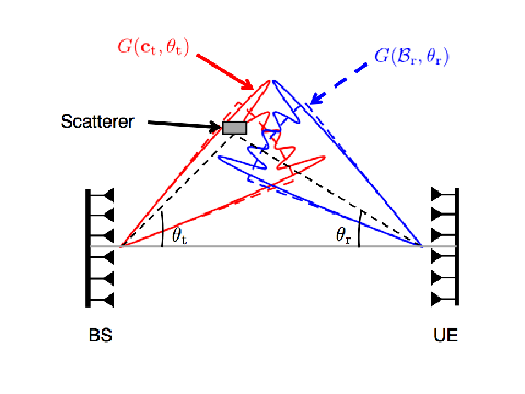
Fig. 1: Actual beam pattern G⁡(𝐜x,θx)G(\mathbf{c}_{\mathrm{x}},\theta_{\mathrm{x}}) generated using the algorithm in [25] with Mt=Mr=128M_{\mathrm{t}}{=}M_{\mathrm{r}}{=}128 antennas. (solid lines) versus sectored model G⁡(ℬx,θx)G(\mathcal{B}_{\mathrm{x}},\theta_{\mathrm{x}}) (dashed lines) [24], on a linear scale. Sidelobes are not visible due to their small magnitude.

II System Model

We consider a downlink scenario in a mm-wave cellular system with one base-station (BS) and one mobile user (UE) at distance dd from the BS, both equipped with uniform linear arrays (ULAs) with MtM_{\mathrm{t}} and MrM_{\mathrm{r}} antennas, respectively, depicted in Fig. 1. Communication occurs over frames of fixed duration TfrT_{\mathrm{fr}}, each composed of NN slots indexed by ℐ≡{0,1,…,N−1}\mathcal{I}{\equiv}\{0,1,\ldots,N{-}1\} of duration T=Tfr/NT{=}T_{\mathrm{fr}}/N, each carrying SS symbols of duration Tsy=T/ST_{\mathrm{sy}}{=}T/S. Let ss be the transmitted symbol, with 𝔼⁡[|s|2]=1\mathbb{E}[|s|^{2}]{=}1. Then, the signal received at the UE is

y=P​𝐜rH​𝐇𝐜t​s+𝐜rH​𝐰,\displaystyle y=\sqrt{P}\mathbf{c}_{\mathrm{r}}^{H}\mathbf{H}\mathbf{c}_{\mathrm{t}}s+\mathbf{c}_{\mathrm{r}}^{H}{\mathbf{w}}, (1)

where PP is the average transmit power of the BS; 𝐇∈ℂMr×Mt\mathbf{H}{\in}\mathbb{C}^{M_{\mathrm{r}}\times M_{\mathrm{t}}} is the channel matrix; 𝐜t∈ℂMt\mathbf{c}_{\mathrm{t}}{\in}\mathbb{C}^{M_{\mathrm{t}}} is the BS beam-forming vector; 𝐜r∈ℂMr\mathbf{c}_{\mathrm{r}}{\in}\mathbb{C}^{M_{\mathrm{r}}} is the UE combining vector; 𝐰∼𝒞​𝒩​(𝟎,N0​Wtot​𝐈){\mathbf{w}}\sim\mathcal{CN}(\boldsymbol{0},N_{0}W_{\mathrm{tot}}\mathbf{I}) is additive white Gaussian noise (AWGN). The symbols N0N_{0} and WtotW_{\mathrm{tot}} denote the one-sided power spectral density of AWGN and the system bandwidth, respectively. By assuming analog beam-forming at both BS and UE, 𝐜t\mathbf{c}_{\mathrm{t}} and 𝐜r\mathbf{c}_{\mathrm{r}} satisfy the unit norm constraints ‖𝐜t‖22=‖𝐜r‖22=1\|\mathbf{c}_{\mathrm{t}}\|_{2}^{2}=\|\mathbf{c}_{\mathrm{r}}\|_{2}^{2}=1. The channel matrix 𝐇\mathbf{H} follows the extended Saleh-Valenzuela geometric model [26],

𝐇=Mt​MrK​∑ℓ=1Khℓ​𝐝r​(θr,ℓ)​𝐝tH​(θt,ℓ),\displaystyle\mathbf{H}=\sqrt{\frac{M_{\mathrm{t}}M_{\mathrm{r}}}{K}}\sum_{\ell=1}^{K}h_{\ell}\;\mathbf{d}_{\mathrm{r}}(\theta_{\mathrm{r},\ell})\mathbf{d}_{\mathrm{t}}^{H}(\theta_{\mathrm{t},\ell}), (2)

where hℓ∈ℂh_{\ell}\in\mathbb{C}, θt,ℓ\theta_{\mathrm{t},\ell} and θr,ℓ\theta_{\mathrm{r},\ell} denote the small scale fading coefficient, AoD and AoA of the ℓt​h\ell^{th} cluster, respectively. The terms 𝐝r​(θr,ℓ)∈ℂMr\mathbf{d}_{\mathrm{r}}(\theta_{\mathrm{r},\ell}){\in}\mathbb{C}^{M_{\mathrm{r}}} and 𝐝t​(θt,ℓ)∈ℂMt\mathbf{d}_{\mathrm{t}}(\theta_{\mathrm{t},\ell}){\in}\mathbb{C}^{M_{\mathrm{t}}} are the UE and BS array response vectors, respectively. For ULAs, θt,ℓ\theta_{\mathrm{t},\ell} (respectively, θr,ℓ\theta_{\mathrm{r},\ell}) is the angle formed between the outgoing (incoming) rays of the llth channel cluster and the perpendicular to the BS (UE) antenna array, as represented in Fig. 1, so that

𝐝x​(θx)=\displaystyle\mathbf{d}_{\mathrm{x}}(\theta_{\mathrm{x}})= 1Mx[1,ej2​π​dxλsinθx,…,ej(Mx−1)2​π​dxλsinθx]⊤,\displaystyle\frac{1}{\sqrt{M_{{\mathrm{x}}}}}\left[1,e^{j\frac{2\pi d_{\mathrm{x}}}{\lambda}\sin\theta_{\mathrm{x}}},\ldots,e^{j(M_{{\mathrm{x}}}-1)\frac{2\pi d_{\mathrm{x}}}{\lambda}\sin\theta_{\mathrm{x}}}\right]^{\top},

where x∈{t,r}\mathrm{x}\in\{{\mathrm{t}},{\mathrm{r}}\}, dtd_{\mathrm{t}} and drd_{\mathrm{r}} are the antenna spacing of the BS and UE arrays, respectively, λ\lambda is the wavelength of the carrier signal. In (2), K≥rank⁡(𝐇)K\geq\mathrm{rank}(\mathbf{H}) is the total number of clusters. Note that 𝐇\mathbf{H} has low-rank if K≪min⁡{Mt,Mr}K\ll\min\{M_{{\mathrm{t}}},M_{{\mathrm{r}}}\}. In this paper, we assume that there is a single dominant cluster (K=1K{=}1). This assumption has been adopted in several previous works (e.g., see [27, 28]), and is motivated by channel measurements and modeling works such as [29], where it is shown that, in dense urban environments, with high probability the mm-wave channel exhibits only one or two clusters, with the dominant one containing most of the signal energy. While our analysis is based on a single cluster model, in Sec. VIII we demonstrate by simulation that the proposed scheme is robust also against multiple clusters. For the single cluster model, we obtain

𝐇=Mt​Mr​h​𝐝r​(θr)​𝐝tH​(θt),\displaystyle\mathbf{H}=\sqrt{M_{\mathrm{t}}M_{\mathrm{r}}}h\;\mathbf{d}_{\mathrm{r}}(\theta_{\mathrm{r}})\mathbf{d}_{\mathrm{t}}^{H}(\theta_{\mathrm{t}}), (3)

where 𝔼⁡[|h|2]=1/ℓ⁡(d)\mathbb{E}[|h|^{2}]=1/\ell(d), ℓ⁡(d)\ell(d) denotes the path loss between BS and UE as a function of distance dd, and 𝜽=(θt,θr)\bm{\theta}=(\theta_{\mathrm{t}},\theta_{\mathrm{r}}) is the single-cluster AoD/AoA pair. We assume that 𝜽\bm{\theta} has prior joint distribution f0​(𝜽)f_{0}(\bm{\theta}) with support supp⁡(f0)=𝒰t,0×𝒰r,0\mathrm{supp}(f_{0}){=}{\mathcal{U}}_{\mathrm{t},0}\times{\mathcal{U}}_{\mathrm{r},0}, which reflects the availability of prior AoD/AoA information acquired from previous beam-alignment phases, or based on geometric constraints (e.g., presence of buildings blocking the signal in certain directions). We assume that hh and 𝜽\bm{\theta} do not change over a frame, whose duration TfrT_{\mathrm{fr}} is chosen based upon the channel and beam coherence times TcT_{c} and TbT_{b} (time duration over which the AoD/AoA do not change appreciably) to satisfy this property. In [30], it has been reported that Tc≪TbT_{c}{\ll}T_{b}. In the numerical values given below, Tb∼100​TcT_{b}{\sim}100T_{c}. Therefore, by choosing Tfr≤TcT_{\mathrm{fr}}{\leq}T_{c}, we ensure that the variations in hh and 𝜽\bm{\theta} over the frame duration TfrT_{\mathrm{fr}} are small and can be ignored. For example, using the relationships of TcT_{c} and TbT_{b} in [30], we obtain Tc≃10T_{c}{\simeq}10[ms] and Tb≃1T_{b}{\simeq}1[s] for a UE velocity of 100[km/h]. In our numerical evaluations, we will therefore use Tfr=10T_{\mathrm{fr}}{=}10[ms]. It is noteworthy that this assumption has also been used extensively in previous beam-alignment works, such as [27, 18, 19].

We assume that blockage occurs at longer time-scales than the frame duration, determined by the geometry of the environment and mobility of users, hence we neglect blockage dynamics within a frame duration [31]. By replacing (3) into (1), and defining the BS and UE beam-forming gains Gx​(𝐜x,θx)=Mx​|𝐝xH​(θx)​𝐜x|2,x∈{t,r}G_{\mathrm{x}}(\mathbf{c}_{\mathrm{x}},\theta_{\mathrm{x}})=M_{\mathrm{x}}|\mathbf{d}_{\mathrm{x}}^{H}(\theta_{\mathrm{x}})\mathbf{c}_{\mathrm{x}}|^{2},\mathrm{x}\in\{\mathrm{t},\mathrm{r}\}, we get

y=h​P​Gt​(𝐜t,θt)⋅Gr​(𝐜r,θr)​ej​Ψ​(𝜽)​s+w^,\displaystyle y=h\sqrt{PG_{\mathrm{t}}(\mathbf{c}_{\mathrm{t}},\theta_{\mathrm{t}})\cdot G_{\mathrm{r}}(\mathbf{c}_{\mathrm{r}},\theta_{\mathrm{r}})}e^{j\Psi(\bm{\theta})}s+\hat{w}, (4)

where w^≜𝐜rH​𝐰∼𝒞​𝒩​(0,N0​Wtot)\hat{w}{\triangleq}\mathbf{c}_{\mathrm{r}}^{H}{\mathbf{w}}\sim\mathcal{CN}(0,N_{0}W_{\mathrm{tot}}) is the noise component and Ψ⁡(𝜽)=∠​𝐝tH​(θt)​𝐜t−∠​𝐝rH​(θr)​𝐜r\Psi(\bm{\theta})=\angle{\mathbf{d}_{\mathrm{t}}^{H}(\theta_{\mathrm{t}})\mathbf{c}_{\mathrm{t}}}-\angle\mathbf{d}_{\mathrm{r}}^{H}(\theta_{\mathrm{r}})\mathbf{c}_{\mathrm{r}} is the phase.

In this paper, we use the sectored antenna model [24] to approximate the BS and UE beam-forming gains, represented in Fig. 1. Under this model,

Gx​(𝐜x,θx)≈Gx​(ℬx,θx)=2​π|ℬx|​χℬx​(θx),x∈{t,r},\displaystyle G_{\mathrm{x}}(\mathbf{c}_{\mathrm{x}},\theta_{\mathrm{x}})\approx G_{\mathrm{x}}(\mathcal{B}_{\mathrm{x}},\theta_{\mathrm{x}})=\frac{2\pi}{|\mathcal{B}_{\mathrm{x}}|}\;\chi_{\mathcal{B}_{\mathrm{x}}}\!\left(\theta_{\mathrm{x}}\right),\quad\mathrm{x}\in\{\mathrm{t},\mathrm{r}\}, (5)

where ℬt⊆(−π,π]\mathcal{B}_{\mathrm{t}}\subseteq(-\pi,\pi] is the range of AoD covered by 𝐜t\mathbf{c}_{\mathrm{t}}, ℬr⊆(−π,π]\mathcal{B}_{\mathrm{r}}\subseteq(-\pi,\pi] is the range of AoA covered by 𝐜r\mathbf{c}_{\mathrm{r}}, χ𝒜​(θ)\chi_{\mathcal{A}}(\theta) is the indicator function of the event θ∈𝒜\theta\in\mathcal{A}, and |𝒜|=∫𝒜𝑑θ|\mathcal{A}|=\int_{\mathcal{A}}\mathrm{d}\theta is the measure of the set 𝒜\mathcal{A}. Hereafter, the two sets ℬt\mathcal{B}_{\mathrm{t}} and ℬr\mathcal{B}_{\mathrm{r}} will be referred to as BS and UE beams, respectively. Additionally, we define ℬk=ℬt,k×ℬr,k\mathcal{B}_{k}=\mathcal{B}_{\mathrm{t},k}\times\mathcal{B}_{\mathrm{r},k} as the 2-dimensional (2D) AoD/AoA support defined by the BS-UE beams. Note that the sectored model is used as an abstraction of the real model, which applies a precoding vector 𝐜t\mathbf{c}_{\mathrm{t}} at the transmitter and a beamforming vector 𝐜r\mathbf{c}_{\mathrm{r}} at the receiver. This abstraction, shown in Fig. 1, is adopted since direct optimization of 𝐜t\mathbf{c}_{\mathrm{t}} and 𝐜r\mathbf{c}_{\mathrm{r}} is not analytically tractable, due to the high dimensionality of the problem. In Sec. VIII we show via Monte-Carlo simulation that, by appropriate design of 𝐜t\mathbf{c}_{\mathrm{t}} and 𝐜r\mathbf{c}_{\mathrm{r}} to approximate the sectored model, our scheme attains near-optimal performance, and outperforms a state-of-the-art bisection search scheme [9]; thus, the sectored antenna model provides a valuable abstraction for practical design. Following the sectored antenna model, we obtain the received signal by replacing Gx​(𝐜x,θx)G_{\mathrm{x}}(\mathbf{c}_{\mathrm{x}},\theta_{\mathrm{x}}) with Gx​(ℬx,θx)G_{\mathrm{x}}(\mathcal{B}_{\mathrm{x}},\theta_{\mathrm{x}}) in (4), yielding

y=h​P​Gt​(ℬt,θt)⋅Gr​(ℬr,θr)​ej​Ψ​(𝜽)​s+w^.\displaystyle y=h\sqrt{PG_{\mathrm{t}}(\mathcal{B}_{\mathrm{t}},\theta_{\mathrm{t}})\cdot G_{\mathrm{r}}(\mathcal{B}_{\mathrm{r}},\theta_{\mathrm{r}})}e^{j\Psi(\bm{\theta})}s+\hat{w}. (6)

Although the analysis in this paper is presented for ULAs (2D beamforming), the proposed scheme can be extended to the case of uniform planar arrays with 3D beamforming, by interpreting θx,x∈{t,r}\theta_{\mathrm{x}},\mathrm{x}\in\{\mathrm{t},\mathrm{r}\} as a vector denoting the azimuth and elevation pair in (−π,π]2(-\pi,\pi]^{2} and the beam ℬx⊆(π,π]2\mathcal{B}_{\mathrm{x}}\subseteq(\pi,\pi]^{2}. For notational convenience and ease of exposition, in this paper we focus on the 2D beamforming case (also adopted in, e.g., [22, 9, 18, 23]).

The entire frame duration is split into two, possibly interleaved phases: a beam-alignment phase, whose goal is to detect the best beam to be used in the data communication phase. To this end, we partition the slots ℐ\mathcal{I} in each frame into the indices in the set ℐs\mathcal{I}_{s}, reserved for beam-alignment, and those in the set ℐd\mathcal{I}_{d}, reserved for data communication, where ℐs∩ℐd=∅\mathcal{I}_{s}{\cap}\mathcal{I}_{d}{=}\emptyset and ℐs∪ℐd=ℐ\mathcal{I}_{s}{\cup}\mathcal{I}_{d}{=}\mathcal{I}. The optimal frame partition and duration of beam-alignment are part of our design. In the sequel, we describe the operations performed in the beam-alignment and data communication slots, and characterize their energy consumption.

Beam-Alignment: At the beginning of each slot k∈ℐsk{\in}\mathcal{I}_{s}, the BS sends a beacon signal 𝐬\mathbf{s} of duration TB<TT_{B}{<}T using the transmit beam ℬt,k\mathcal{B}_{\mathrm{t},k} with power PkP_{k},11 1 In practice, there are limits on how small the beacon duration can be made, due to peak power constraints [32], beacon synchronization errors [4], and auto-correlation properties of the beacon sequence [4]. and the UE receives the signal using the receive beam ℬr,k\mathcal{B}_{\mathrm{r},k}. Note that ℬk=ℬt,k×ℬr,k\mathcal{B}_{k}{=}\mathcal{B}_{\mathrm{t},k}{\times}\mathcal{B}_{\mathrm{r},k} and PkP_{k} are design parameters. If the UE detects the beacon (i.e., the AoD/AoA 𝜽\bm{\theta} is in ℬk\mathcal{B}_{k}, or a false-alarm occurs, see [33]), then, in the remaining portion of the slot of duration T−TBT{-}T_{B}, it transmits an acknowledgment (ACK\mathrm{ACK}) packet to the BS, denoted as Ck=ACKC_{k}{=}\mathrm{ACK}. Otherwise (the UE does not detect the beacon due to either mis-alignment or misdetection error), it transmits Ck=NACKC_{k}{=}\mathrm{NACK}. We assume that the ACK/NACK\mathrm{ACK}/\mathrm{NACK} signal CkC_{k} is received perfectly and within the end of the slot by the BS (for instance, by using a conventional microwave technology as a control channel [34]).

As a result of (6), the UE attempts to detect the beam, and generates the ACK/NACK signal based on the following hypothesis testing problem,

ℋ1:\displaystyle\hskip-7.11317pt\mathcal{H}_{1}:\; 𝐲k=N0​Wtot​νk​h​ej​Ψk​(𝜽)​𝐬+𝐰^k,\displaystyle\mathbf{y}_{k}{=}\sqrt{N_{0}W_{\mathrm{tot}}\nu_{k}}he^{j\Psi_{k}(\bm{\theta})}\mathbf{s}{+}\hat{\mathbf{w}}_{k},\hskip-25.60747pt (alignment, 𝜽∈ℬk\bm{\theta}{\in}\mathcal{B}_{k}) (7)
ℋ0:\displaystyle\hskip-7.11317pt\mathcal{H}_{0}:\; 𝐲k=𝐰^k,\displaystyle\mathbf{y}_{k}{=}\hat{\mathbf{w}}_{k},\hskip-28.45274pt (misalignment, 𝜽∉ℬk\bm{\theta}{\notin}\mathcal{B}_{k}) (8)

where 𝐲k\mathbf{y}_{k} is the received signal vector, 𝐬\mathbf{s} is the transmitted symbol sequence, 𝐰^k∼𝒞​𝒩​(𝟎,N0​Wtot​𝐈)\hat{\mathbf{w}}_{k}{\sim}\mathcal{CN}(\boldsymbol{0},N_{0}W_{\mathrm{tot}}\mathbf{I}) is the AWGN vector, and νk\nu_{k} is related to the beam-forming gain in slot kk,

νk=(2​π)2​PkN0​Wtot​|ℬk|.\displaystyle\nu_{k}=\frac{(2\pi)^{2}P_{k}}{N_{0}W_{\mathrm{tot}}|\mathcal{B}_{k}|}. (9)

The optimal detector depends on the availability of prior information on hh. We assume that an estimate of the channel gain γ=|h|2\gamma{=}|h|^{2} is available at the BS and UE at the beginning of each frame, denoted as γ^=|h^|2\hat{\gamma}{=}|\hat{h}|^{2}, where h^=h+e\hat{h}{=}h+e and e∼𝒞​𝒩​(0,σe2)e{\sim}\mathcal{CN}(0,\sigma_{\mathrm{e}}^{2}) denotes the estimation noise. A Neyman-Pearson threshold detector is optimal in this case,

|𝐬H​𝐲k|2N0​Wtot​‖𝐬‖22​≶ℋ1ℋ0τth.\displaystyle\frac{|\mathbf{s}^{H}\mathbf{y}_{k}|^{2}}{N_{0}W_{\mathrm{tot}}\|\mathbf{s}\|_{2}^{2}}\mathop{\lessgtr}_{\mathcal{H}_{1}}^{\mathcal{H}_{0}}\tau_{\mathrm{th}}. (10)

The detector’s threshold τth\tau_{\mathrm{th}} and the transmission power PkP_{k} are designed based on the channel gain estimate γ^\hat{\gamma}, so as to satisfy constraints on the false-alarm and misdetection probabilities, pfa,pmd≤pep_{\mathrm{fa}},p_{\mathrm{md}}\leq p_{e}. We now compute these probabilities under the simplifying assumption that h^\hat{h} and ee are independent, so that h|h^∼𝒞​𝒩​(h^,σe2)h|\hat{h}\sim\mathcal{CN}(\hat{h},\sigma_{\mathrm{e}}^{2}). Let zk≜𝐬H​𝐲kN0​Wtot​‖𝐬‖2z_{k}\triangleq\frac{\mathbf{s}^{H}\mathbf{y}_{k}}{\sqrt{N_{0}W_{\mathrm{tot}}}\|\mathbf{s}\|_{2}}, so that |zk|2|z_{k}|^{2} is the decision variable. We observe that

zk={νk​h​ej​Ψk​(𝜽)​‖𝐬‖2+𝐬H​𝐰^kN0​Wtot​‖𝐬‖2, if ℋ1 is true;𝐬H​𝐰^kN0​Wtot​‖𝐬‖2, if ℋ0 is true.\displaystyle z_{k}=\begin{cases}\sqrt{\nu_{k}}he^{j\Psi_{k}(\bm{\theta})}\|\mathbf{s}\|_{2}+\frac{\mathbf{s}^{H}\hat{\mathbf{w}}_{k}}{\sqrt{N_{0}W_{\mathrm{tot}}}\|\mathbf{s}\|_{2}},&\text{ if $\mathcal{H}_{1}$ is true;}\\ \frac{\mathbf{s}^{H}\hat{\mathbf{w}}_{k}}{\sqrt{N_{0}W_{\mathrm{tot}}}\|\mathbf{s}\|_{2}},&\text{ if $\mathcal{H}_{0}$ is true.}\end{cases}

Since h^\hat{h} and 𝐰^k\hat{\mathbf{w}}_{k} are independent and h=h^−eh=\hat{h}-e, we obtain

f⁡(zk|h^,ℋ1,𝜽)=𝒞​𝒩​(νk​h^​ej​Ψk​(𝜽)​‖𝐬‖2,1+νk​‖𝐬‖22​σe2),\displaystyle\!f(z_{k}|\hat{h},\mathcal{H}_{1},\bm{\theta})\!=\mathcal{CN}\!\left(\!\sqrt{\nu_{k}}\hat{h}e^{j\Psi_{k}(\bm{\theta})}\|\mathbf{s}\|_{2},1{+}{\nu_{k}}{\|\mathbf{s}\|_{2}^{2}}\sigma_{\mathrm{e}}^{2}\right)\!,\!\! (11)
f⁡(zk|h^,ℋ0)=𝒞​𝒩​(0,1),\displaystyle f(z_{k}|\hat{h},\mathcal{H}_{0})=\mathcal{CN}\left(0,1\right), (12)

so that [|zk|2|h^,ℋ0]∼Exponential(1)[|z_{k}|^{2}|\hat{h},\mathcal{H}_{0}]\sim\mathrm{Exponential}(1), and the false-alarm probability can be expressed as

pfa​(τth)≜ℙ⁡(|zk|2>τth|h^,ℋ0)=exp⁡(−τth).\displaystyle p_{\mathrm{fa}}(\tau_{\mathrm{th}})\triangleq\mathbb{P}\left(|z_{k}|^{2}>\tau_{\mathrm{th}}\big|\hat{h},\mathcal{H}_{0}\right)=\exp\left(-\tau_{\mathrm{th}}\right). (13)

Similarly, the misdetection probability is found to be

pmd​(νk,τth,γ^)≜ℙ⁡(|zk|2<τth|h^,ℋ1)\displaystyle p_{\mathrm{md}}(\nu_{k},\tau_{\mathrm{th}},\hat{\gamma})\triangleq\mathbb{P}\left(|z_{k}|^{2}<\tau_{\mathrm{th}}\big|\hat{h},\mathcal{H}_{1}\right) =1−Q1​(2​γ^​νk​‖𝐬‖221+νk​‖𝐬‖22​σe2,2​τth1+νk​‖𝐬‖22​σe2),\displaystyle=1-Q_{1}\left(\sqrt{\frac{2\hat{\gamma}\nu_{k}\|\mathbf{s}\|_{2}^{2}}{1+\nu_{k}\|\mathbf{s}\|_{2}^{2}\sigma_{\mathrm{e}}^{2}}},\sqrt{\frac{2\tau_{\mathrm{th}}}{1+\nu_{k}\|\mathbf{s}\|_{2}^{2}\sigma_{\mathrm{e}}^{2}}}\right), (14)

where Q1​(⋅)Q_{1}(\cdot) is the first-order Marcum’s Q function [35]. In fact, zk|(h^,ℋ1)z_{k}|(\hat{h},\mathcal{H}_{1}) is complex Gaussian as in (11), so that, given (γ^,ℋ1)(\hat{\gamma},\mathcal{H}_{1}), 2​|zk|21+νk​‖𝐬‖22​σe2\frac{2|z_{k}|^{2}}{{1+\nu_{k}\|\mathbf{s}\|_{2}^{2}\sigma_{\mathrm{e}}^{2}}} follows non-central chi-square distribution with 2 degrees of freedom and non-centrality parameter 2​νk​γ^​‖𝐬‖221+νk​‖𝐬‖22​σe2\frac{2\nu_{k}\hat{\gamma}\|\mathbf{s}\|_{2}^{2}}{1+{\nu_{k}}{\|\mathbf{s}\|_{2}^{2}}\sigma_{\mathrm{e}}^{2}}.

Herein, we design τth\tau_{\mathrm{th}} and PkP_{k} to achieve pfa,pmd≤pep_{\mathrm{fa}},p_{\mathrm{md}}\leq p_{\mathrm{e}}. To satisfy pfa​(τth)≤pep_{\mathrm{fa}}(\tau_{\mathrm{th}})\leq p_{\mathrm{e}} we need

τth≥−ln⁡(pe).\displaystyle\tau_{\mathrm{th}}\geq-\ln\left(p_{\mathrm{e}}\right). (15)

Since Q1​(a,b)Q_{1}(a,b) is an increasing function of a≥0a{\geq}0 and a decreasing function of b≥0b{\geq}0, it follows that pmd​(νk,τth)p_{\mathrm{md}}(\nu_{k},\tau_{\mathrm{th}}) is a decreasing function of νk≥0\nu_{k}{\geq}0 and an increasing function of τth≥0\tau_{\mathrm{th}}{\geq}0. Then, to guarantee pmd​(νk,τth,γ^)≤pep_{\mathrm{md}}(\nu_{k},\tau_{\mathrm{th}},\hat{\gamma}){\leq}p_{\mathrm{e}}, (15) should be satisfied with equality to attain the smallest pmdp_{\mathrm{md}}; additionally, there exists ν∗>0\nu^{*}{>}0, determined as the unique solution of pmd​(ν∗,τth,γ^)=pep_{\mathrm{md}}(\nu^{*},\tau_{\mathrm{th}},\hat{\gamma}){=}p_{\mathrm{e}} and independent of the beam shape ℬk\mathcal{B}_{k}, such that pmd​(νk,τth,γ^)≤pep_{\mathrm{md}}(\nu_{k},\tau_{\mathrm{th}},\hat{\gamma}){\leq}p_{\mathrm{e}} iff (if and only if) νk≥ν∗\nu_{k}{\geq}\nu^{*}. Then, using (9) and letting Ek≜Pk​Tsy​‖𝐬‖22E_{k}{\triangleq}P_{k}T_{\mathrm{sy}}\|\mathbf{s}\|_{2}^{2} be the energy incurred for the transmission of the beacon 𝐬\mathbf{s} in slot kk, EkE_{k} should satisfy

Ek≥ϕs​(pe)​|ℬk|,\displaystyle E_{k}\geq\phi_{s}(p_{\mathrm{e}})|\mathcal{B}_{k}|, (16)
where ​ϕs​(pe)≜N0​Wtot​ν∗​Tsy​‖𝐬‖22/(2​π)2\displaystyle\text{where }\phi_{s}(p_{\mathrm{e}}){\triangleq}N_{0}W_{\mathrm{tot}}\nu^{*}T_{\mathrm{sy}}\|\mathbf{s}\|_{2}^{2}/(2\pi)^{2} (17)

is the energy/rad2\text{energy}/\text{rad}^{2} required to achieve false-alarm and misdetection probabilities equal to pep_{\mathrm{e}}.

Note that false-alarm and misdetection errors are deleterious to performance, since they result in mis-alignment and outages during data transmission. Therefore, they should be minimized. For this reason, in the first part of this paper we assume that pe≪1p_{\mathrm{e}}{\ll}1, and neglect the impact of these errors on beam-alignment. Thus, we let Ek≥ϕs​|ℬk|E_{k}{\geq}\phi_{s}|\mathcal{B}_{k}| be the energy required in each beam-alignment slot to guarantee detection with high probability, where ϕs\phi_{s} is computed under some small pe≪1p_{\mathrm{e}}\ll 1. We will consider the impact of these errors in Sec. VII.22 2 The design of beam-alignment schemes robust to errors when pe≪̸1p_{\mathrm{e}}\not\ll 1 has been considered in [36]. Its analysis is outside the scope of this paper.

Data Communication: In the communication slots indexed by k∈ℐd{k\in}\mathcal{I}_{d}, the BS uses ℬt,k\mathcal{B}_{\mathrm{t},k}, rate RkR_{k}, and transmit power PkP_{k}, while the UE processes the received signal using the beam ℬr,k\mathcal{B}_{\mathrm{r},k}. Therefore, letting γ=|h|2\gamma=|h|^{2} and νk\nu_{k} as in (9). the instantaneous SNR can be expressed as

𝖲𝖭𝖱k\displaystyle{\mathsf{SNR}}_{k} =γ​Pk​Gt​(ℬt,k,θt)​Gr​(ℬr,k,θr)N0​Wtot\displaystyle=\frac{\gamma P_{k}G_{\mathrm{t}}(\mathcal{B}_{\mathrm{t},k},\theta_{\mathrm{t}})G_{\mathrm{r}}(\mathcal{B}_{\mathrm{r},k},\theta_{\mathrm{r}})}{N_{0}W_{\mathrm{tot}}}
=νk​γ​χℬt,k​(θt)​χℬr,k​(θr).\displaystyle=\nu_{k}\gamma\chi_{\mathcal{B}_{\mathrm{t},k}}(\theta_{\mathrm{t}})\chi_{\mathcal{B}_{\mathrm{r},k}}(\theta_{\mathrm{r}}). (18)

Outage occurs if Wtot​log2⁡(1+𝖲𝖭𝖱k)<RkW_{\mathrm{tot}}\log_{2}(1{+}\mathsf{SNR}_{k}){<}R_{k} due to either mis-alignment between transmitter and receiver, or low channel gain γ\gamma. The probability of this event, po​u​tp_{out}, can be inferred from the posterior probability distribution of the AoD/AoA pair 𝜽\bm{\theta} and the channel gain γ\gamma, given its estimate γ^\hat{\gamma}, and the history of BS-UE beams and feedback until slot kk, denoted as ℋk≜{(ℬ0,C0),…,(ℬk−1,Ck−1)}\mathcal{H}^{k}\triangleq\{(\mathcal{B}_{0},C_{0}),\ldots,(\mathcal{B}_{k-1},C_{k-1})\}. Thus, po​u​t≜ℙ⁡(Wtot​log2⁡(1+𝖲𝖭𝖱k)<Rk|γ^,ℋk)p_{out}\triangleq\mathbb{P}(W_{\mathrm{tot}}\log_{2}(1+{\mathsf{SNR}}_{k})<R_{k}|\hat{\gamma},\mathcal{H}^{k}), yielding

po​u​t\displaystyle p_{out} =(a)ℙ⁡(𝖲𝖭𝖱k<2RkWtot−1|γ^,𝜽∈ℬk)​ℙ​(𝜽∈ℬk|ℋk)\displaystyle\stackrel{{\scriptstyle(a)}}{{=}}\mathbb{P}\left({\mathsf{SNR}}_{k}<2^{\frac{R_{k}}{W_{\mathrm{tot}}}}-1|\hat{\gamma},\bm{\theta}\in\mathcal{B}_{k}\right)\mathbb{P}(\bm{\theta}\in\mathcal{B}_{k}|\mathcal{H}^{k})
+ℙ⁡(𝜽∉ℬk|ℋk)\displaystyle\qquad+\mathbb{P}(\bm{\theta}\not\in\mathcal{B}_{k}|\mathcal{H}^{k})
=(b)1−F¯γ​(2RkWtot−1νk|γ^)​ℙ​(𝜽∈ℬk|ℋk),\displaystyle\stackrel{{\scriptstyle(b)}}{{=}}1-\bar{F}_{\gamma}\left(\frac{2^{\frac{R_{k}}{W_{\mathrm{tot}}}}-1}{\nu_{k}}\bigg|\hat{\gamma}\right)\mathbb{P}(\bm{\theta}\in\mathcal{B}_{k}|\mathcal{H}^{k}), (19)

where (a) follows from the law of total probability and ℙ⁡(𝜽∈ℬk|ℋk)\mathbb{P}(\bm{\theta}{\in}\mathcal{B}_{k}|\mathcal{H}^{k}) denotes the probability of correct beam-alignment; (b) follows by substituting F¯γ​(x|γ^)≜ℙ⁡(γ≥x|γ^)\bar{F}_{\gamma}(x|\hat{\gamma}){\triangleq}\mathbb{P}(\gamma{\geq}x|\hat{\gamma}) into (a), given as

F¯γ​(x|γ^)=Q1​(2​γ^/σe2,2​x/σe2).\displaystyle\bar{F}_{\gamma}(x|\hat{\gamma})=Q_{1}\left(\sqrt{{2\hat{\gamma}}/{\sigma_{e}^{2}}},\sqrt{{2x}/{\sigma_{e}^{2}}}\right). (20)

Herein, we use the notion of ϵ\epsilon-outage capacity to design RkR_{k}, defined as the largest transmission rate such that po​u​t≤ϵp_{out}{\leq}\epsilon, for a target outage probability ϵ<1\epsilon{<}1. This can be expressed as

𝒞ϵ(Pk,ℬk|ℋk,γ^)≜Wtotlog2(1+νkF¯γ−1(1−ϵℙ⁡(𝜽∈ℬk|ℋk)|γ^)),\displaystyle{\mathcal{C}_{\epsilon}(P_{k},\mathcal{B}_{k}|\mathcal{H}^{k},\hat{\gamma})}\triangleq W_{\mathrm{tot}}\log_{2}\left(1+\nu_{k}\bar{F}_{\gamma}^{-1}\left(\left.\frac{1-\epsilon}{\mathbb{P}(\bm{\theta}{\in}\mathcal{B}_{k}|\mathcal{H}^{k})}\right|\hat{\gamma}\right)\right), (21)

where F¯γ−1(⋅|γ^)\bar{F}_{\gamma}^{-1}(\cdot|\hat{\gamma}) denotes the inverse posterior CCDF of γ\gamma, conditional on γ^\hat{\gamma}. In other words, if Rk≤𝒞ϵ(Pk,ℬk|ℋk,γ^)R_{k}{\leq}{\mathcal{C}_{\epsilon}(P_{k},\mathcal{B}_{k}|\mathcal{H}^{k},\hat{\gamma})}, then the transmission is successful with probability at least 1−ϵ1{-}\epsilon, and the average rate is at least (1−ϵ)​Rk(1{-}\epsilon)R_{k}. Note that, in order to achieve the target po​u​t≤ϵp_{out}{\leq}\epsilon, the probability of correct beam-alignment must satisfy ℙ⁡(𝜽∈ℬk|ℋk)≥1−ϵ\mathbb{P}(\bm{\theta}{\in}\mathcal{B}_{k}|\mathcal{H}^{k}){\geq}1{-}\epsilon. This can be achieved with a proper choice of ℬk\mathcal{B}_{k}, as discussed next.

Since the ACK/NACK feedback after data communication is generated by higher layers (e.g., network or transport layer), we do not use it to improve beam-alignment. We define Ck=NULLC_{k}{=}\mathrm{NULL}, ∀k∈ℐd\forall k{\in}\mathcal{I}_{d}, to distinguish it from the ACK/NACK feedback signal in the beam-alignment slots.

III Problem Formulation

In this section, we formulate the optimization problem, and characterize it as a Markov decision process (MDP). The goal is to minimize the power consumption at the BS over a frame duration, while achieving the quality of service (QoS) requirements of the UE (rate and delay). Therefore, the objective function of the following optimization problem captures the beam-alignment and data communication energy costs; the QoS requirements are specified in the constraints through a rate requirement RminR_{\min} of the UE along with an outage probability of ϵ\epsilon; additionally, the frame duration TfrT_{\mathrm{fr}} represents a delay guarantee on data transmission. The design variables in slot kk are denoted by the 4-tuple 𝐚k=(ξk,Pk,ℬk,Rk){\mathbf{a}}_{k}=(\xi_{k},P_{k},\mathcal{B}_{k},R_{k}), where ξk\xi_{k} corresponds to the decision of whether to perform beam-alignment (ξk=1\xi_{k}{=}1) or data communication (ξk=0\xi_{k}{=}0); we let Rk=0R_{k}{=}0 for beam-alignment slots (ξk=1\xi_{k}=1). With this choice of 𝐚k\mathbf{a}_{k}, we aim to optimally select the beam-alignment slots ℐs\mathcal{I}_{s} and data communication slots ℐd\mathcal{I}_{d}. If a slots is selected for beam-alignment (ξk=1\xi_{k}=1), we aim to optimize the associated power PkP_{k} and 2D beam ℬk\mathcal{B}_{k}. Likewise, if a slot is selected for data communication (ξk=0\xi_{k}=0), we aim to optimize the associated power PkP_{k}, data rate RkR_{k}, and 2D beam ℬk\mathcal{B}_{k}. Mathematically, the optimization problem is stated as

P1:\displaystyle\mathrm{P}_{1}: P¯≜min𝐚0,…,𝐚N−11Tfr​𝔼​[∑k=0N−1Ek|f0]\displaystyle\quad\bar{P}\triangleq\min_{\mathbf{a}_{0},\ldots,\mathbf{a}_{N-1}}\quad\frac{1}{T_{\mathrm{fr}}}\mathbb{E}\left[\sum_{k=0}^{N-1}E_{k}\bigg|f_{0}\right] (22)
s.t. 𝐚k=(ξk,Pk,ℬk,Rk),∀k,\displaystyle{\mathbf{a}}_{k}{=}(\xi_{k},P_{k},\mathcal{B}_{k},R_{k}),\forall k,
ℬk=ℬt,k×ℬr,k⊆[−π,π]2,∀k,\displaystyle\mathcal{B}_{k}{=}\mathcal{B}_{\mathrm{t},k}{\times}\mathcal{B}_{\mathrm{r},k}\subseteq[-\pi,\pi]^{2},\forall k, (23)
Ek≥ϕs​|ℬk|,∀k∈ℐs,\displaystyle E_{k}\geq\phi_{s}|\mathcal{B}_{k}|,\ \forall k\in\mathcal{I}_{s}, (24)
1N∑kRk≥Rmin,Rk≤𝒞ϵ(Pk,ℬk|ℋk,γ^),∀k∈ℐd,\displaystyle\frac{1}{N}\sum_{k}R_{k}{\geq}R_{\min},\ R_{k}{\leq}\mathcal{C}_{\epsilon}(P_{k},\mathcal{B}_{k}|\mathcal{H}^{k},\hat{\gamma}),\forall k{\in}\mathcal{I}_{d}, (25)
Pk=Ek/[ξk​TB+(1−ξk)​T],∀k,\displaystyle P_{k}=E_{k}/[\xi_{k}T_{B}+(1-\xi_{k})T],\ \forall k, (26)

where f0f_{0} in (22) denotes the prior belief over 𝜽\bm{\theta}; (23) defines the 2D beam ℬk\mathcal{B}_{k}; (24) gives the energy consumption in the beam-alignment slots; (25) ensures the rate requirement RminR_{\min} over the frame, and that RkR_{k} is within the ϵ\epsilon-outage capacity, see (21); (26) gives the relation between energy and power.33 3 Data communication takes the entire slot, whereas beam-alignment occurs over a portion TB<TT_{B}<T of the slot to allow for the time to receive the ACK/NACK feedback from the receiver. Since the cost is the average BS power consumption, the inequality constraints (24)-(25) must be tight, i.e., we replace them with

Ek=ξk​ϕs​|ℬk|+(1−ξk)​ψd​(Rk)​|ℬk|F¯γ−1​(1−ϵℙ⁡(𝜽∈ℬk|ℋk)|γ^),\displaystyle E_{k}=\xi_{k}\phi_{s}|\mathcal{B}_{k}|+(1-\xi_{k})\frac{{\psi}_{d}(R_{k})|\mathcal{B}_{k}|}{\bar{F}_{\gamma}^{-1}\left(\frac{1-\epsilon}{\mathbb{P}(\bm{\theta}\in\mathcal{B}_{k}|\mathcal{H}^{k})}\big|\hat{\gamma}\right)}, (27)
1N​∑kRk=Rmin,\displaystyle\frac{1}{N}\sum_{k}R_{k}=R_{\min}, (28)

where (27) when ξk=0\xi_{k}{=}0 is obtained by inverting (25) via (21) and (9) (with equality) to find PkP_{k} and Ek=Pk​TE_{k}=P_{k}T, and we have defined the energy/rad2\text{energy}/\text{rad}^{2} required to achieve the rate RR

ψd​(R)≜(2​π)−2​N0​Wtot​T​(2RWtot−1).{\psi}_{d}(R)\triangleq(2\pi)^{-2}N_{0}W_{\mathrm{tot}}T(2^{\frac{R}{W_{\mathrm{tot}}}}-1).

Hereafter, we exclude PkP_{k} from the design space, since it is uniquely defined by the set of equality constraints (26)-(27). Thus, we simplify the design variable to 𝐚k=(ξk,ℬk,Rk){\mathbf{a}}_{k}=(\xi_{k},\mathcal{B}_{k},R_{k}).

We pose P1\mathrm{P}_{1} as an MDP [37] over the time horizon ℐ\mathcal{I}. The state at the start of slot kk is (fk,Dk)(f_{k},D_{k}), where fkf_{k} is the probability distribution over the AoD/AoA pair 𝜽\bm{\theta}, given the history ℋk\mathcal{H}^{k} up to slot kk, denoted as belief; DkD_{k} is the backlog (untransmitted data bits). Initially, f0f_{0} is the prior belief and D0≜Rmin​TfrD_{0}{\triangleq}R_{\min}T_{\mathrm{fr}}. Given (fk,Dk)(f_{k},D_{k}), the BS and UE select 𝐚k=(ξk,ℬk,Rk)\mathbf{a}_{k}{=}\left(\xi_{k},\mathcal{B}_{k},R_{k}\right).44 4 Since feedback is error-free, both BS and UE have the same information to generate the action 𝐚k\mathbf{a}_{k} and their beams. Then, the UE generates the feedback signal: if ξk=0\xi_{k}{=}0 (data communication), then Ck=NULLC_{k}{=}\mathrm{NULL}; if ξk=1\xi_{k}{=}1 (beam-alignment), then Ck=ACKC_{k}{=}\mathrm{ACK} if 𝜽∈ℬk\bm{\theta}{\in}\mathcal{B}_{k}, with probability

ℙ⁡(Ck=ACK|fk,𝐚k)=∫ℬkfk​(𝜽)​𝑑𝜽,\displaystyle\mathbb{P}(C_{k}=\mathrm{ACK}|f_{k},\mathbf{a}_{k})=\int_{\mathcal{B}_{k}}f_{k}(\bm{\theta})d\bm{\theta}, (29)

and Ck=NACKC_{k}{=}\mathrm{NACK} otherwise. Upon receiving CkC_{k}, the new backlog in slot k+1k+1 becomes55 5 If Dk+1≤0D_{k+1}\leq 0, all bits have been transmitted.

Dk+1=max{Dk−RkT,0},\displaystyle D_{k+1}=\max\bigr\{D_{k}-R_{k}T,0\bigr\}, (30)

and the new belief fk+1f_{k+1} is computed via Bayes’ rule, as given in the following lemma.

Lemma 1.

Let f0f_{0} be the prior belief on 𝛉\bm{\theta} with support supp⁡(f0)=𝒰0\mathrm{supp}(f_{0})={\mathcal{U}}_{0}. Then,

fk​(𝜽)=f0​(𝜽)∫𝒰kf0​(𝜽~)​𝑑𝜽~​χ𝒰k​(𝜽),\displaystyle f_{k}(\bm{\theta})=\frac{f_{0}(\bm{\theta})}{\int_{{\mathcal{U}}_{k}}f_{0}(\tilde{\bm{\theta}})\mathrm{d}\tilde{\bm{\theta}}}\chi_{{\mathcal{U}}_{k}}(\bm{\theta}), (31)

where 𝒰k≜supp⁡(fk){\mathcal{U}}_{k}\triangleq\mathrm{supp}(f_{k}) is updated recursively as

𝒰k+1={𝒰k∩ℬk,k∈ℐs,Ck=ACK𝒰k∖ℬk,k∈ℐs,Ck=NACK𝒰k,k∈ℐd.\displaystyle{\mathcal{U}}_{k+1}=\left\{\begin{array}[]{ll}{\mathcal{U}}_{k}\cap\mathcal{B}_{k},&k\in\mathcal{I}_{\mathrm{s}},C_{k}=\mathrm{ACK}\\ {\mathcal{U}}_{k}\setminus{\mathcal{B}_{k}},&k\in\mathcal{I}_{\mathrm{s}},C_{k}=\mathrm{NACK}\\ {\mathcal{U}}_{k},&k\in\mathcal{I}_{\mathrm{d}}.\end{array}\right.
Proof.

The proof follows by induction using Bayes’ rule. In fact, if Ck=ACKC_{k}{=}\mathrm{ACK} in a beam-alignment slot, then it can be inferred that 𝜽∈𝒰k∩ℬk\bm{\theta}{\in}\mathcal{U}_{k}{\cap}\mathcal{B}_{k}; otherwise (Ck=NACKC_{k}{=}\mathrm{NACK}) the UE lies outside ℬk\mathcal{B}_{k}, but within the support of fkf_{k}, i.e., 𝜽∈𝒰k∖ℬk\bm{\theta}{\in}\mathcal{U}_{k}{\setminus}\mathcal{B}_{k}. In the data communication slots, no feedback is generated, hence fk+1=fkf_{k+1}{=}f_{k} and 𝒰k+1=𝒰k{\mathcal{U}}_{k+1}{=}{\mathcal{U}}_{k}. A detailed proof is given in Appendix A. ∎

Lemma 1 implies that 𝒰k\mathcal{U}_{k} is a sufficient statistic for decision making in slot kk, and is updated recursively via (1). Accordingly, the state space is defined as

𝒮≡{(𝒰,D):𝒰⊆𝒰0,0≤D≤D0}.\displaystyle\mathcal{S}\equiv\{(\mathcal{U},D):\mathcal{U}\subseteq\mathcal{U}_{0},0\leq D\leq D_{0}\}. (35)

Given the data backlog Dk=DD_{k}{=}D, the action space is expressed as66 6 Note that, for a data communication action (0,ℬ,R)(0,\mathcal{B},R), we assume that R>0R>0; in fact, data communication with zero rate is equivalent to a beam-alignment action (1,∅,0)(1,\emptyset,0) with empty beam.

𝒜⁡(D)≡\displaystyle\mathcal{A}(D)\equiv {(0,ℬ,R):ℬ≡ℬt×ℬr⊆[−π,π]2,0<R≤D/T}\displaystyle\left\{(0,\mathcal{B},R):\mathcal{B}\equiv\mathcal{B}_{\mathrm{t}}\times\mathcal{B}_{\mathrm{r}}\subseteq[-\pi,\pi]^{2},0{<}R{\leq}D/T\right\}
∪{(1,ℬ,0):ℬ≡ℬt×ℬr⊆[−π,π]2}.\displaystyle\cup\left\{(1,\mathcal{B},0):\mathcal{B}\equiv\mathcal{B}_{\mathrm{t}}\times\mathcal{B}_{\mathrm{r}}\subseteq[-\pi,\pi]^{2}\right\}. (36)

Given (𝒰k,Dk)∈𝒮({\mathcal{U}}_{k},D_{k})\in\mathcal{S}, the action 𝐚k∈𝒜⁡(Dk)\mathbf{a}_{k}{\in}\mathcal{A}(D_{k}) is chosen based on policy μk\mu_{k}, which determines the BS-UE beam ℬk\mathcal{B}_{k} and whether to perform beam-alignment (ξk=1\xi_{k}{=}1, Rk=0R_{k}{=}0) or data communication (ξk=0\xi_{k}{=}0, Rk>0R_{k}{>}0), with energy cost EkE_{k} given by (27). With this notation, we can express the problem P1\mathrm{P}_{1} as that of finding the policy μ∗\mu^{*} which minimizes the power consumption under rate requirement and outage probability constraints,

P2:P¯≜minμ1Tfr𝔼μ[∑k=0N−1c(𝐚k;𝒰k,Dk)|𝒰0,D0,f0],\displaystyle\mathrm{P}_{2}:\quad\bar{P}\triangleq\min_{\mu}\;\frac{1}{T_{\mathrm{fr}}}\mathbb{E}_{\mu}\Biggl[\sum_{k=0}^{N-1}c(\mathbf{a}_{k};{\mathcal{U}}_{k},D_{k})\bigg|{\mathcal{U}}_{0},D_{0},f_{0}\Biggr],
s.t.Dk+1=Dk−T​Rk,∀k∈ℐ,DN=0,\displaystyle\mathrm{s.t.}\qquad D_{k+1}=D_{k}-TR_{k},\forall k\in\mathcal{I},\;\;D_{N}=0, (37)

where we have defined the cost per stage in state (𝒰k,Dk)({\mathcal{U}}_{k},D_{k}) under action 𝐚k\mathbf{a}_{k} as

c⁡(𝐚k,𝒰k,Dk)=[ξk​ϕs+(1−ξk)​ψd​(Rk)F¯γ−1​(1−ϵℙ⁡(𝜽∈ℬk|𝒰k)|γ^)]​|ℬk|,\displaystyle c(\mathbf{a}_{k};{\mathcal{U}}_{k},D_{k}){=}\left[\xi_{k}\phi_{s}{+}\frac{(1{-}\xi_{k})\psi_{d}(R_{k})}{\bar{F}_{\gamma}^{-1}\left(\frac{1-\epsilon}{\mathbb{P}(\bm{\theta}\in\mathcal{B}_{k}|\mathcal{U}_{k})}\big|\hat{\gamma}\right)}\right]|\mathcal{B}_{k}|, (38)

and we used the sufficient statistic (Lemma 1) to express ℙ⁡(𝜽∈ℬk|ℋk)=ℙ⁡(𝜽∈ℬk|𝒰k)\mathbb{P}(\bm{\theta}{\in}\mathcal{B}_{k}|\mathcal{H}^{k}){=}\mathbb{P}(\bm{\theta}{\in}\mathcal{B}_{k}|\mathcal{U}_{k}) in (27). P2\mathrm{P}_{2} can be solved via dynamic programming (DP): the value function in state (𝒰k,Dk)({\mathcal{U}}_{k},D_{k}) under action 𝐚k∈𝒜⁡(Dk)\mathbf{a}_{k}{\in}\mathcal{A}(D_{k}), Vk​(𝐚k,𝒰k,Dk)V_{k}(\mathbf{a}_{k};{\mathcal{U}}_{k},D_{k}), and the optimal value function, Vk∗​(𝒰k,Dk)V_{k}^{*}({\mathcal{U}}_{k},D_{k}), are expressed as

Vk​(𝐚k,𝒰k,Dk)\displaystyle V_{k}(\mathbf{a}_{k};{\mathcal{U}}_{k},D_{k}) =c⁡(𝐚k,𝒰k,Dk)\displaystyle=c(\mathbf{a}_{k};{\mathcal{U}}_{k},D_{k})
+𝔼[Vk+1∗(𝒰k+1,Dk+1)|𝒰k,Dk;𝐚k],\displaystyle+\mathbb{E}\left[V_{k+1}^{*}({\mathcal{U}}_{k+1},D_{k+1})\bigg|{\mathcal{U}}_{k},D_{k};{\mathbf{a}}_{k}\right],
Vk∗​(𝒰k,Dk)\displaystyle V_{k}^{*}({\mathcal{U}}_{k},D_{k}) =min𝐚k∈𝒜⁡(Dk)⁡Vk​(𝐚k,𝒰k,Dk),\displaystyle=\min_{\mathbf{a}_{k}\in\mathcal{A}(D_{k})}V_{k}(\mathbf{a}_{k};{\mathcal{U}}_{k},D_{k}), (39)

where the minimum is attained by the optimal policy. To enforce DN=0D_{N}{=}0, we initialize it as

VN∗​(𝒰N,DN)={0,DN=0∞,DN>0.\displaystyle V_{N}^{*}({\mathcal{U}}_{N},D_{N})=\begin{cases}0,&D_{N}=0\\ \infty,&D_{N}>0.\end{cases} (40)

Further analysis is not doable for a generic prior f0f_{0}. To unveil structural properties, we proceed as follows:

  1. 1.

    We optimize over the extended action space

    𝒜ext​(D)≡\displaystyle{\mathcal{A}}_{\mathrm{ext}}(D)\equiv {(0,ℬ,R):ℬ⊆[−π,π]2,0<R≤D/T}∪{(1,ℬ,0):ℬ⊆[−π,π]2},\displaystyle\left\{(0,\mathcal{B},R):\mathcal{B}\subseteq[-\pi,\pi]^{2},0<R\leq D/T\right\}\cup\left\{(1,\mathcal{B},0):\mathcal{B}\subseteq[-\pi,\pi]^{2}\right\}, (41)

    obtained by removing the ”rectangular beam” constraint ℬ≡ℬt×ℬr\mathcal{B}{\equiv}\mathcal{B}_{\mathrm{t}}{\times}\mathcal{B}_{\mathrm{r}} in (36). Thus, ℬ∈𝒜ext​(D)\mathcal{B}\in{\mathcal{A}}_{\mathrm{ext}}(D) can be any subset of [−π,π]2[-\pi,\pi]^{2}, not restricted to a “rectangular” shape ℬ≡ℬt,k×ℬr,k\mathcal{B}\equiv\mathcal{B}_{\mathrm{t},k}\times\mathcal{B}_{\mathrm{r},k}. By optimizing over an extended action space, a lower bound to the value function is obtained, denoted as V^k∗​(𝒰k,Dk)≤Vk∗​(𝒰k,Dk)\hat{V}_{k}^{*}({\mathcal{U}}_{k},D_{k})\leq V_{k}^{*}({\mathcal{U}}_{k},D_{k}), possibly not achievable by a ”rectangular” beam.

  2. 2.

    In Sec. IV, we find structural properties under such extended action space, for the case of a uniform belief f0f_{0}. In this setting, we prove the optimality of a fractional search method, which selects ℬk\mathcal{B}_{k} as ℬk⊆𝒰\mathcal{B}_{k}\subseteq\mathcal{U} with |ℬk|=ρk​|𝒰k||\mathcal{B}_{k}|=\rho_{k}|\mathcal{U}_{k}| (beam-alignment) or |ℬk|=ϑ​|𝒰k||\mathcal{B}_{k}|=\vartheta|\mathcal{U}_{k}| (data communication), for appropriate fractional parameters ρk\rho_{k} and ϑ\vartheta; additionally, we prove the optimality of a deterministic duration of the beam-alignment phase (Theorems 1 and 3).

  3. 3.

    In Sec. V, we prove that such lower bound is indeed achievable by a decoupled fractional search method, which decouples the BS and UE beam-alignment over time using rectangular beams, hence it is optimal.

  4. 4.

    In Sec. VI, we use these results to design a heuristic policy with performance guarantees for the case of non-uniform prior f0f_{0}, and show that the uniform prior is the worst case.

IV Uniform Prior

We denote the beam ℬ\mathcal{B} taking value from the extended action space 𝒜ext​(D){\mathcal{A}}_{\mathrm{ext}}(D) as ”2D beam”, to distinguish it from ℬ∈𝒜⁡(D)\mathcal{B}{\in}{\mathcal{A}}(D), that obeys a ”rectangular” constraint. Additionally, since the goal is to minimize the energy consumption, we restrict ℬ⊆𝒰\mathcal{B}{\subseteq}\mathcal{U} during data communication and ℬ⊂𝒰\mathcal{B}{\subset}\mathcal{U} during beam-alignment, yielding the following extended action space in state (𝒰,D)(\mathcal{U},D):77 7 In fact, the AoD/AoA lie within the belief support 𝒰k\mathcal{U}_{k}; projecting a ”2D beam” outside of 𝒰k\mathcal{U}_{k} is suboptimal, since it yields an unnecessary energy cost. Additionally, choosing ℬk=𝒰k\mathcal{B}_{k}{=}\mathcal{U}_{k} during beam-alignment is suboptimal, since it triggers an ACK with probability one, which is uninformative; we thus restrict ℬk⊂𝒰k\mathcal{B}_{k}\subset\mathcal{U}_{k}. A formal proof is provided in Appendix B.

𝒜ext​(𝒰,D)≡\displaystyle{\mathcal{A}}_{\mathrm{ext}}(\mathcal{U},D)\equiv {(0,ℬ,R):ℬ⊆𝒰,0<R≤D/T}\displaystyle\left\{(0,\mathcal{B},R):\mathcal{B}\subseteq\mathcal{U},0<R\leq D/T\right\}
∪{(1,ℬ,0):ℬ⊂𝒰}.\displaystyle\cup\left\{(1,\mathcal{B},0):\mathcal{B}\subset\mathcal{U}\right\}. (42)

In this section, we consider the independent uniform prior on 𝜽=(θt,θr)\bm{\theta}=(\theta_{\mathrm{t}},\theta_{\mathrm{r}}), i.e.,

f0​(𝜽)=fr,0​(θr)⋅ft,0​(θt),fx,0​(θx)=χ𝒰x,0​(θx)|𝒰x,0|.\displaystyle f_{0}(\bm{\theta})=f_{\mathrm{r},0}(\theta_{\mathrm{r}})\cdot f_{\mathrm{t},0}(\theta_{\mathrm{t}}),\ f_{\mathrm{x},0}(\theta_{\mathrm{x}})=\frac{\chi_{{\mathcal{U}}_{\mathrm{x},0}}(\theta_{\mathrm{x}})}{|{\mathcal{U}}_{\mathrm{x},0}|}. (43)

From Lemma 1, it directly follows that fkf_{k} is uniform in its support 𝒰k\mathcal{U}_{k}, and the state transition probabilities from state (𝒰k,Dk)({\mathcal{U}}_{k},D_{k}) under the beam-alignment action (1,ℬk,0)∈𝒜ext​(𝒰,D)(1,\mathcal{B}_{k},0)\in{\mathcal{A}}_{\mathrm{ext}}(\mathcal{U},D), given in (29) for the general case, can be specialized as Dk+1=DkD_{k+1}=D_{k} and

𝒰k+1={ℬk,w.p. ​|ℬk||𝒰k|,𝒰k∖ℬk,w.p. ​1−|ℬk||𝒰k|,\displaystyle{\mathcal{U}}_{k+1}=\begin{cases}\mathcal{B}_{k},&\text{w.p. }\frac{|\mathcal{B}_{k}|}{|{\mathcal{U}}_{k}|},\\ {\mathcal{U}}_{k}\setminus\mathcal{B}_{k},&\text{w.p. }1-\frac{|\mathcal{B}_{k}|}{|{\mathcal{U}}_{k}|},\end{cases} (44)

where “w.p.” abbreviates “with probability”. On the other hand, under the data communication action (0,ℬk,Rk)(0,\mathcal{B}_{k},R_{k}), the new state becomes 𝒰k+1=𝒰k\mathcal{U}_{k+1}=\mathcal{U}_{k}, and Dk+1=Dk−Rk​TD_{k+1}=D_{k}-R_{k}T.

In order to determine the optimal policy with extended action set, we proceed as follows:

  1. 1.

    In Sec. IV-A, we find the structure of the optimal data communication beam, as a function of the transmit rate RkR_{k} and support 𝒰k\mathcal{U}_{k}, and investigate its energy cost;

  2. 2.

    Next, in Sec. IV-B, we prove that it is suboptimal to perform beam-alignment after data communication within the frame. Instead, it is convenient to narrow down the beam as much as possible via beam-alignment, to achieve the most energy-efficient data communication;

  3. 3.

    Finally, in Sec. IV-C, we investigate the structure of the value function, to prove the optimality of a fixed-length beam-alignment and of a fractional-search method.

IV-A Optimal data communication beam

In the following theorem, we find the optimal 2D beam for data communication.

Theorem 1.

In any communication slot k∈ℐdk\in\mathcal{I}_{d}, the 2D beam ℬk\mathcal{B}_{k} is optimal iff

ℬk⊆𝒰k\displaystyle\mathcal{B}_{k}\subseteq\mathcal{U}_{k}\;\; |ℬk|=ϑ​|𝒰k|,\displaystyle|\mathcal{B}_{k}|=\vartheta|\mathcal{U}_{k}|, (45)

where ϑ=(1−ϵ)/q∗\vartheta=(1-\epsilon)/q^{*}, with q∗=arg⁡maxq∈[1−ϵ,1]​q​F¯γ−1​(q|γ^)q^{*}=\arg\max_{q\in[1-\epsilon,1]}q\bar{F}_{\gamma}^{-1}(q|\hat{\gamma}).

Proof.

The proof is provided in Appendix C. ∎

The significance of this result is that the optimal beam in the data communication phase is a fraction ϑ\vartheta of the region of uncertainty 𝒰k\mathcal{U}_{k}, with ϑ\vartheta reflecting the desired outage constraint. By substituting (45) into (38), and letting

ϕd​(R,ϵ)≜ψd​(R)​(1−ϵ)q∗​F¯γ−1​(q∗|γ^)\displaystyle\phi_{d}(R,\epsilon)\triangleq\frac{{\psi_{d}(R)}{(1-\epsilon)}}{q^{*}{\bar{F}}_{\gamma}^{-1}(q^{*}|\hat{\gamma})} (46)

be the energy/rad2\mathrm{rad}^{2} to achieve transmission rate RR with outage probability ϵ\epsilon, the cost per stage of a data communication action with beam given by Theorem 1 can be expressed as

c⁡(𝐚k,𝒰k,Dk)\displaystyle c(\mathbf{a}_{k};{\mathcal{U}}_{k},D_{k}) =ϕd​(Rk,ϵ)​|𝒰k|.\displaystyle=\phi_{d}(R_{k},\epsilon)|{\mathcal{U}}_{k}|. (47)

IV-B Beam-alignment before data communication is optimal

In Theorem 2, we prove that it is suboptimal to precede data communication to beam-alignment. Instead, it is more energy efficient to narrow down the beam as much as possible via beam-alignment, before switching to data communication.

Theorem 2.

Let μ\mu be a policy and {(𝒰k,Dk),k∈ℐ}\{({\mathcal{U}}_{k},D_{k}),k\in\mathcal{I}\} be a realization of the state process under μ\mu such that ∃j:ξj​(𝒰j,Dj)=0\exists j:\xi_{j}({\mathcal{U}}_{j},D_{j})=0 and ξj+1​(𝒰j+1,Dj+1)=1\xi_{j+1}({\mathcal{U}}_{j+1},D_{j+1})=1 (beam-alignment is followed by data communication, for some slot jj). Then, μ\mu is suboptimal.

Proof.

The theorem is proved in two parts using contradiction. The first part deals with the case when a data communication slot is followed by a beam-alignment slot having non-zero beam-width. The second part deals with the case when a data communication slot is followed by a beam-alignment slot having zero beam-width. Let μ\mu be a policy such that, for some state (𝒰j,Dj)({\mathcal{U}}_{j},D_{j}) and slot index jj, μj​(𝒰j,Dj)=(0,ℬj,Rj)\mu_{j}({\mathcal{U}}_{j},D_{j})=(0,{\mathcal{B}}_{j},R_{j}), satisfying the conditions of Theorem 1 (data communication action); thus, the state at j+1j+1 is (𝒰j+1,Dj+1)=(𝒰j,Dj−T​Rj)({\mathcal{U}}_{j+1},D_{j+1})=({\mathcal{U}}_{j},D_{j}-TR_{j}). Further, assume that, in this state, μj+1​(𝒰j,Dj−T​Rj)=(1,ℬj+1,0)\mu_{j+1}({\mathcal{U}}_{j},D_{j}-TR_{j})=(1,{\mathcal{B}}_{j+1},0) (beam-alignment), with ℬj+1⊂𝒰j{\mathcal{B}}_{j+1}\subset\mathcal{U}_{j} (strict subset, see (42)), so that the state in slot j+2j+2 is either (ℬj+1,Dj−T​Rj)({\mathcal{B}}_{j+1},D_{j}-TR_{j}) with probability |ℬj+1|/|𝒰j||{\mathcal{B}}_{j+1}|/|{\mathcal{U}}_{j}| (ACK), or (𝒰j∖ℬj+1,Dj−T​Rj)({\mathcal{U}}_{j}\setminus{\mathcal{B}}_{j+1},D_{j}-TR_{j}) otherwise (NACK). This policy follows beam-alignment to data communication, and we want to prove that it is suboptimal. We use (39) to get the cost-to-go function in slot jj under policy μ\mu as

Vjμ​(𝒰j,Dj)\displaystyle V_{j}^{\mu}({\mathcal{U}}_{j},D_{j}) =ϕd​(Rj,ϵ)​|𝒰j|+Vj+1μ​(𝒰j,Dj−T​Rj)\displaystyle=\phi_{d}(R_{j},\epsilon)|{\mathcal{U}}_{j}|+V_{j+1}^{\mu}({\mathcal{U}}_{j},D_{j}-TR_{j})
=ϕd​(Rj,ϵ)​|𝒰j|+ϕs​|ℬj+1|+|ℬj+1||𝒰j|​Vj+2μ​(ℬj+1,Dj−T​Rj)\displaystyle=\phi_{d}(R_{j},\epsilon)|{\mathcal{U}}_{j}|+\phi_{s}|\mathcal{B}_{j+1}|+\frac{|\mathcal{B}_{j+1}|}{|{\mathcal{U}}_{j}|}V_{j+2}^{\mu}(\mathcal{B}_{j+1},D_{j}-TR_{j})
+|𝒰j∖ℬj+1||𝒰j|​Vj+2μ​(𝒰j∖ℬj+1,Dj−T​Rj).\displaystyle\;\;\;+\frac{|{\mathcal{U}}_{j}\setminus{\mathcal{B}_{j+1}}|}{|{\mathcal{U}}_{j}|}V_{j+2}^{\mu}({\mathcal{U}}_{j}\setminus{\mathcal{B}_{j+1}},D_{j}-TR_{j}). (48)

We consider the two cases |ℬj+1|>0|\mathcal{B}_{j+1}|{>}0 and |ℬj+1|=0|\mathcal{B}_{j+1}|{=}0 separately. In both cases, we will construct a new policy μ~\tilde{\mu} and compare the cost-to-go function at jj under the two policies μ\mu and μ~\tilde{\mu}.

|ℬj+1|>0¯\underline{|\mathcal{B}_{j+1}|>0}: We define μ~\tilde{\mu} as being equal to μ\mu except for the following: μ~j​(𝒰j,Dj)=(1,ℬj+1,0)\tilde{\mu}_{j}(\mathcal{U}_{j},D_{j}){=}(1,\mathcal{B}_{j+1},0), so that μ~\tilde{\mu} executes the beam-alignment action in slot jj, instead of j+1j{+}1. It follows that

Vjμ~​(𝒰j,Dj)=\displaystyle V_{j}^{\tilde{\mu}}(\mathcal{U}_{j},D_{j})= ϕs​|ℬj+1|+|ℬj+1||𝒰j|​Vj+1μ~​(ℬj+1,Dj)+|𝒰j∖ℬj+1||𝒰j|​Vj+1μ~​(𝒰j∖ℬj+1,Dj).\displaystyle\phi_{s}|\mathcal{B}_{j+1}|+\frac{|\mathcal{B}_{j+1}|}{|{\mathcal{U}}_{j}|}V_{j+1}^{\tilde{\mu}}(\mathcal{B}_{j+1},D_{j})+\frac{|{\mathcal{U}}_{j}\setminus{\mathcal{B}_{j+1}}|}{|{\mathcal{U}}_{j}|}V_{j+1}^{\tilde{\mu}}({\mathcal{U}}_{j}\setminus{\mathcal{B}_{j+1}},D_{j}). (49)

Furthermore, we design μ~\tilde{\mu} such that μ~j+1​(ℬj+1,Dj)=(0,ℬ~j+1′,Rj)\tilde{\mu}_{j+1}({\mathcal{B}}_{j+1},D_{j})=(0,\tilde{\mathcal{B}}_{j+1}^{\prime},\,R_{j}) and μ~j+1​(𝒰j∖ℬj+1,Dj)=(0,ℬ~j+1′′,Rj)\tilde{\mu}_{j+1}({\mathcal{U}}_{j}\setminus{\mathcal{B}}_{j+1},D_{j}){=}(0,\tilde{\mathcal{B}}_{j+1}^{\prime\prime},R_{j}), so that μ~\tilde{\mu} executes the data communication action in slot j+1j+1, instead of jj, with beams ℬ~j+1′\tilde{\mathcal{B}}_{j+1}^{\prime} and ℬ~j+1′′\tilde{\mathcal{B}}_{j+1}^{\prime\prime} satisfying the conditions of Theorem 1. It follows that the system moves from state (ℬj+1,Dj)({\mathcal{B}}_{j+1},D_{j}) to (ℬj+1,Dj−T​Rj)({\mathcal{B}}_{j+1},D_{j}-TR_{j}), and from (𝒰j∖ℬj+1,Dj)({\mathcal{U}}_{j}\setminus{\mathcal{B}}_{j+1},D_{j}) to (𝒰j∖ℬj+1,Dj−T​Rj)({\mathcal{U}}_{j}\setminus{\mathcal{B}}_{j+1},D_{j}-TR_{j}) under policy μ~\tilde{\mu}, yielding

Vj+1μ~​(ℬj+1,Dj)=(a)ϕd​(Rj,ϵ)​|ℬj+1|+Vj+2μ~​(ℬj+1,Dj−T​Rj),\displaystyle V_{j+1}^{\tilde{\mu}}({\mathcal{B}}_{j+1},D_{j})\stackrel{{\scriptstyle(a)}}{{=}}\phi_{d}(R_{j},\epsilon)|{\mathcal{B}}_{j+1}|+V_{j+2}^{\tilde{\mu}}({\mathcal{B}}_{j+1},D_{j}-TR_{j}),
Vj+1μ~​(𝒰j∖ℬj+1,Dj)=(b)ϕd​(Rj,ϵ)​|𝒰j∖ℬj+1|+Vj+2μ~​(𝒰j∖ℬj+1,Dj−T​Rj).\displaystyle V_{j+1}^{\tilde{\mu}}({\mathcal{U}}_{j}\setminus\mathcal{B}_{j+1},D_{j})\stackrel{{\scriptstyle(b)}}{{=}}\phi_{d}(R_{j},\epsilon)|{\mathcal{U}}_{j}\setminus\mathcal{B}_{j+1}|+V_{j+2}^{\tilde{\mu}}({\mathcal{U}}_{j}\setminus\mathcal{B}_{j+1},D_{j}-TR_{j}). (50)

By substituting (50)-(a),(b) into (49), and using the fact that μ~k\tilde{\mu}_{k} and μk\mu_{k} are identical for k≥j+2k\geq j+2 (hence Vj+2μ~=Vj+2μV_{j+2}^{\tilde{\mu}}=V_{j+2}^{\mu}), it follows that

Vjμ~​(𝒰j,Dj)−Vjμ​(𝒰j,Dj)\displaystyle V_{j}^{\tilde{\mu}}({\mathcal{U}}_{j},D_{j})-V_{j}^{\mu}({\mathcal{U}}_{j},D_{j}) =(a)−ϕd​(Rj,ϵ)​2​|ℬj+1|​|𝒰j∖ℬj+1||𝒰j|<(b)0,\displaystyle\stackrel{{\scriptstyle(a)}}{{=}}-\phi_{d}(R_{j},\epsilon)2\frac{|\mathcal{B}_{j+1}||\mathcal{U}_{j}\setminus\mathcal{B}_{j+1}|}{|\mathcal{U}_{j}|}\stackrel{{\scriptstyle(b)}}{{<}}0, (51)

where (a) follows from |𝒰j∖ℬj+1|=|𝒰j|−|ℬj+1||\mathcal{U}_{j}\setminus\mathcal{B}_{j+1}|=|\mathcal{U}_{j}|-|\mathcal{B}_{j+1}|; (b) follows from |ℬj+1|>0|\mathcal{B}_{j+1}|>0 and ℬj+1⊂𝒰j\mathcal{B}_{j+1}\subset\mathcal{U}_{j}.

|ℬj+1|=0¯:\underline{|\mathcal{B}_{j+1}|=0}: In this case, we design μ~\tilde{\mu} equal to μ\mu except for the following: μ~j​(𝒰j,Dj)=(0,ℬ~j′,Rj/2)\tilde{\mu}_{j}(\mathcal{U}_{j},D_{j})=(0,\tilde{\mathcal{B}}_{j}^{\prime},R_{j}/2), with ℬ~j′\tilde{\mathcal{B}}_{j}^{\prime} satisfying the conditions of Theorem 1, so that state (𝒰j,Dj)(\mathcal{U}_{j},D_{j}) transitions to state (𝒰j,Dj−T​Rj/2)(\mathcal{U}_{j},D_{j}-TR_{j}/2). Moreover μ~j+1​(𝒰j,Dj−T​Rj/2)=(0,ℬ~j′′,Rj/2)\tilde{\mu}_{j+1}(\mathcal{U}_{j},D_{j}-TR_{j}/2)=(0,\tilde{\mathcal{B}}_{j}^{\prime\prime},R_{j}/2), with ℬ~j′′\tilde{\mathcal{B}}_{j}^{\prime\prime} satisfying the conditions of Theorem 1, so that the system moves to state (𝒰j,Dj−T​Rj)(\mathcal{U}_{j},D_{j}-TR_{j}) in slot j+2j+2. Under this new policy, the BS performs data communication in both slots, with rate Rj/2R_{j}/2. Thus, the cost-to-go function under μ~\tilde{\mu} in slot jj is given as

Vjμ~​(𝒰j,Dj)=ϕd​(Rj2,ϵ)​|𝒰j|+Vj+1μ^​(𝒰j,Dj−T​Rj2)\displaystyle V_{j}^{\tilde{\mu}}({\mathcal{U}}_{j},D_{j})=\phi_{d}\left(\frac{R_{j}}{2},\epsilon\right)|{\mathcal{U}}_{j}|+V_{j+1}^{\hat{\mu}}\left({\mathcal{U}}_{j},D_{j}-T\frac{R_{j}}{2}\right)
=2​ϕd​(Rj2,ϵ)​|𝒰j|+Vj+2μ^​(𝒰j,Dj−T​Rj).\displaystyle\qquad\quad=2\phi_{d}\left(\frac{R_{j}}{2},\epsilon\right)|{\mathcal{U}}_{j}|+V_{j+2}^{\hat{\mu}}\left({\mathcal{U}}_{j},D_{j}-TR_{j}\right). (52)

By comparing (52) and (48) and using the fact that μ\mu and μ~\tilde{\mu} are identical for k≥j+2k\geq j+2, we get

Vjμ~​(𝒰j,Dj)\displaystyle V_{j}^{\tilde{\mu}}({\mathcal{U}}_{j},D_{j}) −Vjμ​(𝒰j,Dj)=(a)[2​ϕd​(Rj2,ϵ)−ϕd​(Rj,ϵ)]​|𝒰j|<(b)0,\displaystyle-V_{j}^{\mu}({\mathcal{U}}_{j},D_{j})\stackrel{{\scriptstyle(a)}}{{=}}\left[2\phi_{d}\left(\frac{R_{j}}{2},\epsilon\right)-\phi_{d}\left({R_{j}},\epsilon\right)\right]|{\mathcal{U}}_{j}|\stackrel{{\scriptstyle(b)}}{{<}}0, (53)

where (a) follows from |ℬj+1|=0|\mathcal{B}_{j+1}|{=}0; (b) follows from the strict convexity of ϕd​(R,ϵ)\phi_{d}\left({R},\epsilon\right) over R>0R{>}0, implying that 2​ϕd​(Rj2,ϵ)<ϕd​(Rj,ϵ)2\phi_{d}\left(\frac{R_{j}}{2},\epsilon\right){<}\phi_{d}\left(R_{j},\epsilon\right). (51) and (53) imply that μ\mu does not satisfy Bellman’s optimality equation, hence it is suboptimal, yielding a contradiction. The theorem is proved. ∎

From Theorem 2, we infer that:

Corollary 1.

Under an optimal policy μ∗\mu^{*}, the frame can be split into a beam-alignment phase, followed by a data communication phase until the end of the frame. The duration L∗∈ℐL^{*}{\in}\mathcal{I} of beam-alignment is, possibly, a random variable, function of the realization of the beam-alignment process.

To capture this phase transition, we introduce the state variable ∇∈{BA,DC}\nabla{\in}\{\mathrm{BA},\mathrm{DC}\}, denoting that the system is operating in the beam-alignment phase (∇=BA\nabla{=}\mathrm{BA}) or switched to data communication (∇=DC\nabla{=}\mathrm{DC}). The extended state is denoted as (𝒰k,Dk,∇k)\left(\mathcal{U}_{k},D_{k},\nabla_{k}\right), with the following DP updates. If ∇k=DC\nabla_{k}{=}\mathrm{DC}, then the system remains in the data communication phase until the end of the frame, and ∇j=DC,∀j≥k\nabla_{j}{=}\mathrm{DC},\forall j\geq k, yielding

V^k∗​(𝒰k,Dk,DC)=\displaystyle\hat{V}_{k}^{*}({\mathcal{U}}_{k},D_{k},\mathrm{DC})= min0<R≤Dk/T⁡{ϕd​(R,ϵ)​|𝒰k|+V^k+1∗​(𝒰k+1,Dk−T​R,DC)}.\displaystyle\min_{0<R\leq D_{k}/T}\Bigl\{\phi_{d}(R,\epsilon)|{\mathcal{U}}_{k}|+\hat{V}_{k+1}^{*}({\mathcal{U}}_{k+1},D_{k}-TR,\mathrm{DC})\Bigr\}. (54)

Using the convexity of ϕd​(R,ϵ)\phi_{d}(R,\epsilon) with respect to RR, it is straightforward to prove the following.

Lemma 2.

V^k∗​(𝒰k,Dk,DC)=(N−k)​ϕd​(DkT⁡(N−k),ϵ)​|𝒰k|.\hat{V}_{k}^{*}({\mathcal{U}}_{k},D_{k},\mathrm{DC})=(N-k)\phi_{d}\left(\frac{D_{k}}{T(N-k)},\epsilon\right)|{\mathcal{U}}_{k}|.

That is, it is optimal to transmit with constant rate DkT⁡(N−k)\frac{D_{k}}{T(N-k)} in the remaining (N−k)(N-k) slots until the end of the frame. On the other hand, if ∇k=BA\nabla_{k}=\mathrm{BA}, then ∇j=BA,∀j≤k\nabla_{j}=\mathrm{BA},\forall j\leq k and Dk=D0D_{k}=D_{0}, since no data has been transmitted yet. Then,

V^k∗(𝒰k,D0,BA)=min{(N−k)ϕd(N​RminN−k,ϵ)|𝒰k|,\displaystyle\hat{V}_{k}^{*}({\mathcal{U}}_{k},D_{0},\mathrm{BA})=\min\Bigr\{(N-k)\phi_{d}\left(\frac{NR_{\min}}{N-k},\epsilon\right)|{\mathcal{U}}_{k}|,
minℬk⊂𝒰k⁡ϕs​|ℬk|+|ℬk||𝒰k|​V^k+1∗​(ℬk,D0,BA)\displaystyle\min_{\mathcal{B}_{k}\subset\mathcal{U}_{k}}\phi_{s}|\mathcal{B}_{k}|+\frac{|\mathcal{B}_{k}|}{|\mathcal{U}_{k}|}\hat{V}_{k+1}^{*}({\mathcal{B}}_{k},D_{0},\mathrm{BA}) (55)
+(1−|ℬk||𝒰k|)V^k+1∗(𝒰k∖ℬk,D0,BA)},\displaystyle+\left(1-\frac{|\mathcal{B}_{k}|}{|\mathcal{U}_{k}|}\right)\hat{V}_{k+1}^{*}({\mathcal{U}}_{k}\setminus{\mathcal{B}}_{k},D_{0},\mathrm{BA})\Bigr\}, (56)

where the outer minimization reflects an optimization over the actions ”switch to data communication in slot kk with rate Rk=N​RminN−kR_{k}=\frac{NR_{\min}}{N-k},” or ”perform beam-alignment.” The inner minimization represents an optimization over the 2D beam ℬk\mathcal{B}_{k} used for beam-alignment.

IV-C Optimality of deterministic beam-alignment duration with fractional-search method

It is important to observe that the proposed protocol is interactive, so that the duration of the beam-alignment phase, L∗∈ℐL^{*}\in\mathcal{I}, is possibly a random variable, function of the realization of the beam-alignment process. For example, if it occurs that the AoD/AoA is identified with high accuracy, the BS may decide to switch to data communication to achieve energy-efficient transmissions until the end of the frame. Although it may seem intuitive that L∗L^{*} should indeed be random, in this section we will show that, instead, L∗L^{*} is deterministic. Additionally, we prove the optimality of a fractional search method, which dictates the optimal beam design.

To unveil these structural properties, we define vk∗​(𝒰k)≜V^k∗​(𝒰k,D0,BA)|𝒰k|v_{k}^{*}({\mathcal{U}}_{k})\triangleq\frac{\hat{V}_{k}^{*}({\mathcal{U}}_{k},D_{0},\mathrm{BA})}{|\mathcal{U}_{k}|}. Then, (55) yields

vk∗(𝒰k)=min{(N−k)ϕd(N​RminN−k,ϵ),minρ∈[0,1)ϕsρ+ρ2vk+1∗(ℬt,k)+(1−ρ)2vk+1∗(𝒰k∖ℬk)},\displaystyle v_{k}^{*}({\mathcal{U}}_{k})=\min\Bigr\{(N-k)\phi_{d}\left(\frac{NR_{\min}}{N-k},\epsilon\right),\min_{\rho\in[0,1)}\phi_{s}\rho+\rho^{2}v_{k+1}^{*}({\mathcal{B}}_{\mathrm{t},k})+(1-\rho)^{2}v_{k+1}^{*}({\mathcal{U}}_{k}\setminus{\mathcal{B}}_{k})\Bigr\}, (57)

where vN∗​(𝒰N)=∞v_{N}^{*}({\mathcal{U}}_{N}){=}\infty and we used ρ\rho in place of |ℬk||𝒰k|\frac{|\mathcal{B}_{k}|}{|\mathcal{U}_{k}|}, with ρ<1\rho{<}1 since ℬk⊂𝒰k\mathcal{B}_{k}{\subset}\mathcal{U}_{k}. Using this fact, we find that vN−1∗​(𝒰N−1)=ϕd​(N​Rmin,ϵ)v_{N-1}^{*}({\mathcal{U}}_{N-1}){=}\phi_{d}\left(NR_{\min},\epsilon\right) is independent of 𝒰N−1\mathcal{U}_{N-1}. By induction on kk, it is then straightforward to see that vk∗​(𝒰k)v_{k}^{*}({\mathcal{U}}_{k}) is independent of 𝒰k,∀k\mathcal{U}_{k},\forall k. We thus let vk∗≜vk∗​(𝒰k),∀𝒰kv_{k}^{*}{\triangleq}v_{k}^{*}({\mathcal{U}}_{k}),\forall\mathcal{U}_{k} to capture this independence, which is then defined recursively as

vk∗=min{\displaystyle v_{k}^{*}=\min\Bigl\{ (N−k)ϕd(N​RminN−k,ϵ),minρ∈[0,1)ϕsρ+[ρ2+(1−ρ)2]vk+1∗}.\displaystyle(N-k)\phi_{d}\left(\frac{NR_{\min}}{N-k},\epsilon\right),\min_{\rho\in[0,1)}\phi_{s}\rho+\left[\rho^{2}+\left(1-\rho\right)^{2}\right]v_{k+1}^{*}\Bigr\}. (58)

The value of ρ\rho achieving the minimum in (58) is ρk=|ℬk||𝒰k|=12​(1−ϕs2​vk+1∗)+\rho_{k}=\frac{|\mathcal{B}_{k}|}{|\mathcal{U}_{k}|}=\frac{1}{2}\left(1-\frac{\phi_{s}}{2v_{k+1}^{*}}\right)^{+}, yielding

vk∗=min{(N−k)​ϕd​(N​RminN−k,ϵ)⏟Γk​ (data communication),vk+1∗−[(2​vk+1∗−ϕs)+]28​vk+1∗⏟Λk​ (beam-alignment)}.\displaystyle v_{k}^{*}{=}\min\Biggr\{\!\underbrace{(N{-}k)\phi_{d}\left(\frac{NR_{\min}}{N{-}k},\epsilon\right)}_{\Gamma_{k}\text{ (data communication)}},\underbrace{v_{k+1}^{*}{-}\frac{[(2v_{k+1}^{*}{-}\phi_{s})^{+}]^{2}}{8v_{k+1}^{*}}}_{\Lambda_{k}\text{ (beam-alignment)}}\Biggr\}.

From this decomposition, we infer important properties:

  1. 1.

    Given vk∗v_{k}^{*}, the original value function is obtained as V^k∗​(𝒰k,D0,BA)=vk∗​|𝒰k|\hat{V}_{k}^{*}({\mathcal{U}}_{k},D_{0},\mathrm{BA})=v_{k}^{*}|{\mathcal{U}}_{k}|. If, at time kk, Γk<Λk\Gamma_{k}<\Lambda_{k}, then it is optimal to switch to data communication in the remaining N−kN-k slots, with constant rate N​RminN−k\frac{NR_{\min}}{N-k}.

  2. 2.

    Otherwise, it is optimal to perform beam-alignment, with beam ℬk⊂𝒰k,|ℬk|=ρk​|𝒰k|\mathcal{B}_{k}\subset\mathcal{U}_{k},\;\;|\mathcal{B}_{k}|=\rho_{k}|\mathcal{U}_{k}|.

  3. 3.

    Finally, since the time to switch to data communication is solely based on {vk∗}\{v_{k}^{*}\}, but not on 𝒰k\mathcal{U}_{k}, it follows that fixed-length beam-alignment is optimal, with duration

    L∗=min⁡{k:Γk<Λk}.\displaystyle L^{*}=\min\left\{k:\Gamma_{k}<\Lambda_{k}\right\}. (59)

These structural results are detailed in the following theorem.

Theorem 3.

Let

Lmin=argminL∈{0,…,N−1}{L:(N−L)​ϕd​(N​RminN−L,ϵ)>ϕs2}\displaystyle\!L_{\min}{=}\!\!\!\!\!\argmin_{L\in\{0,\dots,N{-}1\}}\!\left\{L:(N{-}L)\phi_{d}\left(\frac{NR_{\min}}{N-L},\epsilon\right){>}\frac{\phi_{s}}{2}\right\} (60)

and, for Lmin≤L<NL_{\min}\leq L<N,

{vL(L)=(N−L)​ϕd​(N​RminN−L,ϵ),vk(L)=vk+1(L)−(2​vk+1(L)−ϕs)28​vk+1(L),k<L.\displaystyle\left\{\begin{array}[]{l}v_{L}^{(L)}=(N-L)\phi_{d}\left(\frac{NR_{\min}}{N-L},\epsilon\right),\\ v_{k}^{(L)}=v_{k+1}^{(L)}-\frac{(2v_{k+1}^{(L)}-\phi_{s})^{2}}{8v_{k+1}^{(L)}},\ k<L.\end{array}\right.

Then, the beam-alignment phase has deterministic duration

L∗=arg⁡minL∈{0}∪{Lmin,…,N−1}⁡v0(L).\displaystyle L^{*}=\arg\!\!\!\!\!\!\!\!\min_{\!\!\!\!\!\!L\in\{0\}\cup\{L_{\min},\ldots,N-1\}}v_{0}^{(L)}. (63)

For 0≤k<L∗0{\leq}k{<}L^{*} (beam-alignment phase), ℬk\mathcal{B}_{k} is optimal iff

ℬk⊂𝒰k,|ℬk|=ρk​|𝒰k|,\displaystyle\mathcal{B}_{k}\subset\mathcal{U}_{k},\;\;|\mathcal{B}_{k}|=\rho_{k}|\mathcal{U}_{k}|, (64)

where ρk\rho_{k} is the fractional search parameter, defined as

{ρL∗−1=12−ϕs4​(N−L∗)​ϕd​(N​RminN−L∗,ϵ),ρk=1−ρk+11−2​ρk+12ρk+1,k<L∗−1.\displaystyle\begin{cases}&\rho_{L^{*}-1}=\frac{1}{2}-\frac{\phi_{s}}{4(N-L^{*})\phi_{d}\left(\frac{NR_{\min}}{N-L^{*}},\epsilon\right)},\\ &\rho_{k}=\frac{1-\rho_{k+1}}{1-2\rho_{k+1}^{2}}\rho_{k+1},\ k<L^{*}-1.\end{cases} (65)

Moreover, ρk∈(0,1/2)\rho_{k}\in(0,1/2), strictly increasing in kk. For k≥L∗k\geq L^{*}, the data communication phase occurs with rate N​RminN−L∗\frac{NR_{\min}}{N-L^{*}}, and 2D beam given by Theorem 1.

Proof.

Since the optimal duration of the beam-alignment phase is deterministic, as previously discussed, we consider a fixed beam-alignment duration LL, and then optimize over LL to achieve minimum energy consumption. Let L∈ℐL\in\mathcal{I}. Then, the DP updates are obtained by adapting (58) to this case (so that the outer minimization disappears for k<Lk<L), yielding

{vL(L)=(N−L)​ϕd​(N​RminN−L,ϵ),vk(L)=gk(ρk),k<L, wheregk​(ρ)≜ϕs​ρ+[ρ2+(1−ρ)2]​vk+1(L),ρk=arg⁡minρ∈[0,1]​gk​(ρ)=12​(1−ϕs2​vk+1(L))+.\displaystyle\begin{cases}&v_{L}^{(L)}=(N-L)\phi_{d}\left(\frac{NR_{\min}}{N-L},\epsilon\right),\\ &v_{k}^{(L)}=g_{k}(\rho_{k}),\ k<L,\text{ where}\\ &g_{k}(\rho)\triangleq\phi_{s}\rho+\left[\rho^{2}+\left(1-\rho\right)^{2}\right]v_{k+1}^{(L)},\\ &\rho_{k}=\arg\min_{\rho\in[0,1]}g_{k}(\rho)=\frac{1}{2}\left(1-\frac{\phi_{s}}{2v_{k+1}^{(L)}}\right)^{+}.\end{cases} (66)

Since the goal is to minimize the energy consumption, the optimal LL is obtained as L∗=arg⁡minL⁡v0(L)L^{*}{=}\arg\min_{L}v_{0}^{(L)}. We now prove that 0<L<Lmin0<L<L_{\min} is suboptimal, so that this optimization can be restricted to L∈{0}∪{Lmin,⋯,N−1}L\in\{0\}\cup\{L_{\min},\cdots,N-1\}, as in (63). Let 0<L<Lmin0<L<L_{\min}, so that vL(L)≤ϕs/2v_{L}^{(L)}\leq\phi_{s}/2, as can be seen from the definition of LminL_{\min} in (60). Note that vk(L)v_{k}^{(L)} is a non-decreasing function of kk. In fact, vk(L)≤gk​(0)=vk+1(L)v_{k}^{(L)}\leq g_{k}(0)=v_{k+1}^{(L)}. Then, it follows that vk(L)≤ϕs/2,∀kv_{k}^{(L)}\leq\phi_{s}/2,\forall k, hence ρk=0,∀k\rho_{k}=0,\forall k, yielding v0(L)=vL(L)v_{0}^{(L)}=v_{L}^{(L)} by induction. However, vL(L)v_{L}^{(L)} is an increasing function of LL (it is more energy efficient to spread transmissions over a longer interval), hence v0(L)>v0(0)v_{0}^{(L)}>v_{0}^{(0)} and such LL is suboptimal. This proves that any 0<L<Lmin0<L<L_{\min} is suboptimal.

We now prove the updates for L≥LminL\geq L_{\min}, i.e., vL(L)>ϕs/2v_{L}^{(L)}>\phi_{s}/2. By induction, we have that vk(L)>ϕs/2,∀kv_{k}^{(L)}>\phi_{s}/2,\forall k. In fact, this condition trivially holds for k=Lk=L, by hypothesis. Now, assume vk+1(L)>ϕs/2v_{k+1}^{(L)}>\phi_{s}/2 for some k<Lk<L. Then, vk(L)=minρ∈[0,1]⁡gk​(ρ)v_{k}^{(L)}=\min_{\rho\in[0,1]}g_{k}(\rho), minimized at ρk=12​(1−ϕs2​vk+1(L))\rho_{k}=\frac{1}{2}\left(1-\frac{\phi_{s}}{2v_{k+1}^{(L)}}\right), so that vk(L)=gk​(ρk)v_{k}^{(L)}=g_{k}(\rho_{k}), yielding (3). This recursion is an increasing function of vk+1(L)v_{k+1}^{(L)}, yielding vk(L)>ϕs/2v_{k}^{(L)}>\phi_{s}/2, thus proving the induction. It follows that ρk=12​(1−ϕs2​vk+1(L)),∀k\rho_{k}=\frac{1}{2}\left(1-\frac{\phi_{s}}{2v_{k+1}^{(L)}}\right),\forall k, yielding the recursion given by (3). The fractional search parameter ρk\rho_{k} is finally obtained by substituting vk+1(L)=ϕs2​(1−2​ρk)v_{k+1}^{(L)}=\frac{\phi_{s}}{2(1-2\rho_{k})} into the recursion (3) to find a recursive expression of ρk\rho_{k} from ρk+1\rho_{k+1}, yielding (65). These fractional values are used to obtain ℬk\mathcal{B}_{k} in (64).

To conclude, we show by induction that ρk∈(0,1/2)\rho_{k}{\in}(0,1/2), strictly increasing in kk. This is true for k=L−1k{=}L{-}1 since ρL−1∈(0,1/2)\rho_{L-1}{\in}(0,1/2). Assume that ρk+1∈(0,1/2)\rho_{k+1}{\in}(0,1/2), for some k≤L−2k{\leq}L{-}2. Then, by inspection of (65), it follows that 0<ρk<ρk+1<1/20{<}\rho_{k}{<}\rho_{k+1}<1/2. The theorem is thus proved. ∎

V Decoupled BS and UE Beam-Alignment

In the previous section, we proved the optimality of a fractional search method, based on an extended action space that uses the 2D beam ℬk∈[−π,π]2\mathcal{B}_{k}{\in}[-\pi,\pi]^{2}, which may take any shape. However, actual beams should satisfy the rectangular constraint ℬk=ℬt,k×ℬr,k\mathcal{B}_{k}{=}\mathcal{B}_{\mathrm{t},k}{\times}\mathcal{B}_{\mathrm{r},k}, and therefore, it is not immediate to see that the optimal scheme outlined in Theorem 3 is attainable in practice. Indeed, in this section we prove that there exists a feasible beam design attaining optimality. The proposed beam design decouples over time the beam-alignment of the AoD at the BS (BS beam-alignment) and of the AoA at the UE (UE beam-alignment). To explain this approach, we define the support of the marginal belief with respect to θx,x∈{t,r}\theta_{\mathrm{x}},\mathrm{x}{\in}\{\mathrm{t},\mathrm{r}\} as 𝒰x,k≡supp⁡(fx,k)\mathcal{U}_{\mathrm{x},k}\equiv\mathrm{supp}(f_{\mathrm{x},k}). In BS beam-alignment, indicated with βk=1\beta_{k}{=}1, the 2D beam is chosen as ℬk=ℬt,k×𝒰r,k\mathcal{B}_{k}{=}\mathcal{B}_{\mathrm{t},k}{\times}\mathcal{U}_{\mathrm{r},k}, where ℬt,k⊂𝒰t,k\mathcal{B}_{\mathrm{t},k}{\subset}\mathcal{U}_{\mathrm{t},k}, so that the BS can better estimate the support of the AoD, whereas the UE receives over the entire support of the AoA. On the other hand, in UE beam-alignment, indicated with βk=2\beta_{k}{=}2, the 2D beam is chosen as ℬk=𝒰t,k×ℬr,k\mathcal{B}_{k}{=}\mathcal{U}_{\mathrm{t},k}{\times}\mathcal{B}_{\mathrm{r},k}, where ℬr,k⊂𝒰r,k\mathcal{B}_{\mathrm{r},k}{\subset}\mathcal{U}_{\mathrm{r},k}, so that the UE can better estimate the support of the AoA, whereas the BS transmits over the entire support of the AoD. We now define a policy μ\mu that uses this principle, and then prove its optimality.

Definition 1 (Decoupled fractional search policy).

Let L∗L^{*}, ϑ\vartheta, {ρk:k=0,…,L∗−1}\{\rho_{k}{:}k{=}0,\dots,L^{*}{-}1\} as in Theorems 1, 3. In slots k=L∗,…,Nk{=}L^{*},\dots,N, data communication occurs with rate Rk=N​RminN−L∗R_{k}{=}\frac{NR_{\min}}{N-L^{*}} and beams

ℬt,k⊆𝒰t,k,ℬr,k⊆𝒰r,k,\displaystyle\mathcal{B}_{\mathrm{t},k}\subseteq\mathcal{U}_{\mathrm{t},k},\ \mathcal{B}_{\mathrm{r},k}\subseteq\mathcal{U}_{\mathrm{r},k},\;\; |ℬt,k|​|ℬr,k|=ϑ​|𝒰t,k|​|𝒰r,k|.\displaystyle|\mathcal{B}_{\mathrm{t},k}||\mathcal{B}_{\mathrm{r},k}|=\vartheta|\mathcal{U}_{\mathrm{t},k}||\mathcal{U}_{\mathrm{r},k}|. (67)

In slots k=0,1,…,L∗k{=}0,1,\dots,L^{*}, βk∈{1,2}\beta_{k}{\in}\{1,2\} is chosen arbitrarily and beam-alignment occurs with beams

{ℬt,k⊂𝒰t,k,ℬr,k=𝒰r,k,|ℬt,k|=ρk​|𝒰t,k|,if ​βk=1ℬt,k=𝒰t,k,ℬr,k⊂𝒰r,k,|ℬr,k|=ρk|𝒰r,k|,if βk=2.\displaystyle\!\begin{cases}\mathcal{B}_{\mathrm{t},k}\subset\mathcal{U}_{\mathrm{t},k},\ \mathcal{B}_{\mathrm{r},k}=\mathcal{U}_{\mathrm{r},k},\;\;|\mathcal{B}_{\mathrm{t},k}|=\rho_{k}|\mathcal{U}_{\mathrm{t},k}|,\text{if }\beta_{k}{=}1\\ \mathcal{B}_{\mathrm{t},k}=\mathcal{U}_{\mathrm{t},k},\ \mathcal{B}_{\mathrm{r},k}\subset\mathcal{U}_{\mathrm{r},k},\;\;|\mathcal{B}_{\mathrm{r},k}|=\rho_{k}|\mathcal{U}_{\mathrm{r},k}|,\text{if }\beta_{k}{=}2.\end{cases}\!\!\!\!\!\! (68)
Theorem 4.

The decoupled fractional search policy is optimal, with minimum power consumption

P¯u=v0(L∗)Tfr​|𝒰0|.\displaystyle\bar{P}_{\mathrm{u}}=\frac{v_{0}^{(L^{*})}}{T_{\mathrm{fr}}}|\mathcal{U}_{0}|. (69)
Proof.

The proof is provided in Appendix E. ∎

The intuition behind this result is that, by decoupling the beam-alignment of the AoD and AoA over time, the proposed method maintains a rectangular support 𝒰k=𝒰t,k×𝒰r,k\mathcal{U}_{k}=\mathcal{U}_{\mathrm{t},k}\times\mathcal{U}_{\mathrm{r},k}, so that no loss of optimality is incurred by using a rectangular beam ℬk=ℬt,k×ℬr,k\mathcal{B}_{k}=\mathcal{B}_{\mathrm{t},k}\times\mathcal{B}_{\mathrm{r},k}. Additionally, we can infer that the exhaustive search method is suboptimal, since it searches over the AoD/AoA space in an exhaustive manner, rather than by decoupling this search over time.

VI Non-Uniform prior

In this section, we investigate the case of non-uniform prior f0f_{0}. We use the previous analysis to design a heuristic scheme with performance guarantees. We consider the decoupled fractional search policy (Definition 1), with the following additional constraints: in the beam-alignment phase k<L∗k<L^{*}, if βk∗=1\beta_{k}^{*}=1 (BS beam-alignment), then

ℬt,k∗=arg⁡max⁡∫ℬt,kℬt,k⊂𝒰t,k⁡ft,k​(θt)​d​θt,s.t.|ℬt,k|=ρk​|𝒰t,k|;\displaystyle\!\!\mathcal{B}_{\mathrm{t},k}^{*}{=}\arg\max_{\mathcal{B}_{\mathrm{t},k}\subset\mathcal{U}_{\mathrm{t},k}}\int_{\mathcal{B}_{\mathrm{t},k}}\!\!\!\!\!\!\!f_{\mathrm{t},k}(\theta_{\mathrm{t}})\mathrm{d}\theta_{\mathrm{t}},\ \mathrm{s.t.}\ |\mathcal{B}_{\mathrm{t},k}|=\rho_{k}|\mathcal{U}_{\mathrm{t},k}|; (70)

if βk∗=2\beta_{k}^{*}=2 (UE beam-alignment), then

ℬr,k∗=arg⁡max⁡∫ℬr,kℬr,k⊂𝒰r,k⁡fr,k​(θr)​d​θr,s.t.|ℬr,k|=ρk​|𝒰r,k|.\displaystyle\!\!\mathcal{B}_{\mathrm{r},k}^{*}{=}\arg\max_{\mathcal{B}_{\mathrm{r},k}\subset\mathcal{U}_{\mathrm{r},k}}\int_{\mathcal{B}_{\mathrm{r},k}}\!\!\!\!\!\!\!f_{\mathrm{r},k}(\theta_{\mathrm{r}})\mathrm{d}\theta_{\mathrm{r}},\ \mathrm{s.t.}\ |\mathcal{B}_{\mathrm{r},k}|=\rho_{k}|\mathcal{U}_{\mathrm{r},k}|. (71)

Hence, the probability of ACK can be bounded as

Case βk∗=1:∫ℬt,k∗ft,k​(θt)​d​θt≥|ℬt,k∗||𝒰t,k|Case βk∗=2:∫ℬr,k∗fr,k​(θr)​d​θr≥|ℬr,k∗||𝒰r,k|}=ρk.\displaystyle\left.\begin{array}[]{lr}\text{Case }\beta_{k}^{*}=1\text{:}&\int_{\mathcal{B}_{\mathrm{t},k}^{*}}f_{\mathrm{t},k}(\theta_{\mathrm{t}})\mathrm{d}\theta_{\mathrm{t}}\geq\frac{|\mathcal{B}_{\mathrm{t},k}^{*}|}{|\mathcal{U}_{\mathrm{t},k}|}\\ \text{Case }\beta_{k}^{*}=2\text{:}&\int_{\mathcal{B}_{\mathrm{r},k}^{*}}f_{\mathrm{r},k}(\theta_{\mathrm{r}})\mathrm{d}\theta_{\mathrm{r}}\geq\frac{|\mathcal{B}_{\mathrm{r},k}^{*}|}{|\mathcal{U}_{\mathrm{r},k}|}\end{array}\right\}=\rho_{k}.

In other words, such choice of the BS-UE beam maximizes the probability of successful beam-detection, so that the resulting probability of ACK is at least as good as in the uniform case.

Similarly, in the data communication phase k≥L∗k\geq L^{*}, the BS transmits with rate Rk=N​RminN−L∗R_{k}=\frac{NR_{\min}}{N-L^{*}}, and the beams are chosen as in Definition 1, with the additional constraint

(ℬt,k∗,ℬr,k∗)=\displaystyle(\mathcal{B}_{\mathrm{t},k}^{*},\mathcal{B}_{\mathrm{r},k}^{*})= arg⁡max⁡∫ℬt,k×ℬr,kℬt,k×ℬr,k⊆𝒰k⁡fk​(𝜽)​𝑑𝜽,s.t.|ℬt,k|​|ℬt,k|=ϑ​|𝒰t,k|​|𝒰r,k|.\displaystyle\arg\max_{\mathcal{B}_{\mathrm{t},k}\times\mathcal{B}_{\mathrm{r},k}\subseteq\mathcal{U}_{k}}\int_{\mathcal{B}_{\mathrm{t},k}\times\mathcal{B}_{\mathrm{r},k}}f_{k}(\bm{\theta})\mathrm{d}\bm{\theta},\;\;\mathrm{s.t.}\;\;{|\mathcal{B}_{\mathrm{t},k}||\mathcal{B}_{\mathrm{t},k}|}={\vartheta}{|{\mathcal{U}}_{\mathrm{t},k}||{\mathcal{U}}_{\mathrm{r},k}|}. (74)

Under this choice, the energy consumption per data communication slot is obtained from (38),

Ek=ψd​(Rk)​|ℬk|F¯γ−1​(1−ϵℙ⁡(𝜽∈ℬk|𝒰k))\displaystyle E_{k}={\psi}_{d}(R_{k})\frac{|\mathcal{B}_{k}|}{\bar{F}_{\gamma}^{-1}\left(\frac{1-\epsilon}{\mathbb{P}(\bm{\theta}\in\mathcal{B}_{k}|\mathcal{U}_{k})}\right)} (75)
≤(a)​ψd​(Rk)​|ℬk|F¯γ−1​((1−ϵ)​|𝒰k||ℬk|)​=(b)​ϕd​(Rk,ϵ)​|𝒰k|,\displaystyle\overset{(a)}{\leq}{\psi}_{d}(R_{k})\frac{|\mathcal{B}_{k}|}{\bar{F}_{\gamma}^{-1}\left(\frac{(1-\epsilon)|\mathcal{U}_{k}|}{|\mathcal{B}_{k}|}\right)}\overset{(b)}{=}\phi_{d}(R_{k},\epsilon)|\mathcal{U}_{k}|, (76)

where (a) follows from ℙ⁡(𝜽∈ℬk|𝒰k)≥|ℬk|/|𝒰k|\mathbb{P}(\bm{\theta}{\in}\mathcal{B}_{k}|\mathcal{U}_{k}){\geq}|\mathcal{B}_{k}|/|\mathcal{U}_{k}|, and (b) from |ℬt,k|​|ℬr,k|=ϑ​|𝒰t,k|​|𝒰r,k||\mathcal{B}_{\mathrm{t},k}||\mathcal{B}_{\mathrm{r},k}|=\vartheta|\mathcal{U}_{\mathrm{t},k}||\mathcal{U}_{\mathrm{r},k}|, and from (46) with ϑ=(1−ϵ)/q∗\vartheta=(1-\epsilon)/q^{*} (Theorem 1). This result implies that data communication is more energy efficient than in the uniform case, see (47). These observations suggest that the uniform prior yields the worst performance, as confirmed by the following theorem.

Theorem 5.

The minimum power consumption for the non-uniform prior is upper bounded by P¯nu≤P¯u\bar{P}_{\mathrm{nu}}\leq\bar{P}_{\mathrm{u}}, with equality when f0f_{0} is uniform.

Proof.

We denote the value function of the non-uniform case under such policy as Vnu,k​(𝒰k,Dk)V_{\mathrm{nu},k}(\mathcal{U}_{k},D_{k}). Additionally, we let P¯nu\bar{P}_{\mathrm{nu}} be the corresponding minimum power consumption, solution of problem P2\mathrm{P}_{2} in (37), to distinguish it from the minimum power consumption in the uniform case, given by (69). For k=L∗k=L^{*} (data communication begins), (75) implies that

Vnu,k​(𝒰k,D0)≤(N−L∗)​ϕd​(N​RminN−L∗,ϵ)​|𝒰k|.\displaystyle V_{\mathrm{nu},k}(\mathcal{U}_{k},D_{0})\leq(N-L^{*})\phi_{d}\left(\frac{NR_{\min}}{N-L^{*}},\epsilon\right)|\mathcal{U}_{k}|. (77)

For k<L∗k<L^{*} (beam-alignment phase), it can be expressed as

Vnu,k​(𝒰k,D0)=ϕs​|ℬk∗|+∫ℬk∗fk​(𝜽)​𝑑𝜽​Vnu,k+1​(ℬk∗,D0)+(1−∫ℬk∗fk​(𝜽)​𝑑𝜽)​Vnu,k+1​(𝒰k∖ℬk∗,D0),\displaystyle\!V_{\mathrm{nu},k}(\mathcal{U}_{k},D_{0}){=}\phi_{s}|\mathcal{B}_{k}^{*}|{+}\!\int_{\mathcal{B}_{k}^{*}}\!\!\!\!\!f_{k}(\bm{\theta})\mathrm{d}\bm{\theta}V_{\mathrm{nu},k+1}(\mathcal{B}_{k}^{*},D_{0})+\left(1{-}\int_{\mathcal{B}_{k}^{*}}\!\!\!\!f_{k}(\bm{\theta})\mathrm{d}\bm{\theta}\!\!\right)\!V_{\mathrm{nu},k+1}(\mathcal{U}_{k}\setminus\mathcal{B}_{k}^{*},D_{0}), (78)

where ℬk∗\mathcal{B}_{k}^{*} is given by (70) or (71). The minimum power consumption is given by P¯nu=Vnu,0​(𝒰0,D0)/Tfr\bar{P}_{\mathrm{nu}}{=}V_{\mathrm{nu},0}(\mathcal{U}_{0},D_{0}){/}T_{\mathrm{fr}}, so that P¯nu≤P¯u\bar{P}_{\mathrm{nu}}\leq\bar{P}_{\mathrm{u}} is equivalent to Vnu,k​(𝒰k,Dk)≤vk(L∗)​|𝒰k|V_{\mathrm{nu},k}(\mathcal{U}_{k},D_{k}){\leq}v_{k}^{(L^{*})}|\mathcal{U}_{k}| when k=0k{=}0. We prove this inequality for general kk by induction. The induction hypothesis holds for k=L∗k{=}L^{*}, see (77) with vL∗(L∗)v_{L^{*}}^{(L^{*})} given in (3). Assume it holds for k+1k+1, where k≤L∗−1k\leq L^{*}-1. Then, (78) can be expressed as

Vnu,k​(𝒰k,D0)≤ϕs​|ℬk∗|+∫ℬk∗fk​(𝜽)​𝑑𝜽​vk+1(L∗)​|ℬk∗|+(1−∫ℬk∗fk​(𝜽)​𝑑𝜽)​vk+1(L∗)​|𝒰k∖ℬk∗|\displaystyle V_{\mathrm{nu},k}(\mathcal{U}_{k},D_{0})\leq\phi_{s}|\mathcal{B}_{k}^{*}|{+}\int_{\mathcal{B}_{k}^{*}}\!\!\!f_{k}(\bm{\theta})\mathrm{d}\bm{\theta}v_{k+1}^{(L^{*})}|\mathcal{B}_{k}^{*}|{+}\left(1{-}\int_{\mathcal{B}_{k}^{*}}f_{k}(\bm{\theta})\mathrm{d}\bm{\theta}\right)v_{k+1}^{(L^{*})}|\mathcal{U}_{k}\setminus\mathcal{B}_{k}^{*}|
=(a)[ϕs​ρk+vk+1(L∗)​(1−2​ρk+2​ρk2)]​|𝒰k|−(∫ℬk∗fk​(𝜽)​𝑑𝜽−ρk)​vk+1(L∗)​|𝒰k|​(1−2​ρk),\displaystyle\stackrel{{\scriptstyle(a)}}{{=}}\left[\phi_{s}\rho_{k}+v_{k+1}^{(L^{*})}\left(1-2\rho_{k}+2\rho_{k}^{2}\right)\right]|\mathcal{U}_{k}|-\left(\int_{\mathcal{B}_{k}^{*}}f_{k}(\bm{\theta})\mathrm{d}\bm{\theta}-\rho_{k}\right)v_{k+1}^{(L^{*})}|\mathcal{U}_{k}|\left(1-2\rho_{k}\right),

where (a) follows from (70)-(71) and |𝒰k∖ℬk∗|=|𝒰k|−|ℬk∗||\mathcal{U}_{k}\setminus\mathcal{B}_{k}^{*}|=|\mathcal{U}_{k}|-|\mathcal{B}_{k}^{*}|. Finally, the bound (VI) yields

Vnu,k​(𝒰k,D0)≤[ϕs​ρk+vk+1(L∗)​(1−2​ρk+2​ρk2)]​|𝒰k|=vk(L∗)​|𝒰k|,\displaystyle V_{\mathrm{nu},k}(\mathcal{U}_{k},D_{0})\leq\left[\phi_{s}\rho_{k}+v_{k+1}^{(L^{*})}\left(1-2\rho_{k}+2\rho_{k}^{2}\right)\right]|\mathcal{U}_{k}|=v_{k}^{(L^{*})}|\mathcal{U}_{k}|,

where the last equality is obtained by using the recursion (3) and the fact that ρk=12−ϕs4​vk+1(L∗)\rho_{k}=\frac{1}{2}-\frac{\phi_{s}}{4v_{k+1}^{(L^{*})}} (see proof of Theorem 3). This proves the induction step. Clearly, equality is attained in the uniform case. The theorem is thus proved. ∎

This result is in line with the fact that one can leverage the structure of the joint distribution over 𝜽\bm{\theta} to improve the beam-alignment algorithm. However, for the first time to the best of our knowledge, this result provides a heuristic scheme with provable performance guarantees.

VII Impact of False-alarm and Misdetection

In this section, we analyze the impact of false-alarm and misdetection on the performance of the decoupled fractional search policy (Definition 1). For simplicity, we focus only on the uniform prior case. Under false-alarm and misdetection, the MDP introduced in Sec. III does not follow the Markov property. To overcome this problem, we augment it with the state variable ek∈{0,1}e_{k}\in\{0,1\}, with ek=0e_{k}=0 iff no errors have been introduced up to slot kk. Note that, if errors have been introduced (ek=1e_{k}=1), then necessarily 𝜽∉𝒰k\bm{\theta}\notin\mathcal{U}_{k}, so that we can write ek=1−χ⁡(𝜽∈𝒰k)e_{k}=1-\chi(\bm{\theta}\in\mathcal{U}_{k}). It should be noted that eke_{k} is not observable in reality and is considered for the purpose of analysis only (indeed, the policy under analysis does not use such information). We thus define the state as (𝒰k,ek)(\mathcal{U}_{k},e_{k}),88 8 The backlog DkD_{k} is removed from the state space, since no data is transmitted during the beam-alignment phase. and study the transition probabilities during the beam-alignment phase k<L∗k<L^{*}. From state (𝒰k,0)(\mathcal{U}_{k},0) (no errors have been introduced), the transitions are

(𝒰k+1,ek+1)={(ℬk,0),w.p. ​ρk​(1−pmd)(ℬk,1),w.p. ​(1−ρk)​pfa(𝒰k∖ℬk,0),w.p. ​(1−ρk)​(1−pfa)(𝒰k∖ℬk,1),w.p. ​ρk​pmd,\displaystyle\!\!\!(\mathcal{U}_{k+1},e_{k+1})\!{=}\!\left\{\begin{array}[]{ll}\!\!\!(\mathcal{B}_{k},0),&\!\!\text{w.p. }\rho_{k}(1-p_{\mathrm{md}})\\ \!\!\!(\mathcal{B}_{k},1),&\!\!\text{w.p. }\left(1-\rho_{k}\right)p_{\mathrm{fa}}\\ \!\!\!(\mathcal{U}_{k}\setminus\mathcal{B}_{k},0),&\!\!\text{w.p. }\left(1-\rho_{k}\right)(1-p_{\mathrm{fa}})\\ \!\!\!(\mathcal{U}_{k}\setminus\mathcal{B}_{k},1),&\!\!\text{w.p. }\rho_{k}\ p_{\mathrm{md}},\end{array}\right.\! (79)

where pfap_{\mathrm{fa}} and pmdp_{\mathrm{md}} denote the false-alarm and misdetection probabilities, respectively. In fact, if no errors occur, then 𝜽∈ℬk\bm{\theta}{\in}\mathcal{B}_{k} with probability |ℬk||𝒰k|=ρk\frac{|\mathcal{B}_{k}|}{|\mathcal{U}_{k}|}{=}\rho_{k} and 𝜽∉ℬk\bm{\theta}{\notin}\mathcal{B}_{k} otherwise, yielding the first and third cases; if a false-alarm or misdetection error is introduced, then the BS infers incorrectly that 𝜽∈ℬk\bm{\theta}{\in}\mathcal{B}_{k} (second case) or 𝜽∉ℬk\bm{\theta}{\notin}\mathcal{B}_{k} (fourth case), respectively, and the new state becomes ek+1=1e_{k+1}{=}1. Once errors have been introduced (state (𝒰k,1)(\mathcal{U}_{k},1)), it follows that 𝜽∉ℬk\bm{\theta}{\notin}\mathcal{B}_{k}, so that 𝒰k+1=ℬk\mathcal{U}_{k+1}{=}\mathcal{B}_{k} iff a false-alarm error occurs, and the transitions are

(𝒰k+1,ek+1)={(ℬk,1),w.p. ​pfa(𝒰k∖ℬk,1),w.p. ​1−pfa.\displaystyle(\mathcal{U}_{k+1},e_{k+1})=\begin{cases}(\mathcal{B}_{k},1),&\text{w.p. }p_{\mathrm{fa}}\\ (\mathcal{U}_{k}\setminus\mathcal{B}_{k},1),&\text{w.p. }1-p_{\mathrm{fa}}.\end{cases} (80)

The average throughput and power are given by

T¯err=𝔼[(1−eL∗)(1−ϵ)Rmin|𝒰0,e0=0],\displaystyle\bar{T}_{\mathrm{err}}=\mathbb{E}\left[(1-e_{L^{*}})(1-\epsilon)R_{\min}|\mathcal{U}_{0},e_{0}=0\right],
P¯err=1Tfr𝔼[ϕs∑k=0L∗−1ρk|𝒰k|\displaystyle\bar{P}_{\mathrm{err}}=\frac{1}{T_{\mathrm{fr}}}\mathbb{E}\Biggr[\phi_{s}\sum_{k=0}^{L^{*}-1}\rho_{k}|\mathcal{U}_{k}|
+(N−L∗)ϕd(N​RminN−L∗,ϵ)|𝒰L∗||𝒰0,e0=0].\displaystyle+\left.(N-L^{*})\phi_{d}\left(\frac{NR_{\min}}{N-L^{*}},\epsilon\right)|\mathcal{U}_{L^{*}}|\right|\mathcal{U}_{0},e_{0}=0\Biggr]. (81)

In fact, a rate equal to RminR_{\min} is sustained if: (1) no outage occurs in the data communication phase, with probability 1−ϵ1-\epsilon; (2) no errors occur during the beam-alignment phase, eL∗=0e_{L^{*}}=0.

The analysis of the underlying Markov chain {(𝒰k,ek)\{(\mathcal{U}_{k},e_{k}), k≥0}k{\geq}0\} yields the following theorem.

Theorem 6.

Under the decoupled fractional search policy,

T¯err=(1−ϵ)Rmin∏k=0L∗−1[(1−ρk)(1−pfa)+ρk(1−pmd)],\displaystyle\bar{T}_{\mathrm{err}}{=}(1{-}\epsilon)R_{\min}\prod_{k=0}^{L^{*}{-}1}\Bigr[\left(1{-}\rho_{k}\right)(1{-}p_{\mathrm{fa}}){+}\rho_{k}(1{-}p_{\mathrm{md}})\Bigr], (82)
P¯err=P¯u+h0+u0Tfr​|𝒰0|,\displaystyle\bar{P}_{\mathrm{err}}=\bar{P}_{\mathrm{u}}+\frac{h_{0}+u_{0}}{T_{\mathrm{fr}}}|\mathcal{U}_{0}|, (83)

where P¯u\bar{P}_{\mathrm{u}} in (69) is the error-free case, and we have defined hL∗=uL∗=0h_{L^{*}}{=}u_{L^{*}}{=}0 and, for k<L∗k{<}L^{*},

hk=ϕs​ρk−pfa2+[ρk​pfa+(1−ρk)​(1−pfa)]​hk+1,\displaystyle h_{k}=\phi_{s}\frac{\rho_{k}-p_{\mathrm{fa}}}{2}+\left[\rho_{k}p_{\mathrm{fa}}+\left(1-\rho_{k}\right)(1-p_{\mathrm{fa}})\right]h_{k+1}, (84)
uk=[ρk2​(1−pmd)+(1−ρk)2​(1−pfa)]​uk+1−(1−pfa−pmd)​ρk​[ϕs2+hk+1​(1−2​ρk)].\displaystyle u_{k}=\left[\rho_{k}^{2}(1{-}p_{\mathrm{md}}){+}\left(1{-}\rho_{k}\right)^{2}(1{-}p_{\mathrm{fa}})\right]u_{k+1}-(1{-}p_{\mathrm{fa}}{-}p_{\mathrm{md}}){\rho_{k}}\left[\frac{\phi_{s}}{2}{+}h_{k+1}\left(1{-}2\rho_{k}\right)\right]. (85)
Proof.

The proof is provided in Appendix C. ∎

VIII Numerical Results

In this section, we demonstrate the performance of the proposed decoupled fractional search (DFS) scheme and compare it with the bisection search algorithm developed in [9] and two variants of exhaustive search. In the bisection algorithm [9] (BiS), in each beam-alignment slot the uncertainty region is divided into two regions of equal width, scanned in sequence by the BS by transmitting beacons corresponding to each region. Then, the UE compares the signal power (the strongest indicating alignment) and transmits the feedback to the BS. Since in each beam-alignment slot two sectors are scanned (each of duration TBT_{B}), the total duration of the beam-alignment phase is (2​TB+TF)​L​[s](2T_{B}+T_{F})L\;[\mathrm{s}], where TFT_{F} is the feedback time. In conventional exhaustive search (CES), the BS-UE scan exhaustively the entire beam space. In the BS beam-alignment sub-phase, the BS searches over NB(B​S)N_{B}^{(BS)} beams covering the AoD space, while the UE receives isotropically; in the second UE beam-alignment sub-phase, the BS transmits using the best beam found in the first sub-phase, whereas the UE searches exhaustively over NB(U​E)N_{B}^{(UE)} beams covering the AoA space. Since the UE reports the best beam at the end of each sub-phase, the total duration of the beam-alignment phase is [NB(B​S)+NB(U​E)]​TB+2​TF[N_{B}^{(BS)}+N_{B}^{(UE)}]T_{B}+2T_{F}. On the other hand, in the interactive exhaustive search (IES) method, the UE reports the feedback at the end of each beam-alignment slot, and each beam-alignment sub-phase terminates upon receiving an ACK\mathrm{ACK} from the UE. Since the BS awaits for feedback at the end of each beam, the duration of the beam-alignment phase is (TB+TF)​[N^B(B​S)+N^B(U​E)](T_{B}+T_{F})[\hat{N}_{B}^{(BS)}+\hat{N}_{B}^{(UE)}], where N^B≤NB\hat{N}_{B}\leq N_{B} is the number of beams scanned until receiving an ACK; assuming the AoD/AoA is uniformly distributed over the beam space, the expected duration of the beam-alignment phase is then 12​(TB+TF)​[NB(B​S)+NB(U​E)+2]\frac{1}{2}(T_{B}+T_{F})\left[N_{B}^{(BS)}+N_{B}^{(UE)}+2\right].

We use the following parameters: [carrier frequency]=30​GHz{=}30\mathrm{GHz}, d=10​md{=}10\mathrm{m}, [path loss exponent]=2{=}2, Tfr=20​msT_{\mathrm{fr}}{=}20\mathrm{ms}, TB=50​μ​sT_{B}{=}50\mu\mathrm{s}, TF=50​μ​sT_{F}{=}50\mu\mathrm{s}, |𝒰0|=[π]2|\mathcal{U}_{0}|{=}[\pi]^{2}, N0=−173​dBmN_{0}{=}-173\mathrm{dBm}, Wtot=500​MHzW_{\mathrm{tot}}{=}500\mathrm{MHz}, Mt=Mr=128M_{\mathrm{t}}{=}M_{\mathrm{r}}{=}128.

Refer to caption
Fig. 2: Spectral efficiency versus beam-alignment error probability pep_{e} for DFS.
Refer to caption
Fig. 3: Spectral efficiency versus average power consumption.

In Fig. 2, we depict the average power vs the probability of false-alarm and misdetection pep_{e} for different values of the spectral efficiency using expressions (82) and (83). We use ϵ=0.01\epsilon=0.01, and consider Rayleigh fading with no CSI at BS, corresponding to h∼𝒞​𝒩​(0,1/ℓ⁡(d))h{\sim}\mathcal{CN}(0,1/\ell(d)) with h^=0\hat{h}{=}0 and σe2=1/ℓ⁡(d)\sigma_{e}^{2}{=}1/\ell(d). We restrict the optimization of LL over L∈{0,…,Lmax}L{\in}\{0,\ldots,L_{\max}\}, to capture a maximum resolution constraint for the antenna array, where we chose Lmax=14L_{\max}=14. From the figure, we observe that, for a given pep_{e}, as the spectral efficiency increases so does the average power consumption due to increase in the energy cost of data communication. Moreover, the figure reveals that, for a given value of spectral efficiency, there exists an optimal range of pep_{e}, where power consumption is minimized. The performance degrades for pep_{e} above the optimal range due to false-alarm and misdetection errors during beam-alignment, causing outage in data communication; similarly, it degrades for pep_{e} below the optimal range due to an increased power consumption of beam-alignment.

In Fig.  3, we plot the results of a Monte-Carlo simulation with analog beams generated using the algorithm in [25]. In this case, we obtain ϕs=−94​dBm\phi_{s}{=}-94\mathrm{dBm} with pfa=pmd=10−5p_{\mathrm{fa}}{=}p_{\mathrm{md}}{=}10^{-5}. For BiS and DFS we set Lmax=10L_{\max}=10 to capture a maximum resolution constraint for the antenna array; for the exhaustive search methods, we choose NB(B​S)=NB(U​E)=32N_{B}^{(BS)}=N_{B}^{(UE)}{=}32. The performance gap between the analytical and the simulation-based curves for DFS is attributed to the fact that the beams used in the simulation have non-zero side-lobe gain and non-uniform main-lobe gain, as opposed to the ”sectored” beams used in the analytical model. This results in false-alarm, misdetection errors, and leakage, which lead to some performance degradation. However, the simulation is in line with the analytical curve, and exhibits superior performance compared to the other schemes, thus demonstrating that the analysis using the sectored gain model provides useful insights for practical design.

Refer to caption
Fig. 4: Performance degradation with multi-cluster channel (K=2K=2).

For instance, to achieve a spectral efficiency of 15​bps/Hz15\mathrm{bps}/\mathrm{Hz}, BiS [9] requires 4​dB4\mathrm{dB} more average power than DFS, mainly due to the time and energy overhead of scanning two sectors in each beam-alignment slot, whereas IES and CES require 7.5​dB7.5\mathrm{dB} and 14​dB14\mathrm{dB} more power, respectively. The performance degradation of IES and CES is due to the exhaustive search of the best sector, which demands a huge time overhead. Indeed, IES outperforms CES since it stops beam-alignment once a strong beam is detected.

So far in our analysis, we assumed a channel with a single cluster of rays, see (3). In Fig. 4, we depict the performance of DFS and BiS [9] in a multi-cluster channel (K=2K=2 in (2)), with the weakest cluster having a fraction ϱ\varrho of the total energy, 0≤ϱ≤0.10\leq\varrho\leq 0.1. It can be seen that the performance of both DFS and BiS degrade as ϱ\varrho increases, since a portion of the energy is lost in the weaker cluster, and the algorithms may misdetect the weaker cluster instead of the strongest one. For example, for spectral efficiency of 15​bps/Hz15\mathrm{bps}/\mathrm{Hz}, both schemes exhibit ∼2​dB\sim\!2\mathrm{dB} and ∼5​dB\sim\!5\mathrm{dB} performance loss at ϱ=5%\varrho=5\% and ϱ=10%\varrho=10\%, respectively, compared to ϱ=0\varrho=0 (single cluster). However, DFS consistently outperforms BiS, with a gain of ∼3.5​dB\sim\!3.5\mathrm{dB}. This evaluation demonstrates the robustness of the proposed algorithm in multi-cluster scenarios.

IX Conclusions

In this paper, we designed an optimal interactive beam-alignment scheme, with the goal of minimizing power consumption under a rate constraint. For the case of perfect detection and uniform prior on AoD/AoA, we proved that the optimal beam-alignment protocol has fixed beam-alignment duration, and that a decoupled fractional search method is optimal. Inspired by this scheme, we proposed a heuristic policy for the case of a non-uniform prior, and showed that the uniform prior is the worst-case scenario. Furthermore, we investigated the impact of beam-alignment errors on the average throughput and power consumption. The numerical results depicted the superior performance of our proposed scheme, with up to 4​dB4\mathrm{dB}, 7.5​dB7.5\mathrm{dB}, and 14​dB14\mathrm{dB} gain compared to a state-of-the-art bisection search, conventional exhaustive search and interactive exhaustive search policies, respectively, and robustness against multi-cluster channels.

Appendix A Proof of Lemma 1

Proof.

We need the following lemma.

Lemma 3.

Given fk,𝐚k,Ckf_{k},\mathbf{a}_{k},C_{k}, the belief fk+1f_{k+1} is computed as

fk+1​(𝜽)={χℬk​(𝜽)∫ℬkfk​(𝜽~)​𝑑𝜽~​fk​(𝜽),k∈ℐs,Ck=ACK,1−χℬk​(𝜽)1−∫ℬkfk​(𝜽~)​𝑑𝜽~​fk​(𝜽),k∈ℐs,Ck=NACK,fk​(𝜽),k∈ℐd,Ck=NULL.\displaystyle f_{k+1}(\bm{\theta})=\begin{cases}\frac{\chi_{\mathcal{B}_{k}}(\bm{\theta})}{\int_{\mathcal{B}_{k}}f_{k}(\tilde{\bm{\theta}})\mathrm{d}\tilde{\bm{\theta}}}f_{k}(\bm{\theta}),&k\in\mathcal{I}_{s},C_{k}=\mathrm{ACK},\\ \frac{1-\chi_{\mathcal{B}_{k}}(\bm{\theta})}{1-\int_{\mathcal{B}_{k}}f_{k}(\tilde{\bm{\theta}})\mathrm{d}\tilde{\bm{\theta}}}f_{k}(\bm{\theta}),&k\in\mathcal{I}_{s},C_{k}=\mathrm{NACK},\\ f_{k}(\bm{\theta}),&k\in\mathcal{I}_{d},C_{k}=\mathrm{NULL}.\end{cases} (86)
Proof.

We denote AoD/AoA random variables pair by 𝚯≜(Θt,Θr)\bm{\Theta}\triangleq(\Theta_{\mathrm{t}},\Theta_{\mathrm{r}}) and its realization by 𝜽≜(θt,θr)\bm{\theta}\triangleq(\theta_{\mathrm{t}},\theta_{\mathrm{r}}). First note that for 0≤k≤N−10\leq k\leq N-1, we have

fk+1​(𝜽)\displaystyle f_{k+1}(\bm{\theta}) =f⁡(𝚯=𝜽|𝐚k,Ck−1,Ck=ck)\displaystyle=f(\bm{\Theta}=\bm{\theta}|\mathbf{a}^{k},C^{k-1},C_{k}=c_{k})
=(a)ℙ⁡(Ck=ck|Ak,Ck−1,𝚯=𝜽)​f​(𝚯=𝜽|𝐚k,Ck−1)∫−ππℙ⁡(Ck=ck|Ak,Ck−1,𝚯=𝜽~)​f​(𝚯=𝜽~|𝐚k,Ck−1)​𝑑𝜽~\displaystyle\stackrel{{\scriptstyle(a)}}{{=}}\frac{\mathbb{P}(C_{k}=c_{k}|A^{k},C^{k-1},\bm{\Theta}=\bm{\theta})f(\bm{\Theta}=\bm{\theta}|\mathbf{a}^{k},C^{k-1})}{\int_{-\pi}^{\pi}\mathbb{P}(C_{k}=c_{k}|A^{k},C^{k-1},\bm{\Theta}=\tilde{\bm{\theta}})f(\bm{\Theta}=\tilde{\bm{\theta}}|\mathbf{a}^{k},C^{k-1})d\tilde{\bm{\theta}}}
=(b)ℙ⁡(Ck=ck|𝐚k,𝚯=𝜽)​fk​(𝜽)∫−ππℙ⁡(Ck=ck|𝐚k,𝚯=𝜽~)​fk​(𝜽~)​𝑑𝜽~\displaystyle\stackrel{{\scriptstyle(b)}}{{=}}\frac{\mathbb{P}(C_{k}=c_{k}|\mathbf{a}_{k},\bm{\Theta}=\bm{\theta})f_{k}(\bm{\theta})}{\int_{-\pi}^{\pi}\mathbb{P}(C_{k}=c_{k}|\mathbf{a}_{k},\bm{\Theta}=\tilde{\bm{\theta}})f_{k}(\tilde{\bm{\theta}})d\tilde{\bm{\theta}}} (87)

where we have used Bayes’ rule in step (a); (b) is obtained by using the fact that, given 𝚯=𝜽\bm{\Theta}=\bm{\theta}, CkC_{k} is a deterministic function of (𝐚k,𝜽)(\mathbf{a}_{k},\bm{\theta}) , independent of 𝐚k−1,Ck−1\mathbf{a}^{k-1},C^{k-1}; additionally, we used the fact that fk​(𝜽)=f⁡(𝚯=𝜽|𝐚k,Ck−1)f_{k}(\bm{\theta})=f(\bm{\Theta}=\bm{\theta}|\mathbf{a}^{k},C^{k-1}) since 𝚯\bm{\Theta} is independent of 𝐚k\mathbf{a}_{k} given (𝐚k−1,Ck−1)(\mathbf{a}_{k-1},C^{k-1}) . Now consider the case k∈ℐsk\in\mathcal{I}_{s}, i.e., ξk=1\xi_{k}=1 and Ck=ACKC_{k}=\mathrm{ACK}. Then, we can use (87) to get

fk+1​(𝜽)\displaystyle f_{k+1}(\bm{\theta}) =ℙ⁡(Ck=ACK|ℬt,k,ℬr,k,ξk=1,𝚯=𝜽)​fk​(𝜽)∫−ππℙ⁡(Ck=ACK|ℬt,k,ℬr,k,ξk=1,𝚯=𝜽~)​fk​(𝜽~)​𝑑𝜽~\displaystyle=\frac{\mathbb{P}(C_{k}=\mathrm{ACK}|\mathcal{B}_{\mathrm{t},k},\mathcal{B}_{\mathrm{r},k},\xi_{k}=1,\bm{\Theta}=\bm{\theta})f_{k}(\bm{\theta})}{\int_{-\pi}^{\pi}\mathbb{P}(C_{k}=\mathrm{ACK}|\mathcal{B}_{\mathrm{t},k},\mathcal{B}_{\mathrm{r},k},\xi_{k}=1,\bm{\Theta}=\tilde{\bm{\theta}})f_{k}(\tilde{\bm{\theta}})d\tilde{\bm{\theta}}}
=χℬk​(𝜽)∫ℬkfk​(𝜽~)​𝑑𝜽~​fk​(𝜽),\displaystyle=\frac{\chi_{\mathcal{B}_{k}}(\bm{\theta})}{\int_{\mathcal{B}_{k}}f_{k}(\tilde{\bm{\theta}})\mathrm{d}\tilde{\bm{\theta}}}f_{k}(\bm{\theta}), (88)

where ℬk≜ℬt,k×ℬr,k\mathcal{B}_{k}\triangleq\mathcal{B}_{\mathrm{t},k}\times\mathcal{B}_{\mathrm{r},k}. Similarly, for k∈ℐsk\in\mathcal{I}_{s} and Ck=NACKC_{k}=\mathrm{NACK}, (87) can be used to get

fk+1​(𝜽)=1−χℬk​(𝜽)1−∫ℬkfk​(𝜽~)​𝑑𝜽~​fk​(𝜽).\displaystyle f_{k+1}(\bm{\theta})=\frac{1-\chi_{\mathcal{B}_{k}}(\bm{\theta})}{1-\int_{\mathcal{B}_{k}}f_{k}(\tilde{\bm{\theta}})\mathrm{d}\tilde{\bm{\theta}}}f_{k}(\bm{\theta}). (89)

For k∈ℐdk\in\mathcal{I}_{d}, ℙ⁡(Ck=NULL|ℬt,k,ℬr,k,ξk=0,𝚯=𝜽)=1\mathbb{P}(C_{k}=\mathrm{NULL}|\mathcal{B}_{\mathrm{t},k},\mathcal{B}_{\mathrm{r},k},\xi_{k}=0,\bm{\Theta}=\bm{\theta})=1. Therefore, we use (87) to get

fk+1​(𝜽)=fk​(𝜽).\displaystyle f_{k+1}(\bm{\theta})=f_{k}(\bm{\theta}). (90)

Thus we have proved the Lemma. ∎

We prove the lemma by induction. The hypothesis holds trivially for k=0k=0. Let us assume that it holds in slot k≥0k\geq 0, we show that it holds in slot k+1k+1 as well. First, let us consider the case when k∈ℐsk\in\mathcal{I}_{\mathrm{s}} and Ck=ACKC_{k}=\mathrm{ACK}. By using (86) along with the induction hypothesis, we get

fk+1​(𝜽)\displaystyle f_{k+1}(\bm{\theta}) =f0​(𝜽)∫−ππχ𝒰k∩ℬk​(𝜽~)​f0​(𝜽~)​𝑑𝜽~​χ𝒰k∩ℬk​(𝜽).\displaystyle=\frac{f_{0}(\bm{\theta})}{\int_{-\pi}^{\pi}\chi_{{\mathcal{U}}_{k}\cap\mathcal{B}_{k}}(\tilde{\bm{\theta}})f_{0}(\tilde{\bm{\theta}})d\tilde{\bm{\theta}}}\chi_{{\mathcal{U}}_{k}\cap\mathcal{B}_{k}}(\bm{\theta}). (91)

By substituting 𝒰k+1≡𝒰k∩ℬk{\mathcal{U}}_{k+1}\equiv{\mathcal{U}}_{k}\cap\mathcal{B}_{k}, we get (31).

Next, we focus on the case when k∈ℐsk\in\mathcal{I}_{\mathrm{s}} and Ck=NACKC_{k}=\mathrm{NACK}. In this case, (86) yields

fk+1​(θt,θr)=f0​(𝜽)∫−ππχ𝒰k∖ℬk​(𝜽~)​f0​(𝜽~)​𝑑𝜽~​χ𝒰k∖ℬk​(𝜽),\displaystyle f_{k+1}(\theta_{\mathrm{t}},\theta_{\mathrm{r}})=\frac{f_{0}(\bm{\theta})}{\int_{-\pi}^{\pi}\chi_{{\mathcal{U}}_{k}\setminus\mathcal{B}_{k}}(\tilde{\bm{\theta}})f_{0}(\tilde{\bm{\theta}})d\tilde{\bm{\theta}}}\chi_{{\mathcal{U}}_{k}\setminus\mathcal{B}_{k}}(\bm{\theta}), (92)

where we used the fact that χ[−π,π]2∖𝒜​(x)≡1−χ𝒜​(x)\chi_{[-\pi,\pi]^{2}\setminus{\mathcal{A}}}(x)\equiv 1-\chi_{\mathcal{A}}(x). By observing that 𝒰k+1≡𝒰k∖ℬk{\mathcal{U}}_{k+1}\equiv{\mathcal{U}}_{k}\setminus{\mathcal{B}_{k}}, we get the expression for fk+1​(𝜽)f_{k+1}(\bm{\theta}), as given in (31).

Finally, for k∈ℐdk\in\mathcal{I}_{d}, (86) yields fk+1​(𝜽)=fk​(𝜽)f_{k+1}(\bm{\theta})=f_{k}(\bm{\theta}). Therefore, from the induction hypothesis it follows that fk+1​(𝜽)f_{k+1}(\bm{\theta}) is given by (31) with 𝒰k+1=𝒰k{\mathcal{U}}_{k+1}={\mathcal{U}}_{k}. Hence, the lemma is proved. ∎

Appendix B Supplementary Lemma 4

Lemma 4.

The optimal 2D beam satisfies

{ℬk⊂𝒰k,∀k∈ℐsℬk⊆𝒰k,∀k∈ℐd.\displaystyle\begin{cases}&\mathcal{B}_{k}\subset\mathcal{U}_{k},\forall k\in\mathcal{I}_{\mathrm{s}}\\ &\mathcal{B}_{k}\subseteq\mathcal{U}_{k},\forall k\in\mathcal{I}_{\mathrm{d}}.\end{cases} (93)
Proof.

We prove this lemma by contradiction. First, we consider the beam-alignment action 𝐚k=(1,ℬk,0)\mathbf{a}_{k}=(1,\mathcal{B}_{k},0) such that ℬk∖𝒰k≠∅\mathcal{B}_{k}\setminus\mathcal{U}_{k}\neq\emptyset, i.e., ℬk{\mathcal{B}}_{k} has non-empty support outside of 𝒰k{\mathcal{U}}_{k}. Let 𝐚~k=(1,ℬk~,0)\tilde{\mathbf{a}}_{k}=(1,\tilde{\mathcal{B}_{k}},0) be new beam-alignment action such that ℬ~k=𝒰k∩ℬk\tilde{\mathcal{B}}_{k}={\mathcal{U}}_{k}\cap{\mathcal{B}}_{k}, i.e., ℬ~k\tilde{\mathcal{B}}_{k} is constructed by restricting ℬk{\mathcal{B}}_{k} within the belief support 𝒰k{\mathcal{U}}_{k}. Using (39) , we get

V^k​(𝐚k,𝒰k,Dk)=\displaystyle\hat{V}_{k}(\mathbf{a}_{k};\mathcal{U}_{k},D_{k})= ϕs​|ℬk|+ℙ⁡(Ck=ACK|𝒰k,ℬk)​V^k+1∗​(𝒰k∩ℬk,Dk)\displaystyle\phi_{s}|\mathcal{B}_{k}|+\mathbb{P}(C_{k}=\mathrm{ACK}|\mathcal{U}_{k},\mathcal{B}_{k})\hat{V}_{k+1}^{*}(\mathcal{U}_{k}\cap\mathcal{B}_{k},D_{k})
+ℙ⁡(Ck=NACK|𝒰k,ℬk)​V^k+1∗​(𝒰k∖ℬk,Dk).\displaystyle+\mathbb{P}(C_{k}=\mathrm{NACK}|\mathcal{U}_{k},\mathcal{B}_{k})\hat{V}_{k+1}^{*}(\mathcal{U}_{k}\setminus\mathcal{B}_{k},D_{k}). (94)

Using the fact that ℬ~k=𝒰k∩ℬk\tilde{\mathcal{B}}_{k}={\mathcal{U}}_{k}\cap{\mathcal{B}}_{k}, hence 𝒰k∖ℬk=𝒰k∖ℬ~k{\mathcal{U}}_{k}\setminus{\mathcal{B}}_{k}={\mathcal{U}}_{k}\setminus\tilde{\mathcal{B}}_{k}, it follows that ℙ⁡(Ck=c|𝒰k,ℬk)=ℙ⁡(Ck=c|𝒰k,ℬ~k),∀c∈{ACK,NACK}\mathbb{P}(C_{k}=c|\mathcal{U}_{k},\mathcal{B}_{k})=\mathbb{P}(C_{k}=c|\mathcal{U}_{k},\tilde{\mathcal{B}}_{k}),\;\forall c\in\{\mathrm{ACK},\mathrm{NACK}\}. Therefore, we rewrite (95) as

V^k​(𝐚k,𝒰k,Dk)=ϕs​|ℬ~k|+ϕs​|𝒰k∖ℬk|\displaystyle\hat{V}_{k}(\mathbf{a}_{k};\mathcal{U}_{k},D_{k})=\phi_{s}|\tilde{\mathcal{B}}_{k}|+\phi_{s}|\mathcal{U}_{k}\setminus{\mathcal{B}}_{k}|
+ℙ⁡(Ck=ACK|𝒰k,ℬ~k)​V^k+1∗​(ℬ~k,Dk)+ℙ⁡(Ck=NACK|𝒰k,ℬ~k)​V^k+1∗​(𝒰k∖ℬ~k,Dk)\displaystyle+\mathbb{P}(C_{k}=\mathrm{ACK}|\mathcal{U}_{k},\tilde{\mathcal{B}}_{k})\hat{V}_{k+1}^{*}(\tilde{\mathcal{B}}_{k},D_{k})+\mathbb{P}(C_{k}=\mathrm{NACK}|\mathcal{U}_{k},\tilde{\mathcal{B}}_{k})\hat{V}_{k+1}^{*}(\mathcal{U}_{k}\setminus\tilde{\mathcal{B}}_{k},D_{k})
>V^k​(𝐚~k,𝒰k,Dk),\displaystyle>\hat{V}_{k}(\tilde{\mathbf{a}}_{k};\mathcal{U}_{k},D_{k}), (95)

where we have used |𝒰k∖ℬk|>0|\mathcal{U}_{k}\setminus{\mathcal{B}}_{k}|>0. Thus 𝐚k\mathbf{a}_{k} is suboptimal, implying that optimal beam-alignment beam satisfy ℬk⊆𝒰k{\mathcal{B}}_{k}\subseteq\mathcal{U}_{k}. Now, let ℬk=𝒰k\mathcal{B}_{k}=\mathcal{U}_{k}, and consider a new action with beam ℬ~k=∅\tilde{\mathcal{B}}_{k}=\emptyset. Using a similar approach, it can be shown that ℬk=𝒰k\mathcal{B}_{k}=\mathcal{U}_{k} is suboptimal with respect to ℬ~k\tilde{\mathcal{B}}_{k}, hence we must have ℬk⊂𝒰k{\mathcal{B}}_{k}\subset\mathcal{U}_{k}.

To prove the lemma for k∈ℐdk\in\mathcal{I}_{d}, consider the action 𝐚k=(0,ℬk,Rk)\mathbf{a}_{k}=(0,\mathcal{B}_{k},R_{k}) such that ℬk∖𝒰k≠∅\mathcal{B}_{k}\setminus\mathcal{U}_{k}\neq\emptyset. Now consider a new action 𝐚~k=(0,ℬ~k,Rk)\tilde{\mathbf{a}}_{k}=(0,\tilde{\mathcal{B}}_{k},R_{k}) such that ℬ~k=ℬk∩𝒰k\tilde{\mathcal{B}}_{k}={\mathcal{B}}_{k}\cap\mathcal{U}_{k}. It can be observed that ℙ⁡(𝜽∈ℬk|𝒰k)=ℙ⁡(𝜽∈ℬ~k|𝒰k)\mathbb{P}(\bm{\theta}\in\mathcal{B}_{k}|\mathcal{U}_{k})=\mathbb{P}(\bm{\theta}\in\tilde{\mathcal{B}}_{k}|\mathcal{U}_{k}). The cost-to-function for the action 𝐚k\mathbf{a}_{k} is given as

V^k​(𝐚k,𝒰k,Dk)\displaystyle\hat{V}_{k}(\mathbf{a}_{k};\mathcal{U}_{k},D_{k}) =ψd​(Rk)F¯γ−1​(1−ϵℙ⁡(𝜽∈ℬk|𝒰k)|γ^)​|ℬk|+V^k+1∗​(𝒰k,Dk−T​Rk)\displaystyle=\frac{\psi_{d}(R_{k})}{\bar{F}_{\gamma}^{-1}\left(\frac{1-\epsilon}{\mathbb{P}(\bm{\theta}\in{\mathcal{B}}_{k}|\mathcal{U}_{k})}\big|\hat{\gamma}\right)}|\mathcal{B}_{k}|+\hat{V}_{k+1}^{*}(\mathcal{U}_{k},D_{k}-TR_{k})
>ψd​(Rk)F¯γ−1​(1−ϵℙ⁡(𝜽∈ℬ~k|𝒰k)|γ^)​|ℬ~k|+V^k+1∗​(𝒰k,Dk−T​Rk)\displaystyle>\frac{\psi_{d}(R_{k})}{\bar{F}_{\gamma}^{-1}\left(\frac{1-\epsilon}{\mathbb{P}(\bm{\theta}\in\tilde{\mathcal{B}}_{k}|\mathcal{U}_{k})}\big|\hat{\gamma}\right)}|\tilde{\mathcal{B}}_{k}|+\hat{V}_{k+1}^{*}(\mathcal{U}_{k},D_{k}-TR_{k})
=V^k​(𝐚~k,𝒰k,Dk),\displaystyle=\hat{V}_{k}(\tilde{\mathbf{a}}_{k};\mathcal{U}_{k},D_{k}),

hence we must have ℬk⊆𝒰k\mathcal{B}_{k}\subseteq\mathcal{U}_{k}. The lemma is thus proved. ∎

Appendix C Proof of Theorem 1

Proof.

For a data communication action 𝐚k∈𝒜ext​(𝒰,D)\mathbf{a}_{k}{\in}{\mathcal{A}}_{\mathrm{ext}}(\mathcal{U},D), the state transition is independent of ℬk\mathcal{B}_{k} since 𝒰k+1=𝒰k{\mathcal{U}}_{k+1}{=}{\mathcal{U}}_{k} and Dk+1=Dk−Rk​TD_{k+1}{=}D_{k}{-}R_{k}T. Hence, the optimal beam given RkR_{k} is obtained by minimizing c⁡(𝐚k,𝒰k,Dk)c(\mathbf{a}_{k};{\mathcal{U}}_{k},D_{k}) in (38), yielding

c⁡(𝐚k,𝒰k,Dk)\displaystyle c(\mathbf{a}_{k};{\mathcal{U}}_{k},D_{k}) =(a)ψd​(Rk)​|ℬk|F¯γ−1​((1−ϵ)​|𝒰k||ℬk||γ^)\displaystyle\stackrel{{\scriptstyle(a)}}{{=}}{\psi_{d}(R_{k})}\frac{|{\mathcal{B}}_{k}|}{{\bar{F}}_{\gamma}^{-1}\left(\frac{(1-\epsilon){|{\mathcal{U}}_{k}|}}{|{\mathcal{B}}_{k}|}\big|\hat{\gamma}\right)}
≥(b)ψd​(Rk)​(1−ϵ)​|𝒰k|​1q∗​F¯γ−1​(q∗|γ^),\displaystyle\stackrel{{\scriptstyle(b)}}{{\geq}}{\psi_{d}(R_{k})}{(1-\epsilon)}|{\mathcal{U}}_{k}|\frac{1}{q^{*}{\bar{F}}_{\gamma}^{-1}(q^{*}|\hat{\gamma})}, (96)

where (a) follows from ℙ⁡(𝜽∈ℬk|𝒰k,𝐚k)=|ℬk||𝒰k|\mathbb{P}(\bm{\theta}{\in}\mathcal{B}_{k}|{\mathcal{U}}_{k},\mathbf{a}_{k}){=}\frac{|\mathcal{B}_{k}|}{|{\mathcal{U}}_{k}|}, with q≜(1−ϵ)​|𝒰k||ℬk|≤1q{\triangleq}(1{-}\epsilon)\frac{|{\mathcal{U}}_{k}|}{|\mathcal{B}_{k}|}{\leq}1 to enforce the ϵ\epsilon-outage constraint; (b) follows by maximizing q​F¯γ−1​(q|γ^)q{\bar{F}}_{\gamma}^{-1}(q|\hat{\gamma}) over q∈[1−ϵ,1]q{\in}[1{-}\epsilon,1]. Equality holds in (b) if |ℬk|=ϑ​|𝒰k||\mathcal{B}_{k}|{=}\vartheta|\mathcal{U}_{k}|, with ϑ=(1−ϵ)/q∗\vartheta{=}(1{-}\epsilon)/q^{*} and q∗q^{*} as in the statement. The theorem is thus proved. ∎

Appendix D Proof of Theorem 4

Proof.

Note that, if this policy satisfies ℬk≡ℬt,k×ℬr,k⊆𝒰k≡supp⁡(fk)\mathcal{B}_{k}{\equiv}\mathcal{B}_{\mathrm{t},k}{\times}\mathcal{B}_{\mathrm{r},k}{\subseteq}\mathcal{U}_{k}\equiv\mathrm{supp}(f_{k}), along with the appropriate fractional values |ℬk|/|𝒰k||\mathcal{B}_{k}|/|\mathcal{U}_{k}|, then it is optimal since it satisfies all the conditions of Theorems 1 and 3. We now verify these conditions. Since ℬt,k⊆𝒰t,k\mathcal{B}_{\mathrm{t},k}\subseteq\mathcal{U}_{\mathrm{t},k} and ℬr,k⊆𝒰r,k\mathcal{B}_{\mathrm{r},k}\subseteq\mathcal{U}_{\mathrm{r},k}, it is sufficient to prove that 𝒰t,k×𝒰r,k≡𝒰k,∀k\mathcal{U}_{\mathrm{t},k}\times\mathcal{U}_{\mathrm{r},k}\equiv\mathcal{U}_{k},\forall k. Indeed, 𝒰0≡𝒰t,0×𝒰r,0\mathcal{U}_{0}\equiv\mathcal{U}_{\mathrm{t},0}\times\mathcal{U}_{\mathrm{r},0}. By induction, assume that 𝒰k≡𝒰t,k×𝒰r,k\mathcal{U}_{k}\equiv\mathcal{U}_{\mathrm{t},k}\times\mathcal{U}_{\mathrm{r},k}. Then, for βk=1\beta_{k}=1 (a similar result holds for βk=2\beta_{k}=2), using (1) we get

𝒰k+1={(𝒰t,k∩ℬt,k)×𝒰r,k, if ​Ck=ACK,(𝒰t,k∖ℬt,k)×𝒰r,k, if ​Ck=NACK.\displaystyle\mathcal{U}_{k+1}=\begin{cases}(\mathcal{U}_{\mathrm{t},k}\cap\mathcal{B}_{t,k})\times\mathcal{U}_{r,k},&\text{ if }C_{k}=\mathrm{ACK},\\ (\mathcal{U}_{\mathrm{t},k}\setminus\mathcal{B}_{t,k})\times\mathcal{U}_{r,k},&\text{ if }C_{k}=\mathrm{NACK}.\end{cases} (97)

By letting 𝒰r,k≡𝒰r,k−1\mathcal{U}_{\mathrm{r},k}{\equiv}\mathcal{U}_{\mathrm{r},k-1}, 𝒰t,k≡𝒰t,k−1∩ℬt,k−1\mathcal{U}_{\mathrm{t},k}{\equiv}\mathcal{U}_{\mathrm{t},k-1}{\cap}\mathcal{B}_{t,k-1} if Ck=ACKC_{k}{=}\mathrm{ACK} and 𝒰t,k≡𝒰t,k−1∖ℬt,k−1\mathcal{U}_{\mathrm{t},k}{\equiv}\mathcal{U}_{\mathrm{t},k-1}{\setminus}\mathcal{B}_{t,k-1} if Ck=NACKC_{k}{=}\mathrm{NACK}, we obtain 𝒰k≡𝒰t,k×𝒰r,k\mathcal{U}_{k}{\equiv}\mathcal{U}_{\mathrm{t},k}{\times}\mathcal{U}_{\mathrm{r},k}. This policy is then optimal. Finally, (69) is obtained by using the relation between power consumption and value function. Thus, we have proved the theorem. ∎

Appendix E Proof of Theorem 6

Proof.

We prove it by induction using the DP updates. Let T¯k​(𝒰k,ek)\bar{T}_{k}(\mathcal{U}_{k},e_{k}) be the throughput-to-go function from state (𝒰k,ek)(\mathcal{U}_{k},e_{k}) in slot k≤L∗k\leq L^{*}. We prove by induction that

T¯k​(𝒰k,ek)=\displaystyle\bar{T}_{k}(\mathcal{U}_{k},e_{k})= (1−ek)​(1−ϵ)​Rmin\displaystyle(1-e_{k})(1-\epsilon)R_{\min}
∏j=kL∗−1[(1−ρk)​(1−pfa)+ρk​(1−pmd)].\displaystyle\prod_{j=k}^{L^{*}-1}\left[\left(1-\rho_{k}\right)(1-p_{\mathrm{fa}})+\rho_{k}(1-p_{\mathrm{md}})\right]. (98)

Then, (82) follows from T¯err=T¯0​(𝒰0,0)\bar{T}_{\mathrm{err}}{=}\bar{T}_{0}(\mathcal{U}_{0},0). The induction hypothesis holds at k=L∗k{=}L^{*}, since T¯L∗​(𝒰L∗,eL∗)=(1−eL∗)​(1−ϵ)​Rmin\bar{T}_{L^{*}}(\mathcal{U}_{L^{*}},e_{L^{*}})=(1{-}e_{L^{*}})(1{-}\epsilon)R_{\min}, see (81). Now, assume it holds for some k+1≤L∗k{+}1\leq L^{*}. Using the transition probabilities from state (𝒰k,1)(\mathcal{U}_{k},1) and the induction hypothesis, we obtain T¯k​(𝒰k,1)=0\bar{T}_{k}(\mathcal{U}_{k},1)=0. Instead, from state (𝒰k,0)(\mathcal{U}_{k},0) we obtain

T¯k​(𝒰k,0)=ρk​(1−pmd)​T¯k+1​(ℬk,0)\displaystyle\bar{T}_{k}(\mathcal{U}_{k},0)=\rho_{k}(1-p_{\mathrm{md}})\bar{T}_{k+1}(\mathcal{B}_{k},0)
+(1−ρk)​(1−pfa)​T¯k+1​(𝒰k∖ℬk,0)\displaystyle\qquad\qquad\quad+\left(1-\rho_{k}\right)(1-p_{\mathrm{fa}})\bar{T}_{k+1}(\mathcal{U}_{k}\setminus\mathcal{B}_{k},0)
=(1−ϵ)Rmin∏j=kL∗−1[(1−ρk)(1−pfa)+ρk(1−pmd)],\displaystyle=(1-\epsilon)R_{\min}\prod_{j=k}^{L^{*}-1}\Bigr[\left(1-\rho_{k}\right)(1-p_{\mathrm{fa}})+\rho_{k}(1-p_{\mathrm{md}})\Bigr],

which readily follows by applying the induction hypothesis. The induction step is thus proved.

Let E¯k​(𝒰k,ek)\bar{E}_{k}(\mathcal{U}_{k},e_{k}) be the energy-to-go from state (𝒰k,ek)(\mathcal{U}_{k},e_{k}) in slot k≤L∗k{\leq}L^{*}. We prove that

E¯k​(𝒰k,ek)=[vk(L∗)+hk+uk​(1−ek)]​|𝒰k|.\displaystyle\bar{E}_{k}(\mathcal{U}_{k},e_{k})=\left[v_{k}^{(L^{*})}+h_{k}+u_{k}(1-e_{k})\right]|\mathcal{U}_{k}|. (99)

Then, (82) follows from P¯err=1Tfr​E¯0​(𝒰0,0)\bar{P}_{\mathrm{err}}=\frac{1}{T_{\mathrm{fr}}}\bar{E}_{0}(\mathcal{U}_{0},0), and by noticing that v0(L∗)/Tfrv_{0}^{(L^{*})}/T_{\mathrm{fr}} is the power consumption in the error-free case, given in Theorem 4. The induction hypothesis holds at k=L∗k{=}L^{*}, since E¯L∗​(𝒰L∗,eL∗)=(N−L∗)​ϕd​(N​RminN−L∗,ϵ)​|𝒰L∗|=vL∗(L∗)+hL∗+uL∗​(1−eL∗)\bar{E}_{L^{*}}(\mathcal{U}_{L^{*}},e_{L^{*}}){=}(N-L^{*})\phi_{d}\left(\frac{NR_{\min}}{N-L^{*}},\epsilon\right)|\mathcal{U}_{L^{*}}|=v_{L^{*}}^{(L^{*})}+h_{L^{*}}+u_{L^{*}}(1-e_{L^{*}}), with vL∗(L∗)v_{L^{*}}^{(L^{*})} given by (3), hL∗=uL∗=0h_{L^{*}}=u_{L^{*}}=0, see (81). Now, assume it holds for some k+1≤L∗k+1\leq L^{*}. Using the transition probabilities from state (𝒰k,ek)(\mathcal{U}_{k},e_{k}), the induction hypothesis, and the fact that |ℬk|=ρk​|𝒰k||\mathcal{B}_{k}|=\rho_{k}|\mathcal{U}_{k}| and |𝒰k∖ℬk|=(1−ρk)​|𝒰k||\mathcal{U}_{k}\setminus\mathcal{B}_{k}|=(1-\rho_{k})|\mathcal{U}_{k}|, we obtain

E¯k​(𝒰k,1)\displaystyle\bar{E}_{k}(\mathcal{U}_{k},1) =ϕs​ρk​|𝒰k|+pfa​E¯k+1​(ℬk,1)+(1−pfa)​E¯k+1​(𝒰k∖ℬk,1)\displaystyle=\phi_{s}\rho_{k}|\mathcal{U}_{k}|+p_{\mathrm{fa}}\bar{E}_{k+1}(\mathcal{B}_{k},1)+(1-p_{\mathrm{fa}})\bar{E}_{k+1}(\mathcal{U}_{k}\setminus\mathcal{B}_{k},1)
={ϕsρk+(vk+1(L∗)+hk+1)[pfaρk+(1−pfa)(1−ρk)]}|𝒰k|;\displaystyle{=}\Bigr\{\phi_{s}\rho_{k}{+}\left(v_{k+1}^{(L^{*})}{+}h_{k+1}\right)\left[p_{\mathrm{fa}}\rho_{k}{+}(1-p_{\mathrm{fa}})\left(1-\rho_{k}\right)\right]\Bigr\}|\mathcal{U}_{k}|;
E¯k​(𝒰k,0)=\displaystyle\bar{E}_{k}(\mathcal{U}_{k},0)= ϕs​ρk​|𝒰k|+ρk​(1−pmd)​E¯k+1​(ℬk,0)+(1−ρk)​pfa​E¯k+1​(ℬk,1)\displaystyle\phi_{s}\rho_{k}|\mathcal{U}_{k}|+\rho_{k}(1-p_{\mathrm{md}})\bar{E}_{k+1}(\mathcal{B}_{k},0)+\left(1-\rho_{k}\right)p_{\mathrm{fa}}\bar{E}_{k+1}(\mathcal{B}_{k},1)
+(1−ρk)​(1−pfa)​E¯k+1​(𝒰k∖ℬk,0)+ρk​pmd​E¯k+1​(𝒰k∖ℬk,1)\displaystyle+\left(1-\rho_{k}\right)(1-p_{\mathrm{fa}})\bar{E}_{k+1}(\mathcal{U}_{k}\setminus\mathcal{B}_{k},0)+\rho_{k}p_{\mathrm{md}}\bar{E}_{k+1}(\mathcal{U}_{k}\setminus\mathcal{B}_{k},1)
=\displaystyle= {ϕsρk+(vk+1(L∗)+hk+1+uk+1)[ρk2(1−pmd)+(1−ρk)2(1−pfa)]\displaystyle\Biggr\{\phi_{s}\rho_{k}+\left(v_{k+1}^{(L^{*})}+h_{k+1}+u_{k+1}\right)\Bigr[\rho_{k}^{2}(1-p_{\mathrm{md}})+\left(1-\rho_{k}\right)^{2}(1-p_{\mathrm{fa}})\Bigr]
+(vk+1(L∗)+hk+1)ρk(1−ρk)(pfa+pmd)}|𝒰k|.\displaystyle\;\;{+}\left(v_{k+1}^{(L^{*})}{+}h_{k+1}\right)\rho_{k}\left(1-\rho_{k}\right)(p_{\mathrm{fa}}{+}p_{\mathrm{md}})\Biggr\}|\mathcal{U}_{k}|.

The induction step E¯k​(𝒰k,ek)=(vk(L∗)+hk+uk​(1−ek))​|𝒰k|\bar{E}_{k}(\mathcal{U}_{k},e_{k})=(v_{k}^{(L^{*})}+h_{k}+u_{k}(1-e_{k}))|\mathcal{U}_{k}| can be finally proved by expressing vk(L∗)=gk​(ρk)v_{k}^{(L^{*})}=g_{k}(\rho_{k}) and ρk=12−ϕs4​vk+1(L∗)\rho_{k}=\frac{1}{2}-\frac{\phi_{s}}{4v_{k+1}^{(L^{*})}} using (66), and using (84)-(85). ∎

References

  • [1] M. Hussain and N. Michelusi, “Optimal interactive energy efficient beam-alignment for millimeter-wave networks,” in 52st Asilomar Conference on Signals, Systems, and Computers, 2018, to appear.
  • [2] CISCO, “Cisco visual networking index: Global mobile data traffic forecast update, 2016–2021 white paper.” [Online]. Available: https://www.cisco.com/c/en/us/solutions/collateral/service-provider/visual-networking-index-vni/mobile-white-paper-c11-520862.html
  • [3] M. R. Akdeniz, Y. Liu, M. K. Samimi, S. Sun, S. Rangan, T. S. Rappaport, and E. Erkip, “Millimeter Wave Channel Modeling and Cellular Capacity Evaluation,” IEEE Journal on Selected Areas in Communications, vol. 32, no. 6, pp. 1164–1179, June 2014.
  • [4] T. S. Rappaport, R. W. Heath, R. C. Daniels, and J. N. Murdock, Millimeter wave wireless communications. Prentice Hall, 2015.
  • [5] N. Michelusi and M. Hussain, “Optimal beam-sweeping and communication in mobile millimeter-wave networks,” in 2018 IEEE International Conference on Communications (ICC), May 2018, pp. 1–6.
  • [6] M. Hussain and N. Michelusi, “Throughput optimal beam alignment in millimeter wave networks,” in 2017 Information Theory and Applications Workshop (ITA), Feb 2017, pp. 1–6.
  • [7] R. A. Hassan and N. Michelusi, “Multi-user beam-alignment for millimeter-wave networks,” in 2018 Information Theory and Applications Workshop (ITA), Feb 2018, pp. 1–6.
  • [8] M. Hussain and N. Michelusi, “Energy efficient beam-alignment in millimeter wave networks,” in 2017 51st Asilomar Conference on Signals, Systems, and Computers, Oct 2017, pp. 1219–1223.
  • [9] J. Zhang, Y. Huang, Q. Shi, J. Wang, and L. Yang, “Codebook design for beam alignment in millimeter wave communication systems,” IEEE Transactions on Communications, vol. 65, no. 11, pp. 4980–4995, Nov 2017.
  • [10] S. Haghighatshoar and G. Caire, “The beam alignment problem in mmwave wireless networks,” in 2016 50th Asilomar Conference on Signals, Systems and Computers, Nov 2016, pp. 741–745.
  • [11] C. Jeong, J. Park, and H. Yu, “Random access in millimeter-wave beamforming cellular networks: issues and approaches,” IEEE Communications Magazine, vol. 53, no. 1, pp. 180–185, January 2015.
  • [12] V. Desai, L. Krzymien, P. Sartori, W. Xiao, A. Soong, and A. Alkhateeb, “Initial beamforming for mmWave communications,” in 48th Asilomar Conference on Signals, Systems and Computers, Nov 2014.
  • [13] J. Seo, Y. Sung, G. Lee, and D. Kim, “Training beam sequence design for millimeter-wave mimo systems: A pomdp framework,” IEEE Transactions on Signal Processing, vol. 64, no. 5, pp. 1228–1242, March 2016.
  • [14] N. Gonzalez-Prelcic, R. Mendez-Rial, and R. W. Heath, “Radar aided beam alignment in MmWave V2I communications supporting antenna diversity,” in 2016 Information Theory and Applications Workshop (ITA), Jan 2016, pp. 1–7.
  • [15] T. Nitsche, A. B. Flores, E. W. Knightly, and J. Widmer, “Steering with eyes closed: Mm-wave beam steering without in-band measurement,” in 2015 IEEE Conference on Computer Communications (INFOCOM), April 2015, pp. 2416–2424.
  • [16] V. Va, T. Shimizu, G. Bansal, and R. W. Heath, “Beam design for beam switching based millimeter wave vehicle-to-infrastructure communications,” in 2016 IEEE International Conference on Communications (ICC), May 2016, pp. 1–6.
  • [17] V. Va, J. Choi, T. Shimizu, G. Bansal, and R. W. Heath, “Inverse multipath fingerprinting for millimeter wave v2i beam alignment,” IEEE Transactions on Vehicular Technology, vol. 67, no. 5, pp. 4042–4058, May 2018.
  • [18] A. Alkhateeb, O. E. Ayach, G. Leus, and R. W. Heath, “Channel estimation and hybrid precoding for millimeter wave cellular systems,” IEEE Journal of Selected Topics in Signal Processing, vol. 8, no. 5, pp. 831–846, Oct 2014.
  • [19] Z. Marzi, D. Ramasamy, and U. Madhow, “Compressive channel estimation and tracking for large arrays in mm-wave picocells,” IEEE Journal of Selected Topics in Signal Processing, vol. 10, no. 3, pp. 514–527, April 2016.
  • [20] “IEEE Std 802.15.3c-2009,” IEEE Standard, pp. 1–200, Oct 2009.
  • [21] “IEEE Std 802.11ad-2012,” IEEE Standard, pp. 1–628, Dec 2012.
  • [22] S. Noh, M. D. Zoltowski, and D. J. Love, “Multi-resolution codebook and adaptive beamforming sequence design for millimeter wave beam alignment,” IEEE Transactions on Wireless Communications, vol. 16, no. 9, pp. 5689–5701, 2017.
  • [23] V. Raghavan, J. Cezanne, S. Subramanian, A. Sampath, and O. Koymen, “Beamforming tradeoffs for initial ue discovery in millimeter-wave mimo systems,” IEEE Journal of Selected Topics in Signal Processing, vol. 10, no. 3, pp. 543–559, April 2016.
  • [24] T. Bai and R. W. Heath, “Coverage and Rate Analysis for Millimeter-Wave Cellular Networks,” IEEE Transactions on Wireless Communications, vol. 14, no. 2, pp. 1100–1114, Feb 2015.
  • [25] S. Noh, M. D. Zoltowski, and D. J. Love, “Multi-resolution codebook and adaptive beamforming sequence design for millimeter wave beam alignment,” IEEE Transactions on Wireless Communications, vol. 16, no. 9, pp. 5689–5701, Sept 2017.
  • [26] A. A. M. Saleh and R. Valenzuela, “A statistical model for indoor multipath propagation,” IEEE Journal on Selected Areas in Communications, vol. 5, no. 2, pp. 128–137, February 1987.
  • [27] C. N. Barati, S. A. Hosseini, M. Mezzavilla, T. Korakis, S. S. Panwar, S. Rangan, and M. Zorzi, “Initial Access in Millimeter Wave Cellular Systems,” IEEE Transactions on Wireless Communications, vol. 15, no. 12, pp. 7926–7940, Dec 2016.
  • [28] Y. Li, J. G. Andrews, F. Baccelli, T. D. Novlan, and C. J. Zhang, “Design and analysis of initial access in millimeter wave cellular networks,” IEEE Transactions on Wireless Communications, vol. 16, no. 10, pp. 6409–6425, Oct 2017.
  • [29] M. R. Akdeniz, Y. Liu, M. K. Samimi, S. Sun, S. Rangan, T. S. Rappaport, and E. Erkip, “Millimeter wave channel modeling and cellular capacity evaluation,” IEEE Journal on Selected Areas in Communications, vol. 32, no. 6, pp. 1164–1179, June 2014.
  • [30] V. Va, J. Choi, and R. W. Heath, “The impact of beamwidth on temporal channel variation in vehicular channels and its implications,” IEEE Transactions on Vehicular Technology, vol. 66, no. 6, pp. 5014–5029, June 2017.
  • [31] M. Gapeyenko, A. Samuylov, M. Gerasimenko, D. Moltchanov, S. Singh, M. R. Akdeniz, E. Aryafar, N. Himayat, S. Andreev, and Y. Koucheryavy, “On the temporal effects of mobile blockers in urban millimeter-wave cellular scenarios,” IEEE Transactions on Vehicular Technology, vol. 66, no. 11, pp. 10 124–10 138, Nov 2017.
  • [32] C. E. Shannon, “A mathematical theory of communication,” Bell System Technical Journal, vol. 37, 1948.
  • [33] M. Hussain, D. J. Love, and N. Michelusi, “Neyman-Pearson Codebook Design for Beam Alignment in Millimeter-Wave Networks,” in the 1st ACM Workshop on Millimeter-Wave Networks and Sensing Systems, ser. mmNets ’17, 2017.
  • [34] S. Rangan, T. S. Rappaport, and E. Erkip, “Millimeter-wave cellular wireless networks: Potentials and challenges,” Proceedings of the IEEE, vol. 102, no. 3, pp. 366–385, March 2014.
  • [35] M. K. Simon, Probability Distributions Involving Gaussian Random Variables. Springer Pr., 2002.
  • [36] M. Hussain and N. Michelusi, “Coded energy-efficient beam-alignment for millimeter-wave networks,” in 56th Annual Allerton Conference on Communication, Control, and Computing, 2018, pp. 1–6, to appear.
  • [37] D. P. Bertsekas, Dynamic programming and optimal control. Athena Scientific, 2005.
  • [38] M. Hussain and N. Michelusi, “Energy-efficient interactive beam-alignment for millimeter-wave networks,” 2018. [Online]. Available: https://arxiv.org/abs/1805.06089