String Methods for Stochastic Image and Shape Matching
Abstract.
Matching of images and analysis of shape differences is traditionally pursued by energy minimization of paths of deformations acting to match the shape objects. In the Large Deformation Diffeomorphic Metric Mapping (LDDMM) framework, iterative gradient descents on the matching functional lead to matching algorithms informally known as Beg algorithms. When stochasticity is introduced to model stochastic variability of shapes and to provide more realistic models of observed shape data, the corresponding matching problem can be solved with a stochastic Beg algorithm, similar to the finite temperature string method used in rare event sampling. In this paper, we apply a stochastic model compatible with the geometry of the LDDMM framework to obtain a stochastic model of images and we derive the stochastic version of the Beg algorithm which we compare with the string method and an expectation-maximization optimization of posterior likelihoods. The algorithm and its use for statistical inference is tested on stochastic LDDMM landmarks and images.
1. Introduction
Image and shape variations are often modelled by the action of the diffeomorphism group on the data space. This approach is the basis for the Large Deformation Diffeomorphic Metric Mapping (LDDMM) method that provides a general framework for representing and analysing variations of various types of shape data - images, landmarks, curves, surfaces and tensor fields - through a right-invariant metric structure on the diffeomorphism group. In recent works [AHS18, AHPS17], a general framework for modelling stochastic shape variability has been introduced based on right-invariant perturbation of the shape evolution. In this paper, we specialize the general framework to obtain a model for stochastic shape variation in images. The introduction of the noise and the derivation of the corresponding stochastic evolution equations build strongly upon the momentum representation of images of [BGBHR11]. In this work, we outline the theoretical background, flow equations, and matching algorithms which we will use to derive stochastic versions of the deterministic matching algorithms between images or other shape data. This will be a stochastic generalisation of the gradient-based minimization algorithm known as the Beg algorithm, arguably the most fundamental LDDMM matching algorithm [BMTY05]. We will show how the resulting iterative minimization scheme is analogous to string methods as used in rare event sampling [ERVE02, ERVE05], and how the scheme relates to a stochastic approximation Expectation-Maximization algorithm [DLR77] for inference of optimal trajectories with noise drawing links to the estimation of principal curves in statistics [HS89, Tib92]. While the string method needs a fully convergent optimization for each noise realization, the finite temperature string method takes only one gradient descent step per realized noise. This distinguishes the finite temperature string method as a computationally efficient algorithmic tool for statistical inference on high-dimensional shape spaces.

Images are in the LDDMM model matched through the push-forward action of a diffeomorphism on an image defined on a domain . The corresponding optimal deformation flows are governed by the Euler-Poincaré equation on the diffeomorphism group (EPDiff) which, in vector notation, takes the form
| (1.1) |
together with the reconstruction equation whose solution determines the corresponding diffeomorphisms, or warps, . Here, is a vector field on the image and its dual momentum field. is the spatial Jacobian matrix, the gradient, and the divergence. The solutions of these equations are geodesic motions on the group of diffeomorphisms, a property which is crucial for image matching, provided a proper class of Lagrangians is chosen. For details, see, e.g., [You10].
We introduce stochasticity by adding a perturbation term to the reconstruction equation in a way that preserves the momentum map [BGBHR11]. As a result, we will arrive at the stochastic version of the image EPDiff equation that in vector form generalizes the deterministic equation with the addition of Eulerian fields multiplied by Stratonovich noise
| (1.2) |
The abstract form of this equation was presented in [AHS18] building on the derivation of [Hol15]. In fluid dynamics, the stochastic EPDiff equation was derived in vector form in [HT16] in a variational setting corresponding to exact matching. Here, we derive the stochastic image EPDiff equation in vector notation to make clear its role in extending the common vector form (1.1) of the deterministic EPDiff equation, and we focus on the case of inexact matching.
Moreover, because the Beg matching algorithm optimizes to fulfil the momentum equation, a flow equation expressed with the momentum map, the preservation of the momentum map allows derivation of a stochastic counterpart of the algorithm with equivalent structure. For fixed noise realization, we will see that the algorithm directly extends the Beg algorithm; and for variable noise realization, it has a direct counterpart in the string method [ERVE02]. Namely, upon changing the noise for each iteration of the algorithm, the algorithm becomes a shape counterpart to the finite temperature string method of [ERVE05].
The introduction of stochasticity to model non-deterministic dynamics results in statistical models of image and shape data from distributions of data observed at fixed points in time. This leads to geometrically intrinsically defined probability distributions on the nonlinear shape spaces and allows for quantifying the uncertainty, quality, and robustness of matchings of pairs of data points. The approach, in addition, suggests that statistical inference can be based on parameter estimation in the model of parameters such as initial conditions of the flows and noise structure. As a particular case of this, we use string methods as a computationally efficient tool for inferring a version of the Frechét mean with noise.
1.1. Paper Outline
In Section 2, we survey the geometric framework behind the general stochastic shape model and its introduction through the momentum equation. In Section 3, we apply the model to images to derive the stochastic image Euler-Poincaré equation (1.2) in vector notation in the case of inexact matching. We proceed in Section 4 with algorithms for stochastic inexact matching, description of the string methods and their relation to the Beg algorithm and expectation-maximisation (EM) estimation of maximum a posteriori curves. Statistical aspects of the model will be discussed in Section 5, and we perform numerical experiments on landmarks data in Section 6 before giving concluding remarks.
2. Deterministic and Stochastic LDDMM Shape Analysis
We here review the geometric framework for stochastic dynamics of general shapes as presented in [AHS18, AHPS17]. The model is based on parametric stochastic deformations in fluid dynamics introduced in [Hol15] and stochastic coadjoint motion [ADCH18] in finite dimensional Lie groups. The preservation of the geometrical structure of LDDMM when passing to the stochastic setting is obtained by introducing noise that preserves the momentum map [HM05] and thereby the momentum map representation of images and shapes [BGBHR11]. We describe the deterministic LDDMM construction to the extent necessary for providing context for the derivation of the stochastic dynamics.
Remark 2.1.
Stochastic evolution of shapes has been considered in the literature earlier [TV12, Via13] and more recently with stochastic landmark dynamics in [MS17]. Both approaches add stochasticity only in the momentum equation of the dynamics. The present model introduces noise that preserves the original geometrical structure of the deterministic equations. As a consequence, the solutions remain diffeomorphisms with a controlled spatial correlation of the noise. As demonstrated in the introduction of [AHS18], the limit of large number of landmarks retains the original spatial correlation of the noise. This is important as the particular shape feature, e.g. the number of landmarks, can be a modelling choice while the spatial correlation can be an intrinsic property of the shape or image, and, in the landmark case, independent on the chosen number of landmarks. The structure of the noise should thus be the same if inferred using a small or large number of landmarks, or even shapes or complete images.
2.1. Large Deformation Inexact Matching
In the deterministic setting, shape matching is in the LDDMM framework defined from the energy functional
| (2.1) |
over time dependent vector fields for some domain and with weight . We often write making the dependence on implicit. The rightmost term of the energy is a dissimilarity measure between the shape and the shape that is transformed by the action of a diffeomorphism, or warp, . The left-most term of the energy is a Lagrangian on the flow , taken to by hyper-regular on a subspace of so that the associated momentum variable is well-defined via the Legendre transformation. The final diffeomorphism that acts to deform is obtained from the reconstruction equation
| (2.2) |
evaluated at . Minimizing (2.1) for is called inexact matching since the dissimilarity term will generally be non-vanishing at minimal . In cases where lies in the orbit of acting on , one can instead require exact matching corresponding to and the dissimilarity term being zero at optimal . In this case, the system is solved as a hard constraint on the solution, via a shooting method for example. For images, the orbit criterion is seldom satisfied in practice which leads to the inexact matching case being used in general. Even for shape structures such as landmarks where the action is transitive, the presence of noise in observed data strongly suggests using inexact matching to avoid improbable warps.
We will assume here that shapes are elements of a vector space on which acts. This vector space is assumed to have a scalar product, or pairing to be able to define its dual vector space . When the shapes are images, i.e. , the action is by push-forward . In the case of landmarks in , , the action is by evaluation of on the landmarks, i.e. . For shapes such as curves or surfaces, the action is defined analogously though in this case, the vector space assumption is not satisfied. However, the construction can be generalized to cover such shape spaces as well.
2.2. The Momentum Representation of Shapes and Images
Optimal vector fields for (2.1) satisfy the condition , which corresponds to the directional derivative along , and therefore the corresponding Euler-Poincaré equation (or EPDiff equation (1.1))
| (2.3) |
where is the coadjoint action of the Lie algebra on its dual and are variational derivative of the functional with respect to the functions on the domain . Both equations can be understood in terms of momentum maps as commonly used in geometric mechanics [Hol11] and as used in the momentum map representation of images and shapes [BGBHR11]. We here briefly outline the construction.
The space of vector fields can be considered the Lie algebra of , and the Lagrangian maps to elements of the dual of the Lie algebra giving 1-form densities with the pairing , . The Lagrangian is often defined from an inner product using a positive, self-adjoint operator , in which case . In the sequel, we will denote by , the Green’s function of the operator .
For critical points of (2.1), the momentum takes a particular form coming from the cotangent-lift momentum map. In this setting, the map is denoted with domain identified with the cotangent bundle . The momentum map is defined from the infinitesimal action of on shapes arising from the action of on : If then . A covector can be paired with and the map is defined by evaluation on by
| (2.4) |
Elements of the dual space can be represented by vectors in using the -pairing , which in turn defines the flat map . It is shown in [BGBHR11] that is critical for (2.1) in the sense if and only if
| (2.5) |
where denotes the solution of the reconstruction equation at time started at , is the shape flowed forward to time , and is the shape flowed backward from to . The momentum is thus constrained by the momentum map applied to the transported shapes using the value at time of the diffeomorphism .
The EPDiff equation (2.3) can now be derived from (2.5) using the fact that the cotangent-lift momentum map is infinitesimally equivariant and taking the time derivative of the momentum . The only formal difference in the derivation between different shape types is the particular form of the infinitesimal action of on . For images, resulting in the momentum map
| (2.6) |
and momentum equation
| (2.7) |
where stands for the Jacobian of the inverse map . For landmarks, the infinitesimal action is and the momentum map becomes
| (2.8) |
which, for matching and , results in the momentum equation
| (2.9) |
with landmark position at time .
2.3. Iterative Matching: The Beg Algorithm
The algorithm for LDDMM image matching presented in [BMTY05] performs a gradient descent optimization to fulfil the momentum equation (2.5). Expressed using the momentum map, the gradient with respect to the -norm takes the form
| (2.10) |
This equation holds, in general, for all shape data types. The gradient descent algorithm updates iteratively as
| (2.11) |
The algorithm can be interpreted as a gradient flow by introducing an additional time parameter in which case (2.11) arise as a discretized version of the flow
| (2.12) |
We will see the time parameter appearing again in the string methods in Section 4. The actual numerical algorithm presented in [BMTY05] includes a reparametrization step after each ensuring the velocity fields are of unit speed.
2.4. Exact Matching
The case of exact matching can be treated as a variational boundary value problem without the dissimilarity term of (2.1), by formally setting . The action integral, in this case, contains only kinetic energy. Instead of specifying that the flow must satisfy the reconstruction equation (2.2), we can instead, introduce an advection condition by adding a corresponding term directly to the variation formulation. This results in the action integral
| (2.13) |
The dual elements act as Lagrange multipliers ensuring that the dynamic variable, here the shape , is advected by the flow. i.e. for optimal , for all . In the case of exact matching, the momentum map is given by
| (2.14) |
In contrast to the momentum map in (2.5), the momentum map in this case is independent of the initial and target shapes. However, although the momentum map changes when passing to the exact matching case, the dependence on the endpoints in the inexact case disappears when taking time derivatives and the EPDiff equation (2.3) is the same for both exact and inexact matching.
2.5. Momentum Map based Shape Stochastics
The importance of the derivation of the deterministic dynamics in terms of the momentum map is that the stochastic shape model introduced in [AHS18] preserves geometric structure; in particular, it preserves the momentum map. This is achieved by introducing stochasticity in the reconstruction equation (2.2) via its stochastic equivalent
| (2.15) |
corresponding to the stochastically perturbed flow vector field, ,
| (2.16) |
Compared to (2.2), (2.15) has an additional finite sum of fields multiplied by the coordinate increments of a -dimensional Brownian motion with standard filtrations , see for example [Øk03] for more details. The stochastic derivative is defined using Stratonovich integration . We note that while the stochastic perturbation is here finite dimensional, the model can be extended to infinite dimensional noise as in e.g. [Via13].
The energy functional (2.1) remains unchanged, except that is found as a solution to the perturbed reconstruction equation (2.15). We write to emphasize this, and reserve for deterministic with the reconstruction (2.2). Notice that the paths are only non-smooth with respect to the time variable , but they remain smooth with respect to the space variables. It can now be proved by direct calculation that the momentum map equation (2.5) is unchanged by the stochastic perturbation of . By taking time derivatives of the momentum equation (2.5), the following result for general shape spaces is derived in [AHS18]:
Proposition 2.2.
Note that the critical paths of (2.1) depend on the noise realization. The proposition gives necessary equations for to be optimal for each fixed noise realization. Consequently, the optimal are random variables.
The presence of noise in the reconstruction equation was first introduced in [Hol15]. The term ‘parametric stochastic deformation’ emphasises that the spatial dependence of solutions is parametric and only the temporal dependence is stochastic, see also discussions in [HT16]. The fields can be considered a spatial basis for the noise, and the spatial correlation between the perturbations is controlled by . With sufficient smoothness on and sufficiently strong, flows with finite energy will be almost surely diffeomorphic. The parameters for the fields can be inferred from data by solving an inverse problem, see below or [AHS18].
Because the momentum map is preserved for the perturbed flows, the stochasticity descends to any of the shape spaces on which the diffeomorphism group acts. As in the deterministic setting, the fact that the momentum map takes different forms depending on the infinitesimal action of on the shape space results in different dynamics for the different type of shapes.
Following [Hol15] and [HT16], the corresponding stochastic version of the exact matching action functional is
| (2.18) |
where is a stochastic Lie differential that for general vector valued quantifies takes the form
| (2.19) |
using the regular Lie derivative . Notice that the value of this Lie derivative is a stochastic integral. As in the inexact matching case, the momentum equation is unaffected by the stochastic perturbation. Using the stochastic Lie derivative, the stochastic EPDiff equation can be written
| (2.20) |
with , or, equivalently,
| (2.21) |
with . These stochastic equations are considered in the landmark case in [AHS18] leading to the finite dimensional stochastic differential equation (SDE)
| (2.22) | ||||
The equations extend the usual deterministic LDDMM landmark equations by added Stratonovich perturbation terms that are dependent on the fields .
3. Stochastic Image Dynamics and Inexact Matching
We now aim at specializing the general stochastic dynamics as surveyed in Section 2 to the case of images to get the dynamic image equations in the stochastic case, and to later extend the Beg algorithm as originally presented for images to the stochastic setting.
For sufficiently smooth images , the momentum field will be a spatially differentiable 1-form density. In coordinates for , we write . The deterministic EPDiff equation in the image case is then often written in coordinates as
| (3.1) |
This form arises from the fact that the coadjoint action for 1-form densities equals the Lie derivative so that (2.3) takes the form
| (3.2) |
with , and by computing the Lie derivative in coordinates.
In the stochastic exact matching case, we saw above that (3.2) generalizes to stochastic dynamics using the stochastic differential (2.21) and the stochastic Lie differential (2.19). The stochastic addition to the EPDiff equation comes from the left-most term of (2.19). Computing the Lie derivatives gives the following vector form of the stochastic term
| (3.3) |
Combined with the deterministic part, this gives the stochastic image EPDiff equation (1.2) in the exact matching case. The image evolution that in the deterministic setting follows the usual advection equation becomes the stochastic integral .
Turning to inexact matching, because the momentum equation is preserved by Proposition 2.2, the image momentum equation (2.7) still holds for the deterministic part of . As in the deterministic case, the fact that the momentum map is different between the exact and inexact matching case does not affect the dynamic equations. Using Proposition 2.2 and calculating the coordinate expressions of the stochastic EPDiff equation (2.17) as for (3.3), we arrive at the following vector version of the inexact image matching stochastic EPDiff equation that generalizes the deterministic equation (3.1)
| (3.4) | ||||
Notice the interaction between the image gradient and the noise fields in the stochastic advection equation for the image .
4. The Stochastic Beg Algorithm and String Methods
The momentum representation leads to a direct generalization of the matching algorithm (2.11) to the stochastic setting. As for the interpretation of the Beg algorithm as a discretized gradient flow, we use an extra independent variable , a second time variable or time for the evolution of the curve . For each , the flow will itself still be parametrised by the original time . The momentum and thus and will now depend on the variable , and we write the equation of motion for the evolution of as
| (4.1) | ||||
analogous to (2.12) but here with taken with respect to the pairing on . When discretized in the second time variable , this gives a gradient descent like algorithm analogous to (2.11).
In the deterministic setting, as , the system will converge to the stationary state corresponding to the equation (2.5) and giving a solution of the matching problem. This extends to the stochastic setting with fixed noise . Although the noise is not directly visible in (4.1), it affects the system via the reconstruction of given by the stochastically perturbed reconstruction equation (2.15), and because appears in the momentum equation.
Below, we give different perspectives on the matching algorithm and flow (4.1), both as a string method and by comparing to an Expectation-Maximization algorithm for finding the most probable curve between and . After this, we specialize the flow to the image and landmark cases.
4.1. The String Method
The string method developed in [ERVE02] without noise and extended to include noisy strings in [ERVE05] is used for sampling rare transition events and finding pathways in transition state theory. Analyzing phase transitions in physical systems is often complicated by the difference between short time scales of the dynamics and much longer time scales of transitions between metastable states, states in local minima of the energy landscape. Monte Carlo simulations of the short time dynamics thus have a low probability of giving information about the transitions between states that are of interest.
The string method was developed to solve this problem by sampling strings between metastable states directly. In [ERVE02], a string between states and is evolved according to
| (4.2) |
where denotes the part of the -derivatives point-wise orthogonal to the -derivative . The aim is to find a minimal energy path (MEP) defined as a critical point of the energy, i.e.
| (4.3) |
The projection ensures that the parameterization of the string does not affect the dynamics. In practice, an arc length parametrization can be chosen in which case the string is evolved for a fixed number of iterations before a reparametrization step enforces the arc length constraint.
In [ERVE05], the string method is extended by adding finite temperature noise to the system resulting in the addition of a noise term to (4.2) with denoting the finite temperature and t-dependent white noise along the string and parametrised by , thus the noise affects both parameters and .
Both string methods allow identification of MEPs between the starting and ending states. The finite temperature sampling also allows estimation of transition tubes along the MEP. The finite temperature method can be invoked with evolving strings, allowing the evolving MEP to be approximated by the average
| (4.4) |
This gives information about the large scale effect of the energy landscape on the dynamics. In particular, it can often happen that high-frequency features of the energy landscape have little effect on the transition dynamics that to a higher degree are influenced by larger scale, low frequency features such as energy barriers. As the temperature approaches zero, the finite temperature MEP approaches the MEP (4.3) of the original string method. With non-zero temperature, the MEP should be seen as a generalized and averaged equivalent of the MEP satisfying (4.3).
In the present context, the image of the diffeomorphism flow acting on , i.e. can be interpreted as a string from to and the deterministic Beg algorithm with reparametrization corresponds to the string equation (4.2). In this context, the notion of rare event used for the original string method is slightly different. Indeed, in the standard application of the string method, the phase space is large, but of low dimension and the landscape is irregular, with many local minima. In our case, the landscape is rather smooth, as mostly given by the kinetic energy, but the dimension of the phase space is large. In the case of landmarks, the string evolves in a dimensional space. Consequently, only rarely would a stochastic path emerging from a set of landmarks reach another set of landmarks while solving the stochastic EPDiff equation. The string gives a notion of the average trajectory taken to achieve the random matching. One can also interpret the double well potential example of the string method where the pass is an obstacle to linking the two wells as a large kinetic energy about half-way between the initial and target shapes. Indeed, the kinetic energy in this case plays the main role for the evolution of the string.
In the stochastic setting, allowing the noise to vary with gives an equivalent of the finite temperature string method with noisy strings [ERVE05]. In the shape case, the noise does not appear directly as an additive term to the update equation (4.2) but rather indirectly through the reconstruction equation. Our model is thus a nonlinear extension of the original finite temperature string method, with a particular type of multiplicative noise that preserves the structure of the equation. The original concept of the finite temperature string method persists in this setting, but the analysis of the string sampling is harder; in particular, ergodicity properties cannot be established directly. However, as we will see, we can sample around MEPs equivalently to the string method and derive various statistical information from shape string sampling.
A main feature of the string method is its computational efficiency. Since each string update scales linearly in the number of discretization points in the time , strings can be evolved in . This evolution parallelizes completely over several processing units. In addition, in order to speed up convergence, the gradient descent flow (4.2) is in [ERVE02] extended to a quasi-second order flow using a limited memory method of Broyden’s method. The flow is conditioned by a matrix that approximates the inverse Hessian of the energy, and the convergence rate is highly improved.
Remark 4.1.
The inexactness of the matching is in (2.1) measured at the string endpoint. As discussed in [BGBHR11], there are various ways of symmetrizing the matching problem (in the sense of having both end images contributing the same to the matching term). One approach to make the energy symmetric is to measure the inexactness at both ends of the matching [HZN09]
| (4.5) |
This results in the momentum equation
| (4.6) |
with and . The shape can be seen as a weighted average between and mapped to . Because the momentum map is preserved in the stochastic scheme, symmetric stochastic shape string algorithms can be implemented analogously to the non-symmetric algorithms.
4.2. Expectation-Maximization and Principal Curves
We can compare the string equation (4.1) to a stochastic Expectation-Maximization procedure [DLR77, DLM99] by interpreting the matching energy (2.1) as a negative -posterior density. We assume the observed data is i.i.d. Gaussian distributed given the endpoint . The complete data is now the deterministic part of the flow , the noise process , and , however only is observed. We define the incomplete data likelihood
| (4.7) | ||||
with Gaussian density for the image given and hence flow :
In the image case, is infinite dimensional, and the density should be interpreted formally for a finite discretization of , e.g., for a finite number of image pixels.
We consider a parameter for the model and, given an observed image , we search for a maximum a posteriori estimate
| (4.8) |
with prior for the flow. Notice that
The resulting model is analogous to the mixture models used when identifying principal curves [HS89] with maxima of a corresponding likelihood function [Tib92]. We refer to [VEV09] for more details of the connection with principal curves, MEP and string methods. We now take a similar route to estimate maximally likely strings using the EM-algorithm.
In the EM-algorithm, a maxima is found iteratively by alternating the steps
- E-step::
-
Compute (or estimate)
(4.9) - M-step::
-
Increase (or maximize) wrt. :
(4.10)
In the M-step, the expected negative gradient given the current value of the string can be approximated by drawing a finite number of samples, evaluating , i.e. the right hand side of the string equation (4.1), and reweighting by . The minimizer of the stochastic matching functional (2.1), the string MEPs, and curves under the model (4.8) thus differ in this reweighting in the expectation, or, equivalently, in the expectation in (4.9) being conditional on .
When the variance of is small and the scheme is relatively close to exact matching, the filtering provided by in the expectation will generally lead to many low-probability samples. A dedicated bridge sampling approach is developed in [AHS18] for the landmark case to sample directly from the data conditional distribution and alleviate this problem. With larger , the filtering is less pronounced and the need for dedicated sampling schemes reduced. The string method does not have the filtering term and thus computes the expectation unconditional on the observed data while still taking gradients of the -posterior of given the observed data.
4.3. String Method for Landmarks
For the numerical experiments given in Section 6, we here insert the landmark action in the string equation (4.1) to derive the string evolution for stochastic landmarks explicitly. Using the momentum map
| (4.11) |
the equation (4.1) for landmarks simplifies to
| (4.12) |
where
| (4.13) |
and
| (4.14) |
We refer for example to [AHS18] for more details on the derivation of these equations.
The matrix is computed by differentiating (4.13) (using ) to get the backward in time equation
| (4.15) | ||||
where
| (4.16) |
with initial condition . The processes are standard Weiner processes in the variable. For the zero-temperature string method, the noise is not dependent on . For the finite-temperature string method, the noise is a Wiener process in the variable for each fixed as well.
The string method has an extra feature, namely the projection of the right-hand side of (4.1) and the direction perpendicular to the string (in the ) variable, that is equation (4.2). We will not apply this projection here as it is used to allow reparametrisation of the string for the more difficult matching problems in rare event sampling. We refer to [BMTY05] for a reparametrisation procedure in the context of image matching. For landmark matching, the reparametrisation can take place in the variables and the variables must be updated accordingly so that the approximation of the continuous string remains the same after the reparametrisation.
The numerical scheme for a sequence , initial conditions , and , is displayed in Algorithm 1 for constant temperature, i.e. optimization to convergence for each noise realization, and in Algorithm 2 for finite temperature, i.e. new noise realization for each iteration of the algorithm.
4.4. Strings Method for Images
Using the image momentum map and (4.1), the image string update equation is, together with the reconstruction relation (2.15), given by
| (4.17) |
The projection happens as a reparametrisation of the string after each step, similarly to the reparametrisation in the original Beg matching algorithm. With fixed noise, the discretized string evolution is identical to the Beg matching algorithm with the only difference being the perturbed reconstruction equation. With finite temperature, the algorithms differ only in that new noise is drawn for each update of .
5. Statistical Analysis of Matching
Given i.i.d. shape observations , we here give examples of how the string method can be used for statistics of the observations and for parameters inference in the model.
5.1. Mean Strings
A mean string can be defined as
| (5.1) |
which can be approximated by iterating the zero temperature string method to convergence for each and for each sampled noise realization. The finite temperature equivalent arises via sampling new noise for each iteration.
5.2. Frechét Mean Estimation
The Frechét mean [Fré48] on a Riemannian manifold of a distribution is defined as a minimizer of the expected square distance to , i.e.
| (5.2) |
The distance here denotes the geodesic distance between two points and .
Though the inexact matching energy (2.1) is not a square distance, we can nevertheless, define a sample average of the observations that resembles the Frechét mean by
| (5.3) |
In the stochastic setting, will be a random variable depending on perturbations in the reconstruction equation. We can define the zero temperature average
| (5.4) |
as well as its finite temperature equivalent by drawing new noise for each iteration of gradient descent iterative optimization of (5.4).
5.3. Parameter Inference
We can consider any combination of , parameters of the kernel , and the noise fields , unknowns of the model and seek to estimate these unknowns from the observations . A direct approach is to compare statistics of the observations with statistics of the distribution arising at the string endpoints, either with zero or finite temperature. For observed landmark configurations , this can be sample mean and covariance of each landmark compared with sample mean and covariances of the string endpoint landmark configurations. The method of moments is used in [AHS18] in a similar fashion for landmark parameter inference, although by direct approximation of the landmark density function instead of string sampling.
6. Numerical Experiments
We here present examples of matching with the string method and finite temperature string method in addition to estimation of the expected mean. The experiments are performed on landmarks and image manifolds with the LDDMM metric. The code for performing the experiments is available in the repository http://bitbucket.com/stefansommer/stochlandyn. See also [KAS17] for more info on the use of automatic differentiation frameworks for differential geometry computations.
In the landmark case, we use both synthetic data and points representing the shape of left ventricles in cardiac images. The noise fields are kernels of the form
| (6.1) |
with noise amplitude , length scale and with denoting the kernel positions. Here is a Gaussian . For the LDDMM kernel, we similarly use Gaussian kernels. For all experiments performed here, 16 noise kernels with fixed length scale and amplitude are placed in the shape domain on a regular 4x4 grid. Since the kernel is not of compact support, kernel multiplications such as in the forward flow (4.15) scale quadratically in the number of evaluation points. Each iteration of the string method thus scales linearly in the number of evaluation points and quadratically in the number of evaluation points, i.e. the number of landmarks .
6.1. Synthetic Data Landmark Data
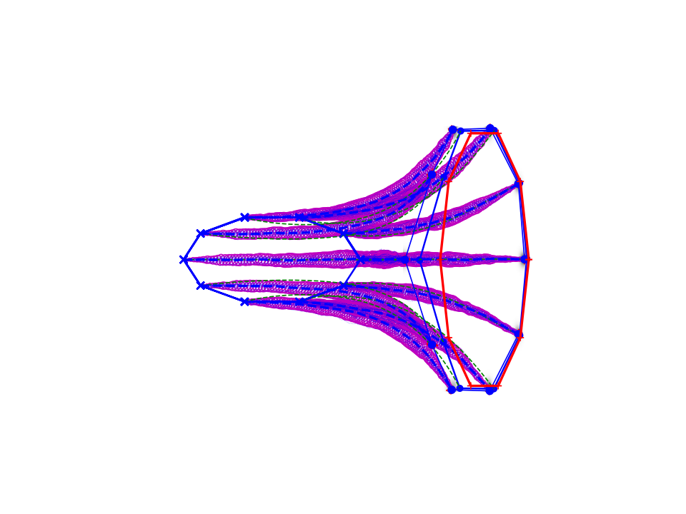
With the setup as Figure 1, we arrange 10 landmarks in two ellipse configurations. We first run the string method (Figure 2, left) and finite temperature string method (Figure 2, right). Samples from the endpoint distributions are shown along with estimated MEP and sample covariance of . The MEP can be compared to the minimizing geodesic between the landmark configurations. The string is at with zero velocity, i.e. for all . The fact that non-zero temperature increases the variance of the string and that the sample covariance increases with time is clearly visible.


Figure 3 shows an example of the convergence of the string with zero temperature, i.e. with single noise realization. The endpoint configuration at converges smoothly as a function of . The final converged string is a perturbed version of the optimal deterministic string.
We now compute the expected mean (5.4) of a new set of sampled configurations shown in Figure 4. The algorithm is initialized with a random configuration, and the evolution of the expected mean configuration can be seen in Figure 5 (left) together with a string matching the mean to a sample (right). The mean converges to what visually appears a to a reasonable mean landmark configuration.
6.2. Left Ventricle Cardiac Outlines


To illustrate the method on non-synthetic data, we perform experiments on landmarks distributed along the outlines of left ventricles on a dataset of 14 cardiac images [SFE01]. Each of the 256256 MRI slices is acquired from 1.0 Tesla whole-body MR scans with ECG-triggered breath-hold sequences. The epicardial and endocardial contours where annotated with 33 landmarks along each outline resulting in 66 landmarks per image. The set of annotations are shown in Figure 6 together with an annotated image. With the higher number of landmarks per outline and the double circular configuration of the landmarks, the matching problem is more difficult than for the synthetic examples.
As in Figure 5, Figure 7 shows results of estimating the mean along with a string connecting the estimated mean to one of the data samples. Initialized with a configuration of landmarks in the centre of the image (blue), the mean converges in a stable way towards the final estimate (red). The energy as a function of for the first 25 iterations is displayed Figure 8. Up to the stochasticity from the sampling, it converges monotonically from its initially high value as the landmarks approach the mean configuration.
6.3. Image Strings
We now use the image equation (4.17) to provide an example of matching with stochastic image strings and the effect of the noise on the image evolution. We here use cubic B-spline kernels for the noise positioned in a grid over the domain with amplitude and length scale set to make the noise amplitude uniform over the domain. Image gradients in the stochastic image flow in (3.4) are computed by finite differences, and the flow field arise from the momentum field by application of the kernel , here again, a convolution with a Gaussian kernel.
In Figure 9, a triangle (, top row, left) is matched to a triangle (, top row, centre) with the stochastic algorithm giving the result in the top row, right. The bottom row shows the evolution of the moving image as a function of the second time variable during the iterations of the matching algorithm. The momentum field and hence the velocity field are initialized to zero at the start of the algorithm. The matching is inexact as can be seen by the triangle protrusion in the matching result that would require a higher warp energy to disappear fully.
The algorithm runs with finite temperature drawing new noise for each iteration. Figure 10 illustrates the effect of the noise after the final iteration of the matching algorithm. The two top rows show the final image string with zero noise as a function of the first time variable , and a magnitude plot of the corresponding velocity field . Notice how the deformation is localized at the edges of the images. Row 3-5 display the image string as a function of for three different noise realizations. Row 6 shows the stochastically perturbed velocity field corresponding to the image flow in row 5. The amplitude is here not concentrated around the edges of the image in contrast to the situation in row 2. The effect of the stochastic perturbations to the flow is substantial. Note that the perturbations are changing during the iterations of the matching algorithm affecting the gradients of the matching terms. However, the averaging over the noise realizations provided by the string method makes the estimated deterministic trajectory stable to these perturbations as seen in the top row of the figure.


7. Conclusion
Shape stochasticity can be introduced to model stochastic shape variation in a way that is compatible with the geometric structure of the LDDMM framework. In this setting, optimal dynamics arise from a matching energy that is dependent on the stochastically perturbed reconstruction equation, or from a constrained and the stochastically perturbed variational principle in the exact matching case. In this paper, we derived the image case of the stochastic EPDiff equations for inexact shape matching, and showed how they extend the vector form of the deterministic EPDiff equation by addition of a Stratonovich perturbation term.
The matching algorithm used in deterministic LDDMM often referred to as the Beg algorithm has a direct counterpart in the stochastic case because the noise is introduced to preserve the momentum equation. We have shown how the stochastic Beg algorithm is a shape equivalent of the string methods used in rare event sampling. The shape string method can be used with both zero and finite temperature.
We provided examples of how the string method can be used for computing statistics of observed data in a computationally efficient way, and we gave examples of the shape string method and string based statistics on finite dimensional landmark manifolds and images equipped with LDDMM geometry. The momentum map representation of shapes [BGBHR11] and the preservation of the momentum map in the stochastic setting allows the method to be applied to other shape data types beyond these examples. One such case would be matching of tensor fields as pursued in Diffusion Tensor MRI where examples of momentum maps for selected choices of actions are given in [BGBHR11]. As for the landmark and image equations, once the momentum map is established, the string update equations follow directly.
Acknowledgements
AA acknowledges partial support from an Imperial College London Roth Award and the EPSRC through award EP/N014529/1 funding the EPSRC Centre for Mathematics of Precision Healthcare. AA and DH are partially supported by the European Research Council Advanced Grant 267382 FCCA held by DH. DH is also grateful for support from EPSRC Grant EP/N023781/1. SS is partially supported by the CSGB Centre for Stochastic Geometry and Advanced Bioimaging funded by a grant from the Villum Foundation. We thank the anonymous reviewers for insightful comments that have substantially improved the manuscript.
References
- [ADCH18] Alexis Arnaudon, Alex L De Castro, and Darryl D Holm. Noise and dissipation on coadjoint orbits. Journal of Nonlinear Science, 28(1):91–145, 2018.
- [AHPS17] Alexis Arnaudon, Darryl D Holm, Akshay Pai, and Stefan Sommer. A stochastic large deformation model for computational anatomy. In Information Processing for Medical Imaging (IPMI), 2017.
- [AHS18] Alexis Arnaudon, Darryl D. Holm, and Stefan Sommer. A Geometric Framework for Stochastic Shape Analysis. accepted for Foundations of Computational Mathematics, arXiv:1703.09971 [cs, math], 2018.
- [BGBHR11] Martins Bruveris, François Gay-Balmaz, Darryl D Holm, and Tudor S Ratiu. The momentum map representation of images. Journal of Nonlinear Science, 21(1):115–150, 2011.
- [BMTY05] M Faisal Beg, Michael I Miller, Alain Trouvé, and Laurent Younes. Computing large deformation metric mappings via geodesic flows of diffeomorphisms. International journal of computer vision, 61(2):139–157, 2005.
- [DLM99] Bernard Delyon, Marc Lavielle, and Eric Moulines. Convergence of a Stochastic Approximation Version of the EM Algorithm. The Annals of Statistics, 27(1):94–128, 1999.
- [DLR77] A. P. Dempster, N. M. Laird, and D. B. Rubin. Maximum likelihood from incomplete data via the EM algorithm. Journal of the royal statistical society, series B, 39(1):1–38, 1977.
- [ERVE02] Weinan E, Weiqing Ren, and Eric Vanden-Eijnden. String method for the study of rare events. Physical Review B, 66(5):052301, August 2002.
- [ERVE05] Weinan E, Weiqing Ren, and Eric Vanden-Eijnden. Finite temperature string method for the study of rare events. The Journal of Physical Chemistry. B, 109(14):6688–6693, April 2005.
- [Fré48] Maurice Fréchet. Les élèments aléatoires de nature quelconque dans un espace distancié. Ann. Inst. H. Poincaré, 10:215–310, 1948.
- [HM05] Darryl D. Holm and Jerrold E Marsden. Momentum maps and measure-valued solutions (peakons, filaments, and sheets) for the epdiff equation. In The breadth of symplectic and Poisson geometry, pages 203–235. Springer, 2005.
- [Hol11] Darryl D. Holm. Geometric Mechanics - Part I: Dynamics and Symmetry. Imperial College Press, London : Hackensack, NJ, 2 edition edition, 2011.
- [Hol15] Darryl D Holm. Variational principles for stochastic fluid dynamics. Proceedings of the Royal Society of London A: Mathematical, Physical and Engineering Sciences, 471(2176):20140963, 2015.
- [HS89] Trevor Hastie and Werner Stuetzle. Principal curves. Journal of the American Statistical Association, 84(406):502–516, 1989.
- [HT16] Darryl D Holm and Tomasz M Tyranowski. Variational principles for stochastic soliton dynamics. Proc. R. Soc. A, 472(2187):20150827, 2016.
- [HZN09] G.L. Hart, C. Zach, and M. Niethammer. An optimal control approach for deformable registration. pages 9–16. IEEE, June 2009.
- [KAS17] Line Kühnel, Alexis Arnaudon, and Stefan Sommer. Differential geometry and stochastic dynamics with deep learning numerics. arXiv:1712.08364, December 2017. arXiv: 1712.08364.
- [MS17] S. Marsland and T. Shardlow. Langevin Equations for Landmark Image Registration with Uncertainty. SIAM Journal on Imaging Sciences, pages 782–807, January 2017.
- [Øk03] Bernt Øksendal. Stochastic Differential Equations: An Introduction with Applications. Springer Science & Business Media, 2003.
- [SFE01] Mikkel Bille Stegmann, Rune Fisker, and Bjarne Kjær Ersbøll. Extending and applying active appearance models for automated, high precision segmentation in different image modalities. Proc. 12th Scandinavian Conference on Image Analysis - SCIA 2001, Bergen, Norway, pages 90–97, 2001.
- [Tib92] Robert Tibshirani. Principal curves revisited. Statistics and Computing, 2(4):183–190, December 1992.
- [TV12] Alain Trouvé and François-Xavier Vialard. Shape splines and stochastic shape evolutions: a second order point of view. Quarterly of Applied Mathematics, 70(2):219–251, 2012.
- [VEV09] Eric Vanden-Eijnden and Maddalena Venturoli. Revisiting the finite temperature string method for the calculation of reaction tubes and free energies. The Journal of Chemical Physics, 130(19):194103, May 2009.
- [Via13] François-Xavier Vialard. Extension to infinite dimensions of a stochastic second-order model associated with shape splines. Stochastic Processes and their Applications, 123(6):2110–2157, 2013.
- [You10] Laurent Younes. Shapes and Diffeomorphisms. Springer, 2010.