Reinforcement Learning based Multi-Access Control and Battery Prediction with Energy Harvesting in IoT Systems
Abstract
Energy harvesting (EH) is a promising technique to fulfill the long-term and self-sustainable operations for Internet of things (IoT) systems. In this paper, we study the joint access control and battery prediction problems in a small-cell IoT system including multiple EH user equipments (UEs) and one base station (BS) with limited uplink access channels. Each UE has a rechargeable battery with finite capacity. The system control is modeled as a Markov decision process without complete prior knowledge assumed at the BS, which also deals with large sizes in both state and action spaces. First, to handle the access control problem assuming causal battery and channel state information, we propose a scheduling algorithm that maximizes the uplink transmission sum rate based on reinforcement learning (RL) with deep Q-network (DQN) enhancement. Second, for the battery prediction problem, with a fixed round-robin access control policy adopted, we develop a RL based algorithm to minimize the prediction loss (error) without any model knowledge about the energy source and energy arrival process. Finally, the joint access control and battery prediction problem is investigated, where we propose a two-layer RL network to simultaneously deal with maximizing the sum rate and minimizing the prediction loss: the first layer is for battery prediction, the second layer generates the access policy based on the output from the first layer. Experiment results show that the three proposed RL algorithms can achieve better performances compared with existing benchmarks.
Index Terms:
Internet of things, energy harvesting, reinforcement learning, access control , battery prediction.I Introduction
The Internet of things (IoT) has a crucial need for long-term or self-sustainable operations to support various applications[1][2]. In recent years, energy harvesting (EH) has been recognized as an emerging technique that may significantly increase the network lifetime and help reduce the greenhouse gas emissions in general wireless applications [3][4][5]. This technology trend provides a promising energy solution for IoT applications [6][7]. Accordingly, EH has been being intensively discussed for supporting the future IoT systems, in D2D communications, wireless sensor networks, and future cellular networks [8][9]. Fundamentally, the amount of harvested energy may be unpredictable due to the stochastic nature of energy sources, i.e., energy arrives at random times and in arbitrary amounts, which poses great challenges to researchers [5][10]. It can be expected that how to handle the dynamics of the harvested energy would be a key design issue in EH based wireless communication systems.
I-A Related Works and Motivations
In general, the related research works on EH based systems could be categorized into two classes based on the availability of the knowledge about energy arrivals. The first class comprises offline approaches that require complete non-causal knowledge of the considered stochastic system, which are usually adopted to derive the performance upper bounds [11][12][13]. In particular, the optimal uplink resource allocation was investigated in [12] for the scenario where two EH users first harvested energy from the wireless signals and then cooperatively sent information to the access point. Also, the optimal packet scheduling over multiple access channels was studied in [13], with the goal of minimizing the time by which all packets from both users are delivered to the destination.
The second class comprises online approaches [14][15][16]. Authors in [14] studied a multi-access wireless system with EH transmitters, and the access problem was modeled as a partially observable Markov decision process (POMDP). In [15], the optimal power control policies for EH nodes in a multi-access system was considered, where a dam model was constructed to capture the dynamics of the EH process. In these approaches, some statistic knowledge regarding the dynamic system should be known at the transmitters [16]. In many practical applications, the complete non-casual knowledge or even statistical knowledge of the system dynamics (including both the channel and energy parts) might not be available, especially when the EH processes are non-stationary or from sources with unknown distributions. For example, in a wireless network with solar EH nodes distributed randomly over a geographical area, the characteristics of the harvested energy at each node depend on the node location, and change over time in a non-stationary fashion [17]. In such cases, the priori knowledge about dynamics of energy sources is very difficult to obtain.
Given the above issues, learning based model-free approaches become more attractive, where the requirements for the priori knowledge are widely relaxed or even removed [18]. In learning based methods, the learning agent may learn certain statistical information about an unknown environment system by interacting [11]. In related works, the point-to-point communication with an EH transmitter was studied in [19] and [20]. Specifically, a Q-learning based theoretic approach was introduced in [19], where the transmitter makes a binary decision, i.e., to transmit or not, in each time slot with the objective of maximizing the total transmitted data. In [20], the authors studied a transmit power allocation policy to maximize the throughput using reinforcement learning (RL) with linear function approximation. The RL algorithm state-action-reward-state-action (SARSA) was combined with non-linear function approximation in [20] to enable the use of incoming energy and channel values, which were taken from a continuous range; thus the authors were able to improve the performance in an EH point-to-point scenario. Unfortunately, the theoretical performance cannot be guaranteed and the learning trends are unstable with non-linear function approximation, as shown in [21].
Given the open nature of wireless systems, there is a crucial need to study the multiuser systems. However, most of the existing works have not provided any stable and efficient learning based approaches for multiuser access control, especially when the state space and action space of the considered system are large. Fortunately, the recently proposed deep Q Network (DQN) technique [22] successfully adapted the deep neural network as a function approximator in Q-learning algorithms dealing with large state spaces [23]. With DQN, there are two major changes to scale Q-learning: the network is trained with mini-batch samples from a replay buffer to minimize the correlations among samples; a target Q network is given to iteratively update the neural network weights [24].
Wireless access control strategies for EH nodes are usually proposed to make the full use of energy and maintain a perpetual lifetime. However, the uncertainty of ambient energy availability poses new challenge to sustainable perpetual operations [25]. Thus, battery level prediction in such EH based systems is also worth investigating since a high battery prediction accuracy could potentially benefit the communication performance. For example, a novel solar energy prediction algorithm with Q-learning based on the weather-conditioned moving average (WCMA) algorithm was proposed in [26]. Unfortunately, this algorithm is restricted to one type of energy sources and suffers from high computation complexity. In [27], an online energy prediction model for multi-source EH wireless sensor networks was proposed, which leverages the past observations to forecast the future energy availability. Nevertheless, this energy prediction model requires that the EH dynamics should be known in advance. On the other hand, instead of studying the access control and battery prediction problems separately in EH based IoT applications, it has great significance to design a joint scheme that feeds the energy prediction results to the access control design, which could lead to better overall system performances. This is the focus of this paper.
I-B Our Contributions
To tackle the aforementioned problems, we focus on an uplink wireless system with EH user equipments (UEs) and one BS, where the BS may only use certain causal information on system dynamics. We first apply a long short-term memory (LSTM) deep Q-network (DQN) based approach to design the UE uplink access control. Then, by fixing the access control policy to be round-robin, we develop a deep LSTM neural network based battery prediction scheme to minimize the prediction loss. Furthermore, we jointly consider the access control and battery prediction problem using a proposed two-layer LSTM based neural network with DQN enhancement. The main contributions are summarized as follows:
- •
We consider an uplink transmission scenario with multiple EH UEs and limited access channels, where neither non-casual knowledge nor statistical knowledge of the system dynamics (including both the channel and energy arrival states) is assumed.
- •
On the condition that only user battery and channel states of the current time slot are known at the BS, we propose an LSTM DQN based algorithm as the UE uplink access control scheme with the objective of maximizing the long-term expected total discounted transmission data. Other than the traditional access control problems that usually consider maximizing the instantaneous sum rate [14], our goal is to achieve a more stable and balanced transmission for a long time horizon.
- •
By fixing the access control policy to be round-robin and assuming that the scheduled users embed the information of their true battery states in the transmission data, we propose a deep LSTM neural network based battery prediction scheme to minimize the prediction loss (defined over the differences between the predicted battery states and the true battery states within the selected UE set).
- •
We develop a joint access control and battery prediction solution by designing a two-layer LSTM DQN network. The first LSTM based neural network layer is designed to generate the predicted battery levels, and the second layer uses such predicted values along with the channel information to generate the access control policy. The two-layer LSTM based network is trained jointly with the combined objective of simultaneously maximizing the total long-term discounted sum rate and minimizing the discounted prediction loss of partial users.
- •
The proposed algorithms are designed with many practical considerations without strong assumptions. In particular, the BS has no prior knowledge on the UEs’ energy arrival distributions. We assume that only the scheduled users embed the information of their true battery states in the transmission data, which greatly reduces the system signaling overheads.
- •
Extensive simulations under different scenarios show that the proposed three algorithms can achieve much better effectiveness and network performance than the various baseline approaches.
The rest of this paper is organized as follows. In Section II, we introduce the system model with some basic assumptions, and also the preliminaries on deep Q-learning and LSTM networks. In Section III, we present the problem formulation for access control, as well as the LSTM DQN based learning algorithm. Section IV studies the battery prediction problem. Furthermore, in Section V, we introduce the joint design problem and its solution. We provide simulation results in Section VI, and finally conclusions in Section VII.
Notations: and denote state and the state at time slot , respectively; and denote action and the action at time slot , respectively; denotes the reward at time slot ; denotes the minimum operator; denotes the expected value given that the agent follows policy ; denotes the operator; denotes the determinant or the cardinality of the set, depending on the context; denotes the -norm; denotes the first-order derivative operator; denotes the space of real matrixes.
II System Model and Preliminaries
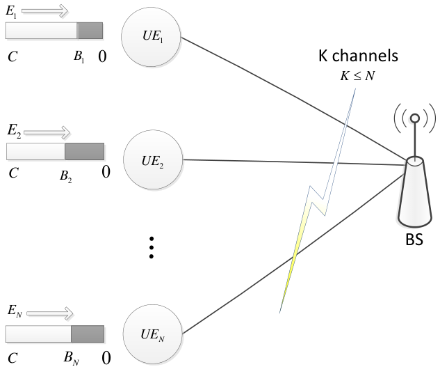
II-A System Model
We consider an uplink wireless system with EH based UEs and one BS, as depicted in Fig. 1. The system operates in a time-slotted fashion with equal-length time slots (TSs), with a normalized slot length equal to one. The BS is able to pick out of the UEs to perform uplink access ( can also be viewed as the number of available orthogonal channels). The set of all the UEs and the selected subset of UEs at TS are denoted by and , respectively, where . We denote the channel power gain between UE and the BS at TS by and let be the set of all the channel gains at TS . We assume that at the beginning of each TS, the instantaneous channel state information (channel power gain) can be obtained at BS. Besides, the channel states remain constant during each TS and may change across different TSs [11]. We assume that the UEs always have data for uplink transmission in each TS. The location of the BS is fixed, while the UEs follow random walks across different TSs and their locations remain unchanged during one TS.
We assume that all the UEs have no other power sources and they only use the harvested energy, which is collected from the surrounding environment via some renewable energy sources (i.e., wind power, solar power or hydropower). Many energy arrival processes based on such sources are shown to be Markov processes [26][27][28], but this is not strictly required in our paper. All the battery states are quantized for analysis convenience [14]. We assume that the battery capacity is , same for all the UEs. We use and to denote the amount of harvested energy and the state of battery for UE at the beginning of TS , respectively. Let denotes the set of all the UEs’ current battery states. We assume that the transmission power for each selected UE is fixed to be [14][19]. After is harvested at TS , it is stored in the battery and is available for transmission in TS . The rechargeable battery is assumed to be ideal, which means that no energy is lost with energy storing or retrieving and the transmission of data is the only source of UE energy consumption. Once the battery is full, the additional harvested energy will be abandoned. We assume that the power required to activate the UE EH circuit is negligible compared with the power used for signal transmission [5][29] [30], since the processing power for EH circuit activation is usually very small compared with the transmit power in practice. For example, as shown in [31], the power consumption for transmission is about 23 times the power consumption for activating the EH circuit.
We use a binary indicator to describe the access control policy: If UE is scheduled to access the channel at TS (i.e., ), ; otherwise, . We use another indicator to denote the transmission status such that: When , , which means that the transmission could be done successfully; otherwise, , which means that at TS , UE cannot transmit data to the BS and the current transmission is failed. Based on the above notations, the battery evolution of UE over different time slots could be described as:
| (1) | ||||
| (2) |
II-B Preliminaries: Deep Q-Learning and LSTM
In this subsection, we briefly introduce the RL network that is used in this paper to solve the access control and battery prediction problems. The detailed physical meanings of the notations in the RL network will be introduced later. RL is developed over the Markov decision process (MDP) formulation, which includes: a discrete state space , an action space , an immediate reward function and a transition probability set where satisfies the Markov property , where , and denote the state, action and reward at TS , respectively.
Note that our paper studies a multiuser uplink scenario. When we use MDP to model such a system, the number of system states is large since the state contains the channel gain and battery level for every UE, and the size of corresponding action space is also large as it is proportional to the number of UEs.
Based on the MDP formulation, the general goal of an RL agent is to find a good policy, which is a function mapping from state space to the action space, denoted by . In this paper, the RL agent is the BS, whose goal is to maximize/minimize the reward/loss in the long run by following the optimal policy. The total discounted reward from TS onwards can be written as:
| (3) |
where is the discount factor.
For a typical RL network, the state value function and action value function are instrumental in solving the MDP, which are defined as
| (4) |
| (5) |
where denotes the expected value given that the agent follows policy [32].
The optimal policy is the policy that can maximize (4) at any state, and we can observe from (4) and (5) that . The corresponding action-value function for the optimal policy is denoted by . A fundamental property of the value functions is that the functions can be evaluated in a recursive manner by using the Bellman equations. The general form of the Bellman optimality equation for the action value function is given as
| (6) |
where is the expected value of the next reward given the current state and action , together with the next state [32].
In a system with large state and action spaces, it is often impractical to maintain all the Q-values, i.e., all the function values in (5) for all possible state-action pairs. Generally, nonlinear function approximation for learning (Q-learning) is a popular approach [20]. However, it usually cannot provide theoretical guarantees, producing unstable trajectories in many practical applications. Fortunately, the recently proposed DQN [22] successfully adapts the deep neural network as a function approximator in Q-learning over large state spaces. In our work, we adopt the DQN to approximate the action value function for all state action pairs.
In particular, we build the DQN based on Long Short-Term Memory (LSTM), which is a special recurrent neural network that can connect and recognize long-range correlated patterns over the input and output states. Specifically, an LSTM network is considered as multiple copies of the memory blocks (LSTM units), each of which passes a message to its successor as shown in Fig. 2. Such an LSTM unit has four gates to control the flow of information. With the input from the current step and the hidden state of the previous step , the unit firstly decides what information to throw away through multiplying the forget gate output by the cell state from . The cell state runs straight down all the units in the LSTM network. The next procedure is to decide what new information is going to be stored in the cell state using the input gate and cell gate. Finally, the hidden state is updated with the new cell state and the output of the output gate.
II-C Performance Metric
In this paper, we adopt two main metrics to measure the overall performance of the network. The first is the sum rate of all the uplink transmissions to the BS. At time slot , the network uplink sum rate at the BS is given by
| (7) |
where is the spectrum bandwidth and is the noise power [33].
The second metric is the prediction loss, which is the dissimilarity between the predicted battery states and the true battery states. It is worth mentioning that in our battery prediction design, the BS does not know the full information of (i.e., the battery states at each TS) for decision making. In order to avoid large signaling overheads for reporting battery states to the BS at each TS, only the selected UEs send their true battery states along with transmitted data to the BS. Thus, the instantaneous prediction loss only involves the selected UE set. However, as the RL algorithm explores all the UEs, all the UEs will be taken into account in the long run. The instantaneous prediction loss at time slot is given by
| (8) |
where and are the predicted battery state and true battery state of UE at time slot , respectively.
III Access Control with RL
In this section, we consider the access control problem described in Fig. 1. It is assumed that the BS and UEs are cooperative such that the BS may obtain the knowledge of current channel gains and UEs’ current battery states [11]. The system operates as follows. When the system enters a new time slot, the BS uses the current UE battery states and channel information to compute its scheduling policy for the current TS with a RL network, and then broadcasts the policy to all the UEs. Afterwards, the selected UEs transmit their data to the BS with transmission power , while those who are not selected remain idle. All the UEs execute the energy conversion process and store the energy into the battery for the future use. The above process repeats in the next TS.
III-A Problem Formulation
The BS needs to find a good access control policy with the objective of maximizing the long-term expected uplink sum rate. In TS , the system state contains two parts: the current channel state information and the current UE battery state . That is, we have . The action space contains all the possible UE selection choices, i.e., , with , . Here, the reward signal is the received sum rate at the BS, which is regarded as the reward at state by taking action . The description of is shown in (7) and the total discounted sum rate (reward) can be calculated as
| (9) |
Our learning goal is to maximize the expected cumulative discounted reward by following the access policy from a starting state, which is given by
| (10) |
As such, the access control optimization problem can be formulated as
| (11a) | ||||
| (11b) | ||||
| (11c) | ||||
III-B LSTM-DQN based Access Control Network
In this subsection, we present the proposed learning framework and algorithm of uplink access control to solve problem (11). In Fig. 3, we illustrate the architecture of our LSTM-DQN network for access control. The centralized controller at the BS receives the state information at the beginning of each TS. With the input , the entire layer of the LSTM network outputs the approximated Q-value in mini-batch , where is the size of the action space and . Then, we use a fully connected network layer to adjust the size of the Q-value vector to make it fit the action space, i.e., . We use to represent our neural network in Fig. 3 with the input as the system state and the output as . Here, denotes the set of network weights which contains: the LSTM layer parameters and the fully connected network layer parameters , where is the number of LSTM units.
In the learning time slot , is estimated by . We recall that given , with at hand the BS selects that achieves the maximum , and the optimal policy is the greedy policy if can be perfectly estimated. However, the greedy policy is not optimal before the estimate of is accurate enough. In order to improve such estimates, the BS should balance the exploration of new actions and the exploitation of the known actions. In exploitation, the BS follows the greedy policy; in exploration the BS takes actions randomly with the aim of discovering better policies. The balance could be realized by the -greedy action selection method [34] (as given later in Algorithm 1) at each time slot, which either takes actions randomly to explore with probability or follows the greedy policy to exploit with probability , where .
After executing the selected action , the BS receives the reward and the system changes to the new state. We utilize experience replay to store the BS’s experiences at each TS, which is denoted by tuple in a data-set . The replay memory size is set to be , which means their we could store experience tuples. Here, is generated by the control policy . In each TS, instead of updating based on transitions from the current state, we randomly sample a tuple from . Updating network parameters in this way to avoid issues caused by strong correlations among transitions of the same episode [22]. We parameterize an approximate value function using the proposed learning network in Fig. 3 with network parameters (weights) of . With the sampled transitions, is the target Q-value with network weights obtained from previous iteration. Accordingly, we have the following loss function to minimize:
| (12) |
Differentiating the loss function with respect to the weights, we arrive the following gradient:
| (13) |
where denotes the gradient vector of with respect to . By adopting the routine of stochastic gradient descent [22], the overall access control algorithm is summarized in Algorithm 1.
IV Battery Prediction with RL
In wireless EH network, it is important to keep energy-neutral, i.e., energy expenditure equals the harvested amount and operation permanently. An effective energy-neutral policy may benefit from an accurate prediction for the future harvested energy. In this section, we consider reusing a similar LSTM method to the one used in the previous section for UE battery state prediction. In our design, we do not need to know the UE energy model, as the method is purely data driven.
IV-A Problem Formulation
For the EH system in Fig. 1, we assume that the access control policy is fixed to be the widely used round-robin scheduling policy [14]. At the beginning of each TS , the LSTM based predictor can output the predicted battery states . The BS then schedules the UE transmission based on round-robin scheduling and broadcasts the schedule to all the UEs. After receiving the schedule, the selected UEs transmit data to the BS, along with their current ground-truth battery states [14]. We use the difference between the predicted battery states and the true battery states within the selected UE set as the performance metric for the designed predictor, as shown in (8).
A memory component with a history window of is equipped at the BS to store limited history information. At TS , the state space contains three parts: the access scheduling history information , where and ; the history of predicted UE battery information , where and ; and the history of selected UE true battery information , where and .
We use , to denote the system state, and to denote the battery prediction result, which is also called the prediction value . We denote the predicted battery states of selected UEs as vector with elements and the received true battery states of selected UEs as vector with elements . Thus, the prediction loss in (8) is equivalent to
| (14) |
The long-term prediction performance, i.e., the total discounted prediction loss, is given by
| (15) |
The goal of the learning algorithm is to obtain the optimal prediction policy to minimize the cumulative discounted loss, which is given by
| (16) |
The battery prediction problem can be formulated as
| (17a) | ||||
| (17b) | ||||
IV-B Deep LSTM based Battery Prediction Network
In Fig. 4, we illustrate the architecture of our LSTM based prediction network, which is denoted as the prediction generator. At the beginning of TS , the BS first observes and imports it into the LSTM network layer, and the LSTM network outputs the predicted battery states in multi mini-batch . Then we use a fully connected network layer to adjust the size of the LSTM output vector as . The BS then announces the access policy based on round-robin. After UEs’ transmissions, the BS receives the true battery states . We use to denote the prediction generator with the input , and the output . Here, is the set of network weights, which contains the LSTM layer parameters and the fully connected layer parameters , where is the number of LSTM units.
A good policy in this case is the one minimizing the cumulative discounted prediction loss based on the observed states. We utilize experience replay (defined in previous Section) to store the BS experiences . In each TS, we randomly sample a tuple from to update the network parameters . Stochastic gradient descent is used to minimize the prediction loss by adjusting the network weight parameter after each sample in the direction that would reduce the loss the most. The weights are updated as
| (18) |
where is a positive step size, is the parameterized prediction values with the network parameters , and denotes the gradient vector of with respect to , and is the target output of the th training step. We adopt the temporal-difference (TD) policy evaluation algorithm [32], i.e., , where the TD error is described as
| (19) |
The updating in (18) can be executed as . The battery prediction algorithm based on the deep LSTM network is summarized in Algorithm 2.
V Jointly Access Control and Battery Prediction Based on RL
By jointly considering the access control and battery prediction, we could relax the requirements of the knowledge on the UE battery states of the current TS for access control, which means that only current channel gains are needed at the BS at each TS.
In particular, we propose a two-layer LSTM based DQN control network, which is applied at the BS and operates as follows. At the beginning of each TS , the first LSTM based network layer, which is used for battery prediction, outputs all the UEs’ predicted battery states based on the history information. The predicted battery states are then input to the second layer, which is designed to generate the access control policy. Next, with the output of the second layer, i.e., the access control policy, the BS broadcasts the schedule to all the UEs. Afterwards, the selected UEs execute the policy and transmit their data to the BS, along with their current true battery states , which will be stored into the history information for future prediction usage; those UEs who are not selected remain idle. The BS finally receives rewards, i.e., the mixture of the sum rate and the prediction loss. All the UEs complete the energy conversion and store the energy to the battery for future use. The above process repeats in the next TS.
V-A Problem Formulation
The BS operates as the centralized controller that predicts the UE battery states and schedules the subset of users to access the uplink channels at each TS. At TS , the whole system state is denoted as . We deploy a memory component with a window of at the BS to store the history data, which contains: the access scheduling history information, i.e., access indicators, , where and ; the history of predicted UE battery information , where and ; and the history of the true battery information within the selected UE sets , where and . The channel gain at TS is . Thus, we have . Given and the scheduling policy , the action is derived with the DQN control network given in Fig. 5.
Since the performance of the joint solution relies on both the access control policy and battery prediction results, the immediate reward contains the received sum rate in (7) and the battery prediction loss in (8), which is regarded as the penalty to the sum rate. The immediate reward received at TS of state by taking action in the joint solution is set as
| (20) | ||||
where denotes the penalty factor for balancing two different physical quantities. The long-term system performance, i.e., total discounted reward, from TS onwards, is given by
| (21) |
The objective of our joint learning algorithm is to obtain the optimal scheduling policy to maximize the cumulative discounted reward is given by
| (22) |
The joint problem can then be formulated as
| (23a) | ||||
| (23b) | ||||
| (23c) | ||||
V-B Two-Layer LSTM-DQN based Joint Network
In this subsection, we present the proposed learning RL network and the algorithm to solve problem in (23), where Fig. 5 shows the architecture of the proposed new hybrid control network combining the LSTM neural network and deep Q-learning enhancement.
The network in Fig. 5 can be divided into two layers. The first is the LSTM layer based network to perform the battery prediction, which is called the prediction generator. In a practical scenario with unknown energy sources, the BS has no information about the UE EH processes and battery states. At the beginning of TS , the input of the prediction generator is the history knowledge within certain time window, which contains: , and . We denote the input as , . With , the first LSTM network outputs the predicted battery states in multi mini-batch . Then a fully connected network follows to adjust the size of the LSTM output vector to be the expected . We use to denote the prediction generator with the input and the output . Here, the set of network weights contains the LSTM network parameters and the fully connected network parameters , where is the number of LSTM units.
The second layer is the action generator for producing the access control policy, which contains an LSTM layer and a fully connected layer. At TS , the input of the action generator contains: the output values of , i.e., ; and the current channel states . We denote the input of the action generator as . With , the LSTM layer outputs the approximated Q-value in mini-batch , where is the size of the action space with . Then, the fully connected network layer adjusts the size of the Q-value vector to . Finally, the action generator outputs the approximated Q-value . We represent the action generator as with the input and the output . Here, is the set of network weights containing the LSTM layer parameters and the fully connected layer parameters .
Therefore, by combining the prediction generator and action generator, the proposed two-layer LSTM-DQN based joint network can be represented as with the entire input as and the output approximation of Q-value as .
In the proposed RL network, we learn the parameters of the prediction generator and of the action generator jointly. The parameters of the two-layer joint network is denoted by . At the beginning of TS , the BS receives . The prediction generator firstly outputs , and the BS then stores by updating its history memory. With the predicted battery states and channel gains, the action generator then outputs the Q-value . As explained in Section III, the balance between the exploration of new actions and the exploitation of the known actions is realized by the -greedy action selection method [34]. With -greedy, the BS either takes actions randomly with probability or follows the greedy policy (chosing the action by ) with probability , where .
After executing the selected action , the BS receives the immediate reward . We keep tracking the BS’s previous experience in a replay memory data set , with . Instead of performing updates to the Q-values using transitions from the current episode, we sample a random transition from [22]. Following the Q-learning approach, we obtain the target Q-value , where is the parameterized approximate value function with network parameters obtained from the previous iteration.
We can get the following loss function to minimize:
| (24) |
The updates on can be performed using the stochastic gradient of . It is worth mentioning that, in this gradient, contains both two-layer network parameters, i.e., , which means that the prediction generator and access control policy network are trained in a joint way [35][36]. The overall joint access control and battery prediction algorithm is summarized in Algorithm 3.
VI Simulation Results
In this section, we demonstrate the performance of the two proposed RL based algorithms by simulations. All the results are performed in a simulated LTE uplink scenario with one BS and 30 randomly walking UEs with the speed of . The UEs’ energy arrival processes are modeled as Possion arrival processes with different arrival rates. The cell range is with , where is the transmission distance [37]. The system total bandwidth is and the penalty factor is . All the battery states are quantized into integer units with 5dBm per unit and the transmit power is at 2 units.
The LSTM network consists of 128 units and the fully connected layer uses a tanh activation function. The learning rate is fixed as and the discount factor is set to be . We train the deep RL network with a mini-batch size of 16 and a replay buffer size of . All simulation results are obtained based on the deep learning framework in TensorFlow 1.2.1.
To compare the performance of our proposed algorithms, we consider the following alternative approaches: 1) an offline benchmark provides an upper bound where the BS is assumed to have perfect non-causal knowledge on all the random processes; 2) a myopic policy (MP), which is a widely used data-driven approach in the multi-armed bandit model [14]; 3) the round-robin scheduling; and 4) random scheduling. It is worth mentioning that the presented rewards are averaged by taking the mean over a fixed moving reward subset with a window of 200 training steps to achieve smoother and more general performance comparison.
Firstly, we investigate the performance of Algorithm 1 compared with other methods. As shown in Fig. 6, the proposed learning algorithm always achieves a higher average reward than round-robin and random scheduling. This is intuitive since round-robin only considers the access fairness among all the UEs, and random selection makes the decision even more blindly. With the increase of training steps, the proposed DQN scheme at first stays in an unstable exploration stage. Then, it gradually outperforms MP after training steps. Finally, it converges and becomes stable. This is because that MP always focus on the current sum rate optimization based on the battery beliefs[14], while the DQN algorithm takes the long-term performance into consideration, resulting in a more efficient resource utilization and higher sum rate. Furthermore, we observe that the performance gap between our proposed algorithm and the offline upper bound gets smaller as the training step increases. We also compare the average sum rates under different numbers of available channels and battery capacities. We can also see from Fig. 6 that after getting stable, the average reward of the proposed DQN based algorithm achieves a value that is higher than that with the MP approach, higher than the round-robin approach, and higher than the random scheduling approach. Meanwhile, the average reward of the proposed DQN based approach is lower than the upper bound (i.e., the offline scheduling). It can be seen in Fig. 7 that the proposed DQN algorithm always beats the counterparts when the number of available channels changes from 2 to 20 and the battery capacity changes from 5 to 10 units. Furthermore, the average sum rate increases with the number of available channels. By increasing the battery capacity from 5 to 10 units, the battery overflow is reduced, which results in a higher average sum rate.
For Algorithm 2, we perform simulations for the total battery prediction loss of all the UEs with the proposed DQN algorithm, shown in Fig. 8. It can been seen from Fig. 8(a) that the prediction loss is quite large at the beginning. With the increase of training steps, the loss becomes smaller and goes to a stable value after about 1000 training steps. We zoom in over the loss values between 1000 and 2000 training steps in Fig. 8(b). The average UE battery prediction loss shown in Fig. 8 is about 0.0013 units. It is obvious that the prediction loss is small enough and the proposed deep LSTM prediction network provides good prediction performance.
At last, the performance of the proposed joint scheme in Algorithm 3 is investigated. The average sum rate and the corresponding battery prediction loss are shown in Fig. 9 - Fig. 11, respectively. It can be seen from Fig. 9 that the data-drive approaches, i.e., MP and DQN, always perform better than the round robin and random scheduling, which is intuitive and obvious since the last two have no consideration over sum rate optimization. The proposed DQN based algorithm stays in an exploration stage at the beginning, which is unstable and resulting in a worse performance compared with the MP approach. With more training steps, as expected, the average sum rate of the proposed DQN algorithm arises to be better than MP and remains stable after about training steps. Compared with the offline upper bound, we can observe that though the average sum rate of the proposed DQN cannot achieve the upper bound, the performance gap between the two gets smaller as the training step increases. It can be seen in Fig. 9 that after getting stable, the average reward of the proposed joint algorithm is higher than that of the MP approach, higher than the round-robin approach, higher than the random scheduling approach, and lower than the offline scheduling. The average sum rates under different numbers of available channels and battery capacities are shown in Fig. 10. It can be observed that the proposed DQN algorithm always defeats the MP, round-robin and random approaches when the number of available channels changes from 2 to 20 and the battery capacity changes from 5 to 10 units. Besides, it is obvious that the average sum rate of the proposed DQN algorithm is close to the upper bound. Furthermore, we see that the average sum rate increases with the increase of battery capacity and the number of available channels, owing to the reduction of battery overflow.
The performance of the corresponding battery prediction network for the joint scheme is shown in Fig. 11. Compared with Fig. 9, we see that the battery prediction loss goes to a stable stage earlier than the average sum rate. This is because that the output of battery prediction network is the main input for the access control network; only after the battery prediction is accurate enough, the BS could generate good scheduling policies that achieve high sum rates. It can been seen from Fig. 11 (a) that the prediction loss is quite large at the beginning, becomes smaller as the training step increases, and gets stable after about 22000 training steps. We zoom into the loss values from the 30000th to 32000th training steps in Fig. 11 (b). The average UE battery prediction loss shown in Fig. 11 is about 0.0175 units. It is obvious that the prediction loss is small enough and the proposed deep LSTM prediction network provides good prediction values.
VII Conclusion
In this paper, we developed three RL based methods to solve the user access control and battery prediction problems in a multi-user EH based communication system. With only causal information regarding the channel and UE battery states, the LSTM-DQN based scheduling algorithm was designed to find the optimal policy with the objective of maximizing the long-term discounted uplink sum rate, driven by only instantaneous system information. The battery state prediction algorithm based on deep LSTM was proposed to minimize the prediction loss. Furthermore, the joint problem was considered, where we proposed a two-layer LSTM based network which is trained jointly with deep Q-learning to maximize the long-term discounted sum rate and minimize the cumulative battery prediction loss simultaneously. The simulation results under different conditions were also provided to illustrate the effectiveness of our proposed RL based methods.
References
- [1] P. Kamalinejad, C. Mahapatra, Z. Sheng, S. Mirabbasi, V. C. Leung, and Y. L. Guan, “Wireless energy harvesting for the internet of things,” IEEE Commun. Mag., vol. 53, no. 6, pp. 102–108, June 2015.
- [2] Z. Ni, R. V. Bhat, and M. Motani, “On dual-path energy-harvesting receivers for IoT with batteries having internal resistance,” IEEE Internet Things J., pp. 1–1, Mar. 2018.
- [3] S. Ulukus, A. Yener, E. Erkip, O. Simeone, M. Zorzi, P. Grover, and K. Huang, “Energy harvesting wireless communications: A review of recent advances,” IEEE J. Sel. Areas Commun., vol. 33, no. 3, pp. 360–381, Mar. 2015.
- [4] W. Wang, R. Wang, H. Mehrpouyan, N. Zhao, and G. Zhang, “Beamforming for simultaneous wireless information and power transfer in two-way relay channels,” IEEE Access, vol. 5, no. 6, pp. 9235–9250, May. 2017.
- [5] M. Chu, B. He, X. Liao, Z. Gao, and V. C. Leung, “On the design of power splitting relays with interference alignment,” IEEE Trans. Commun., vol. 66, no. 4, pp. 1–12, Dec. 2017.
- [6] D. T. Thien D. Nguyen, Jamil Y.Khan, “A self-sustainable RF energy harvesting algorithm for WSN-based IoT applications,” in Proc. IEEE GlobeCom, Singapore, Dec. 2017, pp. 168–172.
- [7] Z. Yang, W. Xu, Y. Pan, C. Pan, and M. Chen, “Energy efficient resource allocation in machine-to-machine communications with multiple access and energy harvesting for IoT,” IEEE Internet Things J., vol. 5, no. 1, pp. 229–245, Nov. 2017.
- [8] K. Han and K. Huang, “Wirelessly powered backscatter communication networks: Modeling, coverage, and capacity,” IEEE Trans. Wireless Commun., vol. 16, no. 4, pp. 2548–2561, Apr. 2017.
- [9] K. Tutuncuoglu and A. Yener, “Optimum transmission policies for battery limited energy harvesting nodes,” IEEE Trans. Wireless Commun., vol. 11, no. 3, pp. 1180–1189, Mar. 2012.
- [10] J. Ren, J. Hu, D. Zhang, H. Guo, Y. Zhang, and X. Shen, “RF energy harvesting and transfer in cognitive radio sensor networks: Opportunities and challenges,” IEEE Commun. Mag., vol. 56, no. 1, pp. 104–110, Jan. 2018.
- [11] A. Ortiz, H. Al-Shatri, T. Weber, and A. Klein, “Multi-agent reinforcement learning for energy harvesting two-hop communications with full cooperation,” arXiv preprint arXiv:1702.06185, Feb. 2017.
- [12] X. Di, K. Xiong, P. Fan, H.-C. Yang, and K. B. Letaief, “Optimal resource allocation in wireless powered communication networks with user cooperation,” IEEE Trans. Wireless Commun., vol. 16, no. 12, pp. 7936–7949, Dec. 2017.
- [13] J. Yang and S. Ulukus, “Optimal packet scheduling in a multiple access channel with energy harvesting transmitters,” J. Commun. and Netw., vol. 14, no. 2, pp. 140–150, Apr. 2012.
- [14] P. Blasco and D. Gunduz, “Multi-access communications with energy harvesting: A multi-armed bandit model and the optimality of the myopic policy,” IEEE J. Sel. Areas Commun., vol. 33, no. 3, pp. 585–597, Mar. 2015.
- [15] M. B. Khuzani and P. Mitran, “On online energy harvesting in multiple access communication systems,” IEEE Trans. Inf. Theory, vol. 60, no. 3, pp. 1883–1898, Mar. 2014.
- [16] P. Blasco, D. Gunduz, and M. Dohler, “Low-complexity scheduling policies for energy harvesting communication networks,” in Proc. IEEE ISIT, Istanbul, Turkey, July 2013, pp. 1601–1605.
- [17] C. Wang, J. Li, Y. Yang, and F. Ye, “Combining solar energy harvesting with wireless charging for hybrid wireless sensor networks,” IEEE Trans. Mobile Comput., vol. 17, no. 3, pp. 560–576, Mar. 2018.
- [18] P. Sakulkar and B. Krishnamachari, “Online learning schemes for power allocation in energy harvesting communications,” IEEE Trans. Inf. Theory, pp. 1–1, Nov. 2017.
- [19] P. Blasco, D. Gunduz, and M. Dohler, “A learning theoretic approach to energy harvesting communication system optimization,” IEEE Trans. Wireless Commun., vol. 12, no. 4, pp. 1872–1882, Apr. 2013.
- [20] A. Ortiz, H. Al-Shatri, X. Li, T. Weber, and A. Klein, “Reinforcement learning for energy harvesting point-to-point communications,” in Proc. IEEE ICC, Kuala Lumpur, Malaysia, May. 2016, pp. 1–6.
- [21] G. J. Gordon, “Reinforcement learning with function approximation converges to a region,” in Proc. NIPS, San Francisco, USA, Nov. 2001, pp. 1040–1046.
- [22] V. Mnih, K. Kavukcuoglu, D. Silver, A. A. Rusu, J. Veness, M. G. Bellemare, A. Graves, M. Riedmiller, A. K. Fidjeland, G. Ostrovski et al., “Human-level control through deep reinforcement learning,” Nature, vol. 518, no. 7540, pp. 529–534, Feb. 2015.
- [23] V. Mnih, K. Kavukcuoglu, D. Silver, A. Graves, I. Antonoglou, D. Wierstra, and M. Riedmiller, “Playing atari with deep reinforcement learning,” arXiv preprint arXiv:1312.5602, Dec. 2013.
- [24] S. Gu, T. Lillicrap, I. Sutskever, and S. Levine, “Continuous deep Q-learning with model-based acceleration,” in Proc. Intl. Conf. on Machine Learning, New York, USA, June 2016, pp. 2829–2838.
- [25] M. Deruyck, D. Renga, M. Meo, L. Martens, and W. Joseph, “Accounting for the varying supply of solar energy when designing wireless access networks,” IEEE Trans. on Green Commun. and Netw., vol. 2, no. 1, pp. 275–290, Mar. 2018.
- [26] S. Kosunalp, “A new energy prediction algorithm for energy-harvesting wireless sensor networks with Q-learning,” IEEE Access, vol. 4, no. 7, pp. 5755–5763, Sep. 2016.
- [27] A. Cammarano, C. Petrioli, and D. Spenza, “Online energy harvesting prediction in environmentally powered wireless sensor networks,” IEEE Sensors J., vol. 16, no. 17, pp. 6793–6804, Sep. 2016.
- [28] H. U. Yildiz, V. C. Gungor, and B. Tavli, “A hybrid energy harvesting framework for energy efficiency in wireless sensor networks based smart grid applications,” in 2018 17th Annual Mediterranean Ad Hoc Networking Workshop (Med-Hoc-Net). Capri, Italy: IEEE, June 2018, pp. 1–6.
- [29] A. A. Nasir, X. Zhou, S. Durrani, and R. A. Kennedy, “Relaying protocols for wireless energy harvesting and information processing,” IEEE Trans. Wireless Commun., vol. 12, no. 7, pp. 3622–3636, Jul. 2013.
- [30] R. Zhang, J. Wang, Z. Zhong, C. Li, X. Du, and M. Guizani, “Energy-efficient beamforming for 3.5 GHz 5G cellular networks based on 3D spatial channel characteristics,” Elsevier Comput. Commun., vol. 121, no. 5, pp. 59–70, Mar. 2018.
- [31] X. Zhou, B. Bai, and W. Chen, “Greedy relay antenna selection for sum rate maximization in amplify-and-forward mimo two-way relay channels under a holistic power model,” IEEE Trans. Wireless Commun., vol. 19, no. 9, pp. 1648–1651, Jun. 2015.
- [32] R. S. Sutton and A. G. Barto, Reinforcement learning: An introduction, 2nd ed. MIT press Cambridge, 2014.
- [33] S. Verdu, “Fifty years of shannon theory,” IEEE Trans. Inf. Theory, vol. 44, no. 6, pp. 2057–2078, Apr. 1998.
- [34] K. Narasimhan, T. Kulkarni, and R. Barzilay, “Language understanding for text-based games using deep reinforcement learning,” arXiv preprint arXiv:1506.08941, June 2015.
- [35] K. Cho, B. Van Merriënboer, C. Gulcehre, D. Bahdanau, F. Bougares, H. Schwenk, and Y. Bengio, “Learning phrase representations using RNN encoder-decoder for statistical machine translation,” arXiv preprint arXiv:1406.1078, June 2014.
- [36] T. Mikolov, S. Kombrink, L. Burget, J. Černockỳ, and S. Khudanpur, “Extensions of recurrent neural network language model,” in Proc. ICASSP, Prague, Czech Republic, May. 2011, pp. 5528–5531.
- [37] R. Zhang, X. Jiang, T. Taleb, B. Li, H. Qin, Z. Zhong, and X. Zhang, “Connecting a city by wireless backhaul: 3d spatial channel characterization and modeling perspectives,” IEEE Commun. Mag., vol. 55, no. 5, pp. 62–69, May. 2017.