Learning universality and scaling from simple deposition models
Abstract
We use deposition models of kinetic roughening of a growing surface to introduce the concepts of universality and scaling and to analyze the qualitative and quantitative role of different parameters. In particular, we focus on two classes of models where the deposition is accompanied by a local relaxation process within a distance . The models are in the Edwards-Wilkinson universality class, but the role of is nontrivial.
I Introduction
Kinetic roughening is a widespread phenomenon that is related to the dynamics of a driven interface in the presence of noise. The latter makes the interface rough; that is, the mean square deviation of the interfacial position diverges at large temporal and spatial scales. Examples of driven interfaces include flame fronts, wetting fronts, magnetic domain walls, and the growing front of a bacterial colony.[1, 2, 3] In this paper we study the dynamics of the interface between a solid and a vacuum phase when particles are deposited ballistically onto a growing surface. Ballistic deposition means that particles arrive following a straight trajectory, normal to the average orientation of the surface to avoid shadowing effects. This situation is qualitatively different from a solid phase that is in contact with a gas phase, because in the latter case particles undergo a diffusion process, which gives rise to a nonlocal growth process whose morphology resembles diffusion limited aggregation.[4]
To be specific and to keep the notation simple, we consider a one-dimensional discrete interface defined by the local height , where and are integers. The roughness , which depends on the time and the size of the growing interface, is defined as the square root of the variance of the height,
| (1) |
where the horizontal bar means a spatial average, , and the brackets denote the average over noise.
The models of deposition plus relaxation that we will consider can be summarized by the following algorithm:
- 1.
Choose a random deposition site between 1 and .
- 2.
Apply a relaxation rule to choose the incorporation site in the interval . Use periodic boundary conditions such that .
- 3.
Increment the height of the incorporation site, .
The models to be discussed differ in the relaxation rule (2) and the value of the interval . A random integer among values, , is obtained from a random number generator that returns a random real number in the interval by the relation , where INT means the integer part.
In a deposition model, there are deterministic and random ingredients. In this paper the initial configuration is always a flat surface of zero height, . Alternatively, we can use an initial surface with some roughness, which could be deterministic (such as a pyramidal profile) or a surface with some degree of randomness. The asymptotic form of is independent of the initial configuration (see the Appendix). It is straightforward to see that step (1) is random and step (3) is deterministic; step (2) is mainly deterministic, but with a random component that is necessary (as we will see) to break a tie without breaking a symmetry.
II Models and scaling function
We will consider a downward funnelling model and a minimum model,[5] as illustrated in Fig. 1. In the downward funnelling model (DFM) the deposited particle may reduce its height by moving to a neighboring site for a maximum of hops. If both neighbors of the deposition site have a lower height, a random choice is made. In the minimum model (MIN), the particle is incorporated at the site of minimum height within the interval . For equivalent minima, one site is chosen at random. We see that step (2) is deterministic and randomness is invoked when there are equivalent incorporation sites.

We highlight in Fig. 2 several general features of the roughness for the downward funnelling model with . For fixed , there is an initial temporal regime during which increases with time , followed by a second, stationary regime for during which saturates. The crossover time increases with , and the saturation value increases as well. The log-log plots in Fig. 2 suggest two power laws, and , where is the roughness exponent and is the growth exponent. The crossover time can be derived from the relation ; that is, , which defines the dynamical exponent . From the simulation results we conclude that
| (2) |
where the subscript DF1 denotes the downward funnelling model with .
If we rescale time with respect to the crossover time and rescale the roughness with respect to its saturation value, we obtain data collapse because curves for different values of now lie on the same curve as shown in Fig. 3. These results suggest the following scaling form for the roughness,[6, 7, 8]
| (3) |
with
| (4) |
The relation (3) means that if we rescale space by the factor , it is possible to rescale time and the height of the interface so as to preserve Eq. (3). To see this scaling note that if , the constancy of the argument of the function (necessary because is not an homogeneous function) requires that , and acquires the factor . According to the definition of the roughness in Eq. (1), this factor is equivalent to rescaling the height as .


The growing interface is therefore self-similar so that if we do a suitable magnification of a snapshot of the surface in the stationary regime , the enlarged image is statistically equivalent to the interface itself. Otherwise, a suitable magnification of the snapshot is statistically equivalent to the interface at a different time. The only condition is that we must consider large temporal and spatial scales, , in the same way that scaling appears near the ferro–paramagnetic phase transition in the Ising model. [9, 10]
III Universality
In analogy with continuous thermal phase transitions, we expect that certain features of the deposition model are irrelevant; that is, the roughness exponents and the function do not change. To check this expectation, we plot as a function of for DF1, DF10, MIN1, and MIN2 (DF10 refers to the DF model with , and similar notation for the MIN models).

The results show that the DF and MIN models have the same exponents, because after rescaling the four models we have considered, they exhibit the same initial slope (therefore the same exponent ) and asymptotically goes to a constant and therefore they have the same exponent . The residual differences among models are non-universal features, which we will discuss in Sec. IV.
The models we have introduced belong to the same Edwards-Wilkinson (EW) universality class.[11, 8, 12] Its large scale properties are described by the homogeneous, linear stochastic differential equation[11]
| (5) |
where indicates white noise whose properties can be formally written as
| (6a) | ||||
| (6b) | ||||
In the Appendix we give a short analytical derivation of the scaling function and of the roughness exponents for the Edwards-Wilkinson equation, which are equal to
| (7) |
Rather than discussing the exact form of the scaling function, we will consider the Edwards-Wilkinson equation itself and discuss which features are relevant or irrelevant. We first note that the continuum height in Eq. (5) can be interpreted as the local height with respect to the average height of the interface. A slightly more general version of Eq. (5) can be obtained by adding a constant term to the right-hand side, representing the average flux of particles arriving at the surface, while represents its fluctuating part. By redefining we can eliminate the term, which is the reason why it is common not to include it.
A second, non-trivial remark is that Eq. (5) has a conserved form, because with , and has up-down symmetry, because satisfies the same Edwards-Wilkinson equation.[13] These two properties are essential for determining what deposition processes belong to the Edwards-Wilkinson universality classes: they must conserve matter and volume, and the up-down symmetry must be conserved. These properties are worthy of a short comment.
Matter conservation is not broken if, for example, each surface particle has a constant rate of desorption, because such a process would simply lead to a redefinition of the flux , and therefore of the average growth . Instead, matter conservation is broken if the deposition process is accepted or rejected according to the local configuration of the interface. A simple way to implement non-conservation is to force the restricted solid-on-solid rule,[14, 15] according to which at all times. If the deposition of a particle breaks such a rule, a new deposition site is randomly chosen. We can also have matter conservation without having volume conservation because voids or overhangs form during the growth process. This [lack of volume conservation is the case for the ballistic deposition model,[14] where a deposited particle (traveling ballistically in the vertical direction) stops as soon as it meets the growing interface. In this case the evolution rules (2) and (3) can be replaced by
| (8) |
Both non-conserving models (restricted solid-on-solid and ballistic deposition) belong to a very important, nonlinear universality class called the Kardar-Parisi-Zhang universality class,[16] whose continuum description corresponds to the Edwards-Wilkinson equation with the addition of a nonconserved term on the right-hand side, , which also breaks the up-down symmetry
It might be expected that any deposition model breaks the up-down symmetry, but that is not so. If is interpreted as the number of particles in the th box rather than as a height and the relaxation process is thought of as the transfer of particles from a box with many particles to a neighboring box with fewer particles, then no up-down symmetry is broken and the transfer process is immediately recognized to be a diffusion process, and it is not surprising that it is described by a continuum diffusion equation.
A final remark about universality concerns the spatial dimension . We have discussed the deposition models with relaxation in one spatial dimension not (only) because simulations are simpler, but because is the sole integer dimension that provides the simple scaling picture we have described. In the theory of equilibrium phase transitions a given universality class will have a lower () and an upper () critical dimension. For there is no phase transition and for systems are described by mean-field models.[17] Fluctuations decrease in importance as the spatial dimension is increased, and thus the surface becomes less rough with increasing , becoming non-rough if (non-rough means that is finite). The extension [8, 12] to general of the analytical derivation in the Appendix shows that and . For , increases logarithmically rather than as a power law, and for the roughness diverges at increasing times even for finite due to a divergence of the local slope of the interface.
IV Non-universal parameters
We now discuss the effect of changing an irrelevant parameter ( in our case) or modifying the relaxation rule while remaining in the same universality class (downward funnelling rather than MIN). Figures 4 and 5 can be the starting point of this discussion, because they lead to qualitative and quantitative conclusions. The qualitative conclusion is that the relaxation process is more effective (that is, is lower) if is larger or if we go from the downward funnelling model to the minimum model. The quantitative conclusions are twofold: changing for the downward funnelling model by a factor of ten has less effect that changing by a factor of two for the minimum model; also the MIN2 model has important finite size effects (see Fig. 5) that force us to investigate larger temporal and spatial scales to attain the scaling regime.
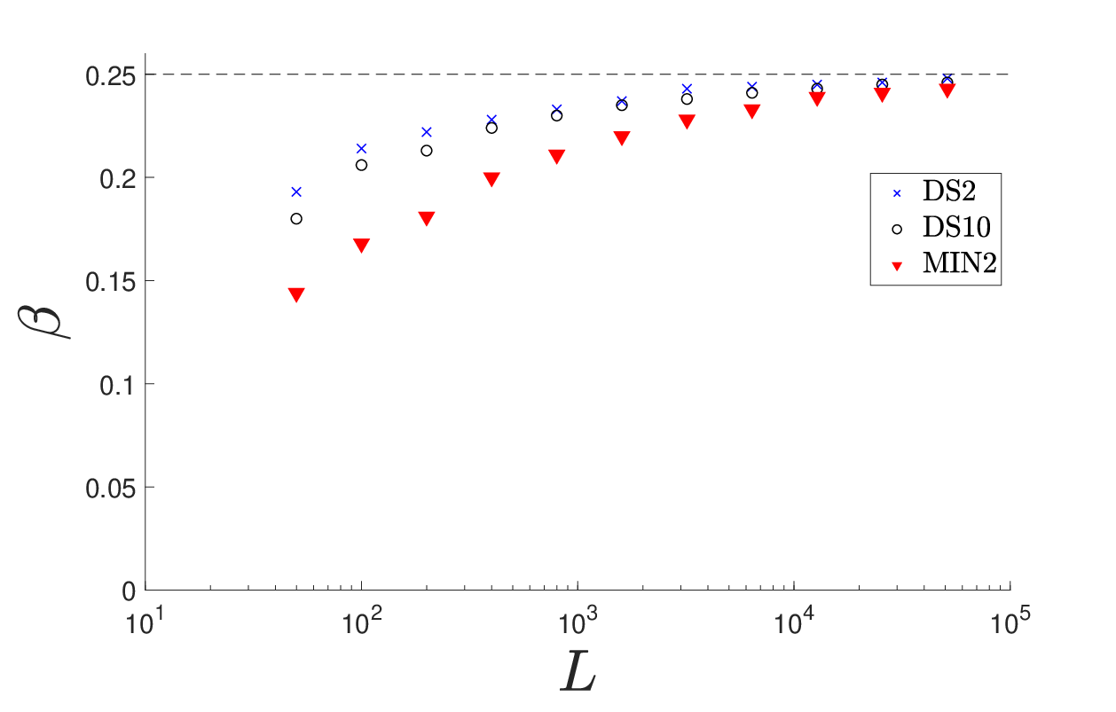
Finite size effects are not so important for the DF models where the model DF10 is only slightly different from the DF1 model, and it is practically equivalent to the model DFL (). This similarity among DF models can be understood from Fig. 6 which shows the frequency of downward hops of size for the DFL model.[18] According to Fig. 6, the frequency decreases exponentially, , making irrelevant the events for which is significantly larger than . Therefore, all DF models with are practically equivalent.
The minimum model has a completely different behavior with increasing because the deposited particles search for the lowest height site within a distance and the surface profile between the deposition site and the incorporation site is irrelevant. For any finite (more precisely, for any value of that does not scale with ), the minimum model belongs to the same Edwards-Wilkinson universality class, but simulations require increasingly larger and (and are therefore more computationally demanding) with increasing .

We now discuss the effect of the irrelevant quantities ( and the relaxation criterion) on the scaling function . The analytical expression for (see the Appendix) is
| (9a) | ||||
| (9b) | ||||
By using the analytical expression for and comparing it to the numerical profiles for the roughness obtained by the simulations, it is possible to extract and for each model[19] (see Table I). We then use these values to rescale the axes and obtain a single scaling curve for all models belonging to the EW universality class (see Fig. 7).
The noise appears to depend very weakly on the details of the relaxation process because its main source is the noise of the deposition process, which is the same in all simulations. The variability of reflects what we anticipated: relaxation is more effective for the MIN model and within the same model is more effective with increasing . As anticipated,
| (10) |
Finally, we expect that . As mentioned, if we use the numerical values of and from Table 1 to rescale the roughness, we obtain a single curve for all models as shown in Fig. 7.
| DF | ||
|---|---|---|
| MIN | ||
|---|---|---|

We see that is essentially independent of in both models and is almost constant for . The last question is how depends on . According to Table I, , which suggests the possible scaling . In Fig. 8 we test this assumption and find a good collapse for the curves at , 2, and 3.

V Conclusions
Our main goal has been to suggest that the kinetic roughening of deposition models can be studied by students with a limited physical and mathematical background, and that this topic can be a novel way to approach scaling and universality. We have also discussed how two relaxation models depend on , showing in particular that
- 1.
The minimum model has important finite size effects that are already visible for . These finite size effects are due to the fact that increases quadratically with , see Fig. 8.
- 2.
The downward funnelling model is well defined for increasing , because the probability of hops decays exponentially, as seen in Fig. 6.
We conclude by suggesting further directions that readers might desire to investigate.
- 1.
We propose to investigate the kinetic roughening process at the upper critical dimension of the Edwards-Wilkinson universality class, . In this case the roughness increases very slowly (logarithmically) and it might be necessary to investigate unusually large temporal and spatial scales to attain the scaling regime (we have not checked how large). We suggest using the rule with the least relaxation, that is, the DF1 model and with an initially flat surface, as in the simulations we have discussed. The statistical average over noise does not require special attention.
It may be of interest to point out a different “deposition with relaxation” model whose upper critical dimension is . [8, 20] The evolution of the surface is described by Eq. 14 with and scaling in is shown in Fig. 1 of Ref. [20]. Note the log-lin scale of the figure, which should also be used when studying the DF1 model for .
- 2.
In addition to the roughness, which is an average over noise, it would be interesting to study the distribution of the random variable . In a continuum picture we can replace Eq. (15) by Eq. (18), obtaining
(11) which shows that the height is a linear combination of independent random variables . According to the central limit theorem the distribution follows a Gaussian distribution with zero mean and standard deviation equal to the roughness . Is it possible to find numerically the distribution of (at fixed ) for the discrete model?
- 3.
Consider a deposition model for which right-left () symmetry has been broken, by introducing a probability in the DF models. If the relaxation process consists of reducing the height by hopping either to the right or to the left, we can break right-left symmetry by moving to the right with probability and to the left with probability . Modify the EW equation by adding the simplest term that breaks the symmetry without breaking all the other symmetries: up-down symmetry () and translation invariance in space () and time (). Show that a simple Galilean transformation leads back to the EW equation, without modifying the roughness exponent. Check this theoretical result numerically for the most asymmetric case ( or ).
*
Appendix A The Edwards-Wilkinson equation
In the following we sketch the derivation of the Edwards-Wilkinson equation for . For more details and for , see Ref. 12, Sec. 5.6.2.
Because of its linearity we can rewrite the Edwards-Wilkinson equation (5) as
| (12) |
We Fourier transform both sides and obtain
| (13) |
Equation (13) can be solved by multiplying both sides by and then integrating:
| (14) |
where . The first term on the right-hand side is related to the interface profile at and is negligible for large times. For simplicity we will assume an initial perfectly flat interface, , so that
| (15) |
By using the correlation of noise in Fourier space,
| (16a) | ||||
| (16b) | ||||
we find
| (17) |
We then use the inverse Fourier transform,
| (18) |
to find that the roughness becomes
| (19) | ||||
| (20) |
We make the change of variables and find
| (21) | ||||
|
where |
||||
| (22) | ||||
References
- [1] A.- L. Barabási and H. E. Stanley, Fractal Concepts in Surface Growth (Cambridge University Press, 1995).
- [2] P. Meakin, Fractals, Scaling and Growth Far from Equilibrium (Cambridge University Press, 1998).
- [3] A. Pimpinelli and J. Villain, Physics of Crystal Growth (Cambridge University Press, 1998).
- [4] L. M. Sander, “Diffusion-limited aggregation: a kinetic critical phenomenon?,” Contemporary Phys. 41, 203–218 (2000).
- [5] F. Family, “Scaling of rough surfaces: effects of surface diffusion,” J. Phys. A 19, L441–L446.
- [6] F. Family and T. Vicsek, “Scaling of the active zone in the Eden process on percolation networks and the ballistic deposition model,” J. Phys. A 18, L75–L81 (1985).
- [7] Dynamics of Fractal Surfaces, edited by F. Family and T. Vicsek (World Scientific, 1991).
- [8] J. Krug, “Origins of scale invariance in growth processes,” Adv. Phys. 46, 139–282 (1997).
- [9] C. Domb, The Critical Point: A Historical Introduction To The Modern Theory Of Critical Phenomena (Taylor & Francis, 1996).
- [10] B. Widom, “Scaling laws,” Scholarpedia 4 (10):9054 (2009), <www.scholarpedia.org/article/Scaling_laws>.
- [11] S. F. Edwards and D. R. Wilkinson, “The surface statistics of a granular aggregate,” Proc. R. Soc. London A 381, 17–31 (1982).
- [12] R. Livi and P. Politi, Nonequilibrium Statistical Physics: A Modern Perspective (Cambridge University Press, 2017).
- [13] See the following for a further comment about up-down symmetry in deposition models.
- [14] P. Meakin, P. Ramanlal, L. M. Sander, and R. C. Ball, “Ballistic deposition on surfaces,” Phys. Rev. A 34, 5091–5103 (1986).
- [15] J. M. Kim and J. M. Kosterlitz, “Growth in a restricted solid-on-solid model,” Phys. Rev. Lett. 62, 2289–2292 (1989).
- [16] M. Kardar, G. Parisi, and Y. C. Zhang, “Dynamic scaling of growing interfaces,” Phys. Rev. Lett. 56, 889–892 (1986).
- [17] K. Huang, Statistical Mechanics, 2nd ed. (Wiley, 1987).
- [18] Recall that is the deposition site and is the incorporation site. In the downward funnelling model the height of the interface decreases at each lattice site as is increased.
- [19] There have also been attempts to derive the growth equation from a continuum approximation of the Langevin equations for the discrete model, therefore allowing one to obtain an analytical expression for the parameters and for the Edwards-Wilkinson equation. However, this approach is more useful for relating atomistic processes to specific terms in the continuum equation rather than for obtaining reliable and functions. See, for example, D. D. Vvedensky, “Edwards-Wilkinson equation from lattice transition rules,” Phys. Rev. E 67, 025102(R) (2003).
- [20] J. Krug and P. Meakin, “Kinetic roughening of Laplacian fronts”, Phys. Rev. Lett. 66, 703-706 (1991).