Gravitational redshift in the void-galaxy cross-correlation function in redshift space
Abstract
We construct an analytic model for the void-galaxy cross-correlation function that enables theoretical predictions of the dipole signal produced dominantly by the gravitational redshift within voids for the first time. By extending a theoretical formulation for the redshift-space distortion of galaxies to include the second order terms of the galaxy peculiar velocity and the gravitational potential, we formulate the void-galaxy cross-correlation function multipoles in the redshift space, the monopole , dipole and quadrupole . We find that the dipole is dominated by the gravitational redshift, which provide a unique opportunity to detect the gravitational potential of voids. Thus, for the dipole , the gravitational redshift is crucial. Although the higher order effect is almost negligible on the monopole , it has an influence on the quadrupole . The effects from the random velocity of galaxies and the definition of the void center on the dipole signal are also discussed. Our model offers a new theoretical probe for the detection of gravitational redshift with voids and further tests on cosmology and gravity.
I Introduction
The large-scale structure of the Universe is observed in redshift maps of galaxy redshift surveys such as the Sloan Digital Sky Survey (SDSS). However, the mapping of galaxies from real space to redshift space produces statistical anisotropies caused by peculiar velocities relevant to the gravitational clustering, which is better known as the redshift-space distortion (RSD) [1, 2]. Recent galaxy redshift surveys enabled precise measurements of the RSDs in the galaxy map [3, 4, 5, 6, 7, 8, 9], which have been used to constrain important cosmological parameters, such as the linear growth rate of structure , useful for distinguishing between various cosmological models (e.g., [10, 11, 12]). Hence, the RSD in the large-scale structure of galaxies is beneficial when testing cosmological models, dark matter models, general relativity and its alternative theories such as modified gravity. Recently, general relativistic effects and higher order effects in the redshift map of galaxies have been investigated [14, 13, 15, 16, 17, 18, 19, 20, 21]. These works are extensions of precise modeling of galaxy distributions to include higher order effects of redshift-space distortions and other effects. The gravitational redshift and the second order Doppler effect (from the second order peculiar velocity) in the galaxy clusters are one of such topics [22, 23, 24, 25, 27, 26]. Measurements of the gravitational redshift with galaxies associated with clusters have been reported [22, 23, 24]. It is worth mentioning that recent research indicated that the gravitational redshift caused by the local gravitational potential may become a source of bias in the calibration of cosmological parameters using type Ia supernovae data combined with other cosmological probes, provided that we have no prior knowledge about the local gravitational potential [28]. This fact also addresses an importance for the investigation into the gravitational redshift on large scales.
The lowest density areas in the large-scale structure larger than Mpc, i.e., voids, which are one of the characteristic structures in the Universe, have become a useful tool for testing cosmological models and gravity theories [29, 30, 31, 32, 33, 34]. Precise modeling of voids with redshift-space distortions provides us with an approach for testing cosmological models. Accurate models of galaxy distributions of voids in the linear theory of density perturbations have been developed [35, 29, 36], and a constraint on the linear growth rate has been obtained by considering the RSD with voids [33]. The void-galaxy cross-correlation is utilized to compare galaxy distribution in redshift space inside and around voids with observations. The peculiar velocities of the galaxies are essential for void-galaxy cross-correlation in redshift space; however, these models are usually constructed up to the leading order of peculiar velocities of galaxies [36].
In this paper, we investigate possible signatures of the gravitational redshift and the higher order effect of peculiar velocities in the galaxy distribution associated with cosmic voids in redshift space, based on the progress of these previous works. We focus our analysis on void-galaxy cross-correlation, which represents the profile of the galaxy distribution of voids. We develop an analytic theoretical formulation for the void-galaxy cross-correlation function in redshift space including higher order effects of the second order terms of the galaxy peculiar velocity and the gravitational potential. Our model provides us with theoretical predictions for the multipoles of the void-galaxy cross-correlation function. In particular, we demonstrate that the dipole component reflects the gravitational redshift of a void structure for the first time. This aspect has been mostly neglected in previous works, which rely on the theory of the first order of the peculiar velocity.
This article is organized as follows. In Sec. II, we formulate the redshift space distortion up to the second order of the peculiar velocity and the gravitational potential. Then, we present an expression for the void-galaxy cross-correlation function in redshift space. The multipoles of the void-galaxy cross-correlation function are defined including the effects of the gravitational potential and the second order of the peculiar velocity of the spherical coherent motion of void, as well as random motions. In Sec. III, we adopt specific models for the density profile of a spherically symmetric void which allows us to demonstrate the multipoles of the void-galaxy cross-correlation function. In Sec. IV, we discuss the results and the physical reasons for the behavior of the multipoles of the void-galaxy cross-correlation function. We also discuss the nontrivial issue of how to choose the center of a void and its dependence on the results. Finally, we summarize our results and highlight our conclusions in Sec. V. We also briefly discuss prospective applications of our investigation for a comparison with observations. In Appendix A and B, we present complementary derivations of the mathematical formulas in Sec. II. In Appendix C we demonstrate the profiles of the density contrast, the velocity field, and the gravitational potential that we construct in Sec. III.2.
II Formulation
We will start with the formulation for the galaxy distribution in redshift space associated with a void, including the gravitational redshift and the second order of the peculiar velocity. We follow the theoretical formulation developed in Ref. [26] by beginning with a brief review of the formulation. When there is no effect from the gravitational potential and the peculiar velocity, the relation between the comoving distance and the redshift is given by
| (1) |
When there is a shift of the redshift from the gravitational potential and the peculiar velocity, , the distance in redshift space can be expressed as
| (2) |
where we evaluated the shift in the comoving distance by up to the second order.
To include the shift of a photon’s energy caused by the gravitational potential and the Doppler effect of peculiar velocity, we need to consider the second order terms of the peculiar velocity. We work within the Newtonian gauge of cosmological perturbation theory; however, the results will not depend on this choice because the void relevant to our problem is of the subhorizon scale. Denoting the gravitational potential and the peculiar velocity by and , respectively, we may express up to the order of [26],
| (3) |
where is the unit vector of the line of sight, and in Eq. (3) denotes the usual Doppler effect, while the term does the transverse Doppler effect. Inserting Eq. (3) into Eq. (2), we may write up to the order of as
| (4) |
For convenience, we assign our coordinate system by adopting the plane parallel approximation (distant observer approximation). Following this assumption, the coordinates perpendicular to the line-of-sight direction is the same, and the position of a galaxy in these directions takes the same value between the redshift space and the real space. However, the position parallel to the line-of-sight direction shifts, which is specified by Eq. (4). We adopt a coordinate system with its origin at the center of a void, and we denote the position of a galaxy as and , respectively, in the real space and the redshift space. We denote the comoving distance of the center of a void by , where is the redshift of the position of the center in the case, where there is no gravitational redshift effect or the Doppler effect.
As derived in the Appendix A, when the center of a void and the origin of the coordinate does not change between the real space and the redshift space, and are related by
| (5) |
where we introduced . It might be worth mentioning that the notations and are identical for the convenience of expression, as .
In the previous equation, we assumed that the center of a void assumes the same position in real space and redshift space. However, as we will discuss later, the definition of the center of a void is not a trivial problem. We may also consider the case that the center of a void is shifted in the redshift space, taking the gravitational redshift as . In this case, the center of the void is located at the distance , and the redshift space and the real space are related by
| (6) |
Note that Eq. (5) is reproduced by setting in Eq. (6). In the section below, we present the formulation with Eq. (6).
For convenience, we hereby adopt a convention in our derivation that the notation without a top arrow denotes the magnitude for an arbitrary vector . For instance, we have and . To formulate the void-galaxy cross-correlation in redshift space, we need to use the conservation property between redshift space and real space as follows:
| (7) |
where the superscript reminds us that is a quantity in redshift space. However, like all the quantities we will introduce in the following sections, this superscript can be omitted if we remember that these quantities as a function of redshift space separation , are defined in redshift space.
To obtain in Eq. (7), we need to express the physical space quantity and the transformation determinant using redshift-space quantities related to the separation within voids. We start by examining the terms in Eq. (6). To calculate the terms in the expression, we assume that the peculiar velocities of the galaxies associated with the void yield to the cosmological continuity equation as [29]
| (8) |
where the structure linear growth rate and the average density contrast of the void within the radius are involved. In Ref. [30], the authors tested the velocity profile in/around the voids in linear theory as Eq. (8) against numerical evaluation from simulation, and they found that Eq. (8), together with the best-fitted void profile, is consistent with simulation results, where the infall velocities corresponding to collapsing voids can be reproduced for smaller characteristic void radii. We will further address this issue subsequently when applying specific void profiles to test our results.
Since the peculiar velocity mainly contributes to RSDs along the line-of-sight direction , by defining , we have
where we defined
| (9) |
Here, we adopt the approximation since for a certain galaxy around the void, it is obvious that , where is negligible as a tiny quantity compared with the distance from distant observers. For further calculations, we need investigations into the relations for quantities and between real space and redshift space. To take the anisotropies related to line-of-sight direction into account, we define the dimensionless parameter , which is the cosine of the angle between and in redshift space. Then the components that are parallel to and perpendicular to are given as
| (10) |
respectively. On the other hand, the relation for parallel and perpendicular components between redshift space and real space can be written as
| (11) |
where denotes the shift on in the redshift coordinate along the line-of-sight direction caused by the redshift space distortions, i.e.,
| (12) |
Using Eqs. (6) and (II) we can express as a function of , such that
| (13) |
In the previous expression of , except for , all the other terms are of the order , which is supposed to be the same order of (see also Eq. (52)). This assumption is broadly used in the following derivations.
Since the leading term for is , it follows that terms up to the order of are sufficient to contain all terms; thus, we express up to the order of as
| (14) |
together with the direct transformation from Eq. (11),
| (15) |
Using Eqs. (14) and (15), and keeping terms up to the order of equivalent to , we write
| (16) |
where we use as a convention. Inserting Eqs. (14) and (16) into the expression for in Eq. (13), up to the order of , we finally have as the function of redshift quantities and as
| (17) | |||||
Thus, Eq. (15) with Eq. (17) give the complete relation between and , together with Eq. (10). Replacing with and using the relation , eventually we can calculate the coordinate transformation between physical space and redshift space as a function of the redshift-space quantities and as follows:
| (18) | |||||
On the other hand, using the relation Eq. (14), we can expand around for a small while still keeping terms up to as
Having calculated with respect to and in Eq. () and the determinant for coordinate transformation in Eq. (18), we eventually determine the redshift-space correlation function through the conservation property Eq. (7), as
| (20) | |||||
For more details of the derivation process from Eq. (4) to Eq. (20), please refer to Appendix A.
In Eq. (20) for , the anisotropies in redshift space associated with the line-of-sight direction are characterized by ; thus, the multipole components with respect to can be defined as
| (21) |
where are the Legendre polynomials. The monopole and quadrupole components can be written as
| (22) | |||||
| (23) | |||||
which is the generalization of the result by Ref. [36]. After dropping out terms in Eq. (23), the coefficients of our equation are different from those of Eq. (20) in Ref. [36] at first sight, but this is due to the difference of the definition of multipoles by a factor of . We now focus on the dipole component as follows:
| (24) |
We can see from the expressions related to the multipoles that the dipole includes the gravitational potential and , but the monopole and the quadrupole does not include terms concerning as well as . This fact suggests that only the dipole is influenced by the gravitational potential among the multipoles up to . The dipole is also influenced by the second order terms of the velocity; hence, it is reasonable to decompose the dipole into terms representing the contribution from the velocity component and the gravitational component as
| (25) |
where we defined
| (26) | |||
| (27) |
Furthermore, for convenience, we divide into two terms as
| (28) |
with
| (29) | |||
| (30) |
In the previous derivation, the velocity field is supposed to be a coherent field which follows from the linear theory of density perturbations. Random motions from the nonlinear effects, which causes the Fingers-of-God (FoG) effect could also be important. We may include the effect of the random velocities by following the Gaussian streaming model [36, 35]. This model remaps the galaxy distribution through a Gaussian random process with velocity dispersion . For simplicity, we adopt the following expression to take the random motions of galaxies with velocity dispersion into account for of Eq. (20)
| (31) |
with
| (32) |
where the upper index takes quantities with a random velocity into account, and the transformed quantity naturally contains the effect from the random velocity with the velocity dispersion .
With the aforementioned transformation, we can define the RSD multipoles with velocity dispersion similar to Eq. (21) as
| (33) |
For simplicity, the superscript in Eqs. (31) and (33) is omitted since it is well understood that our model for void RSD is constructed in redshift space.
| Parameter | Value | Remark |
|---|---|---|
| Overall redshift | ||
| Galaxy linear bias | ||
| Growth index for growth rate | ||
| Matter density parameter | ||
| Dark matter void central density | ||
| Void shape (steepness) parameter |
III Analysis on Specific Models for Void
In Sec. II, we have established the theoretical formulation for the void-galaxy cross-correlation function in redshift space and its multipoles, including the second order terms of the peculiar velocity as well as the gravitational potential. In this section, we demonstrate the behavior of the multipoles by adopting specific models for the void density profile.
III.1 A simple exponential model
To this end, we first adopt the simplest model of a spherical void density profile proposed in Ref. [33], which assumes the integrated density contrast of matter in the form
| (34) |
where , , and are the parameters; specifies the amplitude of the matter density contrast; is the characteristic radius of the void; and characterizes the steepness of the void wall. Here, recall that the we construct is the void-galaxy cross-correlation, where galaxies are biased tracers compared to dark matter. Hence, to evaluate the gravitational potential which is dominated by dark matter distribution, we need to include the galaxy bias in our model. In Ref. [37], the authors exhibited by simulation that the void-tracer cross-correlation, which in our case is just the void-galaxy cross-correlation, can be characterized by a linear relation. Hence, we simply assume a linear galaxy bias , which follows
| (35) |
where denotes the dark matter density contrast. In Ref. [37], for galaxies as tracers, is justified; thus, we adopt for simplicity. and are chosen to accord with the integrated galaxy density contrast proposed and presented in Ref. [33]. Here is related to the matter density contrast and the gravitational potential by the relation
| (36) | |||
| (37) |
where is the background matter density. Assuming a spatially flat cosmology with a cosmological constant, we may write , where is the matter density parameter and is the Hubble parameter at the present epoch. Then, the density contrast and the gravitational potential for the void are given by:
| (38) | |||
| (39) |
where is the incomplete gamma function.


By solving the continuity equation, the peculiar velocity of the radial direction can be written (see, e.g., Ref.[33]) as
| (40) |
where is the linear growth rate defined by the logarithmic differentiation with respect to the cosmological scale factor , which is approximately written as with and . We here assume that the coherent peculiar velocity of the galaxies follows Eq. (40).


Based on the modeling and parametrization above, we are now able to evaluate the void-galaxy cross-correlation function multipoles. Figures 2 and 2 plot the monopole component and the quadrupole component as functions of the dimensionless characteristic separation , in correspondence to Eq. (22) and Eq. (23). In each figure, the solid curve shows the result including the contribution from the terms up to , while the dashed curve shows the result for the terms up to . These two curves overlap in Figure 2, because the deviation is small. We show the difference for the monopole and quadrupole between and in the right panels of Figures 2 and 2, in which the correction due to terms for the monopole is , compared with the result. This suggests that the calculation up to is roughly sufficient to predict the monopole component and that the higher order terms slightly affect the prediction of the quadrupole component. The symbols in Figures 2 and 2 represent a plot of the case which includes the random velocity, Eq. (31). They demonstrate that the effect of the random motion is an important factor for the quadrupole component. The monopole and the quadrupole are irrelevant to the gravitational potential terms in our model; then, we next concentrate mainly on the analysis for the dipole signal.
Figure 4 plots the dipole component as a function of . The solid curve is the prediction without the random velocity, Eq. (24), while the symbols show the case including the contribution from the random velocity Eq. (31). For the dipole component, there is no contribution from the order of . Figure 4 compares the details of the dipole component. is the contribution from the second order terms of the velocity, and and are the contributions from the gravitational potential and the radial differentiation respectively, which are defined with Eqs. (28) and (25). This figure shows that is a minor contribution to the dipole and that the dipole is dominated by the contribution from the gravitational potential. Furthermore, this figure shows that arises from the terms and , which make contributions to the total result of the dipole at the same level.
III.2 A universal fitting model
Since the profile of Eq. (34) in Sec. III.1 combined with Eq. (8) cannot represent the infall velocities for smaller voids, we consider a best-fit universal void profile for more general cases. Following the formulation in Ref. [30], we can write the density contrast within the void as
| (41) |
where and are constants; and are some scale radius and characteristic void radius, respectively; and is the central density contrast, similar to Eq. (34). We define as the ratio of two parameters and . Then the integration within sphere radius leads to the integrated density contrast
| (42) | |||||
where is the hypergeometric function. In a similar way to Eq. (39), the gravitational potential characterized by the integrated density contrast Eq. (42) thus can be written as
| (43) | |||||
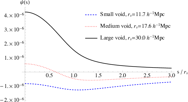
where is defined as , which is parameter dependent and can be determined from the boundary condition . Although analytic calculation for is difficult, we are able to evaluate it numerically when the parameters are specified for the void.
We choose three sets of parameters for the different typical size of voids, the large size void, the medium size void, and the small size void, which are listed in Table II, on the basis of the best-fit model in Ref. [30]. The profiles of the typical voids are presented in Appendix C in Figures 12 and 13, with Eqs. (41), (42), and (43) under the deliberate choice of parameters. The medium size void and the small size void model reproduce the behaviors of infall velocities presented by simulation in Ref. [30].
| Large | Medium | Small | Remark | |
|---|---|---|---|---|
| [Mpc] | ||||
| [Mpc2] |
Applying the void profiles to our formulation, we investigate the behaviors and the properties of the multipoles defined by Eqs. (21) and (33) in a similar way to what we have done in Sec. III.1. Figure 5 shows the results for the multipoles and Figure 6 shows the details of comparison for the dipole component in a similar way to Figures 2-4 and 4 in Sec. III.1. The profile of the model in the previous Sec. III.1 is similar to the large size void, so their multipoles’ behavior is almost the same. The multipoles of the medium size void and small size void are similar to the large size void; in particular, the dipole is dominated by the gravitational redshift for all three void sizes.


IV Discussions
In the previous section, we demonstrated how the higher order terms of the peculiar velocity and the gravitational potential influence the void-galaxy correlation functions through redshift space distortions. The higher order effect is not very significant for the monopole and the quadrupole components. However, the most interesting finding from the higher order effects is that the dipole component in the void-galaxy cross-correlation functions, dominantly reflects the gravitational potential through the gravitational redshift, as demonstrated in Figures 4 —6.
Photons from the central region of a large size void are blue-shifted compared with photons from the mean density region. This effect of the gravitational redshift is the origin of the dipole signal in the void-galaxy cross-correlation function. Most importantly, the dipole signal is therefore determined by the gravitational potential profile of the void. However, the dipole signal is not simply dominated by the gravitational potential . The contribution of the gravitational redshift to the dipole, Eq. (26), is given by the combination of the two terms,
| (44) |
namely, the terms from the gravitational potential and its gradient contribute equally to the dipole signal, as is demonstrated in Figures 4 and 6 .
Although we restrict ourselves to the predictions based on general relativity and discuss aspects of the robustness of our theoretical predictions, measurements of the gravitational potential provides a unique chance to test general relativity and other gravity theories. Moreover, these measurements may contribute to the clarification of bias on calibration of cosmological parameters due to local gravitational environments as mentioned previously. Theories kept in the linear regime for low-density regions associated with voids will make such tests less difficult compared with those which require nonlinear modeling of clustering of galaxies. To be a useful tool for testing gravity, the robustness of theoretical predictions is necessary. In Sec. III.1, we fixed the model parameters of a void (see Table I). Hence, it will be useful to check the robustness of our prediction of the results against the dependence on the model parameters in Table I.
In Figure 7, the dipole signal is plotted by fixing the velocity dispersion , by varying the set of parameters as ; ; ; and , based on the model of Eq. (34) in Sec. III A. We see that the dipole signal changes with the different values of , which characterizes the steepness of a void potential wall, and also the value of the redshift , which corresponds to different cosmological epoch. As the void potential becomes steeper, the gravitational potential takes a larger amplitude inside a void in the general case. In the cold dark matter model with a cosmological constant, the void gravitational potential decreases in proportion to . These properties explain the redshift dependence of the dipole in Figure 7. Nevertheless, our conclusions are not qualitatively altered by the choice of these parameters. Furthermore, our conclusion is robust against the change of model between Secs. III.1 and III.2.
We next consider the importance of the choice of the center of a void. In Figures 4 and 4, we showed the case in which the gravitational redshift of the center of a void is nonzero, i.e., the case . This is the case when the shift of the center of a void through the gravitational redshift is included as the extreme case. However, this term depends on the strategy employed to define the void center. For example, when the center of a void is determined using galaxies far from the central region, the position of the center is determined without the information , irrespective of the gravitational redshift of . In such a case, we should assume . Figure 8 compares the case with/without the term . These results indicate that the choice for the center of a void is not trivial for the dipole signal.
The void density contrast profile of Eq. (34) always generates a gravitational potential with a positive sign. However, the small size void and the medium size void of the best-fit profile in Ref. [30] in Sec. III.2 predict the gravitational potential with a negative sign, , as is demonstrated in Appendix C. This model allows us to test the case when the gravitational redshift from the center of the small and medium size voids may be redshifted rather than blueshifted. We further check the impact of the choice of the center of a void with the model in Sec. III.1, adopting the profile with the parameters in Table II for testing the robustness of our prediction. Figures 9, 10, and 11 show the impact of the choice of the void center on the dipole signal for the model in Sec. III.2. Figure 9 is the case of a large size void, which corresponds to the model in Sec. III.1, while Figures 10 and 11 are show the small size void and the medium size void.
For the small size void and the medium size void, the void potential possesses a global minimum at roughly rather than at infinity or at (), which is demonstrated in Figure 13 in Appendix C. In Figure 10, we plot the dipole signal for the small size void when the void center is sampled at the minimum of the gravitational potential at . In this case, the dipole signal becomes small though it is nonvanishing. In particular, the amplitude becomes even smaller when the random velocity is included. A more complicated situation occurs for the medium size void. The sign of the gravitational potential changes from the negative to positive in the interior region of the void (see Figure 13 in Appendix C). In this case could be either positive or negative. In Figure 11, we plot the dipole signal while adopting in a similar way to Figure 10. Thus the dipole signal depends on the choice of , though it is nonvanishing.
The choice of the void center depends on the algorithm used in data analysis. We need to investigate the behavior of the dipole signal by adopting the realistic algorithm for finding the center of a void with mock catalogs of galaxies from numerical simulations. Although this is beyond the scope of the present paper, we briefly discuss this problem. In a realistic analysis of void-finding algorithms, there are two algorithms best suited to define the center of a void. One is the lowest-density center, which is determined as the center of the lowest density galaxy in a void and its three most adjacent neighboring galaxies [38, 39]. This algorithm is equivalent to finding the largest empty sphere that can be found within the void. Another is the volume-weighted barycenter which is mainly used for irregular-shaped voids (Ref. [39]). Roughly, the first definition of the center by the minimum density center corresponds to the case including as the maximum, while the second volume-weighted barycenter might correspond to the case without . This is because should be included when the center of a void is determined by the information about the central region, while should not be included when the center is determined by the information about the outskirt region of a void.
In a realistic situation, each void is not spherically symmetric, and statistical errors should be included in identifying the center of the void as well as . To consider such an effect, we may be able to consider a probability distribution function for it in a similar way to Eq. (31) as
| (45) |
where stands for the void-galaxy cross-correlation with consideration of the probability distribution on the term. However, the probability distribution function of , i.e., may be highly model dependent and deviate from the Gaussian distribution. So we would rather leave this part to more sophisticated consideration in the future.
Finally in this section, we discuss the influence of spherical averaging or stacking of the void profile on the dipole signal. In Refs. [40, 41], the authors argued that the conventional way of spherical stacking of void may lead to a stacked profile with steeper central density contrast and milder transition to the high-density ridge at the void boundary compared with the actual situation. In Ref. [41], the authors introduced a boundary profile closer to the actual individual void obtained by stacking over distances of volume elements from the void boundary rather than spherical averaging over its center, which has a flat core with a sharp transition to the high-density ridge at the void boundary. This is very similar to the profile of Eq. (34) in Sec. III.1 with a very large value of .
We find that the gravitational potential of a profile similar to Ref. [41] is flatter than that of the spherically stacked profile and almost zero at the exterior regions of the void. If the void center is determined with a profile like this by tracers at the exterior regions of the void, for example, at , will be closer to zero than that with the spherically stacked profile. This result suggests that the influence of the choice of void center characterized by will be smaller if we sample the voids using tracers from exterior regions by the method in Ref. [41]. Methods like this could make the dipole signal less sensitive to the choice of void center. Thus, the strategy to choose the void center changes the dipole signal, which causes some difficulty in the comparison of our results with observations, although the monopole and the quadrupole do not depend on this choice.
V Summary and Conclusion
In this paper, we have presented an analytic model for the void-galaxy cross-correlation function in redshift space including the higher order terms of the peculiar velocity and the gravitational potential through redshift space distortions. By adopting specific models for a void density profile, including a universal best-fit profile which can produce infall velocities in the linear regime of density perturbations, we have quantitatively demonstrated the influence of the higher order terms on the multipole components of the void-galaxy cross-correlation. In particular, we have found that the dipole signal dominantly reflects the gravitational potential through the gravitational redshift. Our conclusion is qualitatively robust against the change of the model parameters and the void profiles. However, we have also discussed the possible dependence of the dipole signal on the algorithm for determining the center of a void. This dependence should be investigated with the use of numerical simulations with mock catalogs by adopting a practical algorithm to determine the center of a void, including other systematic errors. The idea of consideration for the probability distribution function of the term may be helpful, but this is left as a future investigation. However, in principle, our finding presents the possibility of a new approach to direct measurements of the gravitational potential of voids.
In Ref. [29], the monopole and the quadrupole multipoles of the void-galaxy cross-correlation function were measured with the SDSS III LOWZ sample and the CMASS sample. Our formulation may serve as an extension to the analytic theory for quantitative analysis on these measurements with higher order accuracy. The error bars of the multipoles are quite small; thus, we may detect the dipole component in future analysis. Such an analysis would help in the understanding of voids and provide a test for general relativity and cosmological models in combination with observations using other methods, e.g., measurement of the thermal Sunyaev-Zel’dovich effect around voids and the weak lensing measurements of voids [42].
Acknowledgments.— This work is supported by MEXT/JSPS KAKENHI Grants No. 15H05895, No. 17K05444, and No. 17H06359 (K. Y.). We thank A. Taruya, S. Saito, and D. Parkinson for useful communications during the workshop YITP-T-17-03. We thank an anonymous referee for helpful comments, which improved the manuscript.
References
- [1] N. Kaiser, Mon. Not. R. Astron. Soc. 227, 1 (1987).
- [2] A. J. S. Hamilton, arXiv:astro-ph/9708102.
- [3] J. A. Peacock, Nature (London) 410, 169 (2001).
- [4] L. Guzzo et al., Nature (London) 451, 541 (2008).
- [5] K. Yamamoto, G. Huetsi, T. Sato, Prog. Theor. Phys 120, 609 (2008).
- [6] F. Beutler, C. Blake, M. Colless, D. H. Jones, L. Staveley-Smith, G. B. Poole, L. Campbell, Q. Parker, W. Saunders, and F. Watson, Mon. Not. Roy. Astron. Soc., 423, 3430 (2012).
- [7] F. Beutler et al., Mon. Not. Roy. Astron. Soc., 443, 1065 (2014).
- [8] H. Gil-Marin et al., Mon. Not. Roy. Astron. Soc. 460, 4188 (2016).
- [9] R. Rugerri et al., arXiv:1801.02891.
- [10] K. Yamamoto, G. Nakamura, G. Huetsi, T. Narikawa, T. Sato, Phys. Rev. D 81, 103517 (2010).
- [11] F. G. Mohammad, S. de la Torre, D. Bianchi, L. Guzzo, and J. A. Peacock, Mon. Not. R. Astron. Soc. 458, 1948 (2016).
- [12] A. De Felice, S. Mukohyama, Phys. Rev. Lett. 118, 091104 (2017).
- [13] N. Bartolo, D. Bertacca, M. Bruni, K. Koyama, R. Maartens, S. Matarrese, M. Sasaki, L. Verde, and D. Wands, Phys. Dark Universe 13, 30 (2016).
- [14] A. Raccanelli, D. Bertacca, D. Jeong, M. C. Neyrinck, A. S. Szalay, Phys. Dark Universe 19, 109 (2018).
- [15] A. Raccanelli, F. Montanari, D. Bertacca, O. Dore, R. Durrer, J. Cosmol. Astropart. Phys. 05 (2016) 009.
- [16] D. Bertacca, A. Raccanelli, N. Bartolo, M. Liguori, S. Matarrese, L. Verde, Phys. Rev. D 97, 023531 (2018).
- [17] J. Yoo, Class. Quant. Grav. 31 234001 (2014).
- [18] J. Yoo, A. L. Fitzpatrick, M. Zaldarriaga, Phys. Rev. D 80, 083514 (2009).
- [19] S. Alam, H. Zhu, R. A. C. Croft, S. Ho, E. Giusarma, and D. P. Schneider, Mon. Not. R. Astron. Soc. 470, 2822 (2017).
- [20] H. Zhu, S. Alam, R. A. C. Croft, S. Ho and E. Giusarma, Mon. Not. R. Astron. Soc. 471, 2345 (2017).
- [21] M.-A., Breton, Y. Rasera, A. Taruya, O. Lacombe, S. Saga, arXiv:1803.04294.
- [22] R. Wojtak, S. H. Hansen, J. Hjorth, Nature (London) 477, 567 (2011).
- [23] H. S. Zhao, J. A. Peacock, B. Li, Phys. Rev. D 88, 043013 (2013).
- [24] P. Jimeno, T. Broadhust, J. Coupon, K. Umetsu, R. Lazkov, Mon. Not. R. Astron. Soc. 448, 1999 (2015).
- [25] N. Kaiser, Mon. Not. R. Astron. Soc. 435, 1278 (2013).
- [26] D. Sakuma, A. Terukina, K. Yamamoto, C. Hikage, Phys. Rev. D 97, 063512 (2018).
- [27] Y.-C. Cai, N. Kaiser, S. Cole, C. Frenk, Mon. Not. R. Astron. Soc. 468 1981 (2017).
- [28] R. Wojtak, T. M. Davis, J. Wiis, J. Cosmol. Astropart. Phys. 07 (2015) 025.
- [29] N. Hamaus, M.-C. Cousinou, A. Pisani, M. Aubert, S. Escoffier, and J. Weller, J. Cosmol. Astropart. Phys. 07 (2017) 014.
- [30] N. Hamaus, P. M. Sutter, and B. D. Wandelt, Phys. Rev. Lett. 112, 251302 (2014).
- [31] Q. Mao, A. A. Berlind, R. J. Scherrer, M. C. Neyrinck, R. Scoccimarro, J. L. Tinker, C. K. McBride, and D. P. Schneider, Astrophys. J. 835, 160 (2017).
- [32] D. Micheletti et al., Astron. Astrophys. 570, A106 (2014).
- [33] A. J. Hawken et al., Astron. Astrophys. 607, A54 (2017).
- [34] Y.-C. Cai, N. Padilla, and B. Li, Mon. Not. R. Astron. Soc. 451, 1036 (2015).
- [35] Y.-C. Cai, A. Tayolor, J. A. Peacock, and N. Padilla, Mon. Not. R. Astron. Soc. 462, 2465 (2016).
- [36] S. Nadathur and W. Percival, arXiv:1712.07575.
- [37] G. Pollina, N. Hamaus, K. Dolag, J. Weller, M. Baldi, and L. Moscardini, Mon. Not. R. Astron. Soc. 469, 787 (2017).
- [38] S. Nadathur, S. Hotchkis, and R. Crittenden, Mon. Not. R. Astron. Soc. 467, 4067 (2017).
- [39] S. Nadathur, Mon. Not. Roy. Astron. Soc. 461, 358 (2016).
- [40] R. Wojtak, D. Powell, and T. Abel, Mon. Not. R. Astron. Soc. 458, 4431 (2016).
- [41] M. Cautun, Y.-C. Cai, and C. S. Frenk, Mon. Not. R. Astron. Soc. 457, 2540 (2016).
- [42] D. Alonso, J. C. Hill, R. Hlozek, and D. N. Spergel, Phys. Rev. D 97, 063514 (2018).
Appendix A Complementary Derivations for Eq. (20)
We will present some details for derivations in Sec. II. Since we adopted the plane parallel approximation, we will assign the three-dimensional coordinates and in redshift space and real space, respectively, as
| (46) |
where is the coordinate perpendicular to the line-of-sight direction. Denoting the position of the center of a void as and in real space and the redshift space, respectively we have
| (47) |
from Eq. (4), where we adopted the coordinate system with its origin at the center of a void and in the real space and the redshift space, respectively.
When we choose , we have
| (48) |
Introducing the conformal Hubble parameter and using the relation will slightly simplify the verbose expression as Eq. (5) that can be expressed as
| (49) |
This is for the case of the center of a void and the origin of the coordinate does not change between the real space and the redshift space.
When we choose , we have
| (50) |
This is for the case when the center of the void and the origin of the coordinate shift from the real space to the redshift space.
Note that Eq. (49) is reproduced by setting in Eq. (50). Then we present the formulation with Eq. (50) in the following section.
Then the component parallel to in Eq. (6) is in fact
| (51) |
Comparing this with the first line of Eq. (11), where , we get Eq. (12) for .
Substituting the dimensionless quantity that we defined in Eq. (9) into Eq. (12), we write Eq. (13) as
In in the previous derivation, all terms are terms except ; thus, we can write
| (52) |
which will be convenient in later derivations.
As an example of how we keep terms up to the order of , we now consider the term which frequently appears in the expression for as Eq. (13). Remembering Eq. (52) will be very helpful in the process of keeping terms up to the order of in the following section.
Using Eq. (14) for and Eq. (15) for repeatedly, together with Eq. (52), we write
| (53) | |||||
In the above expression, noticing Eq. (52) again, we further write for the second term in the expression above
| (54) | |||||
Also, for the third term in Eq. (53), using the definition for in Eq. (10), transforming similarly to Eq. (53) will lead to
| (55) | |||||
Inserting Eqs. (54) and (55) back into Eq. (53) will lead us to Eq. (16).
With in Eq. (14)and in Eq. (16) calculated up to the order of , we can now rewrite following the same previous procedure as Eq. (13), which is a function of the redshift-space quantities and as Eq. (17). Notice that , hence we have directly.
Eq. (15) and Eq. (17) give the complete relation between and , so we can write
| (56) | |||||
It is also obvious that
| (57) |
On the other hand, relation given as
| (58) | |||||
simply leads to Eq. ().
Appendix B Potentially Useful Quantities
From Eq. (20), it might also be noted that for , which stands for the direction perpendicular to the line-of-sight direction, we have
| (59) | |||||
The cosine angle between the galaxy displacement vector from the void center and the line-of-sight in real space is
| (60) | |||||
Appendix C Void Profiles Constructed from Ref.[30]
We present the density profiles (Figure 12) and the velocity profile and the gravitational potential (Figure 13) constructed from the model in Ref. [30]. Here we adopt the three typical sizes of voids, the large size void, the medium size void, and the small size void, whose parameters are listed in Table II. These three models correspond to those adopted in the text of the present paper.