Bunching-antibunching crossover in harmonically trapped few-body Bose-Fermi mixtures

The Hamiltonian of our 1D harmonically trapped ultracold Bose-Fermi mixture is given by $\hat{H}=\hat{H}_{b}+\hat{H}_{f}+\hat{H}_{bf}$, where

and $\textit{h}_{\sigma}(x_{\sigma})=-\frac{\hbar^{2}}{2m_{\sigma}}\frac{\partial^{2}}{\partial x_{\sigma}^{2}}+\frac{1}{2}m_{\sigma}\omega^{2}x_{\sigma}^{2}$ is the single-particle Hamiltonian for the harmonic confinement of the $\sigma=b(f)$ species. $\hat{\psi}_{\sigma}^{\dagger}(x_{\sigma})$ [$\hat{\psi}_{\sigma}(x_{\sigma})$] is the field operator that creates (annihilates) a $\sigma$-species particle at position $x_{\sigma}$. For simplicity, we consider here equal trapping frequencies for both species. Moreover, we assume that the Bose-Bose (intraspecies) as well as the Bose-Fermi (interspecies) interactions are of zero range and can be modeled by contact potentials of strengths [68, 58]

Here $a_{b}$ ($a_{bf}$) is the 3D Bose-Bose (Bose-Fermi) $s$-wave scattering length and $C\approx 1.4603$ is a constant. The parameters $a_{\bot,b}=\sqrt{2\hbar/m_{b}\omega_{\bot}}$ and $a_{\bot,bf}=\sqrt{\hbar/\mu\omega_{\bot}}$ describe the transverse confinement, with $\mu=m_{b}m_{f}/({m_{b}+m_{f}})$ being the reduced mass and we assume the transverse trapping frequency $\omega_{\bot}$ to be equal for both species. Moreover, we focus on the repulsive interaction regime, i.e., $g_{b}$ $(g_{bf})\geqslant 0$. It should be pointed out that, due to the Pauli-exclusion principle, the $s$-wave contributions to the fermionic scattering vanish and, hence, (spin-polarized) fermions become noninteracting at low collision energies. In the following discussion, we rescale the Hamiltonian (1) for the units of the energy and length with $\eta=\hbar\omega$ and $\xi=\sqrt{\hbar/m_{b}\omega}$, respectively. We explore a mixture made of two fermions and two bosons, i.e., $N_{f}=N_{b}=2$ and investigate the ground-state properties in both the mass-balanced ($\beta=1$) and the mass-imbalanced ($\beta=5,25$) regimes, with $\beta=m_{f}/m_{b}$ being the mass ratio. Let us note that such a 1D mixture is experimentally accessible by imposing strong transverse and weak longitudinal confinement for a binary mixture made of ${}^{7}\textrm{Li}$-${}^{6}\textrm{Li}$ ($\beta\approx 1$) [10, 11], ${}^{171}\textrm{Yb}$-${}^{39}\textrm{K}$, ${}^{40}\textrm{K}$-${}^{7}\textrm{Li}$ ($\beta\approx 5$) or ${}^{171}\textrm{Yb}$-${}^{7}\textrm{Li}$ ($\beta\approx 25$). Moreover, the contact interaction strengths can be controlled experimentally by tuning the $s$-wave scattering lengths via Feshbach or confinement-induced resonances [68, 69, 70].

In order to explore our few-body system described by $\hat{H}$ from first principles, we employ the very recently developed ML-MCTDHX method [63, 64, 65]. Its efficient wave function representation scheme allows one to compute eigenstates as well as the temporal evolution of a many-body system including all correlations.

To this end, the state of the 1D Bose-Fermi mixture $|\Psi(t)\rangle$ is first expanded as $|\Psi(t)\rangle=\sum_{i,j=1}^{M}A_{ij}(t)|\psi_{i}^{f}(t)\rangle|\psi_{j}^{b}(t)\rangle$, with $\{|\psi_{i}^{\sigma}(t)\rangle\}_{i=1}^{i=M}$ being the states for $\sigma$ species, which form a set of orthonormal functions. It is important to note that both the coefficients $A_{ij}(t)$ and the species states $\{|\psi_{i}^{\sigma}(t)\rangle\}$ are time dependent. Furthermore, each species state $|\psi_{i}^{\sigma}(t)\rangle$ is expressed as linear combinations of the number states according to $|\psi_{i}^{\sigma}(t)\rangle=\sum_{\textbf{n}|N_{\sigma}}C_{i,\textbf{n}}^{\sigma}(t)|\textbf{n}\rangle^{\sigma}_{t}$, where $|\textbf{n}\rangle_{t}^{\sigma}=|n_{\sigma 1},n_{\sigma 2},\cdots\rangle$ are the number states for the $\sigma$ species under the constraint of particle number conservation $\sum_{i}n_{\sigma i}=N_{\sigma}$. Moreover, these number states $|\textbf{n}\rangle_{t}^{\sigma}$ are built by time-dependent single-particle functions (SPFs) $\{|\phi_{k}^{\sigma}(t)\rangle\}_{k=1}^{s_{\sigma}}$. Using the Lagrangian variational principle results in the coupled integro-differential equations of motion for both coefficients $A_{ij}(t)$ and $C_{i,\textbf{n}}^{\sigma}(t)$ as well as the SPFs $|\phi_{k}^{\sigma}(t)\rangle$, which allows us to obtain the variationally optimized SPFs $|\phi_{k}^{\sigma}(t)\rangle$ and accordingly the state $|\Psi(t)\rangle$.

Finally, we note that the numbers $s_{\sigma}$ and $M$ are the main control parameters for the numerical simulations, in which $s_{\sigma}$ truncates the dimension of the single-particle Hilbert space, leading to individual species spaces of size $K_{\sigma}=\left(\begin{array}[]{c}N_{\sigma}+s_{\sigma}-1\\ s_{\sigma}-1\end{array}\right)\left[K_{\sigma}=\left(\begin{array}[]{c}s_{\sigma}\\ N_{\sigma}\end{array}\right)\right]$ for $N_{\sigma}$ bosons (fermions). The value of $M\leqslant\text{min}\{K_{A},K_{B}\}$ defines how many species states are used to construct the full many-body Hilbert space.

A particular feature which we observed for our mixture is the bunching-antibunching crossover for the bosonic species, which occurs as a function of the inter- and the intraspecies interaction strengths. Indeed, for a fixed $g_{bf}$ one detects a bunching to antibunching transition by increasing $g_{b}$ (cf. Fig. 1), while for a fixed $g_{b}$ one finds the reverse transition for increasing $g_{bf}$ (cf. Fig. 2). In order to visualize this crossover, we introduce the reduced two-body density for the bosonic species

The physical meaning of $\rho^{b}_{2}(x_{1},x_{2})$ is the probability of finding one boson at position $x_{1}$ while the second one is at $x_{2}$, which naturally describes the spatial correlations between two bosons. Experimentally the spatial profile of the reduced two-body density can be measured via in situ absorption imaging (see [71] and references therein).

As an exemplary case, we elaborate how the bosonic species undergoes a transition from bunching to antibunching for fixed $g_{bf}=2.0$ and increasing $g_{b}$. The reduced two-body densities are depicted in Fig. 1 for the mass-imbalanced case of $\beta=5$, together with the corresponding reduced one-body densities $\rho^{b}_{1}(x)=\int\rho_{2}^{b}(x,x^{\prime})dx^{\prime}$. Let us note that during the transition the two fermions are localized at the trap center due to the large mass ratio (see below). For the case $g_{b}=0$, we observe that the bosons are bunching at either the left or right side of the trap, represented by the two dominant peaks around $x_{1}=x_{2}\approx\pm 1$ in the reduced two-body density. With increasing $g_{b}$, the bunching becomes energetically unfavorable, which immediately ramps down (up) the density in the vicinity of the diagonal ($x_{1}=x_{2}$) [off-diagonal ($x_{1}=-x_{2}$)] regions [cf. Fig. 1(b)]. Finally, for the case $g_{b}=2.0$, the bosons completely anti-bunch such that each boson resides on one side of the trap. Let us highlight that the reduced one-body density fails to capture the above crossover. For increasing $g_{b}$, we observe only a slight change of $\rho^{b}_{1}(x)$ with a minor broadening of the density distribution owing to the increment of the bosonic repulsion [cf. Fig. 1(d)]. Since $\rho^{b}_{1}(x)$ is obtained by the partial trace of one particle over the corresponding reduced two-body density, which inevitably loses the two-particle correlations. Complementarily, the transition of the antibunching to the bunching behavior with the increase of $g_{bf}$ is presented as well (cf. Fig. 2). For increasing $g_{bf}$ and fixed $g_{b}$, we observe that the reduced two-body density evolves from the original profile with dominant populations on the off diagonal to the case of dominant populations on the diagonal. Similarly, this transition is not captured by the corresponding reduced one-body density as well, resulting in a deep dent of the density distribution from the original Gaussian profile with increasing the Bose-Fermi repulsion [cf. Fig. 2(d)].

In order to quantify the degree of the bosonic bunching (antibunching), we introduce the two-body density imbalance as $\textit{P}=P_{s}-P_{d}$, where

with $P_{s}(P_{d})$ being the probability of finding two bosons at the same side (different sides) of the trap. Thereby the two-body density imbalance directly reveals the probability difference between these two situations. Here, the prefactor $2$ originates from the parity symmetry of the Hamiltonian $\hat{H}$. Importantly, based on the observations for the spatial profiles of the bosonic reduced two-body densities, we arrive at the criteria of bosonic bunching (antibunching) as $\textit{P}>0$ ($\textit{P}<0$). Moreover, due to the normalization condition: $\int dx_{1}dx_{2}~\rho^{b}_{2}(x_{1},x_{2})=1$, the two-body density imbalance takes values within the interval $[-1,1]$.

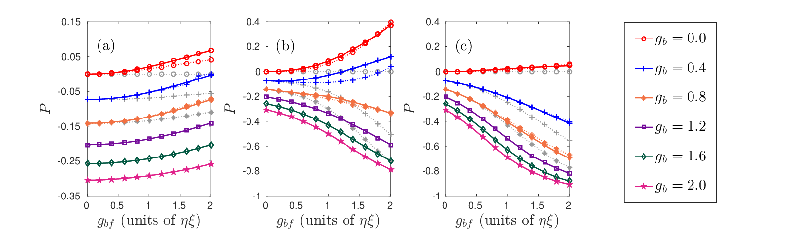
In Figs. 3(a)–3(c), we present the two-body density imbalance $P$ as a function of $g_{bf}$ for a set of discrete values of $g_{b}$ and various fixed values of $\beta$ (colored solid lines). Note, here, that the presented results are obtained from the ab initio ML-MCTDHX simulations, which differ from the results using the adopted approximations and effective descriptions (see below). As expected, the increase of $g_{b}$ always reduces the $P$ value since the bosonic repulsion favors antibunching. However, the situation becomes more complicated once additionally $g_{bf}$ and $\beta$ are varied. For the equal-mass case, we observe that the increase of $g_{bf}$ leads to a monotonous increase of the $P$ value, whereas, in the mass-imbalanced regimes, an increase or decrease of the $P$ value depending on the value of $g_{b}$ being below or above a critical value $g_{b}^{c}$ takes place [cf. Figs. 3(b) and 3(c)]. Interestingly, the $g_{b}^{c}$ decreases for increasing mass ratio, from $g_{b}^{c}\approx 0.6$ for $\beta=5$ to $g_{b}^{c}\approx 0.2$ for $\beta=25$. Besides, the mass ratio has also a significant impact on the absolute range of $P$ values with $P\in(-0.3,0.1)$ for $\beta=1$, while, becoming $P\in(-0.8,0.4)$ and $P\in(-0.9,0.1)$ for $\beta=5$ and $25$, respectively.

Before closing this section, let us briefly discuss the spatial profiles of the reduced one-body density $\rho^{\sigma}_{1}(x)$, which denotes the probability of finding a $\sigma$-species particle at position $x$. In Fig. 4, we present $\rho^{\sigma}_{1}(x)$ for both species for changing $g_{bf}$ and $\beta$ and $g_{b}=0$. Despite the fact that $\rho^{\sigma}_{1}(x)$ depends on the value of $g_{b}$ as well, we observe the increase of $g_{b}$ ($g_{b}\in[0,2]$) only slightly affects these density profiles, resulting in a minor broadening of the bosonic density distribution owing to the increment of the bosonic repulsion (results are not shown here). For increasing $\beta$, we find the fermionic density distribution shrinks dramatically while the bosonic one is less affected. This observation can be quantitatively understood via the harmonic confinement encoded in the length scale $l_{\sigma}=\sqrt{\hbar/m_{\sigma}\omega}$ [58]. A mass difference leads to different confinement lengths with the relative ratio $l_{b}/l_{f}=\sqrt{\beta}$, and thereby results in a smaller spatial overlap of the density profiles. By contrast, the increase of $g_{bf}$ has a large impact on both species, resulting in stronger demixing or phase separation of the two species.

In order to elucidate the origin of the above-analyzed bunching-antibunching crossover, hereafter, we present effective theoretical descriptions based on the fact that mixture is weakly entangled (see below). The ground-state wave function of the 1D Bose-Fermi mixture can be written in the form

according to the Schmidt decomposition [72], where $\lambda_{i}$ are the Schmidt numbers with descending order, i.e., $\lambda_{1}>\lambda_{2}>\cdots$, which are real positive numbers and obey the constraint $\sum_{i}\lambda_{i}=1$ due to the normalization of the wave function $|\Psi\rangle$. Here $|\psi_{i}^{\sigma}\rangle$ denotes the $i$th Schmidt state for species $\sigma$. In addition, all the Schmidt states $\{|\psi_{i}^{\sigma}\rangle\}$ form an orthonormal basis. We emphasize that the Schmidt numbers directly reveal the interspecies correlations as $S=-\sum_{i}\lambda_{i}\text{log}_{2}\lambda_{i}$, with $S$ being the entanglement entropy [72]. Moreover, the case $\lambda_{1}=1$, i.e., $\lambda_{i\neq 1}=0$, results in $S=0$, indicating that the mixture is nonentangled.

In order to quantitatively evaluate the interspecies correlations, we introduce the species depletion as $\kappa=1-\lambda_{1}$, and depict it as a function of both $g_{b}$ and $g_{bf}$ for various fixed mass ratios (cf. Fig. 5). Albeit the fact that the increase of $g_{bf}$ always ramps up the species depletion, however, the $\kappa$ value is also affected by both $g_{b}$ and $\beta$. For instance, for a fixed $g_{bf}$, the increase of $g_{b}$ significantly decreases the $\kappa$ value for $\beta=5,25$, while it has minor impact on the case where the atoms possess the same mass, leaving the $\kappa$ value more or less unchanged. On the other hand, for fixed interaction strengths, the mass ratio can lead to dramatic variations of the species depletion. For the cases $g_{b}=0$ and $g_{bf}=2.0$, the $\kappa$ value is $0.134$ ($\beta=5$), $0.047$ ($\beta=1$), and $0.024$ ($\beta=25$). Finally, we stress that the investigated Bose-Fermi mixture essentially remains within the weak entanglement regime ($\kappa\ll 1$); here about $100\%$, $86\%$, and $100\%$ of the parameter space for $\beta=1,5,$ and $25$, respectively, exhibit a species depletion below $\kappa=0.05$. It is this fact that we can exploit in the following to obtain an effective theoretical description for the bosonic species accounting for the bunching-antibunching crossover.

The above effective descriptions introduce significant insights in the study of mixtures while, at the same time, enable us to explore the physics effectively present in a single species. This is why we have been able to see that the effective potential in the strong mass-imbalanced regimes becomes a double well [cf. Figs. 6(g)–6(i)], which offers the opportunity to map the effective Hamiltonian for the bosonic species to a lattice model. In order to elucidate this lattice model, we focus on the situation for $\beta=25$ in the following discussions. Furthermore, in Figs. 6(g)–6(i), we clearly see that the presence of a central barrier induces the formation of bands with a small energy spacing $\delta\epsilon$ between the two lowest single-particle eigenstates. Importantly, a large gap to the next band severely suppresses particle excitations to the higher bands. In this way, the bosons mainly populate the lowest band. With this knowledge, we adopt the single-band approximation and obtain the Hamiltonian for the two-site extended Bose-Hubbard (EBH) model for the two bosons as (for a corresponding derivation please see the Appendix)

where $\hat{a}^{\dagger}_{R/L}$ ($\hat{a}_{R/L}$) denote the creation (annihilation) operators for the right or left site and the coefficients $J$, $U$, and $V$ represent the hopping amplitude and the on-site interaction, as well as the nearest-neighbor interaction, respectively. Compared to the conventional Bose-Hubbard model, the EBH model possesses richer phases including the density-wave phases and the Haldane insulator phase, in addition to the superfluid and the Mott insulating phase [75, 76].

Before proceeding, it is instructive to note that the discussions on the two-site EBH model as well as the computed coefficients are in the framework of the beyond SMF description. Let us first briefly comment on the roles of both $g_{b}$ and $g_{bf}$ with respect to the above two-site EBH model. The role of $g_{b}$ is relatively simple since the increment of the bosonic repulsion mainly increases the on-site repulsion, resulting in the increase of the $U$ value. In comparison, the role of $g_{bf}$ is more complicated. On one hand, the increase of $g_{bf}$ leads to a rapid increase of the height of the central barrier which, in turn, leads to a monotonous decrease of the hopping amplitude $J$. On the other hand, it also increases the strength of the induced interaction resulting in an increase of the on-site attraction, as well as the off-site repulsion.

The computed coefficients for the two-site EBH model are presented in Fig. 8. As anticipated, the increase of $g_{bf}$ leads to a decrease of the hopping amplitude $J$ since the increment of the lattice depth severely suppresses the particle hopping between the two sites. In contrast, the coefficients of both on-site and nearest-neighbor interactions are defined by the interplay between the induced interaction and the bosonic contact repulsion. For the case $g_{b}=0$ [cf. Fig. 8(a)], the induced interaction creates attractive on-site and repulsive nearest-neighbor interactions due to the long-range behavior of the spatial profile [cf. Fig. 7(c)]. Importantly, the on-site attraction combined with a weak hopping amplitude facilitates the “cat-state-like” phase [77], with the wave function $|\Psi\rangle=1/\sqrt{2}~(|2,0\rangle+|0,2\rangle)$, which corresponds to the bosonic bunching. Here $|N_{L},N_{R}\rangle=1/\sqrt{N_{L}!\,N_{R}!}(\hat{a}_{L}^{\dagger})^{N_{L}}(\hat{a}_{R}^{\dagger})^{N_{R}}|vac\rangle$, with $N_{L(R)}$ being the particle number of the left (right) site under the constraint of particle conservation $N_{L}+N_{R}=2$. In contrast, for the cases with a large bosonic repulsion [cf. Fig. 8(b)], the on-site repulsion dominates and, in turn, supports the formation of a “Mott-state-like” phase, which corresponds to the antibunching of the bosons. As a result, the above two-site EBH model supports a transition from the cat-state-like phase to the Mott-state-like phase, which coincides with the bunching-antibunching crossover of the more general binary mixture system investigated above.

In order to quantitatively judge the validity of the two-site EBH model, we inspect the corresponding two-body density imbalance

denoting the probability difference between finding two bosons on the same site and finding them on different sites. Moreover, the ground state $|\Psi_{\text{EBH}}\rangle$ is obtained by diagonalizing the Hamiltonian $\hat{H}_{\text{EBH}}$ in the space spanned by the basis $\{|2,0\rangle,|1,1\rangle,|0,2\rangle\}$. In Fig. 9(a), we present the computed $P_{\text{EBH}}$ for $g_{b}=0.0,0.4,0.8$ (red dashed lines). As compared to the results obtained from the ab initio ML-MCTDHX simulations (blue solid lines), the $P_{\text{EBH}}$ values possess only minor discrepancies. Importantly, using the two-site EBH model one can even quantitatively capture the critical bosonic repulsion $g_{b}^{c}$ that we discussed before, which manifests its applicability. Meanwhile, we also clearly see that the obtained lattice model successfully accounts for the transition from bunching to antibunching with increasing bosonic repulsion [cf. Fig. 9(b)].

References

- [1] W. D. Phillips, Rev. Mod. Phys. 70, 721 (1998); I. Bloch, J. Dalibard, and W. Zwerger, Rev. Mod. Phys. 80, 885 (2008).
- [2] M. Greiner, O. Mandel, T. Esslinger, T. W. Hänsch, and I. Bloch, Nature (London) 415, 39 (2002).
- [3] I. B. Spielman, W. D. Phillips, and J. V. Porto, Phys. Rev. Lett. 98, 080404 (2007).
- [4] T. Stöferle, H. Moritz, C. Schori, M. Köhl, and T. Esslinger, Phys. Rev. Lett. 92, 130403 (2004).
- [5] S. B. Papp, J. M. Pino, and C. E. Wieman, Phys. Rev. Lett. 101, 040402 (2008).
- [6] S. Tojo, Y. Taguchi, Y. Masuyama, T. Hayashi, H. Saito, and T. Hirano, Phys. Rev. A 82, 033609 (2010).
- [7] D. J. McCarron, H. W. Cho, D. L. Jenkin, M. P. Köppinger, and S. L. Cornish, Phys. Rev. A 84, 011603(R) (2011).
- [8] J. Catani, L. De Sarlo, G. Barontini, F. Minardi, and M. Inguscio, Phys. Rev. A 77, 011603(R) (2008).
- [9] D. S. Hall, M. R. Matthews, J. R. Ensher, C. E. Wieman, and E. A. Cornell, Phys. Rev. Lett. 81, 1539 (1998).
- [10] A. G. Truscott, K. E. Strecker, W. I. McAlexander, G. B. Partridge, and R. G. Hulet, Science 291, 2570 (2001).
- [11] F. Schreck, L. Khaykovich, K. L. Corwin, G. Ferrari, T. Bourdel, J. Cubizolles, and C. Salomon, Phys. Rev. Lett. 87, 080403 (2001).
- [12] Z. Hadzibabic, C. A. Stan, K. Dieckmann, S. Gupta, M. W. Zwierlein, A. Görlitz, and W. Ketterle, Phys. Rev. Lett. 88, 160401 (2002).
- [13] G. Roati, F. Riboli, G. Modugno, and M. Inguscio, Phys. Rev. Lett. 89, 150403 (2002).
- [14] G. Modugno, G. Roati, F. Riboli, F. Ferlaino, R. J. Brecha, and M. Inguscio, Science 297, 2240 (2002).
- [15] K. Günter, T. Stöferle, H. Moritz, M. Köhl, and T. Esslinger, Phys. Rev. Lett. 96, 180402 (2006).
- [16] M. W. Zwierlein, A. Schirotzek, C. H. Schunck, and W. Ketterle, Science 311, 492 (2006).
- [17] B. DeMarco and D. S. Jin, Science 285, 1703 (1999).
- [18] K. M. O’Hara, S. L. Hemmer, M. E. Gehm, S. R. Granade, and J. E. Thomas, Science 298, 2179 (2002).
- [19] C. A. Regal, M. Greiner, and D. S. Jin, Phys. Rev. Lett. 92, 040403 (2004).
- [20] M. W. Zwierlein, C. A. Stan, C. H. Schunck, S. M. F. Raupach, A. J. Kerman, and W. Ketterle, Phys. Rev. Lett. 92, 120403 (2004).
- [21] K. Mølmer, Phys. Rev. Lett. 80, 1804 (1998).
- [22] L. Viverit, C. J. Pethick, and H. Smith, Phys. Rev. A 61, 053605 (2000).
- [23] N. Nygaard and K. Mølmer, Phys. Rev. A 59, 2974 (1999).
- [24] X. X. Yi and C. P. Sun, Phys. Rev. A 64, 043608 (2001).
- [25] H. Pu and N. P. Bigelow, Phys. Rev. Lett. 80, 1130 (1998).
- [26] Tin-Lun Ho and V. B. Shenoy, Phys. Rev. Lett. 77, 3276 (1996).
- [27] A-Hai Chen and Gao Xianlong, Phys. Rev. A 86, 065602 (2012).
- [28] Gao Xianlong, Phys. Rev. A 87, 023628 (2013).
- [29] R. Roth and H. Feldmeier, Phys. Rev. A 65, 021603(R) (2002).
- [30] T. Miyakawa, T. Suzuki, and H. Yabu, Phys. Rev. A 64, 033611 (2001).
- [31] X. J. Liu, M. Modugno, and H. Hu, Phys. Rev. A 68, 053605 (2003).
- [32] N. P. Robins, W. Zhang, E. A. Ostrovskaya, and Y. S. Kivshar, Phys. Rev. A 64, 021601(R) (2001).
- [33] S. K. Yip, Phys. Rev. A 64, 023609 (2001).
- [34] H. Pu, W.P. Zhang, M. Wilkens, and P. Meystre, Phys. Rev. Lett. 88, 070408 (2002).
- [35] X. J. Liu and H. Hu, Phys. Rev. A 67, 023613 (2003).
- [36] C. J. Pethick and H. Smith, Bose-Einstein Condensation in Dilute Gases (Cambridge University Press, New York, 2008).
- [37] L. P. Pitaevskii and S. Stringari, Bose-Einstein Condensation and Superfluidity (Oxford University Press, New York, 2016).
- [38] M. Gaudin, Phys. Lett. A 24, 55 (1967).
- [39] C. N. Yang, Phys. Rev. Lett. 19, 1312 (1967).
- [40] M. D. Girardeau and A. Minguzzi, Phys. Rev. Lett. 99, 230402 (2007).
- [41] M. D. Girardeau and M. Olshanii, Phys. Rev. A 70, 023608 (2004).
- [42] M. A. Cazalilla and A. F. Ho, Phys. Rev. Lett. 91, 150403 (2003).
- [43] L. Mathey, D.-W. Wang, W. Hofstetter, M. D. Lukin, and Eugene Demler, Phys. Rev. Lett. 93, 120404 (2004).
- [44] T. Giamarchi, Quantum Physics in One Dimension, (Clarendon Press, Oxford, 2004).
- [45] A. N. Wenz, G. Zürn, S. Murmann, I. Brouzos, T. Lompe, S. Jochim, Science 342, 457 (2013).
- [46] G. Zürn, A. N. Wenz, S. Murmann, A. Bergschneider, T. Lompe, and S. Jochim, Phys. Rev. Lett. 111, 175302 (2013).
- [47] S. Murmann, A. Bergschneider, V. M. Klinkhamer, G. Zürn, T. Lompe, S. Jochim, Phys. Rev. Lett. 114, 080402 (2015).
- [48] F. Serwane, G. Zürn, T. Lompe, T. B. Ottenstein, A. N. Wenz, and S. Jochim, Science 332, 336 (2011).
- [49] G. Zürn, F. Serwane, T. Lompe, A. N. Wenz, M. G. Ries, J. E. Bohn, and S. Jochim, Phys. Rev. Lett. 108, 075303 (2012).
- [50] S. Murmann, F. Deuretzbacher, G. Zürn, J. Bjerlin, S. M. Reimann, L. Santos, T. Lompe, and S. Jochim, Phys. Rev. Lett. 115, 215301 (2015).
- [51] A. S. Dehkharghani, F. F. Bellotti, and N. T. Zinner, J. Phys. B: At., Mol., Opt. Phys. 50 144002 (2017).
- [52] H. P. Hu, L. Pan, and S. Chen, Phys. Rev. A 93, 033636 (2016).
- [53] A. S. Dehkharghani, A. G. Volosniev, and N. T. Zinner, J. Phys. B: At., Mol., Opt. Phys. 49 085301 (2016).
- [54] D. Pȩcak, A. S. Dehkharghani, N. T. Zinner, and T. Sowiński, Phys. Rev. A 95, 053632 (2017).
- [55] K. Keiler, S Krönke and P. Schmelcher, New J. Phys. 20 033030 (2018).
- [56] P. Siegl, S. I. Mistakidis and P. Schmelcher, arXiv:1803.07881 (2018).
- [57] M. Pyzh, S Krönke, C. Weitenberg and P. Schmelcher, New J. Phys. 20 015006 (2018).
- [58] A. C. Pflanzer, S. Zöllner, and P. Schmelcher, Phys. Rev. A 81, 023612 (2010).
- [59] A. C. Pflanzer, S. Zöllner, and P. Schmelcher, J. Phys. B: At., Mol., Opt. Phys. 42 231002 (2009).
- [60] H. P. Hu, L. M. Guan, and S. Chen, New J. Phys. 18, 025009 (2016).
- [61] B. Fang, P. Vignolo, M. Gattobigio, C. Miniatura, and A. Minguzzi, Phys. Rev. A 84, 023626 (2011).
- [62] F. Deuretzbacher, D. Becker, J. Bjerlin, S. M. Reimann, and L. Santos, Phys. Rev. A 95, 043630 (2017).
- [63] L. Cao, V. Bolsinger, S. I. Mistakidis, G. M. Koutentakis, S. Krönke, J. M. Schurer and P. Schmelcher, J. Chem. Phys. 147, 044106 (2017).
- [64] L. Cao, S. Krönke, O. Vendrell, and P. Schmelcher, J. Chem. Phys. 139, 134103 (2013).
- [65] S. Krönke, L. Cao, O. Vendrell, and P. Schmelcher, New J. Phys. 15, 063018 (2013).
- [66] H.-D. Meyer, U. Manthe, and L. Cederbaum, Chem. Phys. Lett. 165, 73 (1990).
- [67] J. Chen, J. M. Schurer, and P. Schmelcher, Phys. Rev. Lett. 121, 043401 (2008).
- [68] M. Olshanii, Phys. Rev. Lett. 81, 938 (1998).
- [69] C. Chin, R. Grimm, P. Julienne, and E. Tiesinga, Rev. Mod. Phys. 82 1225 (2010).
- [70] T. Köhler, K. Góral, and P. S. Julienne, Rev. Mod. Phys. 78 1311 (2006).
- [71] C. L. Hung, C. Chin, arXiv:1312.0498 (2014).
- [72] A. Pathak, Elements of Quantum Computation and Quantum Communication, (Taylor & Francis, 2013).
- [73] M. J. Bijlsma, B. A. Heringa, and H. T. C. Stoof, Phys. Rev. A 61, 053601 (2000).
- [74] J. J. Kinnunen, G. M. Bruun, Phys. Rev. A 91, 041605(R) (2015).
- [75] T. D. Kühner, S. R. White, and H. Monien, Phys. Rev. B 61, 12474 (2000).
- [76] D. Rossini and R. Fazio, New J. Phys. 14 065012 (2012).
- [77] M. Ueda, Fundamentals and New Frontiers of Bose-Einstein Condensation (World Scientific, Singapore, 2010).