Elasticity as the basis of allostery in DNA

When a ligand binds to DNA it induces conformational changes at the binding site which could propagate to regions tens of base-pairs away, thereby encouraging or inhibiting the binding of a second ligand in those places. Such interactions between two binding agents are called allosteric interactions. Our focus here is on a mechanism for allostery based on elasticity of long molecules. Although we will illustrate our theory using DNA as an example, long range allosteric interactions have been documented in actin, microtubules and helical peptide chains. For example, myosin binds to actin filaments leading to suppression of the formation of cofilin clusters via allosteric signalling [11]. Long range structural changes induced by taxol binding to microtubules inside a cell prevents cell division thus making it a potent anti-tumor agent [9]. The transfer of chiral stimulus triggered by a binding agent across a helical peptide chain gives the molecule an overall chiral character and is yet another instance of allostery [12]. We will analyze allostery in dsDNA because detailed experimental and simulation results are available for it [1, 5, 7], thus allowing quantitative comparisons with our theory.
DNA comprises of two helical strands held together via complementary base-pairing. When a ligand, such as a protein or a drug, binds to DNA it exerts forces and moments on the double helix [2, 14] causing deformations at the base-pair level. We use the theory of birods [10] to investigate these deformations. A birod consists of two elastic strands which interact through an elastic web. This construction makes it suitable for investigating the deformations at the base-pair level in a DNA molecule which a homogeneous rod model cannot capture [8]. The latter ignores the double helical structure and the elasticity of the base pairs, both of which are crucial to the problem under consideration.

In this letter, $(\cdot)_{x}$ denotes $\frac{\partial{(\cdot)}}{\partial{x}}$. Lower case letters such as $a,r,\beta^{\pm}$ are scalars, bold lower case letters such as $\mathbf{t}^{+},\mathbf{b}^{-}$ are vectors while bold upper case letters such as $\mathbf{R}^{-},\mathbf{R}^{+}_{0},\mathbf{Z}$ are $3\times 3$ tensors.
We assume the phosphate backbones comprising of phosphodiester bonds to be inextensible and unshearable elastic strands. Since these backbones consist of consecutive single bonds which allow for free rotation about the bond, we assume that they can not resist twisting moments. The base pairing is represented by the elastic web which is capable of extending, shearing, bending and twisting. In addition to the elastic energy, we consider contributions from the stacking energy which is associated with the change in orientations of the successive base pairs.
We denote the helical strands as $\pm$; their positions in the reference state are denoted by $\mathbf{r}^{\pm}_{0}$. We use arclength parameter $x$ to parametrize the double helix. Thus,

$$\begin{split}\mathbf{r}^{+}_{0}&=a(\cos\omega x\penalty\ \mathbf{e}_{1}+\sin\omega x\penalty\ \mathbf{e}_{2})+x\penalty\ \mathbf{e}_{3},\\ \mathbf{r}^{-}_{0}&=a(\cos(\omega x+\alpha)\penalty\ \mathbf{e}_{1}+\sin(\omega x+\alpha)\penalty\ \mathbf{e}_{2})+x\penalty\ \mathbf{e}_{3},\end{split}$$

(1)

where $a=1$ nm is the radius of the DNA helix, $p=3.4$ nm is the pitch, $\omega=\frac{2\pi}{p}$ and $\alpha$ is the phase difference between the helices. Here we assume $\alpha=\pi$ to make the computations analytically tractable. We consider a deformed configuration where the double helix extends and twists about $\penalty\ \mathbf{e}_{3}$, and its radius and phase angle also change due to binding of ligands. The deformed state of the $\pm$ strands is denoted by $\mathbf{r}^{\pm}(x)$, where

$$\begin{split}&\mathbf{r}^{+}(x)=(a+r)\Big(\cos(\omega x+\beta^{+})\penalty\ \mathbf{d}_{1}+\sin(\omega x+\beta^{+})\penalty\ \mathbf{d}_{2}\Big)+(x+\int_{-\infty}^{x}a\xi^{+}dx)\penalty\ \mathbf{e}_{3},\\ &\mathbf{r}^{-}(x)=-(a+r)\Big(\cos(\omega x+\beta^{-})\penalty\ \mathbf{d}_{1}+\sin(\omega x+\beta^{-})\penalty\ \mathbf{d}_{2}\Big)+(x+\int_{-\infty}^{x}a\xi^{-}dx)\penalty\ \mathbf{e}_{3},\end{split}$$

(2)

such that $\penalty\ \mathbf{d}_{1x}=k_{3}\penalty\ \mathbf{d}_{2}$ and $\penalty\ \mathbf{d}_{2x}=-k_{3}\penalty\ \mathbf{d}_{1}$. We assume all the displacement and strain parameters $r,\beta^{\pm}$ and $\xi^{\pm}$ vanish at $x=\pm\infty$ because the deformations caused by the proteins are local. The change in radius $r$, change in the phase angle $\beta^{\pm}$, stretch $\xi$, and the twist $k_{3}$ are assumed to be small ($\sim O(\varepsilon)$) such that second order terms such as $r^{2}$ and $\xi\beta^{-}$ are negligible. However, there could be finite rotations resulting from $k_{3}$.
We need to solve the balance equations for a birod [10], which are

$$\begin{split}&\textbf{{n}}^{\pm}_{x}\mp\textbf{{f}}+\textbf{{l}}=0,\\ &\textbf{{m}}^{\pm}_{x}+\mathbf{r}^{\pm}_{x}\times\textbf{{n}}^{\pm}+\frac{1}{2}(\mathbf{r}^{+}-\mathbf{r}^{-})\times\textbf{{f}}\mp\textbf{{c}}+\textbf{{h}}=0,\end{split}$$

(3)

where $\textbf{{m}}^{\pm}$ and $\textbf{{n}}^{\pm}$ are the contact moment and contact force respectively in $\pm$ strands. f and c are the distributed force and distributed moment exerted by the $+$ strand on the $-$ strand. l and h are the body force and body moment exerted by the base pairs onto both $\pm$ strands. We use the position vectors for the deformed helix $\mathbf{r}^{\pm}(x)$ (eqn. 2) to compute these quantities.
The outer strands are inextensible which means $|\mathbf{r}_{x}^{\pm}|=|\mathbf{r}_{0x}^{\pm}|$ yielding,

$$\begin{split}\omega^{2}r+a\omega(k_{3}+\beta^{\pm}_{x})+\xi^{\pm}=0.\end{split}$$

(4)

We use the above equation to eliminate $\xi^{\pm}$. We attach a director frame $\mathbf{R}^{\pm}=[\textbf{n}^{\pm}_{0}\quad\textbf{b}^{\pm}_{0}\quad\textbf{t}^{\pm}_{0}]$ to each cross-section of the $\pm$ strands, where $\textbf{n}^{\pm}_{0}$, $\textbf{b}^{\pm}_{0}$, and $\textbf{t}^{\pm}_{0}$ are the normal, binormal, and tangent in the reference state to $\pm$ strand, respectively. $\textbf{n}^{\pm},\textbf{b}^{\pm}_{0},\textbf{t}^{\pm}_{0}$ and the curvature in the reference configuration $\Omega^{\pm}_{0}(=\omega\sin k)$ are computed using eqn. 1 (see the supplement). Similarly, we use eqn.2 to compute the the Frenet-Serret frame $\mathbf{R}^{\pm}=[\textbf{n}^{\pm}\quad\textbf{b}^{\pm}\quad\textbf{t}^{\pm}]$ and curvature $\Omega^{\pm}$ in the deformed state. We neglect terms higher than first order such as $r\beta^{+},\xi^{-}r\sim O(\varepsilon^{2})$ and summarize the results in eqn. 5. The bending moment in the outer strands $\textbf{{m}}^{\pm}$ is proportional to the change in curvature $\kappa^{\pm}=\Omega^{\pm}-\Omega_{0}^{\pm}$ and is directed along the binormal $\textbf{b}^{\pm}$ such that $\textbf{{m}}^{\pm}=EI\kappa^{\pm}\textbf{b}^{\pm}$ where $EI$ is the bending modulus of the strand. Note that the twisting moment is zero.

$$\begin{split}&\Omega^{\pm}=\Omega^{\pm}_{0}-(r_{xx}+\xi^{\pm})\cos k+(\beta^{\pm}_{x}+k_{3})\sin k,\\ &\mathbf{R}^{\pm}=[\textbf{n}^{\pm}\quad\textbf{b}^{\pm}\quad\textbf{t}^{\pm}]=\mathbf{Z}\mathbf{R}^{\pm}_{0}(\mathbf{1}+\Theta^{\pm}),\\ &\mathbf{Z}=\penalty\ \mathbf{d}_{1}\otimes\penalty\ \mathbf{e}_{1}+\penalty\ \mathbf{d}_{2}\otimes\penalty\ \mathbf{e}_{2}+\penalty\ \mathbf{e}_{3}\otimes\penalty\ \mathbf{e}_{3},\\ &\Theta^{\pm}=\begin{bmatrix}0&-\theta^{\pm}_{3}&\theta^{\pm}_{2}\\ \theta^{\pm}_{3}&0&-\theta^{\pm}_{1}\\ -\theta^{\pm}_{2}&\theta^{\pm}_{1}&0\end{bmatrix}\end{split}$$

(5)

		$\displaystyle\theta^{\pm}_{1}=r\omega+a(\beta^{\pm}_{x}+k_{3}),\quad\theta^{\pm}_{2}=-r_{x}\cos k+\beta^{\pm}\sin k,$
		$\displaystyle\theta^{\pm}_{3}=\frac{-\omega r_{x}-a(\beta^{\pm}_{xx}+k_{3x})}{\omega\sin k}-\frac{(r_{x}\cos k-\beta^{\pm}\sin k)\cos k}{\sin k}.$

Now, we compute the bending and twisting of the web which represents base-pairing. We attach a director frame $\mathbf{Q}_{0}$ to both $+$ and $-$ end of the base pair (fig.1).

$$\begin{split}\mathbf{Q}_{0}=[\penalty\ \mathbf{e}_{r}\quad\penalty\ \mathbf{e}_{\theta}\quad\penalty\ \mathbf{e}_{3}],\end{split}$$

(6)

where $\penalty\ \mathbf{e}_{r}=\cos\omega x\penalty\ \mathbf{e}_{1}+\sin\omega x\penalty\ \mathbf{e}_{2}$ and $\penalty\ \mathbf{e}_{\theta}=-\sin\omega x\penalty\ \mathbf{e}_{1}+\cos\omega x\penalty\ \mathbf{e}_{2}$. As the birod deforms, these frames respectively get mapped to $\mathbf{Q}^{\pm}$. We compute $\mathbf{Q}^{\pm}$ using the deformation of $\mathbf{R}^{\pm}$ from eqn. (5).

$$\begin{split}\mathbf{Q}^{\pm}=\mathbf{Z}\mathbf{R}_{0}^{\pm}(\textbf{I}+\Theta^{\pm})\mathbf{R}_{0}^{\pm T}\mathbf{Q}_{0},\quad\quad\Theta^{\pm}\sim O(\varepsilon).\end{split}$$

(7)

Now, we can compute the rigid rotation $\mathbf{Q}$ and micro-rotation $\mathbf{P}$ for each base pair. The micro-rotation contains information about the ‘difference’ between the rotations $\mathbf{Q}^{\pm}$. This is related to the moment transferred by the base pair c via an elastic constitutive relation for the web,

$$\begin{split}&\mathbf{P}=(\mathbf{Q}^{+}\mathbf{Q}^{-T})^{\frac{1}{2}}=\mathbf{Z}(\textbf{I}+\Phi^{c})\mathbf{Z}^{T}.\end{split}$$

(8)

Here, $\Phi^{c}=\frac{\mathbf{R}^{+}\Theta^{+}\mathbf{R}^{+T}-\mathbf{R}^{-}\Theta^{-}\mathbf{R}^{-T}}{2}$ is a skew symmetric tensor. The moment transferred by the base pair is directly proportional to the Gibbs vector of $\mathbf{P}$. $\boldsymbol{\eta}=\tan\frac{\lambda}{2}\mathbf{\hat{k}}$ is a Gibbs rotation vector for a rotation matrix T if $\textbf{T}\mathbf{\hat{k}}=\mathbf{\hat{k}}$ and $1+2\cos\lambda=$ trT. In our case, the Gibbs vector of $\mathbf{P}$ is $2\boldsymbol{\eta}=2\mathbf{Z}\bar{\boldsymbol{\eta}}=\mathbf{Z}\mathbf{\boldsymbol{\phi^{c}}}$, where $\mathbf{\phi^{c}}$ is the axial vector of skew symmetric tensor ${\Phi^{c}}$. Note that in the reference state, $\boldsymbol{\eta}_{0}=0$ since $\mathbf{P}_{0}=(\mathbf{Q}_{0}\mathbf{Q}_{0}^{T})^{1/2}=\mathbf{I}$. The rigid rotation of the base pair $\mathbf{Q}=\mathbf{P}\mathbf{Q}^{-}$. Here

$$\begin{split}&\mathbf{Q}=\mathbf{Z}(1+\Phi)\mathbf{Q}_{0},\end{split}$$

(9)

and $\Phi=\frac{\mathbf{R}^{+}\Theta^{+}\mathbf{R}^{+T}+\mathbf{R}^{-}\Theta^{-}\mathbf{R}^{-T}}{2}$ is a skew symmetric matrix. The moment exterted by $+$ strand on the $-$ strand by means of the elastic web, c, is computed using $\textbf{{c}}=\mathbf{Q}\mathbf{H}\mathbf{Q}^{T}\boldsymbol{\eta}$ where $\mathbf{H}=$ diag$[H_{1},\penalty\ H_{2},\penalty\ H_{3}]$ are the elastic moduli. Now, we shift our focus to the extension and shear of the web. In the reference configuration the displacement between the two strands $\mathbf{w}_{0}=\frac{\mathbf{r}^{+}_{0}-\mathbf{r}^{-}_{0}}{2}=a\penalty\ \mathbf{e}_{r}$. In the deformed configuration $\mathbf{w}=\frac{\mathbf{r}^{+}-\mathbf{r}^{-}}{2}$. The force f exerted by $+$ strand on the $-$ strand is computed using $\textbf{{f}}=\mathbf{Q}\mathbf{L}(\mathbf{Q}^{T}\mathbf{w}-\mathbf{Q}_{0}^{T}\mathbf{w}_{0})$ where $\mathbf{L}=$ diag$[L_{1},\penalty\ L_{2},\penalty\ L_{3}]$ are the elastic moduli. Complete expressions for f and c are provided in the supplement.
We now consider the contributions from the stacking energy. The center line of the double helix $\penalty\ \mathbf{e}_{3}$ undergoes both twist $k_{3}$ and extension $\xi=\frac{\xi^{+}+\xi^{-}}{2}$. We associate a quadratic stacking energy $E_{s}=K_{c}k_{3}^{2}+K_{e}(\frac{\xi^{+}+\xi^{-}}{2})^{2}$ to penalize this change in the orientation of successive base pairs. Due to this energy, the base pairs exert a body force l and a body moment h on both $\pm$ strands which are given by

$$\begin{split}\textbf{{l}}=K_{e}(\frac{\xi^{+}+\xi^{-}}{2})\penalty\ \mathbf{e}_{3},\quad\quad\textbf{{h}}=K_{c}k_{3}\penalty\ \mathbf{e}_{3}.\end{split}$$

(10)

Now we have all the ingredients for solving the governing differential equations of a birod. Substituting these quantities in the balance laws (eqn.3) gives us a set of 12 differential equations. The complete procedure for solving those equations is in the supplement, however we highlight crucial points here. It follows from the governing equations that $\beta^{+}=\beta^{-}(=\beta$ say), $n^{c}_{3}=n_{1}=n_{2}=0$. $\beta^{+}=\beta^{-}$ implies $\xi^{+}=\xi^{-}=(\xi$ say) thereby reducing 12 equations to 6 equations in 6 unknowns $r,\beta,k_{3},n^{c}_{1,2},n_{3}$. We look for solutions of the form,

$$\begin{split}&r(x)=r_{0}e^{-\lambda x},\beta(x)=\beta_{0}e^{-\lambda x},\penalty\ \xi(x)=\xi_{0}e^{-\lambda x},\\ &n^{c}_{1}(x)=n^{c}_{10}e^{-\lambda x},\penalty\ n^{c}_{2}(x)=n^{c}_{20}e^{-\lambda x},\penalty\ n_{3}(x)=n_{30}e^{-\lambda x}.\end{split}$$

(11)

We substitute this form into the governing equations (eqn. 3) and obtain an eigenvalue problem in $\lambda$. In order to make further progress, we need the values of the elastic constants. We use $K_{c}=80$ pNnm², $K_{e}=600$ pN, $L_{1}=L_{2}=L_{3}=H_{1}=H_{2}=H_{3}=10$ pN. In the supplement, we show that these values yield the correct twist, stretch and twist-stretch coupling moduli for double stranded B-DNA. Solving for the eigenvalues $\lambda$ we get

$$\begin{split}\lambda=\pm\zeta\pm i\omega,\quad\quad\zeta=0.32\text{nm}^{-1},\end{split}$$

(12)

and the solution for the strain parameters $y_{1}=r,y_{2}=k_{3}$ and $y_{3}=\beta$ is of the form:

$$\begin{split}y_{i}(x)=&A_{1}\mathbf{V}_{1}(i)e^{(-\zeta-i\omega)x}+A_{2}\mathbf{V}_{2}(i)e^{(-\zeta+i\omega)x}+B_{1}\mathbf{V}_{3}(i)e^{(\zeta-i\omega)x}+B_{2}\mathbf{V}_{4}(i)e^{(\zeta+i\omega)x}.\end{split}$$

(13)

where $\mathbf{V}_{j}(i)$ is the $i^{th}$ component of the eigenvector corresponding to the eigenvalue in the exponent. Clearly, the decay length $\zeta$ is only a function of the elastic parameters of dsDNA, in agreement with the conclusion of Kim et al [5]. Note that the strain parameters are exponentially decaying while oscillating with the period $\omega$ of the double helix. We impose the boundary conditions on $r$ and $\beta$ remembering that the displacements of the strands must be continuous. For a protein binding at $x=p$,

$$\begin{split}&\text{as }x\to\pm\infty\quad r(x),\penalty\ \beta(x)\to 0,\\ &\text{at }x=p\quad r(0)=r_{0},\penalty\ \beta(0)=\beta_{0}.\end{split}$$

(14)

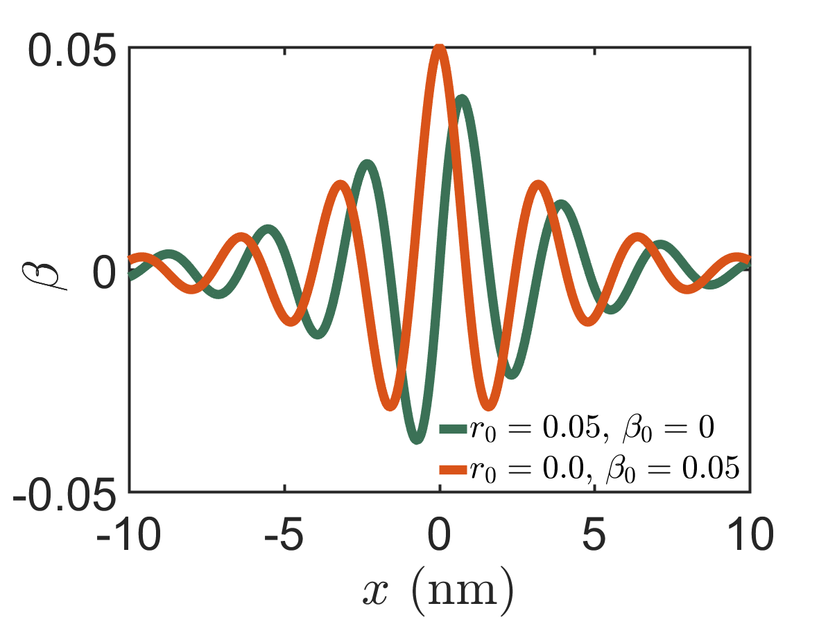
We present the variation of $r$, $k_{3}$ and $\beta$ for a protein binding at $x=0$ for two different sets of boundary conditions in fig. 2. Notice the sinusoidal correlation between the local deformation of base-pairs which is in agreement with earlier work which used Monte Carlo simulations[3, 15].
We show the deformed shapes of the helices in the fig. 3 for three cases: first when one protein binds at $x=0$, second when two proteins bind at $x=\pm 1.5$ nm, and third when two proteins bind at $x=\pm 3.5$ nm. The boundary condition for each protein is $r_{0}=0.2$ nm$,\beta_{0}=0$. We deliberately choose large values for $r_{0}$ and $\beta_{0}$ to distinguish the deformed shape from the reference shape. The large configuration changes near the site of protein binding ($x=0$) decay exponentially with distance. Note the strong overlap in the deformation fields when the distance between two proteins is $3$ nm compared to $7$ nm. This overlap results in an interaction energy between the two proteins which we subsequently quantify using eqn. (16).
We now compute the interaction energy $\Delta G$ for two proteins. The energy functional of the double helical rod is

$$E[r,\beta,k_{3}]=\frac{1}{2}EI(\kappa^{+})^{2}+\frac{1}{2}EI(\kappa^{-})^{2}+\sum_{i=1}^{3}\frac{1}{2}(L_{i}\Delta\mathbf{w}_{i}^{2}+H_{i}\hat{\eta}_{i}^{2})+K_{c}k_{3}^{2}+K_{e}\xi^{2},$$

(15)

where $\hat{\mathbf{\eta}}=\mathbf{Q}^{T}\mathbf{\eta}$ and $\Delta\mathbf{w}=\mathbf{Q}^{T}\mathbf{w}-\mathbf{Q}_{0}^{T}\mathbf{w}_{0}$. Consider two proteins, $P_{1}$ and $P_{2}$ binding at $x=0$ and $x=p$. The interaction energy $\Delta G$ defined as,

$$\begin{split}\Delta G(p)=E_{12}^{\{0,p\}}-E_{1}^{0}-E_{2}^{p},\end{split}$$

(16)

where $E_{12}^{\{0,p\}}=E[r_{12},\beta_{12},(k_{3})_{12}]$ is the energy of two proteins binding onto DNA at $x=0$ and $x=p$, while $E_{1}^{0}=E[r_{1},\beta_{1},(k_{3})_{1}]$ and $E_{2}^{p}=E[r_{2},\beta_{2},(k_{3})_{2}]$ are the energies of a single protein binding at $x=0$ and $x=p$, respectively. We linearly superimpose the strain fields from one protein ($r_{1}$ and $r_{2}$, etc) to get the resultant strain field ($r_{12}$ etc) caused by two proteins simultaneously binding to DNA.

$$\begin{split}r_{12}(x)=r_{1}(x)+r_{2}(x-p).\end{split}$$

(17)

We obtain $\beta_{12}$ and $(k_{3})_{12}$ similarly. We compute the interaction energy $\Delta G(p)$ as a function of the distance between two proteins $p$ and plot it in fig.4 together with experimental data from [5]. In excellent agreement with experiment [5] and numerical simulations [3], $\Delta G$ decays exponentially while oscillating with the period of the double helix ($\sim 10$ bp). We justify this variation of interaction energy for a simple case as follows. Consider a strain parameter $\delta(x)$ and the associated quadratic energy potential $\mathcal{E}[\delta(x)]=\int_{-\infty}^{\infty}\frac{\delta^{2}(x)}{2}\penalty\ dx$. Similar to our strain paramters in eqn. 13 let us assume $\delta(x)=Ae^{-bx}\cos(\mu x)$, then

$\displaystyle\mathcal{E}[\delta(x)]=\int_{-\infty}^{\infty}\frac{\delta^{2}(x)}{2}\penalty\ dx=\frac{A^{2}(2b^{2}+\mu^{2})}{4b(b^{2}+\mu^{2})}$

(18)

$\mathcal{E}[\delta(x-p)]=\mathcal{E}[\delta(x)]$. Now the strain obtained by superposing two strain sources a distance $p$ apart are $\delta_{2}(x)=\delta(x)+\delta(x-p)$. The energy functional corresponding to $\delta_{2}(x)$ is

	$\displaystyle\mathcal{E}[\delta_{2}(x)]=$	$\displaystyle\frac{A^{2}(2b^{2}+\mu^{2})}{2b(b^{2}+\mu^{2})}+A^{2}c_{1}e^{-bp}\sin(\mu p)+A^{2}c_{2}e^{-bp}\cos(\mu p)$
	$\displaystyle=$	$\displaystyle\mathcal{E}[\delta(x)]+\mathcal{E}[\delta(x-p)]+\Delta G$

where $c_{1}=\frac{b^{3}}{2b\mu(b^{2}+\mu^{2})}$ and $c_{2}=\frac{\mu(\mu^{2}+2b^{2}+pb^{3}+pb\mu^{2})}{2b\mu(b^{2}+\mu^{2})}$. It is notable how the decaying sinusoidal behavior of the interaction energy $\Delta G$ follows naturally from the functional form of the strain parameters and their eventual superposition.
Next, we focus on the width of the groove since many proteins are known to change the width of the major/minor groove of DNA [6, 5, 4]. We define the width of the groove, $g(x)$, as follows (we do not have a major/minor groove because $\alpha=\pi$):

$$\begin{split}g(x)=\mathbf{r}^{-}.\penalty\ \mathbf{e}_{3}(x+\frac{\pi}{2\omega})-\mathbf{r}^{+}.\penalty\ \mathbf{e}_{3}(x-\frac{\pi}{2\omega}).\end{split}$$

(19)

Note that in the reference configuration the groove width $g_{0}=\frac{\pi}{\omega}=\frac{p}{2}$. We consider a protein binding at $x=0$ and compute the change in groove width $\rho(x)=g(x)-g_{0}$ for two sets of boundary conditions, $r_{0}=0,\beta_{0}=0.02$ and $r_{0}=0.02$ nm, $\beta_{0}=0$ (see fig.4). The groove width $\rho$ decays exponentially with increasing distance from the binding site while oscillating with periodicity of the double helix. This characteristic decaying sinusoidal oscillation is documented in [3, 15] and is also observed experimentally [5]. It has been proposed that this change in groove width could explain the sinusoidally decaying interaction energy (notice the similarity of the two panels in fig.4) between two proteins bound to DNA because the binding energy of a protein binding to DNA could potentially depend on the groove width. However, we have arrived at the decaying sinusoidal variation of the interaction energy by computing the elastic energy stored in the birod without assuming any connection to the groove width.
To conclude, we have uncovered a mechanism for allostery in DNA using the theory of elastic birods. Our analysis ties together continuum theory [10], experiments [5] and numerical simulations [1, 3]. Our computations indicate that the interaction energy (eqn. (16)) for two proteins bound to DNA decays exponentially while oscillating with the period of the DNA double-helix. The decay length depends only on the elastic characteristics of the web while the oscillatory behavior is inherited from the underlying double-helical geometry. Our techniques based on a helical birod model could potentially be applied to other molecules which have a double helical geometry such as dsRNA, coiled-coil intermediate filaments, etc.

We acknowledge support from NSF through grant number NSF CMMI 1662101 and NIH through grant number NIH R01-HL 135254.

References

• [1] Tomas Drsata, Marie Zgarbova, Nada Spackova, Petr Jurecka, Jir Sponer, and Filip Lankas. Mechanical model of dna allostery. The journal of physical chemistry letters, 5(21):3831–3835, 2014.
• [2] Artem K Efremov and Jie Yan. Transfer-matrix calculations of the effects of tension and torque constraints on dna-protein interactions. arXiv preprint arXiv:1802.01437, 2018.
• [3] Chan Gu, Jun Zhang, Y Isaac Yang, Xi Chen, Hao Ge, Yujie Sun, Xiaodong Su, Lijiang Yang, Sunney Xie, and Yi Qin Gao. Dna structural correlation in short and long ranges. The Journal of Physical Chemistry B, 119(44):13980–13990, 2015.
• [4] Stephen P Hancock, Tahereh Ghane, Duilio Cascio, Remo Rohs, Rosa Di Felice, and Reid C Johnson. Control of dna minor groove width and fis protein binding by the purine 2-amino group. Nucleic acids research, 41(13):6750–6760, 2013.
• [5] Brostomer E. Xing D. Jin J. Chong S. Ge H. Wang S. Gu C. Yang L. Gao Y. Q. Su X. Sun Y. Xie X. S. Kim, S. Probing allostery through dna. Science, 339:816–819, 2013.
• [6] Mary L Kopka, Chun Yoon, David Goodsell, Philip Pjura, and Richard E Dickerson. The molecular origin of dna-drug specificity in netropsin and distamycin. Proceedings of the National Academy of Sciences, 82(5):1376–1380, 1985.
• [7] Elena F Koslover and Andrew J Spakowitz. Twist-and tension-mediated elastic coupling between dna-binding proteins. Physical review letters, 102(17):178102, 2009.
• [8] F Lankaš, Oscar Gonzalez, LM Heffler, G Stoll, M Moakher, and John H Maddocks. On the parameterization of rigid base and basepair models of dna from molecular dynamics simulations. Physical Chemistry Chemical Physics, 11(45):10565–10588, 2009.
• [9] Arpita Mitra and David Sept. Taxol allosterically alters the dynamics of the tubulin dimer and increases the flexibility of microtubules. Biophysical journal, 95(7):3252–3258, 2008.
• [10] M. Moakher and J.H. Maddocks. Double-strand elastic rod theory. Archive for rational mechanics and analysis, 177:53–91, 2005.
• [11] Kien Xuan Ngo, Nobuhisa Umeki, Saku T Kijima, Noriyuki Kodera, Hiroaki Ueno, Nozomi Furutani-Umezu, Jun Nakajima, Taro QP Noguchi, Akira Nagasaki, Kiyotaka Tokuraku, et al. Allosteric regulation by cooperative conformational changes of actin filaments drives mutually exclusive binding with cofilin and myosin. Scientific reports, 6:35449, 2016.
• [12] Naoki Ousaka and Yoshihito Inai. Transfer of noncovalent chiral information along an optically inactive helical peptide chain: allosteric control of asymmetry of the c-terminal site by external molecule that binds to the n-terminal site. The Journal of organic chemistry, 74(4):1429–1439, 2008.
• [13] Jaspreet Singh and Prashant K Purohit. Allosteric interactions in a birod model of dna. arXiv preprint arXiv:1803.04115, 2018.
• [14] Paul A Wiggins, Remus Th Dame, Maarten C Noom, and Gijs JL Wuite. Protein-mediated molecular bridging: a key mechanism in biopolymer organization. Biophysical journal, 97(7):1997–2003, 2009.
• [15] Xinliang Xu, Hao Ge, Chan Gu, Yi Qin Gao, Siyuan S Wang, Beng Joo Reginald Thio, James T Hynes, X Sunney Xie, and Jianshu Cao. Modeling spatial correlation of dna deformation: Dna allostery in protein binding. The Journal of Physical Chemistry B, 117(42):13378–13387, 2013.
1 Supplement
1.1 Expressions for quantities in main text
In this section, we give expressions for the various quantities used in the main text. In eqn. (5),
n0±=∓(cos⁡ω​x​𝐞1+sin⁡ω​x​𝐞2),b0±=∓cos⁡k⁡(−sin⁡ω​x​𝐞1+cos⁡ω​x​𝐞2)+sin⁡k​𝐞3,t0±=±sin⁡k⁡(−sin⁡ω​x​𝐞1+cos⁡ω​x​𝐞2)+cos⁡k​𝐞3,Ω0±=Ω0=ω​sin⁡k.\begin{split}&\textbf{n}^{\pm}_{0}=\mp(\cos\omega x\penalty\ \mathbf{e}_{1}+\sin\omega x\penalty\ \mathbf{e}_{2}),\\ &\textbf{b}^{\pm}_{0}=\mp\cos k(-\sin\omega x\penalty\ \mathbf{e}_{1}+\cos\omega x\penalty\ \mathbf{e}_{2})+\sin k\penalty\ \mathbf{e}_{3},\\ &\textbf{t}^{\pm}_{0}=\pm\sin k(-\sin\omega x\penalty\ \mathbf{e}_{1}+\cos\omega x\penalty\ \mathbf{e}_{2})+\cos k\penalty\ \mathbf{e}_{3},\\ &\Omega^{\pm}_{0}=\Omega_{0}=\omega\sin k.\end{split} (20)
We use the following formulas to compute n0±,b0±,t0±,Ω0±\textbf{n}^{\pm}_{0},\textbf{b}^{\pm}_{0},\textbf{t}^{\pm}_{0},\Omega^{\pm}_{0} in the reference configuration and n±,b±,t±,Ω±\textbf{n}^{\pm},\textbf{b}^{\pm},\textbf{t}^{\pm},\Omega^{\pm} in the deformed configuration:
t±=∂𝐫±∂x/|∂𝐫±∂x,Ω±=t±x.t±x,n±=1Ω±t±x.\begin{split}&\textbf{t}^{\pm}=\frac{\partial{\mathbf{r}^{\pm}}}{\partial{x}}/|\frac{\partial{\mathbf{r}^{\pm}}}{\partial{x}},\quad\Omega^{\pm}=\textbf{t}^{\pm}_{x}.\textbf{t}^{\pm}_{x},\quad\textbf{n}^{\pm}=\frac{1}{\Omega^{\pm}}\textbf{t}^{\pm}_{x}.\end{split} (21)
We use β=β++β−2\beta=\frac{\beta^{+}+\beta^{-}}{2}, βc=β+−β−2\beta^{c}=\frac{\beta^{+}-\beta^{-}}{2}, 𝐟1=cos⁡ω​x​𝐝1+sin⁡ω​x​𝐝2\penalty\ \mathbf{f}_{1}=\cos\omega x\penalty\ \mathbf{d}_{1}+\sin\omega x\penalty\ \mathbf{d}_{2} and 𝐟2=−sin⁡ω​x​𝐝1+cos⁡ω​x​𝐝2\penalty\ \mathbf{f}_{2}=-\sin\omega x\penalty\ \mathbf{d}_{1}+\cos\omega x\penalty\ \mathbf{d}_{2}. The expression for the moment transferred by the web, c, in eqn. (3) is
c=𝐐𝐇𝐐T​𝜼=H1​(−a​k3−ω​rx−a​βx)​𝐟1+H2​(−a​k3​x−ω​rx​x−a​βx​x)ω​𝐟2+H3​(βc−a​cot⁡kω​βx​xc)​𝐞3.\begin{split}\textbf{{c}}&=\mathbf{Q}\mathbf{H}\mathbf{Q}^{T}\boldsymbol{\eta}\\ &=H_{1}(-ak_{3}-\omega r_{x}-a\beta_{x})\penalty\ \mathbf{f}_{1}+H_{2}\frac{(-ak_{3x}-\omega r_{xx}-a\beta_{xx})}{\omega}\penalty\ \mathbf{f}_{2}\\ &+H_{3}(\beta^{c}-\frac{a\cot k}{\omega}\beta^{c}_{xx})\penalty\ \mathbf{e}_{3}.\end{split} (22)
The displacement between the two strands 𝐰=𝐫+−𝐫−2\mathbf{w}=\frac{\mathbf{r}^{+}-\mathbf{r}^{-}}{2} is
𝐰=(a+r)​𝐟1+a​β++β−2​𝐟2+12​∫−∞xa⁡(ξ+−ξ−)​dx​𝐞3,=(a+r)​𝐟1+a​β​𝐟2−a2​ω​βc​𝐞3.\begin{split}&\mathbf{w}=(a+r)\penalty\ \mathbf{f}_{1}+a\frac{\beta^{+}+\beta^{-}}{2}\penalty\ \mathbf{f}_{2}+\frac{1}{2}\int_{-\infty}^{x}a(\xi^{+}-\xi^{-})dx\penalty\ \mathbf{e}_{3},\\ &\penalty\ \penalty\ \penalty\ =(a+r)\penalty\ \mathbf{f}_{1}+a\beta\penalty\ \mathbf{f}_{2}-a^{2}\omega\beta^{c}\penalty\ \mathbf{e}_{3}.\end{split} (23)
We use inextensibility conditions from eqn. (4) in the main text to evaluate the integral above:
∫−∞xa⁡(ξ+−ξ−)​dx=−a2​ω​(β+−β−).\begin{split}\int_{-\infty}^{x}a(\xi^{+}-\xi^{-})dx=-a^{2}\omega(\beta^{+}-\beta^{-}).\end{split} (24)
The expression for the force exerted by the ++ strand on the −- strand, f, in eqn. (3) is
f=𝐐𝐋⁡(𝐐T​𝐰−𝐐0T​𝐰0)=L1​r​𝐟1+a​L2​cot⁡k​a​k3​x+2​ω​rx+a​βx​xω​𝐟2−L3​a2​ω2​βc+βx​xcω​𝐞3\begin{split}&\textbf{{f}}=\mathbf{Q}\mathbf{L}(\mathbf{Q}^{T}\mathbf{w}-\mathbf{Q}_{0}^{T}\mathbf{w}_{0})\\ &=L_{1}r\penalty\ \mathbf{f}_{1}+aL_{2}\cot k\frac{ak_{3x}+2\omega r_{x}+a\beta_{xx}}{\omega}\penalty\ \mathbf{f}_{2}-L_{3}a^{2}\frac{\omega^{2}\beta^{c}+\beta^{c}_{xx}}{\omega}\penalty\ \mathbf{e}_{3}\end{split} (25)
1.2 Elastic parameters for the web
To estimate the elastic parameters of the web we do as follows. We apply a stretching force FF and torque TT on one end of the double helix which changes the radius, twist and pitch. We assume these displacement variables are constant throughout the length of the deformed helix. Then we compute the elastic energy stored in the structure in terms of the strains and the unknown elastic moduli. Then we compute second derivatives of this elastic energy with respect to appropriate strains to get expressions for the stretch modulus SS, twist modulus CC, twist stretch coupling modulus gg of the double helix in terms of the elastic parameters of the birod (web and strands). Then, we get estimates for the values of the elastic constants L1,2,3,H1,2,3,Ke,KcL_{1,2,3},H_{1,2,3},K_{e},K_{c} that will reproduce the known values of S,C,gS,C,g for DNA. To begin, the position vectors are:
𝐫+=(a+r)​(cos⁡ω​x​(1+β)​𝐞1+sin⁡ω​x​(1+β)​𝐞2)+x⁡(1+e),𝐫−=−(a+r)​(cos⁡ω​x​(1+β)​𝐞1+sin⁡ω​x​(1+β)​𝐞2)+x⁡(1+e),\begin{split}&\mathbf{r}^{+}=(a+r)(\cos\omega x(1+\beta)\penalty\ \mathbf{e}_{1}+\sin\omega x(1+\beta)\penalty\ \mathbf{e}_{2})+x(1+e),\\ &\mathbf{r}^{-}=-(a+r)(\cos\omega x(1+\beta)\penalty\ \mathbf{e}_{1}+\sin\omega x(1+\beta)\penalty\ \mathbf{e}_{2})+x(1+e),\\ \end{split} (26)
We use the following basis in the forthcoming calculations.
𝐞r=cos⁡ω​x​𝐞1+sin⁡ω​x​𝐞2,𝐞θ=−sin⁡ω​x​𝐞1+cos⁡ω​x​𝐞2.\begin{split}&\penalty\ \mathbf{e}_{r}=\cos\omega x\penalty\ \mathbf{e}_{1}+\sin\omega x\penalty\ \mathbf{e}_{2},\\ &\penalty\ \mathbf{e}_{\theta}=-\sin\omega x\penalty\ \mathbf{e}_{1}+\cos\omega x\penalty\ \mathbf{e}_{2}.\end{split} (27)
As usual we assume that r,β,e∼O⁡(ε)r,\beta,e\sim O(\varepsilon) are small which allows us to linearize eqn. 26. Also rx=βx=ξx=0r_{x}=\beta_{x}=\xi_{x}=0.
𝐫+=(a+r)​𝐞r+a​ω​β​x​𝐞θ+x⁡(1+e)​𝐞3,𝐫x+=(a+r)​ω​𝐞θ+a​ω​β​𝐞θ−a​ω2​β​x​𝐞r+(1+(e​x)x)​𝐞3,=−a​ω2​β​x​𝐞r+ω⁡(a+r+a​β)​𝐞θ+(1+(e​x)x)​𝐞3.\begin{split}\mathbf{r}^{+}&=(a+r)\penalty\ \mathbf{e}_{r}+a\omega\beta x\penalty\ \mathbf{e}_{\theta}+x(1+e)\penalty\ \mathbf{e}_{3},\\ \mathbf{r}^{+}_{x}&=(a+r)\omega\penalty\ \mathbf{e}_{\theta}+a\omega\beta\penalty\ \mathbf{e}_{\theta}-a\omega^{2}\beta x\penalty\ \mathbf{e}_{r}+(1+(ex)_{x})\penalty\ \mathbf{e}_{3},\\ &=-a\omega^{2}\beta x\penalty\ \mathbf{e}_{r}+\omega(a+r+a\beta)\penalty\ \mathbf{e}_{\theta}+(1+(ex)_{x})\penalty\ \mathbf{e}_{3}.\end{split} (28)
The outer strands are inextensible, hence