Decomposition of quantitative Gaifman graphs
as a data analysis toolThanks: This research was supported by grant
TIN2017-89244-R from Ministerio de
Economia, Industria y Competitividad, and by
Conacyt (México); and
we acknowledge recognition 2017SGR-856
(MACDA) from AGAUR (Generalitat de Catalunya).
Abstract
We argue the usefulness of Gaifman graphs of first-order relational structures as an exploratory data analysis tool. We illustrate our approach with cases where the modular decompositions of these graphs reveal interesting facts about the data. Then, we introduce generalized notions of Gaifman graphs, enhanced with quantitative information, to which we can apply more general, existing decomposition notions via 2-structures; thus enlarging the analytical capabilities of the scheme. The very essence of Gaifman graphs makes this approach immediately appropriate for the multirelational data framework.
1 Introduction
First-order (finite) relational structures (see e.g. [9]) are the conceptual essence of the relational database model. Gaifman graphs are a well-known, quite natural theoretical construction that can be applied to any relational structure [9]. They have provided very interesting progress in the theory of these logical models.
Given a first-order relational structure, or relational database, with relations (or tables) , where the values in the tuples come from a fixed universe , the corresponding Gaifman graph has the elements of as vertices; and there is an edge , for , exactly when and appear together in some tuple for some table . That is, Gaifman graphs record co-occurrence (or lack thereof) among every pair of universe items.
Hence, a clique in a Gaifman graph would group items that, pairwise, appear together somewhere in the relational structure: co-occurrence patterns; a clique in its complement would reveal an incompatibility pattern. Of course, finding maximal cliques is NP-complete; but there are less demanding ways to study graphs that identify efficiently both sorts of patterns in a recursive decomposition: namely, the modular decomposition and its generalization, the decomposition of 2-structures.
This paper proposes to employ these decompositions as avenues for exploratory data analysis on relational data (whether single- or multi-relational): by applying them on the Gaifman graph of a dataset, we can obtain valuable information that would not be readily observable directly on the data.
Modular decompositions suffice to treat stardard Gaifman graphs. However, we extend the capabilities of our approach by generalizing, in very natural ways, the notion of Gaifman graph so as to handle quantitative information (a must in many data analysis applications). Hence, we develop our work using the more general decomposition of 2-structures [4]: again a notion that has been very fruitfully developed in their theoretical form, and in a number of applications (such as [8]), but not yet imported, to our knowledge, into data analysis frameworks.
2 Decomposing standard Gaifman graphs
As already mentioned, the basic notion of Gaifman graph is pretty simple: on all items that appear along all the tuples of a single- or multi-relational dataset, edges join pairs of items that appear together in some tuple.
Example 1
As a running example, let us consider a very small, single-relation database on the universe , with three attributes and three tuples:
:
:
:
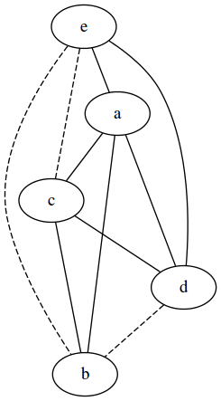
Then, the Gaifman graph is as shown in Figure 1 (left).


2.1 2-structures and their decompositions
The very classical notion called “modular decomposition” [6] suffices to implement our approach on plain Gaifman graphs; this notion has been rediscovered many times and described under several different names11 1 See https://en.wikipedia.org/wiki/Modular_decomposition for some of the alternative names that the concept has received.. However, it is insufficient to handle adequately the generalizations that we will propose below. Therefore, we develop our approach directly on top of the more general notion of 2-structures and their clans [4].
First, we describe some “cosmetics” on our Gaifman graphs: they will be seen as a complete graph with two sorts of (nonreflexive) edges. One sort corresponds to edges present in the graph (solid lines in our diagrams); the other corresponds to absent (nonreflexive) edges (broken lines). We call this graph the “natural completion” of the original graph. In our example, this process is illustrated in Figure 1 (center).
Additionally, we can label each edge with its multiplicity, that is, the number of tuples that contain the pair of items linked by the edge. The previous example then becomes as in Figure 1 (right): pairs appear either zero times together (dashed edges), once (black lines, labeled 1) or, in two cases, twice (gray lines, labeled 2).
Now, in general terms, a 2-structure is simply the complete graph on some universe , plus an equivalence relation among the edges. Figure 1 (right) serves as an example, where there are three equivalence classes of edges: the broken edges, the black edges, and the gray edges; of course, Figure 1 (center) is also an example, with just two equivalence classes of edges. We will restrict ourselves to undirected edges, and will employ the common, very graphical and intuitive representation of coloring in the same way edges belonging to the same equivalence class.
Observe that the type of the equivalence relation is because tells us whether two arbitrary edges and are equivalent.
For a 2-structure given by the set of vertices and the equivalence relation among the edges of the complete graph on , we say that a subset is a clan, informally, if all the members of are indistinguishable among them by non-members. That is: whenever some “can distinguish” between and , in the sense that the edge is not equivalent to the edge , then is not a clan. Formally (see [4]):
Definition 1
Given and an equivalence relation on the edges of the complete graph on , is a clan when
Note that different vertices outside the clan might see the clan differently: for and , and , the edges and may well be nonequivalent. We only require that each fixed does not distinguish between the clan members.
Basic examples of clans are the so-called trivial clans: all the singletons for , as well as itself, are vacuously clans. There may be other clans. For instance, consider the natural completion of the Gaifman graph obtained from Example 1, depicted in Figure 1 (center). Edges are split into two equivalence classes (existing or nonexisting edges in the original Gaifman graph). Then, one can see that there would be exactly one nontrivial clan, formed by : all vertices not in the clan (that is, vertex , the single one not in the clan) are connected to each vertex inside the clan through edges of the same color, namely solid black. Any other candidate turns out not to be a clan. For instance, any set including and but excluding is not a clan, as “distinguishes” between and ; then, any set including and must include and , which can distinguish between them. All in all, any clan including and ends up including all the vertices, that is, becoming a trivial clan. Analogous reasoning applies if we start by pairing with other vertices.
On the other hand, it is not difficult to see that the labeled, colored version of the Gaifman graph of Example 1, as depicted in Figure 1 (right), does not have nontrivial clans. Equivalence is given by the same multiplicity label (that is, edges drawn in the same “color”): the extra distinction between gray and black edges allows for external vertices to distinguish between some vertices inside every candidate proper subset. Further examples come later as clans are the key tool for our proposal of a data analysis method.
2.2 Prime clans and tree decompositions
It is known [4] that certain clans, called prime clans, allow us to decompose a 2-structure into a tree-like form.
Definition 2
For a fixed universe , we say that two subsets of overlap if neither is a subset of the other, but they are not disjoint. That is, for and , they overlap if the three sets , , and are all three nonempty. Then, prime clans are those clans that do not overlap any other clan.
Of course, trivial clans are also immediately prime clans. Thus, by definition, any two sets in the family of prime clans are either disjoint, or a subset of one another: they provide us with a so-called “decomposable set family” [11] that can be pictured in a tree form, by displaying every prime clan (except itself) as a child of the smallest prime clan that properly contains it.
There are studies that report how these decompositions look like. Specifically, at each node of the tree we have again a 2-structure, whose vertices correspond to the clans that fall as children of the node. In the case of our constructions out of Gaifman graphs, it is known that all the 2-structures that appear as nodes of such a tree decomposition are of one of two well-defined sorts: either “complete” (all edges are equivalent) or “primitive” (only having trivial clans). This is due to our graphs being undirected, because 2-structures on directed graphs may exhibit a third basic component in their tree decomposition (“linear” 2-structures). Further information on this topic appears in [4]. This reference contains, as well, often far-from-trivial proofs of theorems that ensure that things are as we have described.
Example 2
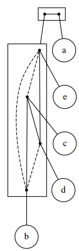
Continuing Example 1, the tree decomposition of the 2-structure in Figure 1 (center) is displayed in Figure 2 (left). Boxes correspond to clans: here, the topmost box corresponds to the trivial clan containing all the vertices and, inside it, each dot corresponds to a prime subclan. All along the whole decomposition, trivial clans are indicated by a link to the vertex they consist of, represented with an elliptic node; nontrivial ones are linked instead to a new box describing the internal structure of the clan, in terms of the prime clans it has as proper subsets. Then, as a set, each clan is formed by all the elements in the leaves of the subtree rooted at it.
A “brute-force”, exhaustive search attempt was employed in [13] to identify all prime clans. A couple of published algorithms [11, 10] can be adapted for implementing a system computing this sort of tree decompositions. However, as we envision an analysis support system able to add Gaifman nodes in an incremental manner, we have implemented a somewhat different, incremental algorithm. Due to the space limit, the details of our algorithmic contributions will be presented in a follow-up paper (or in an expanded version of this one), together with some comparisons against other algorithms.
2.3 Limits to the visualization of complex clans
Our experimentation shows that, unsurprisingly, the visualization of large Gaifman graphs is unadvisable. Actually, sometimes the clans lead to large primitive 2-structures, whose mathematical study gets pretty complicated [5]. We set up some relatively arbitrary limits, trying to get understandable diagrams. Let us consider a more realistic example to explain them.
In Figure 2 (right) we display (a fragment of) the decomposition of the Gaifman graph of the well-known Zoo dataset from the UC Irvine repository [2]; it contains 17 attributes of 100 animal species. We have preprocessed it slightly so that the semantics of each item is clearly identifiable (e. g. predator_False or toothed_True). We will return to this dataset below in Section 4.2.
For the time being, we just discuss the decomposition of its standard Gaifman graph. The topmost node of this decomposition is, as always, the trivial clan with the whole universe; in this case, it turns out to decompose as a set of many trivial clans, set up in the form of a primitive 2-structure that we choose not to draw complete; however, one nontrivial clan also appears: “mammal” and ‘milk_True” are indistinguishable from the perspective of all the other elements in the dataset. That is, for every other piece of information, either it goes together with each in some tuples (one such item could be “hair_True”), or it does not go together with any of them ever (for instance: “feathers_True”).

In our diagrams, as we do here, clans containing more than a handful of nontrivial clans are not drawn in detail: just the clan type label (“primitive” or “complete”) is shown. Besides, if there are few nontrivial clans, but many trivial ones, then the trivial clans are grouped in a single node labeled Others, sort of a merge of them all. The reader must keep in mind that this particular node actually represents together a number of unstructured items.
This approach of limiting the size of the substructures that become fully spelled-out was taken also in [8], where also a “zooming” capability was introduced (we may consider adding one such option to our system in the future).
2.4 Isolated vertex elision
As we move on, later, into quantitative generalizations of Gaifman graphs, one case turns out to be common in our experiments. Whereas Gaifman graphs do not have isolated vertices (except in limit, artificial cases such as relations with a single attribute), in our generalizations this is no longer true: many datasets will lead to 2-structures exhibiting many vertices that are endpoints only of broken edges; that is, they are isolated vertices in the corresponding (generalized) Gaifman graph. The set of those isolated vertices forms a sometimes quite large clan that clutters the diagram but contributes nothing to the analysis beyond “all these vertices are actually isolated”. We use again the label “Others” to represent these items, all alike from the decomposition perspective, as a single vertex, as indeed this is a particular case of the usage of the “Others” label as per the previous Section 2.3.
3 Interpreting a decomposition of a Gaifman graph
We move on to explain another example of our analysis strategy. We present and discuss the outcome of a tree decomposition of the Gaifman graph of a simple, famous, and relatively small dataset often used for teaching introductory data analysis courses. It comes from data of each of the passengers of the Titanic. Among several existing variants of this dataset, some of them pretty complete, we choose a reduced variant on which we illustrate the interpretation of our decompositions. This variant we use keeps four attributes, one of them (age) discretized. To describe the details of this dataset, we quote:
“The titanic dataset gives the values of four categorical attributes for each of the 2201 people on board the Titanic when it struck an iceberg and sank. The attributes are social class (first class, second class, third class, crewmember), age (adult or child), sex, and whether or not the person survived.”
(http://www.cs.toronto.edu/~delve/data/titanic/desc.html)
(As indicated in that website, this variant of the data was originally compiled by Dawson [1] and converted for use in the DELVE data analysis environment by Radford Neal.)
The decomposition via its standard Gaifman graph is depicted in Figure 3. Recall that broken edges represent pairs that never appear together in any tuple, whereas solid edges are edges of the original Gaifman graph and thus join universe elements that appear together in some tuple.
The clans for sex and survival are clear and intuitive: as they are different possible values for the same attribute, they never appear together. On the other hand, every possibility for these attributes does appear somewhere, as does every possible pairing with all other items in the universe, so that the top node is a complete 2-structure consisting on all solid edges.
Likewise, one might expect a clan with the four alternative values of traveling class, namely, 1st, 2nd, 3rd or Crew. However, that clan only has actual passenger classes. The value Crew migrates to the parent “ages” clan, where we find some interesting fact: a small primitive 2-structure arising from the interaction of the ages values and the Crew value, where of course being an adult is incompatible with being a child, and both are compatible to all the traveling classes (the top node in the middle clan); however, being in the crew is only compatible with being an adult. This calls our attention to the fact that the crew included, of course, no children, a fact that we might overlook in a non-systematic analysis. That is: even if the traveling classes and the “Crew” label are employed as values in the same column, the data tells us, through our decomposition procedure, that they have different semantics!

4 Generalizations of Gaifman graphs
We move on to discuss tree decompositions based on generalized Gaifman graphs. The aim is to keep track of quantitative information that the standard Gaifman graph lacks. In our context, many ideas present themselves to complement Gaifman graphs and clan decompositions with quantitative considerations. For the time being, we contemplate just some very simple cases: we let the number of occurrences of each pair play a role.
4.1 Thresholded Gaifman graphs
Our first variant is as follows.
Definition 3
For a threshold (a nonzero natural number) a thresholded Gaifman graph is a completion of a Gaifman graph in which each labeled edge is classified according to its number of occurrences, as follows. We still have two equivalence classes of edges. If the number in the label is above the threshold , the edge goes into one equivalence class (represented in our diagrams by a solid line); whereas if the number of occurrences of the edge is less than or equal to the threshold, then the edge belongs to the other equivalence class (and a broken line is used to represent it).
Figure 4 provides an alternative analysis of the Titanic dataset described before. There, we decompose a thresholded Gaifman graph, aiming at uncovering very common co-occurrences, that is, high multiplicities. We set the threshold rather arbitrarily at the quite high value of 1000 (out of 2201 tuples). We see at work the effect of isolated vertex elision, as many attribute values to not reach multiplicity 1000 with any other value: the elision process, as described in Section 2.4, replaces all of them by a single node, playing the same role all of them play, that is, broken lines among themselves and to all the surviving values. The new decomposition is interesting in that it very clearly reflects the Birkenhead Drill: “Women and children first”.


4.2 Quantitative Gaifman graphs
The linear colored Gaifman graph is a (completion of a) Gaifman graph in which the equivalence classes of the edges are directly defined by the label, that is, the number of occurrences. All pairs occurring once would lead to one class, those occurring twice to another, and so on; up to some limit, beyond which we do not keep the distinction. Figure 1 (right) corresponds to this case.
A natural variation is to have each color stand for some interval of values, with linearly growing limits; the case just described would correspond to intervals of width 1. Figure 5 shows one such case: we apply intervals of width 25 over the Zoo dataset. Broken lines mark less than 25 occurrences, solid lines less than 50, and the gray line appearing inside one of the clans goes beyond that limit because it gathers all birds and all fish and all insects into the oviparous clan.

This notion can be combined naturally with the previous one: instead of broken lines being simply the first interval, we can apply a different value as threshold and leave as broken lines all occurrence multiplicities below it, and then use the colors for the values at the threshold or above it, at linearly growing intervals of fixed width. Likewise, an upper threshold can be imposed. For instance, on the Titanic data, we used colors by width 1 intervals up to an upper threshold of 10: this approach is able to point out for us, with no particular user guidance, the fact that the number of children among the first-class travelers was surprisingly small: as it happened to Crew, the first-class node migrates from the traveling-class clan to the age clan.
We expect usefulness also from the exponential colored Gaifman graph: while similar in spirit to the intervals in linear graphs, here the interval width grows exponentially: each equivalence class (or color) represents an exponentially growing interval of occurrence multiplicities. On one hand, this frees the user from having to bet on a specific interval width. On the other, there are cases where the Gaifman graph multiplicities turn out to be approximately Zipfian, and the exponential coloring is likely to be adequate. Again, as with the linear case, we can also impose a user-defined threshold below which, or over which, the occurrences are not considered different; then, one runs the exponential count between them.
Even though the black-and-white printed version of this paper will not show it, we chose to provide an example of application of the exponential graph to the (“people” table within the) UW-CSE dataset from the Relational Dataset Repository (http://relational.fit.cvut.cz) at threshold 3. The items have been renamed for better understanding; also, we have manually edited out a small part of the diagram to fit the page size and to focus on the three different colors in the pairs of equivalent items: these colors tell us that the amount of Students (and thus NotProfessors) is largish (specifically 216), the quantity of year zero cases clearly smaller (namely 138) and the amount of Professors even smaller (62 in total).

5 Discussion and subsequent work
We have described a data analysis approach based on the prime tree decomposition of variations of the Gaifman graph of a dataset. We have illustrated the process with some relatively successful cases. Technologically, we have resorted to a relatively simple implementation in Python, https://github.com/MelyPic/PrimeTreeDecomposition, relying on the standard graph module NetworkX and on the graphical capabilities of the pydot interface to the Dot engine of Graphviz [7]. We have not compared the available algorithms: there is no room left for that study in this submission, and it will be the subject of forthcoming write-ups.
Many possibilities of further development remain. First and foremost, we must discuss a clear limitation. Like in so many other exploratory data analysis frameworks, for a given dataset we may not be lucky: it may happen that a given selection of Gaifman graph, once decomposed, has no nontrivial clans, or decomposes into just a few quite large primitive substructures that provide little or no insight about the data. For one, the linear Gaifman graph of the well-known toy dataset Weather (discussed e.g. in [14]) has only trivial clans and, if fully displayed, leads to just a large box of colored spaghetti. Useful advice to choose properly sorts of Gaifman graphs, thresholds, and interval widths remains to be found. After all, parameter tuning is a black art in many data mining approaches.
One natural variant consists of combining the constraints defining clans with those of standard frequent-set mining; we explored that avenue and, unfortunately, in all our attempts, we never found a single case of nontrivial clans.
Also, we can run this sort of processes on multirelational datasets or, even, directly on graphs. For the first case, our examples so far fall into the very common and standard “single table” perspective. However, from their earliest inception, Gaifman graphs were a multirelational concept by essence. Applying tree decompositions of generalized Gaifman graphs to multirelational datasets is, therefore, conceptually immediate, and indeed our example in 6 comes from a well-known multirelational benchmark. However, there, we have not taken into account the foreign key phenomenon: would it be appropriate to denormalize before computing the Gaifman graph? If so, can one compute the graph directly, efficiently, without actually denormalizing the data?
For the second case, graphs are, so to speak, their own Gaifman graph, so we can simply apply the tree decomposition on the given graph. A couple of extra possibilities naturally arise. For instance, we could decompose a 2-structure where the equivalence classes come from the lengths of the shortest paths between vertices, or from thresholding these lengths; or from the vertex- or edge-connectivity (equivalently, min-cuts, by Menger’s theorem), again possibly thresholded. Along this line, there may be interesting connections with the topic known as “blockmodeling” in social networks, which uses a notion similar to that of clan, although relaxed through allowing exceptions.
The multiplicity-based generalizations we have proposed are quite basic; more sophisticate approaches to define the equivalence relation between edges might be advantageous. In particular, we believe now that some advances might come from the study of the applicability of unsupervised discretization methods [3]. Indeed, the actual multiplicities appearing as labels of the edges of the Gaifman graph form a set of integers that is to be discretized in a number of intervals in an unsupervised manner. A few existing algorithms for unsupervised discretization can be applied to try and automatize parts of the transformation of the labeled Gaifman graph into the starting 2-structure.
Besides the theoretical developments, improving the software tool is also a desirable endeavor. Initially, we found the very notion of exploratory data analysis via 2-structure decompositions of quantitative versions of Gaifman graphs risky enough, and were not eager to compute very fast, nor in a very usable way by other people, results that, in principle, were candidates to be fully useless. However, we found our initial results clearly sufficient to consider that this approach is worth of further effort: we did design better algorithms than the ones initially employed [13], and we are confident that our tool will see considerable improvements along several facets in the coming months: the exploration of alternative tree visualizations, the implementation of additional control like zooming, or the possibility of importing the data directly from databases; this last extension is actually crucial in order to try our methods on the usual multirelational benchmarks.
References
- [1] Dawson, R.J.M.: The ’unusual episode’ data revisited. Journal of Statistics Education 3(3) (1995)
- [2] Dheeru, D., Karra Taniskidou, E.: UCI machine learning repository (2017), http://archive.ics.uci.edu/ml
- [3] Dougherty, J., Kohavi, R., Sahami, M.: Supervised and unsupervised discretization of continuous features. In: Prieditis, A., Russell, S.J. (eds.) Machine Learning, Proceedings of the Twelfth International Conference on Machine Learning, Tahoe City, California, USA, July 9-12, 1995. pp. 194–202. Morgan Kaufmann (1995)
- [4] Ehrenfeucht, A., Harju, T., Rozenberg, G.: The Theory of 2-Structures - A Framework for Decomposition and Transformation of Graphs. World Scientific (1999), http://www.worldscibooks.com/mathematics/4197.html
- [5] Ehrenfeucht, A., Rozenberg, G.: Primitivity is hereditary for 2-structures. Theor. Comput. Sci. 70(3), 343–358 (1990), https://doi.org/10.1016/0304-3975(90)90131-Z
- [6] Gallai, T.: Transitiv orientierbare graphen. Acta Mathematica Academiae Scientiarum Hungarica 18(1), 25–66 (1967), http://dx.doi.org/10.1007/BF02020961
- [7] Gansner, E.R., North, S.C.: An open graph visualization system and its applications to software engineering. SOFTWARE - PRACTICE AND EXPERIENCE 30(11), 1203–1233 (2000)
- [8] Larraz, D.: Aplicación de las 2-estructuras a las gramáticas del lenguaje humano y representación gráfica de ambas. Graduation Project, Universidad de Zaragoza (2010), http://zaguan.unizar.es/record/5000
- [9] Libkin, L.: Elements of Finite Model Theory. Texts in Theoretical Computer Science. An EATCS Series, Springer (2004), https://doi.org/10.1007/978-3-662-07003-1
- [10] McConnell, R.M.: An O(n2) incremental algorithm for modular decomposition of graphs and 2-structures. Algorithmica 14(3), 229–248 (1995), https://doi.org/10.1007/BF01206330
- [11] McConnell, R.M., Spinrad, J.P.: Modular decomposition and transitive orientation. Discrete Mathematics 201(1), 189 – 241 (1999), http://www.sciencedirect.com/science/article/pii/S0012365X98003197
- [12] Padhy, N., Panigrahi, R.: Multi relational data mining approaches: A data mining technique. CoRR abs/1211.3871 (2012), http://arxiv.org/abs/1211.3871
- [13] Rodríguez-Navas, L.: Estructures de grafs amb equivalències d’arestes aplicades a l’anàlisi de dades relacionals. Graduation Project, FIB, UPC (2017)
- [14] Witten, I.H., Eibe, F., Hall, M.A.: Data mining: practical machine learning tools and techniques, 3rd Edition. Morgan Kaufmann, Elsevier (2011), http://www.worldcat.org/oclc/262433473