An interface-unfitted finite element method for elliptic interface optimal control problem Thanks: This work is partially supported by National Natural Science Foundation of China under grant 11771312, 11471231 and 11401404.

Chao Chao Yang ^†^†thanks: Email: yangchaochao9055@163.com Tao Wang ^†^†thanks: Email: 602721197@qq.com Xiaoping Xie ^†^†thanks: Corresponding author. Email: xpxie@scu.edu.cn Affiliation: School of Mathematics, Sichuan University, Chengdu 610064, China

Abstract

This paper develops and analyses numerical approximation for linear-quadratic optimal control problem governed by elliptic interface equations. We adopt variational discretization concept to discretize optimal control problem, and apply an interface-unfitted finite element method due to [A. Hansbo and P. Hansbo. An unfitted finite element method, based on Nitsche’s method, for elliptic interface problems. Comput. Methods Appl. Mech. Engrg., 191(47-48): 5537-5552, 2002] to discretize corresponding state and adjoint equations, where piecewise cut basis functions around interface are enriched into standard conforming finite element space. Optimal error estimates in both $L^{2}$ norm and a mesh-dependent norm are derived for optimal state, co-state and control under different regularity assumptions. Numerical results verify the theoretical results.

Keywords interface equations, interface control, variational discretization concept, cut finite element method

MSC(2010) 65K15, 65N30

1 Introduction

Many optimization processes in science and engineering lead to optimal control problems governed by partial differential equations (pdes). In particular in some practical problems, such as the multi-physics progress or engineering design with different materials, the corresponding controlled systems are described by elliptic equations with interface, whose coefficients are discontinuous across the interface.

Let’s consider the following linear-quadratic optimal control problem governed by elliptic interface equations:

\text{min}~J(y,u):=\frac{1}{2}\int_{\Omega}(y-y_{d})^{2}~dx+\frac{\alpha}{2}\int_{\Gamma}u^{2}~ds

(1.1)

for $(y,u)\in H^{1}_{0}(\Omega)\times L^{2}(\Gamma)$ subject to the elliptic interface problem

\left\{\begin{array}[]{rll}&-\nabla\cdot(a(x)\nabla y)=f,&\text{ in }\Omega\\ &y=0,&\text{ on }\partial\Omega\\ &[y]=0,[a\nabla_{n}y]=g+u,&\text{ on }\Gamma\\ \end{array}\right.

(1.2)

with the control constraint

u_{a}\leq u\leq u_{b},\text{ a.e. on }\Gamma.

(1.3)

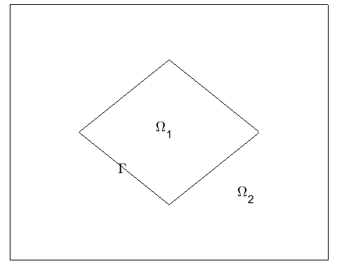
Here $\Omega\subseteq\mathbb{R}^{d}(d=2,3)$ is a polygonal or polyhedral domain, consisting of two disjoint subdomains $\Omega_{i}(1\leq i\leq 2)$ , and interface $\Gamma=\partial\Omega_{1}\cap\partial\Omega_{2}$ ; see Figure 1 for an illustration. $y_{d}\in L^{2}(\Omega)$ is the desired state to be achieved by controlling $u$ through interface $\Gamma$ , and $\alpha$ is a positive constant. $a(\cdot)$ is piecewise constant with

a|_{\Omega_{i}}=a_{i}>0,i=1,2.

$[y]:=(y|_{\Omega_{1}})|_{\Gamma}-(y|_{\Omega_{2}})|_{\Gamma}$ is the jump of function $y$ across interface $\Gamma$ , $\nabla_{n}y=n\cdot\nabla y$ is the normal derivative of $y$ with $n$ denoting the unit outward normal vector along $\partial\Omega_{1}\cap\Gamma$ ,

f\in L^{2}(\Omega),\quad g\in H^{1/2}(\Gamma),\quad\text{ and }u_{a},u_{b}\in H^{1/2}(\Gamma)\ \text{ with $u_{a}\leq u_{b}$ a.e. on $\Gamma$}.

(1.4)

The choice of homogeneous boundary condition on boundary $\partial\Omega$ is made for ease of presentation, since similar results are valid for other boundary conditions.

Refer to caption — Figure 1: The geometry of an interface problem: an illustration

For elliptic interface problem, the global regularity of its solution is often low due to the discontinuity of coefficient $a(\cdot)$ . The low global regularity may result in reduced accuracy for its finite element approximations [1, 55], especially when the interface has complicated geometrical structure [29, 40]. Generally there have two categories in literature to tackle this difficulty, i.e. interface(or body)-fitted methods [2, 7, 15, 28, 46, 33, 56, 11, 59, 16] and interface-unfitted methods. For the interface-fitted methods, meshes aligned with the interface are used so as to dominate the approximation error caused by the non-smoothness of solution. In practice, it is usually difficult to construct such meshes, especially in three-dimensional problems.

In contrast, the interface-unfitted methods, with certain types of modifications for approximating functions around interface, do not require the meshes to fit the interface, and thus avoid complicated mesh generation. For some representative interface-unfitted methods, we refer to the extended/generalized finite element method [42, 43, 44, 51, 5], where additional basis functions characterizing the singularity of solution around interface are enriched into the approximation space, and the immersed finite element method (IFEM) [36, 12, 35, 17, 37, 23, 38], which uses special finite element basis functions satisfying the interface jump conditions in a certain sense.

In [20] an interface-unfitted finite element method based on Nitsche’s approach [45] was proposed for elliptic interface equations. In this method, piecewise linear cut basis functions around interface are added into the standard linear finite element space, and corresponding parameter in the Nitsche’s numerical fluxes on each element intersected by interface are chosen to depend on the relative area/volume of the two parts aside interface. This method was later named as CutFEM in [21, 10, 13, 49]. In fact, this method can be viewed as an extended finite element method combined with Nitsche’s approach, which is also called as Nitsche-XFEM [3, 32]. As shown in [20], the CutFEM yields optimal order convergence, i.e. second order convergence in $L^{2}$ -norm on a non-degenerate triangulation.

For optimal control problem governed by elliptic pdes with smooth coefficients $a(\cdot)$ and with the control $u$ acting in whole domain $\Omega$ or on boundary $\partial\Omega$ , a lot of finite element methods have been studied; see, e.g. [4, 34, 25, 6, 41, 24, 14, 47, 31, 48, 18, 54, 57, 47]. However, there are limited literature on the numerical analysis for optimal control problems governed by elliptic interface equations. [58] developed a numerical method, based on the variational discretization concept (cf.[25, 26]), for the case of distributed control, i.e. control $u$ acting in $\Omega$ through

-\nabla\cdot(a(x)\nabla y)=f+u,

where the IFEM is applied to discretize the state equation with homogeneous interface jump condition

[a\nabla_{n}y]=0,\quad\text{ on }\Gamma.

Optimal error estimates were derived for the control, state and co-state on uniform triangulations. We note that it is usually difficult to extend the IFEM to the case of non-homogeneous interface conditions [22, 19, 30]. [53] investigated $hp$ -finite elements for the model problem (1.1)-(1.3) on interface-fitted meshes, and didn’t give optimal convergence rates for the state and control in $L^{2}$ norm.

In this paper, we’ll also adopt the variational discretization concept to discretize the optimal control problem (1.1)-(1.3), and apply the CutFEM on interface-unfitted meshes for the state and co-state equations. Optimal error estimates in both $L^{2}$ norm and a mesh-dependent norm will be derived for the optimal state, co-state, and control under different regularity assumptions.

The rest of this paper is organized as follows. In Section 2, we give some notations and optimality conditions for the optimal control problem. Section 3 sketches the CutFEM briefly, then complements error estimates of the CutFEM in fractional Sobolev space $H^{3/2}$ . In Section 4, we firstly give the discrete optimal control problem and its optimality conditions, then derives error estimates for the state ,co-state and control of the optimal control problem. Finally, Section 5 provides numerical examples to verify our theoretical results.

2 Notation and optimality conditions

For bounded domain $\Lambda\subset\mathbb{R}^{d}$ and non-negative integer $m$ , let $H^{m}(\Lambda)$ and $H^{m}_{0}(\Lambda)$ denote the standard Sobolev spaces on $\Lambda$ with norm $\|\cdot\|_{m,\Lambda}$ and semi-norm $|\cdot|_{m,\Lambda}$ . In particular, $L^{2}(\Lambda):=H^{0}(\Lambda)$ , with the standard $L^{2}$ -inner product $(\cdot,\cdot)_{\Lambda}$ . We also need the fractional Sobolev space

H^{m+\frac{1}{2}}(\Lambda):=\{w\in H^{m}(\Lambda):\sum_{|\alpha|=m}\iint_{\Lambda\times\Lambda}\frac{|D^{\alpha}w(s)-D^{\alpha}w(t)|^{2}}{|s-t|^{d+1}}~dsdt<\infty\}

with norm

\|w\|_{m+\frac{1}{2},\Lambda}:=\left(\|w\|_{m,\Lambda}^{2}+\sum_{|\alpha|=m}\iint_{\Lambda\times\Lambda}\frac{|D^{\alpha}w(s)-D^{\alpha}w(t)|^{2}}{|s-t|^{d+1}}~dsdt\right)^{\frac{1}{2}}.

For $s\in\mathbb{R}^{+}$ , let’s define

H^{s}(\Omega_{1}\cup\Omega_{2}):=\left\{w\in L^{2}(\Omega):\ w|_{\Omega_{i}}\in H^{s}(\Omega_{i}),\ i=1,2\right\}

with norm $\|\cdot\|_{s,\Omega_{1}\cup\Omega_{2}}:=\left(\sum_{i=1}^{2}\|\cdot\|_{s,\Omega_{i}}^{2}\right)^{\frac{1}{2}}$ .

The weak formulation of state equation (1.2) reads: find $y\in H_{0}^{1}(\Omega)$ satisfying

a(y,w)=(f,w)_{\Omega}+(g+u,w)_{\Gamma},~~\forall w\in H_{0}^{1}(\Omega).

(2.1)

Where $a(y,w):=(a\nabla y,\nabla w)_{\Omega}.$

In order to get convergence order of finite element methods, let’s make the following regularity assumptions for above interface equations.

(R1).

If $g+u\in L^{2}(\Gamma)$ , then the weak solution $y$ of (2.1) satisfies $y\in H_{0}^{1}(\Omega)\cap H^{3/2}(\Omega_{1}\cup\Omega_{2})$ and

$\|y\|_{\frac{3}{2},\Omega_{1}\cup\Omega_{2}}\lesssim\|f\|_{L^{2}(\Omega)}+\|g+u\|_{L^{2}(\Gamma)}.$
(R2).

If $g+u\in H^{1/2}(\Gamma)$ , then the weak solution $y$ of (2.1) satisfies $y\in H_{0}^{1}(\Omega)\cap H^{2}(\Omega_{1}\cup\Omega_{2})$ and

$\|y\|_{2,\Omega_{1}\cup\Omega_{2}}\lesssim\|f\|_{L^{2}(\Omega)}+\|g+u\|_{\frac{1}{2},\Gamma}.$

Here and in what follows, we use “ $\bar{a}\lesssim\bar{b}$ ” to denote that, there is a generic positive constant $C$ , independent of the mesh parameter $h$ and the location of interface relative to the mesh, such that “ $\bar{a}\leq C\bar{b}$ . “ $\bar{a}\approx\bar{b}$ ” means “ $\bar{a}\lesssim\bar{b}\lesssim\bar{a}$ ”.

Remark 2.1.

Let’s point out that the above assumptions are reasonable. In fact, for the assumption (R1), if $\Omega$ and $\Gamma$ are smooth with $\Gamma\cap\partial\Omega=\emptyset$ , then (R1) holds [7, (2.2)]. And it has been shown in [53, Corollary 4.12] that (R1) holds if $\Omega\subset\mathbb{R}^{2}$ and its subdomains $\Omega_{i}$ are all polygonal. For the assumption (R2), if the domain $\Omega$ is convex, and the interface $\Gamma$ is $C^{2}$ continuous with $\Gamma\cap\partial\Omega=\emptyset$ , then (R2) also holds [15, theorem 2.1].

For the boxed control constraint

U_{ad}:=\{u\in L^{2}(\Gamma):u_{a}\leq u\leq u_{b},\text{ a.e. on }\Gamma\},

by standard optimality techniques, we can easily derive existence and uniqueness results and optimality conditions for the optimal control problem.

Lemma 2.1.

The optimal control problem (1.1)-(1.3) admits a unique solution $(y^{*},u^{*})\in H^{1}_{0}(\Omega)\times U_{ad}$ , and the equivalent optimality conditions read: find $(y^{*},p^{*},u^{*})\in H_{0}^{1}(\Omega)\times H_{0}^{1}(\Omega)\times U_{ad}$ such that

		$\displaystyle a(y^{},w)=(f,w)_{\Omega}+(g+u^{},w)_{\Gamma},~~\forall w\in H_{0}^{1}(\Omega),$		(2.2)
		$\displaystyle a(w,p^{})=(y^{}-y_{d},w)_{\Omega},~~\forall w\in H_{0}^{1}(\Omega),$		(2.3)
		$\displaystyle(p^{}+\alpha u^{},u-u^{*})_{\Gamma}\geq 0,~~\forall u\in U_{ad}.$		(2.4)

Proof.

For the sake of completeness, we give a brief proof. For $u\in L^{2}(\Gamma)$ , the weak problem (2.1) admits a unique weak solution $y=y(u)$ . Let’s introduce a reduced functional $\tilde{J}(u):=J(y(u),u)$ . Then the existence and uniqueness of $u$ follow from that $\tilde{J}(\cdot)$ is strictly convex and continuous in $U_{ad}$ . The equations (2.2)-(2.4) are necessary conditions for the optimal control problem (1.1)-(1.3). And, from the convexity of $J(\cdot)$ , they are also sufficient conditions (cf. [39, 52]). ∎

Remark 2.2.

We note that (2.3) is the so-called adjoint equations, and $p^{*}$ is the co-state, which is the weak solution of following interface equations

\left\{\begin{array}[]{rll}&-\nabla\cdot(a(x)\nabla p^{*})=y^{*}-y_{d},&\text{ in }\Omega,\\ &p^{*}=0,&\text{ on }\partial\Omega,\\ &[p^{*}]=0,[a\nabla_{n}p^{*}]=0.&\text{ on }\Gamma.\end{array}\right.

Remark 2.3.

The variational inequality (2.4) means that

u^{*}=P_{U_{ad}}(-\frac{1}{\alpha}p^{*}|_{\Gamma}),

(2.5)

where $P_{U_{ad}}$ denotes the $L^{2}-$ projection onto $U_{ad}$ [9].

Lemma 2.2.

Assume that (1.4) holds, and let $(y^{*},u^{*})\in H^{1}_{0}(\Omega)\times U_{ad}$ be the solution to the optimal control problem (1.1)-(1.3). Then, under the assumption (R2), we have $u^{*}\in H^{1/2}(\Gamma),y^{*}\in H^{2}(\Omega_{1}\cup\Omega_{2})$ , and

\|y^{*}\|_{2,\Omega_{1}\cup\Omega_{2}}\lesssim\|f\|_{L^{2}(\Omega)}+\|g\|_{\frac{1}{2},\Gamma}+\|u^{*}\|_{\frac{1}{2},\Gamma}.

(2.6)

Proof.

From (R2), it suffices to show $u^{*}\in H^{1/2}(\Gamma)$ . Since $p^{*}\in H^{1}(\Omega)$ , from (2.5) it follows $u^{*}=P_{U_{ad}}(-\frac{1}{\alpha}p^{*}|_{\Gamma})\in U_{ad}$ . As the control constraint in $U_{ad}$ is a boxed one with $u_{a},u_{b}\in H^{1/2}(\Gamma)$ , we obtain $u^{*}\in H^{1/2}(\Gamma)$ (cf. [52]). ∎

3 CutFEM for state and co-state equations

We know that the optimal state $y^{*}$ and co-state $p^{*}$ of (2.2)-(2.4) can respectively be viewed as solutions to the following two interface problems.

Find $y^{*}\in H_{0}^{1}(\Omega)$ such that

a(y^{*},w)=(f,w)_{\Omega}+(g+u^{*},w)_{\Gamma},~~\forall w\in H_{0}^{1}(\Omega).

(3.1)

Find $p^{*}\in H_{0}^{1}(\Omega)$ such that

a(w,p^{*})=(y^{*}-y_{d},w)_{\Omega},~~\forall w\in H_{0}^{1}(\Omega).

(3.2)

3.1 Cut finite element schemes

Let $\mathscr{T}_{h}$ be a shape-regular triangulation of $\Omega$ consisting of open triangles/tetrahedrons, and mesh size $h=\max_{K\in\mathscr{T}_{h}}h_{K}$ , where $h_{K}$ denotes the diameter of $K\in\mathscr{T}_{h}$ . We mention that $\mathscr{T}_{h}$ is independent of the location of interface, and elements of $\mathscr{T}_{h}$ fall into the following three classes:

		$\displaystyle G_{h}:=\{K\in\mathscr{T}_{h}:K\cap\Gamma\neq\emptyset\},$
		$\displaystyle\bar{G}_{i,h}:=\{K\in\mathscr{T}_{h}:K\notin G_{h}\text{ and }K\subset\Omega_{i}\},\quad i=1,2.$

For element $K\in G_{h}$ , which is called as interface element, let’s set $K_{i}:=K\cap\Omega_{i}(i=1,2),\Gamma_{K}:=\Gamma\cap K$ , and denote by $\Gamma_{K,h}$ the straight line/plane connecting the intersection between $\Gamma$ and $\partial K$ .

For ease of discussion, we make the following assumptions on $\mathscr{T}_{h}$ and $\Gamma$ (cf. [20, 49]).

(A1).

For $K\in G_{h}$ and an edge/face $F\subset\partial K$ , $\Gamma\cap F$ is simply connected.
(A2).

For $K\in G_{h}$ , there is a piecewise smooth function $\delta$ which maps $\Gamma_{K,h}$ to $\Gamma_{K}$ .

Remark 3.1.

Assumptions (A1)-(A2) are easy to satisfy. In $\mathbb{R}^{2}$ , (A1) means that the interface $\Gamma$ intersects each edge of interface element $K\in G_{h}$ at most once. And (A2) means that the part of interface $\Gamma$ contained in each interface element $K\in G_{h}$ is piecewise smooth.

Now let’s introduce finite dimensional spaces, for $i=1,2$ ,

\displaystyle V_{i}^{h}:=\{\phi\in H^{1}(\Omega_{i}):\phi|_{K_{i}}\text{ is a linear polynomial},~\forall K\in G_{h}\cup\bar{G}_{i,h},\text{ and }\phi|_{\partial\Omega\cap\partial\Omega_{i}}=0\},

\displaystyle V^{h}:=\left\{\phi\in L^{2}(\Omega):\phi|_{\Omega_{i}}\in V_{i}^{h},\ i=1,2\right\},

(3.3)

and define two functions $\kappa_{1},\kappa_{2}$ on $\Gamma$ by

\kappa_{i}|_{\Gamma_{K}}=\frac{|K_{i}|}{|K|},\forall K\in G_{h}~~(i=1,2),

where $|K_{i}|$ and $|K|$ denote the area/volume of $K_{i}$ and $K$ respectively. It is evident that

\kappa_{1}+\kappa_{2}=1.

For $\phi\in V^{h}$ , we set $\phi_{i}:=\phi|_{\Omega_{i}}$ for $i=1,2$ , and

\{\phi\}:=\kappa_{1}\cdot\phi_{1}|_{\Gamma}+\kappa_{2}\cdot\phi_{2}|_{\Gamma}.

Then the cut finite element schemes for (3.1) and (3.2) are described respectively as follows:

Find $y^{h}\in V^{h}$ such that

a_{h}(y^{h},w_{h})=(f,w_{h})_{\Omega}+(g+u^{*},\kappa_{2}w_{h,1}+\kappa_{1}w_{h,2})_{\Gamma},\quad\forall w_{h}\in V^{h}.

(3.4)

Find $p^{h}\in V^{h}$ such that

a_{h}(p^{h},w_{h})=(y^{*}-y_{d},w_{h})_{\Omega},\quad\forall w_{h}\in V^{h}.

(3.5)

The modified bilinear form $a_{h}(\cdot,\cdot)$ is given by

	$\displaystyle a_{h}(y^{h},w_{h}):=$	$\displaystyle\sum_{i=1}^{2}(a\nabla y^{h},\nabla w_{h})_{\Omega_{i}}$
		$\displaystyle-([y^{h}],\{a\nabla_{n}w_{h}\})_{\Gamma}-(\{a\nabla_{n}y^{h}\},[w_{h}])_{\Gamma}+\lambda([y^{h}],[w_{h}])_{\Gamma},$

and the stabilization parameter $\lambda$ is taken as

\lambda|_{K}=\widetilde{C}h_{K}^{-1}\max\{a_{1},a_{2}\},

(3.6)

with the constant $\widetilde{C}>0$ sufficiently large.

Let’s introduce a mesh-dependent semi-norm $|||\cdot|||$ in $H^{3/2}(\Omega_{1}\cup\Omega_{2})$ with

|||w|||^{2}:=|w|_{1,\Omega_{1}\cup\Omega_{2}}^{2}+\|[w]\|_{\frac{1}{2},h,\Gamma}^{2}+\|\{\nabla_{n}w\}\|_{-\frac{1}{2},h,\Gamma}^{2},\quad\forall w\in H^{3/2}(\Omega_{1}\cup\Omega_{2}),

where

\|\cdot\|_{\frac{1}{2},h,\Gamma}^{2}:=\sum_{K\in G_{h}}h_{k}^{-1}\|\cdot\|_{0,\Gamma_{K}}^{2},~~\|\cdot\|_{-\frac{1}{2},h,\Gamma}^{2}:=\sum_{K\in G_{h}}h_{K}\|\cdot\|_{0,\Gamma_{K}}^{2}.

It is easy to see that $|||\cdot|||$ is a norm on $V^{h}$ and it holds

||w_{h}||_{0,\Omega}\lesssim|w_{h}|_{1,\Omega_{1}\cup\Omega_{2}}\leq|||w_{h}|||,\quad\forall w_{h}\in V^{h}.

(3.7)

Then we have the following boundedness and coerciveness for the bilinear form $a_{h}(\cdot,\cdot)$ (cf. [20, Lemma 5]):

Lemma 3.1.

It holds

a_{h}(y,w)\lesssim|||y|||\ |||w|||,\quad\forall y,w\in H^{3/2}(\Omega_{1}\cup\Omega_{2}).

(3.8)

In addition, if $\widetilde{C}$ of (3.6) is chosen to be sufficiently large, then

a_{h}(w_{h},w_{h})\gtrsim|||w_{h}|||^{2},\quad\forall w_{h}\in V^{h}.

(3.9)

Remark 3.2.

As shown in [20, lemma 1], the schemes (3.4)-(3.5) are consistent with respect to the weak solutions $y^{*},p^{*}\in H^{1}_{0}(\Omega)$ of problems (3.1)-(3.2) respectively in the following sense: for $w_{h}\in V^{h}$ , we have

a_{h}(y^{*}-y^{h},w_{h})=0,\quad a_{h}(p^{*}-p^{h},w_{h})=0.

(3.10)

From [20], the following results of existence, uniqueness, and error estimates hold:

Lemma 3.2.

Assume $g,u^{*}\in H^{1/2}(\Gamma)$ , and $y^{*},p^{*}\in H^{1}_{0}(\Omega)\cap H^{2}(\Omega_{1}\cup\Omega_{2})$ be the solutions to continuous problems (3.1)-(3.2) respectively. If $\widetilde{C}$ of (3.6) is chosen to be sufficiently large, then (i) The discrete scheme (3.4) admits a unique solution $y^{h}\in V^{h}$ such that

	$\displaystyle\|\|\|y^{}-y^{h}\|\|\|\lesssim h\\|y^{}\\|_{2,\Omega_{1}\cup\Omega_{2}},$		(3.11)
	$\displaystyle\\|y^{}-y^{h}\\|_{0,\Omega}\lesssim h^{2}\\|y^{}\\|_{2,\Omega_{1}\cup\Omega_{2}}.$		(3.12)

(ii) The discrete scheme (3.5) admits a unique solution $p^{h}\in V^{h}$ such that

	$\displaystyle\|\|\|p^{}-p^{h}\|\|\|\lesssim h\\|p^{}\\|_{2,\Omega_{1}\cup\Omega_{2}},$		(3.13)
	$\displaystyle\\|p^{}-p^{h}\\|_{0,\Omega}\lesssim h^{2}\\|p^{}\\|_{2,\Omega_{1}\cup\Omega_{2}}.$		(3.14)

Remark 3.3.

We note that the error estimates in above lemma require that $y^{*},p^{*}\in H^{2}(\Omega_{1}\cup\Omega_{2})$ . For $y^{*}$ , this means that $g+u^{*}\in H^{1/2}(\Gamma)$ (cf. [20] and the assumption (R2)). In next section, we’ll derive estimates under mild regularity assumptions, say $y^{*},p^{*}\in H^{3/2}(\Omega_{1}\cup\Omega_{2})$ .

3.2 Alternative error estimates of CutFEM

For $i=1,2$ , let $E_{i}:\left\{w\in H^{\frac{3}{2}}(\Omega_{i}):\ w|_{\partial\Omega_{i}\setminus\Gamma}=0\right\}\longrightarrow H^{\frac{3}{2}}(\Omega)\cap H^{1}_{0}(\Omega)$ be the extension operators satisfying that, for $w\in H^{\frac{3}{2}}(\Omega_{1}\cup\Omega_{2})\cap H^{1}_{0}(\Omega)$ with $w_{i}:=w|_{\Omega_{i}}$ , we have

E_{i}w_{i}|_{\Omega_{i}}=w_{i},\quad\|E_{i}w_{i}\|_{s,\Omega}\lesssim\|w_{i}\|_{s,\Omega_{i}},~0\leq s\leq\frac{3}{2}.

(3.15)

Let $I_{h}:H^{1}_{0}(\Omega)\longrightarrow\{w\in C(\bar{\Omega}):w|_{K}\text{ is linear },\forall K\in\mathscr{T}_{h},\text{ and }w|_{\partial\Omega}=0\}$ denote the Scott-Zhang interpoation operator [50]. Then for $K\in\mathscr{T}_{h}$ and $m=1,2$ , we have

\|w-I_{h}w\|_{j,K}\lesssim h_{K}^{m-j}\|w\|_{m,S_{K}},\quad\forall w\in H^{m}(\Omega)\cap H^{1}_{0}(\Omega),\ j=0,1

where $S_{K}:=\text{interior}\{\cup\bar{T}:T\in\mathscr{T}_{h},\bar{T}\cap\bar{K}\neq\emptyset\}$ . Thus, by using the real interpolation method (cf. the proof of [8, Theorem (14.3.3)]), it’s easy to get estimation

\|w-I_{h}w\|_{j,K}\lesssim h_{K}^{\frac{3}{2}-j}\|w\|_{\frac{3}{2},S_{K}},\forall w\in H^{\frac{3}{2}}(\Omega)\cap H^{1}_{0}(\Omega),\ K\in\mathscr{T}_{h},\ j=0,1.

(3.16)

Now we construct an interpolation operator $I_{h}^{*}:H^{1}_{0}(\Omega)\cap H^{\frac{3}{2}}(\Omega_{1}\cup\Omega_{2})\longrightarrow V^{h}$ with

(I_{h}^{*}w)|_{\Omega_{i}}:=(I_{h}E_{i}w_{i})|_{\Omega_{i}},\quad i=1,2.

(3.17)

Lemma 3.3.

For $w\in H^{1}_{0}(\Omega)\cap H^{\frac{3}{2}}(\Omega_{1}\cup\Omega_{2})$ , we have

|||w-I_{h}^{*}w|||\lesssim h^{\frac{1}{2}}\|w\|_{\frac{3}{2},\Omega_{1}\cup\Omega_{2}}.

(3.18)

Proof.

For $w\in H^{1}_{0}(\Omega)\cap H^{\frac{3}{2}}(\Omega_{1}\cup\Omega_{2})$ with $w_{i}:=w|_{\Omega_{i}}$ $(i=1,2)$ , from (3.15)-(3.17) it follows

	$\displaystyle\|w-I_{h}^{*}w\|_{1,\Omega_{1}\cup\Omega_{2}}^{2}$	$\displaystyle=\sum_{i=1}^{2}\sum_{K\in\mathscr{T}_{h}}\|w_{i}-I_{h}E_{i}w_{i}\|_{1,K\cap\Omega_{i}}^{2}=\sum_{i=1}^{2}\sum_{K\in\mathscr{T}_{h}}\|E_{i}w_{i}-I_{h}E_{i}w_{i}\|_{1,K\cap\Omega_{i}}^{2}$
		$\displaystyle\lesssim\sum_{i=1}^{2}h\\|E_{i}w_{i}\\|_{\frac{3}{2},\Omega}^{2}\lesssim\sum_{i=1}^{2}h\\|w_{i}\\|_{\frac{3}{2},\Omega_{i}}^{2}\lesssim h\\|w\\|_{\frac{3}{2},\Omega_{1}\cup\Omega_{2}}^{2}.$

In light of (3.15)-(3.17) and the trace inequality, we have

	$\displaystyle\\|[w-I_{h}^{*}w]\\|_{\frac{1}{2},h,\Gamma}^{2}$	$\displaystyle\lesssim\sum_{i=1}^{2}\sum_{K\in G_{h}}h_{K}^{-1}\\|w_{i}-I_{h}E_{i}w_{i}\\|_{0,\Gamma_{K}}^{2}=\sum_{i=1}^{2}\sum_{K\in G_{h}}h_{K}^{-1}\\|E_{i}w_{i}-I_{h}E_{i}w_{i}\\|_{0,\Gamma_{K}}^{2}$
		$\displaystyle\lesssim\sum_{i=1}^{2}\sum_{K\in G_{h}}(h_{K}^{-2}\\|E_{i}w_{i}-I_{h}E_{i}w_{i}\\|_{0,K}^{2}+\\|E_{i}w_{i}-I_{h}E_{i}w_{i}\\|_{1,K}^{2})$
		$\displaystyle\lesssim\sum_{i=1}^{2}\sum_{K\in G_{h}}h_{K}\\|E_{i}w_{i}\\|_{\frac{3}{2},S_{K}}^{2}$
		$\displaystyle\lesssim\sum_{i=1}^{2}h\\|E_{i}w_{i}\\|_{\frac{3}{2},\Omega}^{2}\lesssim\sum_{i=1}^{2}h\\|w_{i}\\|_{\frac{3}{2},\Omega_{i}}^{2}\lesssim h\\|w\\|_{\frac{3}{2},\Omega_{1}\cup\Omega_{2}}^{2}.$

Similarly, we obtain

	$\displaystyle\\|\{\nabla_{n}(w-I_{h}^{*}w)\}\\|_{-\frac{1}{2},h,\Gamma}^{2}$	$\displaystyle\lesssim\sum_{i=1}^{2}\sum_{K\in G_{h}}h_{K}\\|\nabla_{n}(w_{i}-I_{h}E_{i}w_{i})\\|_{0,\Gamma_{K}}^{2}$
		$\displaystyle\lesssim\sum_{i=1}^{2}\sum_{K\in G_{h}}h_{K}\\|E_{i}w_{i}\\|_{\frac{3}{2},K}^{2}$
		$\displaystyle\lesssim\sum_{i=1}^{2}h\\|E_{i}w_{i}\\|_{\frac{3}{2},\Omega}^{2}\lesssim\sum_{i=1}^{2}h\\|w_{i}\\|_{\frac{3}{2},\Omega_{i}}^{2}\lesssim h\\|w\\|_{\frac{3}{2},\Omega_{1}\cup\Omega_{2}}^{2}.$

Together with above three estimations we yield the desired conclusion. ∎

In view of the above lemma, we can obtain the following error estimates for the cut finite element schemes (3.4)-(3.5) under milder regularity requirement.

Theorem 3.1.

Under the assumption (R1), let $y^{*},p^{*}\in H^{1}_{0}(\Omega)\cap H^{3/2}(\Omega_{1}\cup\Omega_{2})$ be the solutions to the continuous problems (3.1)-(3.2) respectively, and let $y^{h},p^{h}\in V^{h}$ be the solutions to the discrete schemes (3.4)-(3.5) respectively. Then we have

	$\displaystyle\|\|\|y^{}-y^{h}\|\|\|\lesssim h^{\frac{1}{2}}\\|y^{}\\|_{\frac{3}{2},\Omega_{1}\cup\Omega_{2}},$		(3.19)
	$\displaystyle\|\|\|p^{}-p^{h}\|\|\|\lesssim h^{\frac{1}{2}}\\|p^{}\\|_{\frac{3}{2},\Omega_{1}\cup\Omega_{2}},$		(3.20)
	$\displaystyle\\|y^{}-y^{h}\\|_{0,\Omega}\lesssim h\\|y^{}\\|_{\frac{3}{2},\Omega_{1}\cup\Omega_{2}},$		(3.21)
	$\displaystyle\\|p^{}-p^{h}\\|_{0,\Omega}\lesssim h\\|p^{}\\|_{\frac{3}{2},\Omega_{1}\cup\Omega_{2}}.$		(3.22)

Proof.

The estimates (3.19)-(3.20) follow from (3.18), the discrete coerciveness (3.9), and the triangle inequality directly. It remains to show (3.21)) by using the Nitsche’s technique, since (3.22) follows similarly.

Consider the interface problem

\displaystyle\left\{\begin{array}[]{rll}&-\nabla\cdot(a(x)\nabla z)=y^{*}-y^{h}&\text{in }\Omega,\\ &z=0&\text{on }\partial\Omega,\\ &[z]=0,[a\nabla_{n}z]=0&\text{on }\Gamma.\end{array}\right.

whose equivalent weak problem reads: find $z\in H_{0}^{1}(\Omega)$ satisfying

a(z,w)=(y^{*}-y^{h},w)_{\Omega},~~\forall w\in H_{0}^{1}(\Omega).

(3.23)

Then by the assumption (R1), we have $z\in H^{\frac{3}{2}}(\Omega_{1}\cup\Omega_{2})$ and

\|z\|_{\frac{3}{2},\Omega_{1}\cup\Omega_{2}}\lesssim\|y^{*}-y^{h}\|_{0,\Omega}.

Let $z_{h}\in V^{h}$ denote the CutFEM approximation of $z$ , which means that

z_{h}\in V^{h}:a_{h}(z_{h},w_{h})=(y^{*}-y^{h},w_{h})_{\Omega},\forall w_{h}\in V^{h}.

(3.24)

Similar with (3.19), we derive that

	$\displaystyle\|\|\|z-z_{h}\|\|\|$	$\displaystyle\lesssim h^{\frac{1}{2}}\\|z\\|_{\frac{3}{2},\Omega_{1}\cup\Omega_{2}}$
		$\displaystyle\lesssim h^{\frac{1}{2}}\\|y^{*}-y^{h}\\|_{0,\Omega}.$		(3.25)

In (3.23) with $y^{*}\in H_{0}^{1}(\Omega)$ as the test function we have

a(z,y^{*})=(y^{*}-y^{h},y^{*})_{\Omega}.

(3.26)

With the consistency (3.10) we have

a_{h}(z,y^{h})=a_{h}(z_{h},y^{h})=a_{h}(z_{h},y^{*}),

(3.27)

Together with (3.24), (3.26), the interface conditions $[z]|_{\Gamma}=0$ , and the boundedness (3.8), we have

		$\displaystyle\\|y^{}-y^{h}\\|_{0,\Omega}^{2}=(y^{}-y^{h},y^{})_{\Omega}-(y^{}-y^{h},y^{h})_{\Omega}$
		$\displaystyle=a(z,y^{*})-a_{h}(z,y^{h})$
		$\displaystyle=a_{h}(z-z_{h},y^{*}-y^{h})$
		$\displaystyle\lesssim\|\|\|z-z_{h}\|\|\|~\|\|\|y^{*}-y^{h}\|\|\|.$

In addition with (3.19) and (3.25), we have

	$\displaystyle\\|y^{*}-y^{h}\\|_{0,\Omega}^{2}$	$\displaystyle\lesssim h^{\frac{1}{2}}h^{\frac{1}{2}}\\|z\\|_{\frac{3}{2},\Omega_{1}\cup\Omega_{2}}\\|y^{*}\\|_{\frac{3}{2},\Omega_{1}\cup\Omega_{2}}$
		$\displaystyle\lesssim h\\|y^{}-y^{h}\\|_{0,\Omega}\\|y^{}\\|_{\frac{3}{2},\Omega_{1}\cup\Omega_{2}},$

which implies the desired result (3.21). This completes the proof. ∎

Remark 3.4.

Notice that estimations (3.19)-(3.20) are optimal, which indicate

|y^{*}-y^{h}|_{1,\Omega_{1}\cup\Omega_{2}}\lesssim h^{\frac{1}{2}}\|y^{*}\|_{\frac{3}{2},\Omega_{1}\cup\Omega_{2}},\quad|p^{*}-p^{h}|_{1,\Omega_{1}\cup\Omega_{2}}\lesssim h^{\frac{1}{2}}\|p^{*}\|_{\frac{3}{2},\Omega_{1}\cup\Omega_{2}}.

In what follows, we’ll show that the convex combination $\kappa_{2}y^{h}_{1}+\kappa_{1}y^{h}_{2}$ and $\kappa_{2}p^{h}_{1}+\kappa_{1}p^{h}_{2}$ are “good” approximations to $y^{*}$ and $p^{*}$ on $\Gamma$ respectively (recall that $y^{h}_{i}:=y^{h}|_{\Omega_{i}},p^{h}_{i}:=p^{h}|_{\Omega_{i}}$ , for $i=1,2$ ).

Theorem 3.2.

Let $y^{*},p^{*}\in H^{1}_{0}(\Omega)\cap H^{s}(\Omega_{1}\cup\Omega_{2})$ ( $s=3/2,2$ ) be the solutions of continuous problems (3.1)-(3.2) respectively, and $y^{h},p^{h}\in V^{h}$ be the solutions of discrete schemes (3.4)-(3.5) respectively. Then for $s=3/2,2$ , we have

		$\displaystyle\\|y^{}-(\kappa_{2}y^{h}_{1}+\kappa_{1}y^{h}_{2})\\|_{0,\Gamma}\lesssim h^{s-\frac{1}{2}}\\|y^{}\\|_{s,\Omega_{1}\cup\Omega_{2}},$		(3.28)
		$\displaystyle\\|p^{}-(\kappa_{2}p^{h}_{1}+\kappa_{1}p^{h}_{2})\\|_{0,\Gamma}\lesssim h^{s-\frac{1}{2}}\\|p^{}\\|_{s,\Omega_{1}\cup\Omega_{2}}.$		(3.29)

Proof.

It suffices to show (3.28), since (3.29) follows similarly. We’ll also use Nitsche’s technique. Let $z$ be the weak solution of following interface problem

\displaystyle\left\{\begin{array}[]{rll}&-\nabla\cdot(a(x)\nabla z)=0,&\text{in }\Omega,\\ &z=0,&\text{on }\partial\Omega,\\ &[z]=0,[a\nabla_{n}z]=y^{*}-(\kappa_{2}y^{h}_{1}+\kappa_{1}y^{h}_{2}).&\text{on }\Gamma.\\ \end{array}\right.

Whose weak formulation reads: find $z\in H_{0}^{1}(\Omega)$ satisfying

a(z,w)=\left(y^{*}-(\kappa_{2}y^{h}_{1}+\kappa_{1}y^{h}_{2}),w\right)_{\Gamma},~~\forall w\in H_{0}^{1}(\Omega).

(3.30)

Since $y^{*}-(\kappa_{2}y^{h}_{1}+\kappa_{1}y^{h}_{2})\in L^{2}(\Gamma)$ , we get $z\in H_{0}^{1}(\Omega)\cap H^{\frac{3}{2}}(\Omega_{1}\cup\Omega_{2})$ and

\|z\|_{\frac{3}{2},\Omega_{1}\cup\Omega_{2}}\lesssim\|y^{*}-(\kappa_{2}y^{h}_{1}+\kappa_{1}y^{h}_{2})\|_{0,\Gamma}.

Let $z_{h}\in V^{h}$ denote the CutFEM approximation of $z$ , which means $z_{h}$ satisfies

a_{h}(z_{h},w_{h})=(y^{*}-(\kappa_{2}y^{h}_{1}+\kappa_{1}y^{h}_{2}),\kappa_{2}w_{h,1}+\kappa_{2}w_{h,2})_{\Gamma},~~\forall w_{h}\in V^{h}.

(3.31)

Similar with (3.19), we have

	$\displaystyle\|\|\|z-z_{h}\|\|\|$	$\displaystyle\lesssim h^{\frac{1}{2}}\\|z\\|_{\frac{3}{2},\Omega_{1}\cup\Omega_{2}}$
		$\displaystyle\lesssim h^{\frac{1}{2}}\\|y^{*}-(\kappa_{2}y^{h}_{1}+\kappa_{1}y^{h}_{2})\\|_{0,\Gamma}.$		(3.32)

In (3.31) with $y^{*}\in H_{0}^{1}(\Omega)$ as the test function we have

a(z,y^{*})=(y^{*}-(\kappa_{2}y^{h}_{1}+\kappa_{1}y^{h}_{2}),y^{*})_{\Gamma}.

(3.33)

By the consistency (3.10) we have

a_{h}(z,y^{h})=a_{h}(z_{h},y^{h})=a_{h}(z_{h},y^{*}),

(3.34)

which, together with (3.31), (3.33), the interface conditions $[z]|_{\Gamma}=0$ , and the boundedness (3.8), indicates

$\displaystyle\\|y^{*}-(\kappa_{2}y^{h}_{1}+\kappa_{1}y^{h}_{2})\\|_{0,\Gamma}^{2}$	$\displaystyle=(y^{}-(\kappa_{2}y^{h}_{1}+\kappa_{1}y^{h}_{2}),y^{})_{\Gamma}-(y^{*}-(\kappa_{2}y^{h}_{1}+\kappa_{1}y^{h}_{2}),\kappa_{2}y^{h}_{1}+\kappa_{1}y^{h}_{2})_{\Gamma}$
	$\displaystyle=a(z,y^{*})-a_{h}(z,y^{h})$
	$\displaystyle=a_{h}(z-z_{h},y^{*}-y^{h})$
	$\displaystyle\lesssim\|\|\|z-z_{h}\|\|\|~\|\|\|y^{*}-y^{h}\|\|\|.$	(3.35)

This inequality, together with (3.12), (3.21) and the estimation (3.32), yields

	$\displaystyle\\|y^{*}-(\kappa_{2}y^{h}_{1}+\kappa_{1}y^{h}_{2})\\|_{0,\Gamma}$	$\displaystyle\lesssim h^{\frac{1}{2}}h^{s-1}\\|y^{*}\\|_{s,\Omega_{1}\cup\Omega_{2}}$
		$\displaystyle\lesssim h^{s-\frac{1}{2}}\\|y^{*}\\|_{s,\Omega_{1}\cup\Omega_{2}},\quad(s=3/2,2).$

This completes the proof. ∎

4 Discrete optimal control problem

4.1 Discrete optimality conditions

With variational discretization concept (cf. [25, 26]), the optimal control problem (1.1)-(1.3) is approximated by the following discrete optimal control problem

\min_{y_{h}\in V^{h},u\in U_{ad}}J_{h}(y_{h},u)=\frac{1}{2}\|y_{h}-y_{d}\|_{0,\Omega}^{2}+\frac{\alpha}{2}\|u\|_{0,\Gamma}^{2},

(4.1)

where $y_{h}=y_{h}(u)$ satisfies

a_{h}(y_{h},w_{h})=(f,w_{h})_{\Omega}+(g+u,\kappa_{2}w_{h,1}+\kappa_{1}w_{h,2})_{\Gamma},~\forall w_{h}\in V^{h}.

(4.2)

Similar to the continuous case, it holds the following existence and uniqueness result and optimality conditions.

Lemma 4.1.

The discrete optimal control problems (4.1)-(4.2) admits a unique solution $(y_{h}^{*},u_{h}^{*})\in V^{h}\times U_{ad}$ , and its equivalent optimality conditions read: find $(y_{h}^{*},p_{h}^{*},u_{h}^{*})\in V^{h}\times V^{h}\times U_{ad}$ such that

		$\displaystyle a_{h}(y_{h}^{},w_{h})=(f,w_{h})_{\Omega}+(g+u_{h}^{},\kappa_{2}w_{h,1}+\kappa_{1}w_{h,2})_{\Gamma},\forall w_{h}\in V^{h},$		(4.3)
		$\displaystyle a_{h}(w_{h},p_{h}^{})=(y_{h}^{}-y_{d},w_{h})_{\Omega},\forall w_{h}\in V^{h},$		(4.4)
		$\displaystyle(\kappa_{2}p_{h,1}^{}+\kappa_{1}p_{h,2}^{}+\alpha u_{h}^{},u-u_{h}^{})_{\Gamma}\geq 0,\forall u\in U_{ad}.$		(4.5)

Remark 4.1.

Actually the discrete optimal control $u_{h}^{*}\in U_{ad}$ is not directly discretized in the objective functional (4.1), since $U_{ad}$ is infinite dimensional. In fact, the variational inequality (4.5) implies that $u_{h}^{*}$ is implicitly discretized through the discrete co-state $p_{h}^{*}$ and the projection $P_{U_{ad}}$ (cf. (2.5)) with

u_{h}^{*}=P_{U_{ad}}\left(-\frac{\kappa_{2}p_{h,1}^{*}|_{\Gamma}+\kappa_{1}p_{h,2}^{*}|_{\Gamma}}{\alpha}\right),

as is one main feature of the variational discretitization concept.

4.2 Error estimates

Firstly let’s show that, the errors in $L^{2}$ -norm or $|||\cdot|||$ -norm between $(y^{*},p^{*},u^{*})$ and $(y_{h}^{*},p_{h}^{*},u_{h}^{*})$ , which are the solutions of continuous optimal control problem (2.2)-(2.4) and discrete optimal control problem (4.3)-(4.5) respectively, is bounded from above by the errors between $(y^{*},p^{*})$ and $(y^{h},p^{h})$ , which are the solutions of (2.2)-(2.3) and discrete schemes (3.4)-(3.5) respectively.

Theorem 4.1.

Let $(y^{*},p^{*},u^{*})\in H_{0}^{1}(\Omega)\times H_{0}^{1}(\Omega)\times U_{ad}$ and $(y_{h}^{*},p_{h}^{*},u_{h}^{*})\in V^{h}\times V^{h}\times U_{ad}$ be the solutions of continuous problem (2.2)-(2.4) and discrete problem (4.3)-(4.5) respectively. Then we have

$\displaystyle\sqrt{\alpha}\\|u^{}-u_{h}^{}\\|_{0,\Gamma}+\\|y^{}-y_{h}^{}\\|_{0,\Omega}\leq$	$\displaystyle\sqrt{2}\\|y^{}-y^{h}\\|_{0,\Omega}+\frac{\sqrt{2}}{\sqrt{\alpha}}\\|p^{}-(\kappa_{2}p^{h}_{1}+\kappa_{1}p^{h}_{2})\\|_{0,\Gamma}$	(4.6)
$\displaystyle\\|p^{}-p_{h}^{}\\|_{0,\Omega}\lesssim$	$\displaystyle\\|p^{}-p^{h}\\|_{0,\Omega}+\\|y^{}-y_{h}^{*}\\|_{0,\Omega}$	(4.7)
$\displaystyle\|\|\|y^{}-y_{h}^{}\|\|\|\lesssim$	$\displaystyle\|\|\|y^{}-y^{h}\|\|\|+\\|u^{}-u_{h}^{*}\\|_{0,\Gamma}$	(4.8)
$\displaystyle\|\|\|p^{*}-p_{h}\|\|\|\lesssim$	$\displaystyle\|\|\|p^{}-p^{h}\|\|\|+\\|y^{}-y_{h}^{*}\\|_{0,\Omega}.$	(4.9)

where $y^{h},p^{h}\in V^{h}$ are the cut finite element solutions of discrete schemes (3.4)-(3.5) respectively.

Proof.

We firstly show (4.6). By(3.4)-(3.5) and (4.3)-(4.4) we get

		$\displaystyle a_{h}(y_{h}^{}-y^{h},w_{h})=(u_{h}^{}-u^{*},\kappa_{2}w_{h,1}+\kappa_{1}w_{h,2})_{\Gamma},\forall w_{h}\in V^{h},$		(4.10)
		$\displaystyle a_{h}(w_{h},p_{h}^{}-p^{h})=(y_{h}^{}-y^{*},w_{h})_{\Omega},\forall w_{h}\in V^{h},$		(4.11)

which yield

\displaystyle(u_{h}^{*}-u^{*},\kappa_{2}(p_{h,1}^{*}-p^{h}_{1})+\kappa_{1}(p_{h,2}^{*}-p^{h}_{2}))_{\Gamma}=(y_{h}^{*}-y^{*},y_{h}^{*}-y^{h})_{\Omega}.

(4.12)

From (2.4) and (4.5) it follows

	$\displaystyle(p^{}+\alpha u^{},u_{h}^{}-u^{})_{\Gamma}\geq 0,$
	$\displaystyle(\kappa_{2}p_{h,1}^{}+\kappa_{1}p_{h,2}^{}+\alpha u_{h}^{},u^{}-u_{h}^{*})_{\Gamma}\geq 0.$

Adding the above two inequalities and using (4.12), we obtain

		$\displaystyle\alpha\\|u^{}-u_{h}^{}\\|_{0,\Gamma}^{2}\leq(\kappa_{2}p_{h,1}^{}+\kappa_{1}p_{h,2}^{}-p^{},u^{}-u_{h}^{*})_{\Gamma}$
		$\displaystyle=(\kappa_{2}(p_{h,1}^{}-p^{h}_{1})+\kappa_{1}(p_{h,2}^{}-p^{h}_{2}),u^{}-u_{h}^{})_{\Gamma}+(\kappa_{2}p^{h}_{1}+\kappa_{1}p^{h}_{2}-p^{},u^{}-u_{h}^{*})_{\Gamma}$
		$\displaystyle=-(y_{h}^{}-y^{},y_{h}^{}-y^{h})_{\Omega}+(\kappa_{2}p^{h}_{1}+\kappa_{1}p^{h}_{2}-p^{},u^{}-u_{h}^{})_{\Gamma}$
		$\displaystyle=-\frac{1}{2}\\|y^{}-y_{h}^{}\\|_{0,\Omega}^{2}+\frac{1}{2}\\|y^{}-y^{h}\\|_{0,\Omega}^{2}+(\kappa_{2}p^{h}_{1}+\kappa_{1}p^{h}_{2}-p^{},u^{}-u_{h}^{})_{\Gamma}$
		$\displaystyle\leq-\frac{1}{2}\\|y^{}-y_{h}^{}\\|_{0,\Omega}^{2}+\frac{1}{2}\\|y^{}-y^{h}\\|_{0,\Omega}^{2}+\frac{1}{2\alpha}\\|p^{}-(\kappa_{2}p^{h}_{1}+\kappa_{1}p^{h}_{2})\\|_{0,\Gamma}^{2}+\frac{\alpha}{2}\\|u^{}-u_{h}^{}\\|_{0,\Gamma}^{2},$

which implies the desired conclusion (4.6).

Secondly, let us show (4.7). From (3.7), (3.9), and (4.11), we have

	$\displaystyle\|\|p_{h}^{*}-p^{h}\|\|^{2}_{0,\Omega}$	$\displaystyle\lesssim\|\|\|p_{h}^{*}-p^{h}\|\|\|^{2}$
		$\displaystyle\lesssim a_{h}(p_{h}^{}-p^{h},p_{h}^{}-p^{h})=(y_{h}^{}-y^{},p_{h}^{*}-p^{h})_{\Omega}$
		$\displaystyle\lesssim\|\|y_{h}^{}-y^{}\|\|_{0,\Omega}\|\|p_{h}^{*}-p^{h}\|\|_{0,\Omega},$

which, together with the triangle inequality, leads to the estimate (4.7).

Thirdly, let us show (4.8). From (3.9), (4.10), the trace inequality, and (3.7), we obtain

	$\displaystyle\|\|\|y_{h}^{*}-y^{h}\|\|\|^{2}$	$\displaystyle\lesssim a_{h}(y_{h}^{}-y^{h},y_{h}^{}-y^{h})=(u_{h}^{}-u^{},\kappa_{2}(y_{h,1}^{}-y^{h}_{1})+\kappa_{1}(y_{h,2}^{}-y^{h}_{2}))_{\Gamma}$
		$\displaystyle\leq\\|u^{}-u_{h}^{}\\|_{0,\Gamma}\sum_{i=1}^{2}\\|y_{h,i}^{*}-y_{i}^{h}\\|_{0,\Gamma}$
		$\displaystyle\lesssim\\|u^{}-u_{h}^{}\\|_{0,\Gamma}\|\|\|y_{h}^{*}-y^{h}\|\|\|$

which, together with the triangle inequality, yields (4.8).

Finally, let us show (4.9). From (3.9), (4.11), and (3.7), we get

	$\displaystyle\|\|\|p_{h}^{*}-p^{h}\|\|\|^{2}$	$\displaystyle\lesssim a_{h}(p_{h}^{}-p^{h},p_{h}^{}-p^{h})=(y_{h}^{}-y^{},p_{h}^{*}-p^{h})_{\Omega}$
		$\displaystyle\lesssim\|\|y_{h}^{}-y^{}\|\|_{0,\Omega}\|\|p_{h}^{*}-p^{h}\|\|_{0,\Omega}$
		$\displaystyle\lesssim\|\|y_{h}^{}-y^{}\|\|_{0,\Omega}\|\|\|p_{h}^{*}-p^{h}\|\|\|,$

which, together with the triangle inequality, indicates (4.9). ∎

Based on above theorem, with the help of (3.11)-(3.14), (3.19)-(3.22) and (3.29), we can immediately obtain the following main results of optimal error estimates.

Theorem 4.2.

Let $(y^{*},p^{*},u^{*})\in\left(H_{0}^{1}(\Omega)\cap H^{s}(\Omega_{1}\cup\Omega_{2})\right)\times\left(H_{0}^{1}(\Omega)\cap H^{s}(\Omega_{1}\cup\Omega_{2})\right)\times U_{ad}$ and $(y_{h}^{*},p_{h}^{*},u_{h}^{*})\in V^{h}\times V^{h}\times U_{ad}(s=2,3/2)$ be the solutions to the continuous problem (2.2)-(2.4) and the discrete problem (4.3)-(4.5), respectively. Then we have, for $s=2$ ,

	$\displaystyle\\|u^{}-u_{h}^{}\\|_{0,\Gamma}+\\|y^{}-y_{h}^{}\\|_{0,\Omega}+\\|p^{}-p_{h}^{}\\|_{0,\Omega}$	$\displaystyle\lesssim h^{\frac{3}{2}}(\\|y^{}\\|_{2,\Omega_{1}\cup\Omega_{2}}+\\|p^{}\\|_{2,\Omega_{1}\cup\Omega_{2}}),$		(4.13)
	$\displaystyle\|\|\|y^{}-y_{h}^{}\|\|\|+\|\|\|p^{}-p_{h}^{}\|\|\|$	$\displaystyle\lesssim h(\\|y^{}\\|_{2,\Omega_{1}\cup\Omega_{2}}+\\|p^{}\\|_{2,\Omega_{1}\cup\Omega_{2}}),$		(4.14)

and for $s=3/2$ ,

	$\displaystyle\\|u^{}-u_{h}^{}\\|_{0,\Gamma}+\\|y^{}-y_{h}^{}\\|_{0,\Omega}+\\|p^{}-p_{h}^{}\\|_{0,\Omega}$	$\displaystyle\lesssim h(\\|y^{}\\|_{\frac{3}{2},\Omega_{1}\cup\Omega_{2}}+\\|p^{}\\|_{\frac{3}{2},\Omega_{1}\cup\Omega_{2}}),$		(4.15)
	$\displaystyle\|\|\|y^{}-y_{h}^{}\|\|\|+\|\|\|p^{}-p_{h}^{}\|\|\|$	$\displaystyle\lesssim h^{\frac{1}{2}}(\\|y^{}\\|_{\frac{3}{2},\Omega_{1}\cup\Omega_{2}}+\\|p^{}\\|_{\frac{3}{2},\Omega_{1}\cup\Omega_{2}}).$		(4.16)

5 Numerical results

We shall provide several 2D numerical examples to verify the performance of the proposed finite element method. Because the variational inequality (4.5) is just equivalent to a projection, we shall simply use the fixed-point iteration algorithm to compute the discrete optimality problem (4.3)-(4.5).

Algorithm

1.

Initialize $u^{i}_{h}=u^{0}$ ;
2.

Compute $y^{i}_{h}\in V^{h}$ by $a_{h}(y_{h}^{i},w_{h})=(f,w_{h})+(g+u_{h}^{i},\kappa_{2}w_{h,1}+\kappa_{1}w_{h,2})_{\Gamma},\forall w_{h}\in V^{h}$ ;
3.

Compute $p_{h}^{i}\in V^{h}$ by $a_{h}(w_{h},p_{h}^{i})=(y_{h}^{i}-y_{d},w_{h}),\forall w_{h}\in V^{h}$ ;
4.

Set $u_{h}^{i+1}=\max\{u_{a},\min\{-\frac{\kappa_{2}p_{h,1}^{i}+\kappa_{1}p_{h,2}^{i}}{\alpha},u_{b}\}\}$ ;
5.

if $|u_{h}^{i+1}-u_{h}^{i}|<\text{Tol}$ or $i+1>\text{MaxIte}$ , then output $u_{h}^{*}=u_{h}^{i+1}$ , else $i=i+1$ , and go back to Step 2.

Here $u^{0}$ is an initial value, Tol is the tolerance, and MaxIte is the maximal iteration number. This algorithm is convergent when the regularity parameter $\alpha$ is large enough (cf. [27]).

In all numerical examples, we choose $\Omega\subseteq\mathbb{R}^{2}$ to be a square, and use $N\times N$ uniform meshes with $2N^{2}$ triangular elements.

Example 5.1.

Segment interface.

Take $\Omega:=[0,1]\times[0,1]$ (cf. Figure 2) with a segment interface

\Gamma:=\{(x_{1},x_{2}):x_{2}=kx_{1}+b\}\cap\Omega,

where $k=-\sqrt{3}/3,b=(6+\sqrt{6}-2\sqrt{3})/6$ , and set

\Omega_{1}:=\{(x_{1},x_{2}):x_{2}>kx_{1}+b\}\cap\Omega,\quad\Omega_{2}:=\{(x_{1},x_{2}):x_{2}<kx_{1}+b\}\cap\Omega.

Choose $\ U_{ad}=\{v\in L^{2}(\Gamma):\sin(\pi(x_{1}-1/2))\leq v\leq 1,\text{ a.e. on }\Gamma\}$ ,

a(x_{1},x_{2})=\left\{\begin{array}[]{ll}1,&\text{if }(x_{1},x_{2})\in\Omega_{1},\\ 100,&\text{if }(x_{1},x_{2})\in\Omega_{2}.\end{array}\right.

Let $y_{d},f,g$ be such that the optimal triple $(y^{*},p^{*},u^{*})$ of optimal control problem (2.2)-(2.4) is defined as follows

		$\displaystyle y^{*}(x_{1},x_{2})=\left\{\begin{array}[]{lr}(x_{2}-kx_{1}-b)\cos(x_{1}x_{2}),&\text{if }(x_{1},x_{2})\in\Omega_{1},\\ (x_{2}-kx_{1}-b)\cos(x_{1}x_{2})/100,&\text{if }(x_{1},x_{2})\in\Omega_{2},\end{array}\right.$
		$\displaystyle p^{*}(x_{1},x_{2})=\left\{\begin{array}[]{lr}100(x_{2}-kx_{1}-b)x_{1}(x_{1}-1)x_{2}(x_{2}-1)\sin(x_{1}x_{2}),&\text{if }(x_{1},x_{2})\in\Omega_{1},\\ (x_{2}-kx_{1}-b)x_{1}(x_{1}-1)x_{2}(x_{2}-1)\sin(x_{1}x_{2}),&\text{if }(x_{1},x_{2})\in\Omega_{2},\end{array}\right.$
		$\displaystyle u^{*}(x_{1},x_{2})=\max\{\sin(\pi(x_{1}-1/2)),0\}\text{ for }(x_{1},x_{2})\in\Gamma.$

We compute the discrete schemes (4.3)-(4.5) with the regularity parameter $\alpha=1,0.0001$ and the stabilization parameter $\widetilde{C}=50,1000$ . We note that, from (3.10), $\widetilde{C}$ is required to be sufficiently large to keep the coerciveness of $a_{h}(\cdot,\cdot)$ . Tables 1-4 show the history of convergence for the optimal discrete triple $(y_{h}^{*},p_{h}^{*},u_{h}^{*})$ , where for simplicity we set $|\cdot|_{1}:=|\cdot|_{1,\Omega_{1}\cup\Omega_{2}},\ \|\cdot\|_{0}:=\|\cdot\|_{0,\Omega}$ . For comparison, we also list in Tables 1-2 the results obtained by using the conforming linear finite element method ( $P_{1}$ -FEM).

From the numerical results, we can see that for all cases the CutFEM yields first order rates of convergence for $|y^{*}-y_{h}^{*}|_{1}$ and $|p^{*}-p_{h}^{*}|_{1}$ , which are consistent with the theoretical results (4.13)-(4.14), and yields second rates of convergence for $\|y^{*}-y_{h}^{*}\|_{0}$ , $\|u^{*}-u_{h}^{*}\|_{0,\Gamma}$ and $\|p^{*}-p_{h}^{*}\|_{0}$ , which are better than the theoretical order $3/2$ . We can also see that, without using interface-fitted meshes and adding into the approximation additional basis functions characterizing the singularity around the interface, the $P_{1}$ -FEM is not able to attain optimal convergence.

	N	$\\|y^{}-y_{h}^{}\\|_{0}$	order	$\\|u^{}-u_{h}^{}\\|_{0,\Gamma}$	order	$\\|p^{}-p_{h}^{}\\|_{0}$	order
	16	1.79e-2		1.47e-3		2.94e-2
	32	9.21e-3	1.0	6.98e-4	1.1	1.31e-2	1.2
$P_{1}-FEM$	64	4.68e-3	1.0	3.21e-4	1.1	6.22e-3	1.1
	128	2.36e-3	1.0	1.57e-4	1.0	3.03e-3	1.0
	256	1.18e-3	1.0	7.68e-5	1.0	1.50e-3	1.0
	16	5.30e-4		5.51e-4		1.52e-2
	32	1.32e-4	2.0	1.20e-4	2.2	2.95e-3	2.4
CutFEM	64	3.31e-5	2.0	2.47e-5	2.3	6.81e-4	2.1
	128	8.28e-6	2.0	5.62e-6	2.1	1.49e-4	2.2
	256	2.06e-6	2.0	1.37e-6	2.0	3.41e-5	2.1

Table 1: History of convergence in

L^{2}

-norm (Example 5.1):

\alpha=1,\widetilde{C}=50

	N	$\|y^{}-y_{h}^{}\|_{1}$	order	$\|p^{}-p_{h}^{}\|_{1}$	order
	16	2.74e-1		4.99e-1
	32	1.90e-1	0.5	2.91e-1	0.8
$P_{1}-FEM$	64	1.32e-1	0.5	1.79e-1	0.7
	128	9.28e-2	0.5	1.16e-1	0.6
	256	6.51e-2	0.5	7.83e-2	0.6
	16	3.12e-2		3.81e-1
	32	1.56e-2	1.0	1.84e-1	1.1
CutFEM	64	7.81e-3	1.0	9.00e-2	1.0
	128	3.90e-3	1.0	4.44e-2	1.0
	256	1.95e-3	1.0	2.21e-2	1.0

Table 2: History of convergence in

H^{1}

-seminorm (Example 5.1):

\alpha=1,\widetilde{C}=50

N	$\|y-y_{h}\|_{1}$	order	$\\|y-y_{h}\\|_{0}$	order	$\\|u-u_{h}\\|_{0}$	order	$\|p-p_{h}\|_{1}$	order	$\\|p-p_{h}\\|_{0}$	order
16	3.12e-2		5.32e-4		1.78e-7		5.54e-5		4.14e-6
32	1.56e-2	1.0	1.33e-4	2.0	3.61e-8	2.3	2.14e-5	1.4	1.16e-6	1.8
64	7.81e-3	1.0	3.36e-5	2.0	1.02e-8	1.8	9.44e-6	1.2	3.13e-7	1.8
128	3.90e-3	1.0	8.49e-6	2.0	2.70e-9	1.9	4.50e-6	1.1	8.39e-8	1.9
256	1.95e-3	1.0	2.12e-6	2.0	6.98e-10	2.0	2.22e-6	1.0	2.16e-8	2.0

Table 3: History of convergence for CutFEM (Example 5.1):

\alpha=0.0001,\widetilde{C}=50

N	$\|y-y_{h}\|_{1}$	order	$\\|y-y_{h}\\|_{0}$	order	$\\|u-u_{h}\\|_{0}$	order	$\|p-p_{h}\|_{1}$	order	$\\|p-p_{h}\\|_{0}$	order
16	3.15e-2		5.66e-4		7.79e-4		4.24e-1		2.14e-2
32	1.58e-2	1.0	1.57e-4	1.9	2.28e-4	1.8	2.02e-1	1.1	5.01e-3	2.1
64	7.86e-3	1.0	3.81e-5	2.0	6.12e-5	1.9	1.00e-1	1.0	1.47e-3	1.8
128	3.91e-3	1.0	9.05e-6	2.1	1.69e-5	1.9	4.80e-2	1.1	3.21e-4	2.2
256	1.96e-3	1.0	2.14e-6	2.1	3.74e-6	2.2	2.29e-2	1.1	6.53e-5	2.3

Table 4: History of convergence for CutFEM (Example 5.1):

\alpha=1,\widetilde{C}=1000

Example 5.2.

Polygonal line interface.

Take $\Omega:=[0,2]\times[0,2]$ (cf. Figure 3) with a polygonal line interface

\Gamma:=\{(x_{1},x_{2}):\varphi(x_{1},x_{2})=0,b\leq x_{1}\leq 2-b,b\leq x_{2}\leq 2-b\},

where $\varphi(x_{1},x_{2})=(x_{2}-(-x_{1}+1+b))(x_{2}-(x_{1}-1+b))(x_{2}-(-x_{1}-b+3))(x_{2}-(x_{1}+1-b)),b=\sqrt{3}/4$ . And set

\Omega_{1}:=\{(x_{1},x_{2}):\varphi(x_{1},x_{2})>0,b\leq x_{1}\leq 2-b,b\leq x_{2}\leq 2-b\},\quad\Omega_{2}:=\Omega\setminus\{\Omega_{1}\cup\Gamma\}.

Take $\alpha=1,U_{ad}:=\{v\in L^{2}(\Gamma):\sin(2\pi x_{1})\leq v\leq 1,\text{ a.e. on }\Gamma\}$ ,

a(x_{1},x_{2})=\left\{\begin{array}[]{ll}1,&\text{if }(x_{1},x_{2})\in\Omega_{1},\\ 10,&\text{if }(x_{1},x_{2})\in\Omega_{2}.\end{array}\right.

Let $y_{d},f,g$ be such that the optimal triple $(y^{*},p^{*},u^{*})$ of optimal control problem (2.2)-(2.4) is defined as follows

		$\displaystyle y^{*}(x_{1},x_{2})=\left\{\begin{array}[]{lr}10\varphi(x_{1},x_{2})e^{(x_{1}-1)(x_{2}-1))},&\text{if }(x_{1},x_{2})\in\Omega_{1},\\ \varphi(x_{1},x_{2})e^{(x_{1}-1)(x_{2}-1))},&\text{if }(x_{1},x_{2})\in\Omega_{2},\end{array}\right.$
		$\displaystyle p^{*}(x_{1},x_{2})=\left\{\begin{array}[]{lr}10\varphi(x_{1},x_{2})x_{1}(x_{1}-2)x_{2}(x_{2}-2),&\text{if }(x_{1},x_{2})\in\Omega_{1},\\ \varphi(x_{1},x_{2})x_{1}(x_{1}-2)x_{2}(x_{2}-2),&\text{if }(x_{1},x_{2})\in\Omega_{2},\end{array}\right.$
		$\displaystyle u^{*}(x_{1},x_{2})=\max\{\sin(2\pi x_{1}),0\},\text{ for }(x_{1},x_{2})\in\Gamma.$

Notice that $y^{*},p^{*}\notin H^{2}(\Omega_{1}\cup\Omega_{2})$ , but $y^{*},p^{*}\in H^{3/2}(\Omega_{1}\cup\Omega_{2})$ .

We compute the discrete schemes (4.3)-(4.5) with the stabilization parameter $\widetilde{C}$ of (3.6) as $\widetilde{C}=50$ . Table 5 shows the history of convergence for the optimal discrete triple $(y_{h}^{*},p_{h}^{*},u_{h}^{*})$ .

From the numerical results, we can see that the CutFEM shows higher order rates of convergence than the theoretical results (4.15)-(4.16) (with $s=3/2$ ) for all the error terms. We note that our numerical results are also better than those in [53, Table 1 and Table 2], which are roughly $(\delta+0.5)$ -order for $\|u^{*}-u_{h}^{*}\|_{0,\Gamma}$ , $(2\delta)$ -order for $\|y^{*}-y_{h}^{*}\|_{0}$ , and $\delta$ -order for $|y^{*}-y_{h}^{*}|_{1}$ with $\delta=0.7$ .

N	$\|y^{}-y_{h}^{}\|_{1}$	order	$\\|y^{}-y_{h}^{}\\|_{0}$	order	$\\|u^{}-u_{h}^{}\\|_{0,\Gamma}$	order	$\|p^{}-p_{h}^{}\|_{1}$	order	$\\|p^{}-p_{h}^{}\\|_{0}$	order
16	1.04		3.49e-2		7.25e-3		6.23e-1		3.43e-2
32	4.95e-1	1.1	6.46e-3	2.4	8.58e-4	3.0	2.67e-1	1.2	5.79e-3	2.5
64	2.50e-1	1.0	1.81e-3	1.8	4.13e-4	1.1	1.35e-1	1.0	1.58e-3	1.9
128	1.26e-2	1.0	5.19e-4	1.8	1.70e-4	1.3	6.75e-2	1.0	4.21e-4	1.9
256	6.25e-2	1.0	1.31e-4	2.0	5.15e-5	1.7	3.33e-2	1.0	8.38e-5	2.3

Table 5: History of convergence for CutFEM (Example 5.2)

Example 5.3.

Five-star interface.

Take $\Omega:=[-1,1]\times[-1,1]$ (cf. Figure 4) with a 5-star interface

\Gamma:=\{(x_{1},x_{2}):\varphi(r,\theta)=0,0\leq\theta\leq 2\pi\},

where $\varphi(x_{1},x_{2})=r-\frac{\sqrt{3}}{4}-0.1\sin(5\theta+\frac{\pi}{2})$ , with $x_{1}=r\cos\theta,x_{2}=r\sin\theta$ . And set

\Omega_{1}:=\{(x_{1},x_{2}):\varphi(x_{1},x_{2})<0\}\cap\Omega,\quad\Omega_{2}:=\Omega\setminus\{\Omega_{1}\cup\Gamma\}.

Take $\alpha=1,U_{ad}:=\{v\in L^{2}(\Gamma):0\leq v\leq 1\}$ ,

a(x_{1},x_{2})=\left\{\begin{array}[]{ll}1,&\text{if }(x_{1},x_{2})\in\Omega_{1},\\ 10,&\text{if }(x_{1},x_{2})\in\Omega_{2},\end{array}\right.

g=0,~y_{d}=\left\{\begin{array}[]{ll}10,&\text{if }(x_{1},x_{2})\in\Omega_{1},\\ 1,&\text{if }(x_{1},x_{2})\in\Omega_{2},\end{array}\right.~f=1.

Since the interface $\Gamma$ is of complicated shape, it is difficult to give the explicit expressions of the optimal triple $(y^{*},p^{*},u^{*})$ .

We compute the discrete schemes (4.3)-(4.5) with the stabilization parameter $\widetilde{C}=50$ and $1000$ . Let $y_{h,50}^{*}$ and $y_{h,1000}^{*}$ denote the CutFEM approximations of state $y$ with $\widetilde{C}=50$ and $\widetilde{C}=1000$ , respectively. Also let $p_{h,50}^{*}$ and and $p_{h,1000}^{*}$ denote the CutFEM approximations of co-state $p$ with $\widetilde{C}=50$ and $\widetilde{C}=1000$ , respectively.

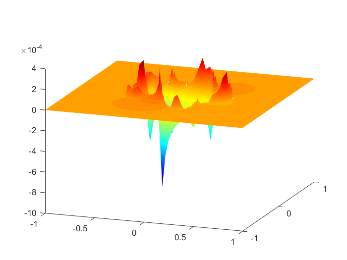
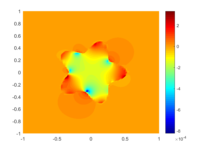
In Figures 5-6, we give the optimal discrete states $y_{h,50}^{*}$ , $y_{h,1000}^{*}$ , and the discrete co-states $p_{h,50}^{*}$ , $p_{h,1000}^{*}$ on $64\times 64$ mesh. Figure 7 demonstrates the difference $y_{h,1000}^{*}-y_{h,50}^{*}$ and $p_{h,1000}^{*}-p_{h,50}^{*}$ on $64\times 64$ mesh. These figures show that the numerical interfaces are distinct for both the state and co-state and accord with the interface of the equations. Once again we find that, a large $\widetilde{C}$ may affect the numerical results slightly.

References

[1] I. Babus̆ka. The finite element method for elliptic equations with discontinuous coefficients. Computing, 5:207–213, 1970.
[2] J.W. Barrett and C.M. Elliott. Fitted and unfitted finite-element methods for elliptic equations with smooth interfaces. IMA J. Numer. Anal., 7(3):283–300, 1987.
[3] R. Becker, E. Burman, and P. Hansbo. A Nitsche extended finite element method for incompressible elasticity with discontinuous modulus of elasticity. Comput. Methods Appl. Mech. Engrg., 198(41-44):3352–3360, 2009.
[4] R. Becker, H. Kapp, and R. Rannacher. Adaptive finite element methods for optimal control of partial differential equations: Basic concept. SIAM J. Control Optim., 39(1):113–132, 2000.
[5] T. Belytschko, R. Gracie, and G. Ventura. A review of extended/generalized finite element methods for material modeling. Modelling Simul. Mater. Sci. Eng., 17(4):1–24, 2009.
[6] O. Benedix and B. Vexler. A posteriori error estimation and adaptivity for elliptic optimal control problems with state constraints. Comput. Optim. Appl., 44(1):3–25, 2009.
[7] J.H. Bramble and J.T. King. A finite element method for interface problems in domains with smooth boundaries and interfaces. Adv. Comput. Math., 6(1):109–138, 1996.
[8] S.C. Brenner and L.R. Scott. The mathematical theory of finite element methods. Springer-Verlag, Berlin, 3rd edition, 2008.
[9] H. Brezis. Functional analysis, Sobolev space and partial differential equations. Springer, 2011.
[10] E. Burman, S. Claus, P. Hansbo, M.G. Larson, and A. Massing. Cutfem: discretizing geometry and partial differential equations. Int. J. Numer. Meth. Engng, 104(7):472–501, 2015.
[11] Z. Cai, C. He, and S. Zhang. Discontinuous finite element methods for interface problems: Robust a priori and a posteriori error estimates. SIAM J. Numer. Anal., 55(1):400–418, 2017.
[12] B. Camp, T. Lin, Y. Lin, and W. Sun. Quadratic immersed finite element spaces and their approximation capabilities. Adv. Comput. Math., 24(1-4):81–112, 2006.
[13] M. Cenanovia, P. Hansbo, and M.G. Larson. Cut finite element modeling of linear membranes. Comput. Methods Appl. Mech. Engrg., 310:98–111, 2016.
[14] Y. Chen, Y. Huang, W. Liu, and N. Yan. Error estimates and superconvergence of mixed finite elment methods for convex optimal control problems. J. Sci. Comput., 42(3):382–403, 2010.
[15] Z. Chen and J. Zou. Finite element methods and their convergence for elliptic and parabolic interface problems. Numer. Math., 79(2):175–202, 1998.
[16] B. Deka. A weak galerkin finite element method for elliptic interface problems with polynomial reduction. Numer. Math. Theor. Meth. Appl., 11:655–672, 2018.
[17] R. Fedkiw. The immersed interface method. numerical solutions of pdes involving interfaces and irregular domains. Math. Comput., 76(259):1691, 2006.
[18] W. Gong and N. Yan. Adaptive finite element method for elliptic optimal control problems: convergence and optimality. Numer. Math., 135(4):1121–1170, 2017.
[19] D. Han, P. Wang, X. He, T. Lin, and J. Wang. A 3D immersed finite element method with non-homogeneous interface flux jump for applications in particle-in-cell simulations of plasma-lunar surface interactions. J. Comput. Phys., 321:965–980, 2016.
[20] A. Hansbo and P. Hansbo. An unfitted finite element method, based on nitsche’s method, for elliptic interface problems. Comput. Methods Appl. Mech. Engrg., 191(47-48):5537–5552, 2002.
[21] P. Hansbo, M.G. Larson, and S. Zahedi. A cut finite element method for a stokes interface problem. Appl. Numer. Math., 85(C):90–114, 2014.
[22] X. He, T. Lin, and Y. Lin. Immersed finite element methods for elliptic interface problems with non-homogeneous jump conditions. Int. J. Numer. Anal. Model., 8(2):284–301, 2011.
[23] X. He, T. Lin, and Y. Lin. The convergence of the bilinear and linear immersed finite element solutions to interface problems. Numer. Methods Partial Differential Equations, 28(1):312–330, 2012.
[24] M. Hintermüller and R.H.W. Hoppe. Goal-oriented adaptivity in pointwise state constrained optimal control of partial differential equations. SIAM J. Control Optim., 48(8):5468–5487, 2010.
[25] M. Hinze. A variational discretization concept in control constrained optimization: The linear-quadratic case. Comput. Optim. Applic., 30:45–61, 2005.
[26] M. Hinze and U. Matthes. A note on variational discretization of elliptic neumann boundary control. Control Cybernet., 38(3):577–591, 2009.
[27] M. Hinze, R. Pinnau, M. Ulbrich, and S. Ulbrich. Optimization with PDE Constraints. Springer, 2009.
[28] J. Huang and J. Zou. A mortar element method for elliptic problems with discontinuous coefficients. IMA J. Numer. Anal., 22(4):549–576, 2002.
[29] D.S. Jerison and C.E. Kenig. The Neumann problem on Lipschitz domains. Bull. Am. Math. Soc., 4(2):203–207, 1981.
[30] H. Ji, Q. Zhang, Q. Wang, and Y. Xie. A partially penalised immersed finite element method for elliptic interface problems with non-homogeneous jump conditions. East. Asia. J. Appl. Math., 8:1–23, 2018.
[31] K. Kohls, K.G. Siebert, and A. Rösch. Convergence of adaptive finite elements for optimal control problems with control constraints. In G. Leugering et al., editor, Trends in PDE Constrained Optimization, volume 165 of International Series of Numerical Mathematics, pages 403–419. Birkhäuser, Cham, 2014.
[32] C. Lehrenfeld and A. Reusken. Optimal preconditioners for Nitsche-XFEM discretizations of interface problems. Numer. Math., 135(2):313–332, 2017.
[33] J. Li, M.J. Markus, B. Wohlmuth, and J. Zou. Optimal a priori estimates for higher order finite elements for elliptic interface problems. Appl. Numer. Math., 60(1-2):19–37, 2010.
[34] R. Li, W. Liu, H. Ma, and T. Tang. Adaptive finite element approximation for distributed elliptic optimal control problems. SIAM J. Control Optim., 41(5):1321–1349, 2002.
[35] Z. Li and K. Ito. The immersed interface method: numerical solutions of PDEs involving interfaces and irregular domains. Frontiers Appl. Math. 33. SIAM, Philadelphia, 2006.
[36] Z. Li, T. Lin, and X. Wu. New cartesian grid methods for interface problems using the finite element formulation. Numer. Math., 96(1):61–98, 2003.
[37] T. Lin, Y. Lin, and W. Sun. Error estimation of a class of quadratic immersed finite element methods for elliptic interface problems. Discrete Contin. Dyn. Syst. Ser. B, 7(4):807–823, 2007.
[38] T. Lin, Y. Lin, and X. Zhang. Partially penalized immersed finite element methods for elliptic interface problems. SIAM J. Numer. Anal., 53(2):1121–1144, 2015.
[39] J.L. Lions. Optimal control of systems governed by partial differential equations. Springer-Verlag, Berlin, 1971.
[40] C. Liu and C. Hu. A second order ghost fluid method for an interface problem of the poisson equation. Commun. Comput. Phys., 22(4):965–996, 2017.
[41] W. Liu, W. Gong, and N. Yan. A new finite element approximation of a state-constained optimal control problem. J. Comput. Math., 27(1):97–114, 2009.
[42] J.M. Melenk. On generalized finite element methods. PhD thesis, University of Maryland at College Park, 1995.
[43] J.M. Melenk and I. Babus̆ka. The partition of unity finite element method: basic theory and applications. Comput. Methods Appl. Mech. Engrg., 139(1-4):289–314, 1996.
[44] N. Moës, J. Dolbow, and T. Belytschko. A finite element method for crack growth without remeshing. Int. J. Numer. Meth. Engng., 46(1):131–150, 1999.
[45] J. Nitsche. Über ein variationsprinzip zur lösung von dirichlet-problemen bei verwendungvon von teilräumen, die keinen randbedingungen unterworfen sind. Abh. Math. Univ. Hamburg, 36(1):9–15, 1971.
[46] M. Plum and C. Wieners. Optimal a priori estimates for interface problems. Numer. Math., 95(4):735–759, 2003.
[47] A. Rösch, K.G. Siebert, and S. Steinig. Reliable a posteriori error estimation for state-constrained optimal control. Comput. Optim. Appl., 68(1):121–162, 2017.
[48] R. Schneider and G. Wachsmuth. A posteriori error estimation for control-constrained, linear-quadratic optimal control problems. SIAM J. Numer. Anal., 54(2):1169–1192, 2016.
[49] B. Schott. Stabilized cut finite element methods for complex interface coupled flow problems. PhD thesis, Technische Universität München, 2017.
[50] L.R. Scott and S. Zhang. Finite element interpolation of nonsmooth functions satisfying boundary conditions. Math. Comp., 54(190):483–493, 1990.
[51] T. Strouboulis, I. Babus̆ka, and K. Copps. The design and analysis of the generalized finite element method. Comput. Methods Appl. Mech. Engrg., 181(1):43–69, 2000.
[52] F. Tröltzsch. Optimal control of partial differential equations: Theory,method and applications, volume 112 of Graduate studies in mathematics. American mathematical society, Providence, Rhode Island, 2010.
[53] D. Wachsmuth and J.E. Wurst. Optimal control of interface problems with hp-finite elements. Nume. Funct. Anal. Optim., 37(3):363–390, 2016.
[54] Z. Weng, J.Z. Yang, and X. Lu. A stabilized finite element method for the convection dominated diffusion optimal control problem. Appl. Anal., 95(12):2807–2823, 2016.
[55] J. Xu. Estimate of the convergence rate of the finite element solutions to elliptic equation of second order with discontinuous coefficients. Natural Science Journal of Xiangtan University, 1:84–88, 1982. (in Chinese).
[56] J. Xu and S. Zhang. Optimal finite element methods for interface problems. In T. Dickopf et al., editor, Domain Decomposition Methods in Science and Engineering XXII, volume 104 of Lecture Notes in Computational Science and Engineering, pages 77–91. Springer, Cham, 2016.
[57] F.W. Yang, C. Venkataraman, V. Styles, and A. Madzvamuse. A robust and efficient adaptive multigrid solver for the optimal control of phase field formulations of geometric evolution laws. Commun. Comput. Phys., 21(1):65–92, 2017.
[58] Q. Zhang, K. Ito, Z. Li, and Z. Zhang. Immersed finite elements for optimal control problems of elliptic pdes with interfaces. J. Comput. Phys., 298(C):305–319, 2015.
[59] H. Zhu, K. Liang, G. He, and J. Ying. A splitting collocation method for elliptic interface problems. Numer. Math. Theor. Meth. Appl., 11:491–505, 2018.

	$\displaystyle\\|[w-I_{h}^{*}w]\\|_{\frac{1}{2},h,\Gamma}^{2}$	$\displaystyle\lesssim\sum_{i=1}^{2}\sum_{K\in G_{h}}h_{K}^{-1}\\|w_{i}-I_{h}E_{i}w_{i}\\|_{0,\Gamma_{K}}^{2}=\sum_{i=1}^{2}\sum_{K\in G_{h}}h_{K}^{-1}\\|E_{i}w_{i}-I_{h}E_{i}w_{i}\\|_{0,\Gamma_{K}}^{2}$
		$\displaystyle\lesssim\sum_{i=1}^{2}\sum_{K\in G_{h}}(h_{K}^{-2}\\|E_{i}w_{i}-I_{h}E_{i}w_{i}\\|_{0,K}^{2}+\\|E_{i}w_{i}-I_{h}E_{i}w_{i}\\|_{1,K}^{2})$
		$\displaystyle\lesssim\sum_{i=1}^{2}\sum_{K\in G_{h}}h_{K}\\|E_{i}w_{i}\\|_{\frac{3}{2},S_{K}}^{2}$
		$\displaystyle\lesssim\sum_{i=1}^{2}h\\|E_{i}w_{i}\\|_{\frac{3}{2},\Omega}^{2}\lesssim\sum_{i=1}^{2}h\\|w_{i}\\|_{\frac{3}{2},\Omega_{i}}^{2}\lesssim h\\|w\\|_{\frac{3}{2},\Omega_{1}\cup\Omega_{2}}^{2}.$

	$\displaystyle\\|\{\nabla_{n}(w-I_{h}^{*}w)\}\\|_{-\frac{1}{2},h,\Gamma}^{2}$	$\displaystyle\lesssim\sum_{i=1}^{2}\sum_{K\in G_{h}}h_{K}\\|\nabla_{n}(w_{i}-I_{h}E_{i}w_{i})\\|_{0,\Gamma_{K}}^{2}$
		$\displaystyle\lesssim\sum_{i=1}^{2}\sum_{K\in G_{h}}h_{K}\\|E_{i}w_{i}\\|_{\frac{3}{2},K}^{2}$
		$\displaystyle\lesssim\sum_{i=1}^{2}h\\|E_{i}w_{i}\\|_{\frac{3}{2},\Omega}^{2}\lesssim\sum_{i=1}^{2}h\\|w_{i}\\|_{\frac{3}{2},\Omega_{i}}^{2}\lesssim h\\|w\\|_{\frac{3}{2},\Omega_{1}\cup\Omega_{2}}^{2}.$

	$\displaystyle\|\|\|z-z_{h}\|\|\|$	$\displaystyle\lesssim h^{\frac{1}{2}}\\|z\\|_{\frac{3}{2},\Omega_{1}\cup\Omega_{2}}$
		$\displaystyle\lesssim h^{\frac{1}{2}}\\|y^{*}-y^{h}\\|_{0,\Omega}.$		(3.25)

	$\displaystyle\|\|\|z-z_{h}\|\|\|$	$\displaystyle\lesssim h^{\frac{1}{2}}\\|z\\|_{\frac{3}{2},\Omega_{1}\cup\Omega_{2}}$
		$\displaystyle\lesssim h^{\frac{1}{2}}\\|y^{*}-(\kappa_{2}y^{h}_{1}+\kappa_{1}y^{h}_{2})\\|_{0,\Gamma}.$		(3.32)

$\displaystyle\sqrt{\alpha}\\|u^{}-u_{h}^{}\\|_{0,\Gamma}+\\|y^{}-y_{h}^{}\\|_{0,\Omega}\leq$	$\displaystyle\sqrt{2}\\|y^{}-y^{h}\\|_{0,\Omega}+\frac{\sqrt{2}}{\sqrt{\alpha}}\\|p^{}-(\kappa_{2}p^{h}_{1}+\kappa_{1}p^{h}_{2})\\|_{0,\Gamma}$	(4.6)
$\displaystyle\\|p^{}-p_{h}^{}\\|_{0,\Omega}\lesssim$	$\displaystyle\\|p^{}-p^{h}\\|_{0,\Omega}+\\|y^{}-y_{h}^{*}\\|_{0,\Omega}$	(4.7)
$\displaystyle\|\|\|y^{}-y_{h}^{}\|\|\|\lesssim$	$\displaystyle\|\|\|y^{}-y^{h}\|\|\|+\\|u^{}-u_{h}^{*}\\|_{0,\Gamma}$	(4.8)
$\displaystyle\|\|\|p^{*}-p_{h}\|\|\|\lesssim$	$\displaystyle\|\|\|p^{}-p^{h}\|\|\|+\\|y^{}-y_{h}^{*}\\|_{0,\Omega}.$	(4.9)