Integral equation methods for electrostatics, acoustics and electromagnetics in smoothly varying, anisotropic media

This work was supported in part by the Spanish Ministry of Science and Innovation under project TEC2016-78028-C3-3-P and the U.S. Department of Energy under grant DE-FG02-86ER53223.

Lise-Marie Imbert-Gerard Note: Department of Mathematics, University of Maryland. Email: lmig@math.umd.edu Felipe Vico Note: Instituto de Telecomunicaciones y Aplicaciones Multimedia (ITEAM), Universidad Politècnica de València, 46022 València, Spain. email: felipe.vico@gmail.com, mferrand@dcom.upv.es Leslie Greengard Note: Courant Institute, New York University, and Flatiron Institute, Simons Foundation, New York, NY. Email: greengard@cims.nyu.edu Miguel Ferrando³³footnotemark: 3

Abstract

We present a collection of well-conditioned integral equation methods for the solution of electrostatic, acoustic or electromagnetic scattering problems involving anisotropic, inhomogeneous media. In the electromagnetic case, our approach involves a minor modification of a classical formulation. In the electrostatic or acoustic setting, we introduce a new vector partial differential equation, from which the desired solution is easily obtained. It is the vector equation for which we derive a well-conditioned integral equation. In addition to providing a unified framework for these solvers, we illustrate their performance using iterative solution methods coupled with the FFT-based technique of [1] to discretize and apply the relevant integral operators.

1 Introduction

In this paper, we develop fast, high order accurate integral equation methods for several classes of elliptic partial differential equations (PDEs) in three dimensions involving anisotropic, inhomogeneous media. In the electrostatic setting, we consider the anisotropic Laplace equation

\displaystyle\nabla\cdot\epsilon(\boldsymbol{x})\nabla\phi(\boldsymbol{x})=0,\ \ \boldsymbol{x}\in\mathbb{R}^{3}\,,

(1)

where $\epsilon(\boldsymbol{x})$ is a real, $3\times 3$ symmetric matrix, subject to certain regularity conditions discussed below. We also assume $\epsilon(\boldsymbol{x})$ is a compact perturbation of the identity operator $I$ - that is, $\epsilon(\boldsymbol{x})-I$ has compact support. A typical objective is to determine the response of the inclusion to a known, applied static field, with the response satisfying suitable decay conditions at infinity.

For acoustic or electromagnetic modeling in the frequency domain, we consider the anisotropic Helmholtz equation

\displaystyle\nabla\cdot\epsilon^{-1}(\boldsymbol{x})\nabla\phi(\boldsymbol{x})+\omega^{2}\phi(\boldsymbol{x})=0,\ \ \boldsymbol{x}\in\mathbb{R}^{3}

(2)

and the anisotropic Maxwell equations

	$\displaystyle\nabla\times\boldsymbol{E}(\boldsymbol{x})$	$\displaystyle=i\omega\mu(\boldsymbol{x})\boldsymbol{H}(\boldsymbol{x})$		(3)
	$\displaystyle\nabla\times\boldsymbol{H}(\boldsymbol{x})$	$\displaystyle=-i\omega\epsilon(\boldsymbol{x})\boldsymbol{E}(\boldsymbol{x}),\ \ \ \ \ \ \ \ \boldsymbol{x}\in\mathbb{R}^{3},$		(3)

respectively. Here, $\epsilon(\boldsymbol{x})$ and $\mu(\boldsymbol{x})$ are complex-valued $3\times 3$ matrices, subject to regularity and spectral properties to be discussed in detail. We again assume that $\epsilon(\boldsymbol{x})$ and $\mu(\boldsymbol{x})$ are compact perturbation of the identity. A typical objective is to determine the response of the inclusion to an impinging acoustic or electromagnetic wave, with the response satisfying suitable radiation conditions at infinity. For a thorough discussion of the origins and applications of these problems, we refer the reader to the textbooks [2, 3, 4].

Instead of discretizing the partial differential equations (PDEs) themselves, we will develop integral representations of the solution that satisfy the outgoing decay/radiation conditions exactly, avoiding the need for truncating the computational domain and imposing approximate outgoing boundary conditions. The resulting integral equations will be shown to involve equations governed by operators of the form $I+B+K$ where $I$ is the identity, $B$ is a linear contraction mapping, $K$ is compact. A simple argument based on the Neumann series will allow us to extend the Fredholm alternative to this setting (and therefore to prove existence for the original, anisotropic, elliptic PDEs themselves). Moreover, our formulations permit high-order accurate discretization, and FFT-based acceleration on uniform grids. In the electromagnetic case, our approach is closely related to some classical formulations. For the Laplace and Helmholtz equations, however, our approach appears to be new and depends on the construction of a vector PDE from which the desired solution is easily obtained. It is the vector PDE for which we will derive a new, well-conditioned integral equation. One purpose of the present paper is to describe all of these solvers in a unified framework. Given that resonance-free second kind integral equations are typically well-conditioned, they are suitable for solution using simple iterative methods such as GMRES and BICGSTAB without any preconditioner. We use the method of [1] to discretize and apply the integral operators with high order accuracy and demonstrate the performance of our scheme with several numerical examples.

We will use the language of scattering theory throughout. Thus, for the scalar equations, we write $\phi=\phi^{\operatorname{inc}}+\phi^{\operatorname{scat}}$ where $\phi^{\operatorname{inc}}$ is a known function that satisfies the homogeneous, isotropic Laplace or Helmholtz equation in free space away from sources. In the electrostatic case, $\phi^{\operatorname{scat}}$ is assumed to satisfy the decay condition

\lim_{r\rightarrow\infty}\phi^{\operatorname{scat}}=o(1),

(4)

where $r=|\boldsymbol{x}|$ . In the acoustic case [5], $\phi^{\operatorname{scat}}$ is assumed to satisfy the Sommerfeld radiation condition

\lim_{r\rightarrow\infty}r\left(\frac{\partial\phi^{\operatorname{scat}}}{\partial r}-i\omega\phi^{\operatorname{scat}}\right)=0.

(5)

In the electromagnetic setting (3), we write $\boldsymbol{E}=\boldsymbol{E}^{\operatorname{inc}}+\boldsymbol{E}^{\operatorname{scat}}$ and $\boldsymbol{H}=\boldsymbol{H}^{\operatorname{inc}}+\boldsymbol{H}^{\operatorname{scat}}$ , with $\boldsymbol{E}^{\operatorname{inc}},\boldsymbol{H}^{\operatorname{inc}}$ corresponding to a known solution of the homogeneous, isotropic Maxwell equations in free space away from sources. $\boldsymbol{E}^{\operatorname{scat}},\boldsymbol{H}^{\operatorname{scat}}$ are assumed to satisfy the Silver-Müller radiation condition [5]:

\lim_{r\rightarrow\infty}\left(\boldsymbol{H}^{\operatorname{scat}}\times{\boldsymbol{x}}-r\boldsymbol{E}^{\operatorname{scat}}\right)=0.

(6)

2 The anisotropic Laplace equation

We first consider the electrostatic problem (1), where $\epsilon(\boldsymbol{x})$ is a real, symmetric, positive definite $3\times 3$ matrix with bounded entries, such that $\epsilon(\boldsymbol{x})-I$ has compact support. We assume that the smallest eigenvalue of $\epsilon(\boldsymbol{x})$ is bounded away from zero, so that the PDE is uniformly elliptic (see [6], p.294).

Letting $\phi=\phi^{\operatorname{inc}}+\phi^{\operatorname{scat}}$ , we assume that $\phi^{\operatorname{inc}}(\boldsymbol{x})$ is a given “applied field” with $\Delta\phi^{\operatorname{inc}}(\boldsymbol{x})=0$ in the support of $\epsilon(\boldsymbol{x})-I$ .

Definition 1.

By the anisotropic electrostatic scattering problem (or simply the electrostatic scattering problem) we mean the calculation of a function $\phi^{\operatorname{scat}}(\boldsymbol{x})\in H^{1}_{loc}(\mathbb{R}^{3})$ that satisfies the radiation condition (4) and the equation

\displaystyle\nabla\cdot\epsilon(\boldsymbol{x})\nabla\phi^{\operatorname{scat}}(\boldsymbol{x})=-\nabla\cdot(\epsilon(\boldsymbol{x})-I)\nabla\phi^{\operatorname{inc}}(\boldsymbol{x})

(7)

for $\boldsymbol{x}\in\mathbb{R}^{3}$ . Given this function $\phi^{\operatorname{scat}}$ , $\phi=\phi^{\operatorname{inc}}+\phi^{\operatorname{scat}}$ clearly satisfies the eq. (1).

Because of the mild regularity assumptions made on $\epsilon(\boldsymbol{x})$ and on the solution $\phi^{\operatorname{scat}}$ , we must interpret eq. (7) in a weak sense (eq. (8) below).

We begin by proving a uniqueness result.

Theorem 1.

The anisotropic electrostatic scattering problem has at most one solution.

Proof.

Let $B_{R}$ be an open ball centered at the origin that contains the support of $\epsilon(\boldsymbol{x})-I$ , and let $T$ denote the Dirichlet-to-Neumann (DtN) map for harmonic functions in the exterior of $B_{R}$ . Integrating (7) by parts, we obtain the weak formulation on $B_{R}$ :

\int_{B_{R}}\nabla\psi(\boldsymbol{x})\epsilon(\boldsymbol{x})\nabla\phi^{\operatorname{scat}}(\boldsymbol{x})dV=\int_{\partial B_{R}}\psi T[\phi^{\operatorname{scat}}]dS-\int_{B_{R}}\nabla\psi(\boldsymbol{x})(\epsilon-I)(\boldsymbol{x})\nabla\phi^{\operatorname{inc}}(\boldsymbol{x})dV

(8)

for $\psi\in H^{1}(B_{R})$ . Assuming no “incoming” data ( $\phi^{\operatorname{inc}}=0$ ) and using $\psi=\phi^{\operatorname{scat}}$ itself as a testing function yields

\int_{B_{R}}\nabla\phi^{\operatorname{scat}}(\boldsymbol{x})\epsilon(\boldsymbol{x})\nabla\phi^{\operatorname{scat}}(\boldsymbol{x})dV=\int_{\partial B_{R}}\phi^{\operatorname{scat}}T[\phi^{\operatorname{scat}}]dS.

(9)

From the uniform ellipticity of $\epsilon(\boldsymbol{x})$ , for some constant $C>0$ we have

C\int_{B_{R}}|\nabla\phi^{\operatorname{scat}}(\boldsymbol{x})|^{2}dV\leq\int_{\partial B_{R}}\phi^{\operatorname{scat}}T[\phi^{\operatorname{scat}}]dS.

(10)

On the surface of $B_{R}$ , the DtN map can be computed in the spherical harmonics basis, with

T[Y_{nm}](\theta,\phi)=-(n+1)Y_{nm}(\theta,\phi).

From this, it is straightforward to see that

\int_{B_{R}}|\nabla\phi^{\operatorname{scat}}(\boldsymbol{x})|^{2}dV=0\Rightarrow\phi^{\operatorname{scat}}(\boldsymbol{x})=c\ \forall\boldsymbol{x}\in B_{R}.

(11)

Using (10), we have

0\leq\int_{\partial B_{R}}\phi^{\operatorname{scat}}T[\phi^{\operatorname{scat}}]dS=\int_{\partial B_{R}}cT[c]dS=-|c|^{2}A,

(12)

where $A$ is the surface area of $B_{R}$ . Thus, $c=0$ , yielding the desired result. ∎

Remark 1.

While the standard proof of existence for the anisotropic Laplace equation relies on the Lax-Milgram theorem [6], we turn now to an alternate approach, based on deriving an auxiliary vector PDE and a corresponding, well-conditioned, Fredholm integral equation.

Note first that eq. (7) can be rewritten in the form

\nabla\cdot\epsilon\nabla\phi^{\operatorname{scat}}=\Delta\phi^{\operatorname{scat}}+\nabla\cdot(\epsilon-I)\nabla\phi^{\operatorname{scat}}=-\nabla\cdot\epsilon\nabla\phi^{\operatorname{inc}}=-\nabla\cdot(\epsilon-I)\nabla\phi^{\operatorname{inc}},

(13)

since $\phi^{\operatorname{inc}}$ is harmonic in $B_{R}$ , a region which contains the support of $\epsilon(\boldsymbol{x})-I$ . Recall that $\phi^{\operatorname{scat}}$ satisfies the Laplace decay condition (4).

Suppose now that $\boldsymbol{F}$ is a vector field such that $\nabla\cdot\boldsymbol{F}=\phi^{\operatorname{scat}}$ and satisfies (4). Note, however, that $\nabla\times\boldsymbol{F}$ is, as yet, unspecified. Then, $\boldsymbol{F}$ satisfies the following equation:

\Delta\nabla\cdot\boldsymbol{F}+\nabla\cdot(\epsilon-I)\nabla\nabla\cdot\boldsymbol{F}=-\nabla\cdot(\epsilon-I)\nabla\phi^{\operatorname{inc}},

(14)

\nabla\cdot\Delta\boldsymbol{F}+\nabla\cdot(\epsilon-I)\nabla\nabla\cdot\boldsymbol{F}=-\nabla\cdot(\epsilon-I)\nabla\phi^{\operatorname{inc}}.

(15)

We now define the auxiliary equation for $\boldsymbol{F}$ (which will determine its curl):

\Delta\boldsymbol{F}+(\epsilon-I)\nabla\nabla\cdot\boldsymbol{F}=-(\epsilon-I)\nabla\phi^{\operatorname{inc}}\,.

(16)

Since eq. (15) is obtained by taking the divergence of (16), it is natural to introduce the following definition.

Definition 2.

By the vector electrostatic scattering problem we mean the calculation of a vector function $\mathbf{F}^{\operatorname{scat}}(\boldsymbol{x})\in H^{2}_{loc}(\mathbb{R}^{3})$ that satisfies

\displaystyle\Delta\mathbf{F}^{\operatorname{scat}}+(\epsilon-I)\nabla\nabla\cdot\mathbf{F}^{\operatorname{scat}}=-(\epsilon-I)\nabla\nabla\cdot\mathbf{F}^{\operatorname{inc}}

(17)

and the standard decay condition at infinity:

\displaystyle\mathbf{F}^{\operatorname{scat}}(\boldsymbol{x})=o(1),\ \ {\rm as}\ |\boldsymbol{x}|\rightarrow\infty,

(18)

uniformly in all directions. Here, $\mathbf{F}^{\operatorname{inc}}(\boldsymbol{x})$ is an $H^{2}$ function defined on an open set that contains the support of $\epsilon(\boldsymbol{x})-I$ , where it satisfies $\Delta\mathbf{F}^{\operatorname{inc}}(\boldsymbol{x})=0$ .

Due to the regularity properties imposed on $\mathbf{F}^{\operatorname{scat}}$ and the lack of derivatives acting on the entries of $\epsilon_{ij}(\boldsymbol{x})$ , eq. (18) does not need to be interpreted in a weak sense. We now establish a relation between the vector and scalar problems.

Lemma 1.

If $\mathbf{F}^{\operatorname{scat}}(\boldsymbol{x})\in H^{2}_{loc}(\mathbb{R}^{3})$ satisfied the vector electrostatic scattering problem, then $\phi^{\operatorname{scat}}(\boldsymbol{x}):=\nabla\cdot\mathbf{F}^{\operatorname{scat}}(\boldsymbol{x})\in H^{1}_{loc}(\mathbb{R}^{3})$ and satisfies the anisotropic electrostatic scattering problem with right hand side given by the incoming field $\phi^{\operatorname{inc}}=\nabla\cdot\mathbf{F^{\operatorname{inc}}}$ .

Proof.

If we assume that $\mathbf{F}^{\operatorname{scat}}(\boldsymbol{x})\in H^{3}_{loc}(\mathbb{R}^{3})$ , then the result follows immediately by taking the divergence of eq. (17) and interchange the order of the operators. In general, however, we cannot assume such regularity for $\mathbf{F}^{\operatorname{scat}}(\boldsymbol{x})$ , in particular if there are discontinuities in the entries $\epsilon(\boldsymbol{x})_{ij}$ .

Thus, for the general case, we let $B_{R}$ be an open ball centered at the origin that contains the support of $\epsilon(\boldsymbol{x})-I$ . In the region $\mathbb{R}^{3}\backslash B_{R}$ , the governing differential operator is the isotropic Laplacian $\Delta$ and, by standard regularity results (see, for example, Corollary 8.11 in [7]), the solution $\mathbf{F}_{i}^{\operatorname{scat}}\in C^{\infty}$ . Thus, we can interpret the radiation condition in the strong sense. We can now apply the representation theorems 4.11 and 4.13 from [5] in the region $\mathbb{R}^{3}\backslash B_{R}$ , in the limit $k=0$ . From this, it follows that $\nabla\cdot\boldsymbol{F}^{\operatorname{scat}}=O\left(\frac{1}{|\boldsymbol{x}|^{2}}\right)$ uniformly in all directions. Thus, $\phi^{\operatorname{scat}}(\boldsymbol{x})=\nabla\cdot\boldsymbol{F}^{\operatorname{scat}}$ satisfies the radiation condition (4) for the anisotropic electrostatic scattering problem.

Let $\psi\in H^{1}(B_{R})$ . From eq. (17), we can write

\displaystyle\nabla\psi\cdot\Big(\Delta\mathbf{F}^{\operatorname{scat}}+(\epsilon-I)\nabla\nabla\cdot\mathbf{F}^{\operatorname{scat}}\Big)=-\nabla\psi(\boldsymbol{x})\cdot(\epsilon-I)\nabla\nabla\cdot\mathbf{F}^{\operatorname{inc}}.

(19)

Using the vector identity $\Delta\mathbf{F}^{\operatorname{scat}}=-\nabla\times\nabla\times\mathbf{F}^{\operatorname{scat}}+\nabla\nabla\cdot\mathbf{F}^{\operatorname{scat}}$ , we have

\displaystyle-\nabla\psi\cdot\nabla\times\nabla\times\mathbf{F}^{\operatorname{scat}}+\nabla\psi\cdot\epsilon\nabla\nabla\cdot\mathbf{F}^{\operatorname{scat}}=-\nabla\psi\cdot(\epsilon-I)\nabla\nabla\cdot\mathbf{F}^{\operatorname{inc}}.

(20)

Integrating over the ball $B_{R}$ , we obtain

	$\displaystyle\int_{B_{R}}-\nabla\psi\cdot\nabla\times\nabla\times\mathbf{F}^{\operatorname{scat}}dV+$	$\displaystyle\int_{B_{R}}\nabla\psi\cdot\epsilon\nabla\nabla\cdot\mathbf{F}^{\operatorname{scat}}dV=$		(21)
	$\displaystyle-$	$\displaystyle\int_{B_{R}}\nabla\psi\cdot(\epsilon-I)\nabla\nabla\cdot\mathbf{F}^{\operatorname{inc}}dV.$		(21)

We will make use of the following identity that holds for every function $\mathbf{F}\in H^{2}(B_{R})$ , $\psi\in H^{1}(B_{R})$ and is straightforward to derive from the divergence theorem:

\displaystyle\int_{B_{R}}\nabla\psi\cdot\nabla\times\nabla\times\mathbf{F}dV=\int_{\partial B_{R}}\psi\boldsymbol{n}\cdot\nabla\times\nabla\times\mathbf{F}dS.

(22)

Combining (22) and (21), we obtain

	$\displaystyle\int_{B_{R}}\nabla\psi\cdot\epsilon\nabla\nabla\cdot\mathbf{F}^{\operatorname{scat}}dV$	$\displaystyle=\int_{\partial B_{R}}\psi\boldsymbol{n}\cdot\nabla\times\nabla\times\mathbf{F}^{\operatorname{scat}}dV$		(23)
	$\displaystyle-$	$\displaystyle\int_{B_{R}}\nabla\psi\cdot(\epsilon-I)\nabla\nabla\cdot\mathbf{F}^{\operatorname{inc}}dV.$		(23)

Since $\Delta\mathbf{F}^{\operatorname{scat}}(\boldsymbol{x})=0$ for $\boldsymbol{x}\in\partial B_{R}$ , we may write

\int_{\partial B_{R}}\psi\boldsymbol{n}\cdot\nabla\times\nabla\times\mathbf{F}^{\operatorname{scat}}dV=\int_{\partial B_{R}}\psi\boldsymbol{n}\cdot\nabla\nabla\cdot\mathbf{F}^{\operatorname{scat}}dV.

(24)

Thus,

\displaystyle\int_{B_{R}}\nabla\psi(\boldsymbol{x})\cdot\epsilon\nabla\nabla\cdot\mathbf{F}^{\operatorname{scat}}dV=\int_{\partial B_{R}}\psi T[\nabla\cdot\mathbf{F}^{\operatorname{scat}}]dS-\int_{B_{R}}\nabla\psi(\boldsymbol{x})\cdot(\epsilon-I)\nabla\nabla\cdot\mathbf{F}^{\operatorname{inc}}dV.

(25)

In short, for $\phi^{\operatorname{inc}}:=\nabla\cdot\mathbf{F}^{\operatorname{inc}}$ , $\phi^{\operatorname{scat}}:=\nabla\cdot\mathbf{F}^{\operatorname{scat}}$ satisfes (8), the weak version of the anisotropic electrostatic scattering problem. ∎

Theorem 2 (Uniqueness).

The vector electrostatic scattering problem has at most one solution.

Proof.

Let $\boldsymbol{F}^{\operatorname{scat}}\in H^{2}_{loc}(\mathbb{R}^{3})$ be a solution of the homogeneous equation

\Delta\boldsymbol{F}^{\operatorname{scat}}+(\epsilon-I)\nabla\nabla\cdot\boldsymbol{F}^{\operatorname{scat}}=0

(26)

that satisfies the radiation condition. By Lemma 1, $\nabla\cdot\mathbf{F}^{\operatorname{scat}}$ satisfies the homogeneous weak formulation (8) and, as a consequence, using Theorem 1, $\nabla\cdot\mathbf{F}^{\operatorname{scat}}=0$ . From eq. (26), it then follows that $\Delta\mathbf{F}^{\operatorname{scat}}(\boldsymbol{x})=0$ for all $\boldsymbol{x}\in\mathbb{R}^{3}$ , so that $\mathbf{F}^{\operatorname{scat}}=0$ for all $\boldsymbol{x}\in\mathbb{R}^{3}$ . ∎

We turn now to the question of existence, for which we define the volume integral operator

\mathcal{V}_{0}(\boldsymbol{J}):=\int_{\mathbb{R}^{3}}\frac{1}{4\pi|\boldsymbol{x}-\boldsymbol{y}|}\boldsymbol{J}(\boldsymbol{y})dV_{\boldsymbol{y}}.

(27)

It is well-known (see, for example, Theorem 8.2 in [8]) that $\mathcal{V}_{0}:L^{2}(\Omega)\rightarrow H^{2}(\Omega)$ is a continuous map for any bounded open set $\Omega\subset\mathbb{R}^{3}$ and that

\displaystyle\Delta\mathcal{V}_{0}(\boldsymbol{J})

\displaystyle=-\boldsymbol{J}.

(28)

We define the operator $\mathcal{T}_{0}$ by

\mathcal{T}_{0}(\boldsymbol{J}):=\frac{\boldsymbol{J}}{2}+\nabla\nabla\cdot\mathcal{V}_{0}(\boldsymbol{J}).

(29)

Lemma 2.

Let $H_{\epsilon}$ denote the operator mapping $L^{2}(\mathbb{R}^{3})\rightarrow L^{2}(\mathbb{R}^{3})$ with

H_{\epsilon}(\boldsymbol{x})\boldsymbol{J}(\boldsymbol{x})=(\epsilon(\boldsymbol{x})+I)^{-1}(\epsilon(\boldsymbol{x})-I)\boldsymbol{J}(\boldsymbol{x}).

(30)

Then, $\|H_{\epsilon}(\boldsymbol{x})\|_{2}<1$ .

Proof.

For $z\in\mathbb{C}$ , let $f(z)=\frac{z-1}{z+1}$ . $f$ maps the open half space $\Re{z}>0$ to $|f(z)|<1$ . Since $\epsilon(\boldsymbol{x})$ is assumed to be real symmetric and uniformly elliptic, it is expressible in diagonal form as $\epsilon(\boldsymbol{x})=U(\boldsymbol{x})D(\boldsymbol{x})U^{*}(\boldsymbol{x})$ , with the diagonal elements of $D(\boldsymbol{x})$ positive and bounded away from zero [6]. It follows that $\rho_{\epsilon}(\boldsymbol{x})=U(\boldsymbol{x})f(D)(\boldsymbol{x})U^{*}(\boldsymbol{x})\in L^{\infty}(\mathbb{R}^{3})$ , with eigenvalues strictly bounded by one, proving the desired result. ∎

Lemma 3.

The operator $2\mathcal{T}_{0}(\boldsymbol{J})$ is an isometry on $L^{2}(\mathbb{R}^{3})$ . That is, $\|2\mathcal{T}_{0}\|_{L^{2}(\mathbb{R}^{3})}=1.$

Proof.

Using the Helmholtz decomposition (see, for example, Theorem 14 in [9]), we can write $\boldsymbol{J}=\nabla\psi+\nabla\times\mathbf{P}$ . It is straightforward to check that $2\mathcal{T}_{0}(\nabla\times\mathbf{P})=\nabla\times\mathbf{P}$ , while $2\mathcal{T}_{0}(\nabla\phi)=-\nabla\phi$ . Thus, $2\mathcal{T}_{0}(\boldsymbol{J})=-\nabla\psi+\nabla\times\mathbf{P}$ and the result follows immediately from the orthogonality of the Helmholtz decomposition. ∎

Theorem 3.

There exist solutions to the anisotropic scalar and vector electrostatic scattering problems.

Proof.

We note first that the vector field $\boldsymbol{F}:=\mathcal{V}_{0}(\boldsymbol{J})$ satisfies eq. (16) if and only if $\boldsymbol{J}$ satisfies

-\boldsymbol{J}+(\epsilon-I)\nabla\nabla\cdot\mathcal{V}_{0}(\boldsymbol{J})=-(\epsilon-I)\nabla\phi^{\operatorname{inc}}.

(31)

From (29), this is equivalent to

-\boldsymbol{J}+(\epsilon-I)\Big(-\frac{\boldsymbol{J}}{2}+\mathcal{T}_{0}(\boldsymbol{J})\Big)=-(\epsilon-I)\nabla\phi^{\operatorname{inc}}.

(32)

Multiplying by $-2(\epsilon+I)^{-1}$ and a little algebra yields

(I+B)\boldsymbol{J}=2H_{\epsilon}\nabla\phi^{\operatorname{inc}},

(33)

where $H_{\epsilon}$ is defined in (30) and $B(\boldsymbol{J}):=-2H_{\epsilon}\mathcal{T}_{0}(\boldsymbol{J})$ . Eq. (33) is an integral equation for $\boldsymbol{J}$ . Moreover, from Lemmas 2 and 3, the operator $B:L^{2}(B_{R})\rightarrow L^{2}(B_{R})$ satisfies $\|B\|<1$ , so that $(I+B)$ is invertible using the Neumann series:

\boldsymbol{J}=2(I+B)^{-1}H_{\epsilon}\nabla\phi^{\operatorname{inc}}=2\sum_{n=0}^{\infty}B^{n}H_{\epsilon}\nabla\phi^{\operatorname{inc}}.

Since the volume integral operator $\mathcal{V}_{0}$ maps $L^{2}(B_{R})$ to $H^{2}(B_{R})$ , it follows that $\mathbf{F}:=\mathcal{V}_{0}(\boldsymbol{J})\in H^{2}_{loc}(\mathbb{R}^{3})$ . Thus, $\mathbf{F}$ is a solution to the vector electrostatic scattering problem, and $\nabla\cdot\mathbf{F}\in H^{1}_{loc}(\mathbb{R}^{3})$ is a solution to the anisotropic electrostatic scattering problem. ∎

The same result holds in the two-dimensional case.

Remark 2 (Smoothness of the coefficients).

From a practical viewpoint, the integral equation (33) can be discretized using a Nyström method and solved iteratively to obtain a numerical solution of the original scalar problem (7). It is worth noting that no estimate involving derivatives of $\epsilon_{ij}(\boldsymbol{x})$ is required. Because it is a Fredholm equation of the second kind, the order of accuracy obtained in the solution is the same as the order of accuracy used in the underlying quadrature rule [10]. Of course, if there are jumps in $\epsilon(\boldsymbol{x})$ , then adaptive discretization methods are recommended for resolution, but additional unknowns and surface integral operators are not required to account for the effect of these discontinuities.

3 The anisotropic Helmholtz equation

In this section, we assume that the matrix $\epsilon(\boldsymbol{x})$ has entries in $C^{1}(\mathbb{R}^{3})$ , although we will discuss some of the issues raised in relaxing this assumption. We will also assume that $\epsilon(\boldsymbol{x})$ can be diagonalized in the form

\epsilon(\boldsymbol{x})=U(\boldsymbol{x})D(\boldsymbol{x})U^{*}(\boldsymbol{x}),

where $U(\boldsymbol{x})$ is a unitary complex matrix and $D(\boldsymbol{x})$ is a diagonal matrix with positive definite real part (with entries bounded away from zero) and a positive semi-definite imaginary part (see [11]). We will also assume that $\epsilon(\boldsymbol{x})-I$ has compact support, where $I$ is the $3\times 3$ identity matrix. After proving uniqueness for the anisotropic Helmholtz equation, we introduce a related vector Helmholtz equation that will be used to establish existence using Fredholm theory.

Definition 3.

By the anisotropic Helmholtz scattering problem, we mean the determination of a function $\phi^{\operatorname{scat}}(\boldsymbol{x})\in H^{1}_{loc}(\mathbb{R}^{3})$ that satisfies the equation:

\displaystyle\nabla\cdot\epsilon^{-1}(\boldsymbol{x})\nabla\phi^{\operatorname{scat}}(\boldsymbol{x})+\omega^{2}\phi^{\operatorname{scat}}(\boldsymbol{x})=-\nabla\cdot(\epsilon^{-1}(\boldsymbol{x})-I)\nabla\phi^{\operatorname{inc}},\ \ \boldsymbol{x}\in\mathbb{R}^{3},

(34)

where $\phi^{\operatorname{inc}}$ is a known function with

\Delta\phi^{\operatorname{inc}}(\boldsymbol{x})+\omega^{2}\phi^{\operatorname{inc}}(\boldsymbol{x})=0

in the support of $\epsilon(\boldsymbol{x})-I$ . $\phi^{\operatorname{scat}}(\boldsymbol{x})$ must also satisfy the Sommerfeld radiation condition (5).

Theorem 4 (Uniqueness).

The anisotropic Helmholtz scattering problem has at most one solution.

Proof.

The result follows from arguments analogous to those presented in section 2 of [12]. Let $B_{R}$ be an open ball centered at the origin that covers the support of $\epsilon(\boldsymbol{x})-I$ . Assuming the right-hand side is zero, we can write (34) in weak form by making use of the Dirichlet to Neumann operator $T$ for the exterior of the sphere $S_{R}=\partial B_{R}$ :

\int_{\partial B_{R}}\psi T(\phi^{\operatorname{scat}})dS=\int_{B_{R}}\nabla\psi(\boldsymbol{x})\cdot\epsilon(\boldsymbol{x})^{-1}\nabla\phi^{\operatorname{scat}}(\boldsymbol{x})-\psi(\boldsymbol{x})\omega^{2}\phi^{\operatorname{scat}}(\boldsymbol{x})dV,

(35)

for all $\psi\in H^{1}(B_{R})$ . Letting $\psi=\overline{\phi^{\operatorname{scat}}}$ and taking complex conjugates, we have

\int_{\partial B_{R}}\phi^{\operatorname{scat}}\frac{\partial\overline{\phi^{\operatorname{scat}}}}{\partial n}dS=\int_{B_{R}}\nabla\phi^{\operatorname{scat}}\cdot(\boldsymbol{x})\overline{\epsilon(\boldsymbol{x})^{-1}}\overline{\nabla\phi^{\operatorname{scat}}(\boldsymbol{x})}-\omega^{2}|\phi^{\operatorname{scat}}(\boldsymbol{x})|^{2}dV,

(36)

so that

\Im\bigg(\int_{\partial B_{R}}\phi^{\operatorname{scat}}\frac{\partial\overline{\phi^{\operatorname{scat}}}}{\partial n}dS\bigg)=\Im\bigg(\int_{B_{R}}\nabla\phi^{\operatorname{scat}}\cdot(\boldsymbol{x})\overline{\epsilon(\boldsymbol{x})^{-1}}\overline{\nabla\phi^{\operatorname{scat}}(\boldsymbol{x})}\bigg).

(37)

Moreover from our assumptions about $\epsilon$ , namely that $\epsilon(\boldsymbol{x})=U(\boldsymbol{x})D(\boldsymbol{x})U^{*}(\boldsymbol{x})$ , the right-hand side can be written as

\nabla\phi^{\operatorname{scat}}\cdot(\boldsymbol{x})\overline{\epsilon(\boldsymbol{x})^{-1}}\overline{\nabla\phi^{\operatorname{scat}}(\boldsymbol{x})}=\xi(\boldsymbol{x})\cdot\overline{D^{-1}(\boldsymbol{x})\xi(\boldsymbol{x})}=\sum_{i=1}^{3}|\xi_{i}(\boldsymbol{x})|^{2}\overline{D^{-1}_{ii}(\boldsymbol{x})},

where $\xi(\boldsymbol{x})=\nabla U^{*}(\boldsymbol{x})\phi^{\operatorname{scat}}$ . Thus,

\Im\bigg(\int_{\partial B_{R}}\phi^{\operatorname{scat}}\frac{\partial\overline{\phi^{\operatorname{scat}}}}{\partial n}dS\bigg)\geq 0.

(38)

From Rellich’s lemma [5], we may conclude that $\phi^{\operatorname{scat}}(\boldsymbol{x})=0,\forall\boldsymbol{x}\in\mathbb{R}^{3}/B_{R}$ . It then follows from Theorem 1 in Section 6.3.1 of [6] that $\phi^{\operatorname{scat}}\in H^{2}(B_{R})$ . As a result, eq. (34) is satisfied in a strong sense and we can use the unique continuation theorem (Theorem 17.2.6, [13]) to conclude that $\phi^{\operatorname{scat}}(\boldsymbol{x})=0$ for all $\boldsymbol{x}\in\mathbb{R}^{3}$ . ∎

As in the electrostatic case, the essential idea underlying the derivation of a well-conditioned formulation involves recasting the scalar problem of interest in terms of a vector-valued PDE.

Definition 4.

By the vector Helmholtz scattering problem we mean the determination of a vector function $\mathbf{F}^{\operatorname{scat}}(\boldsymbol{x})\in H^{2}_{loc}(\mathbb{R}^{3})$ satisfying the equation

\displaystyle\Delta\mathbf{F}^{\operatorname{scat}}+\omega^{2}\mathbf{F}^{\operatorname{scat}}+(\epsilon^{-1}-I)\nabla\nabla\cdot\mathbf{F}^{\operatorname{scat}}=-(\epsilon^{-1}-I)\nabla\nabla\cdot\mathbf{F}^{\operatorname{inc}},

(39)

where $\mathbf{F}^{\operatorname{inc}}(\boldsymbol{x})$ is a function defined on the support of $\epsilon(\boldsymbol{x})-I$ satisfying the homogeneous equation $\Delta\boldsymbol{F}^{\operatorname{inc}}+\omega^{2}\boldsymbol{F}^{\operatorname{inc}}=0$ and the standard radiation condition

\begin{array}[]{ll}\nabla\times\mathbf{F}^{\operatorname{scat}}(\boldsymbol{x})\times\frac{\boldsymbol{x}}{|\boldsymbol{x}|}+\frac{\boldsymbol{x}}{|\boldsymbol{x}|}\nabla\cdot\mathbf{F}^{\operatorname{scat}}(\boldsymbol{x})-ik\mathbf{F}^{\operatorname{scat}}(\boldsymbol{x})=o\Big(\frac{1}{|\boldsymbol{x}|}\Big),&|\boldsymbol{x}|\rightarrow\infty\,,\end{array}

(40)

uniformly in all directions $\frac{\boldsymbol{x}}{|\boldsymbol{x}|}$ .

Note that in the vector Helmholtz scattering problem, the entries of $\epsilon^{-1}$ are not acted on by a differential operator. Thus, we will consider solutions of (39) in a strong sense, without loss of generality.

Lemma 4.

If $\mathbf{F}^{\operatorname{scat}}(\boldsymbol{x})\in H^{2}_{loc}(\mathbb{R}^{3})$ satisfies the vector Helmholtz scattering problem in a strong sense, then $\phi^{\operatorname{scat}}(\boldsymbol{x}):=\nabla\cdot\mathbf{F}^{\operatorname{scat}}(\boldsymbol{x})\in H^{1}_{loc}(\mathbb{R}^{3})$ satisfies the anisotropic Helmholtz scattering problem in a weak sense, with right-hand side given by the incoming field $\phi^{\operatorname{inc}}=\nabla\cdot\mathbf{F^{\operatorname{inc}}}$ .

Proof.

Letting $B_{R}$ be an open a ball centered at the origin that covers the support of $\epsilon(\boldsymbol{x})-I$ , it is clear that the governing equation in the region $E=\mathbb{R}^{3}\backslash B_{R}$ is simply the isotropic, homogeneous Helmholtz equation. Thus, by standard results on the regularity of coefficients (Corollary 8.11, [7]), the solution $\mathbf{F}_{i}^{\operatorname{scat}}$ is infinitely differentiable in $E$ . We may, therefore, interpret the radiation condition in the strong sense. From the representation theorems 4.11 and 4.13 in [5] applied to the region $E$ , we find that $\phi^{\operatorname{scat}}(\boldsymbol{x}):=\nabla\cdot\boldsymbol{F}^{\operatorname{scat}}(\boldsymbol{x})$ satisfies the radiation condition (5).

Now let $\psi\in H^{1}(B_{R})$ . From eq. (39), we have

\displaystyle\nabla\psi(\boldsymbol{x})\cdot\Big(\Delta\mathbf{F}^{\operatorname{scat}}+\omega^{2}\mathbf{F}^{\operatorname{scat}}+(\epsilon^{-1}-I)\nabla\nabla\cdot\mathbf{F}^{\operatorname{scat}}\Big)=-\nabla\psi(\boldsymbol{x})\cdot(\epsilon^{-1}-I)\nabla\nabla\cdot\mathbf{F}^{\operatorname{inc}}.

(41)

Combined with the vector identity $\Delta\mathbf{F}^{\operatorname{scat}}=-\nabla\times\nabla\times\mathbf{F}^{\operatorname{scat}}+\nabla\nabla\cdot\mathbf{F}^{\operatorname{scat}}$ , this yields

\nabla\psi\cdot\Big(-\nabla\times\nabla\times\mathbf{F}^{\operatorname{scat}}+\omega^{2}\mathbf{F}^{\operatorname{scat}}+\epsilon^{-1}\nabla\nabla\cdot\mathbf{F}^{\operatorname{scat}}\Big)=-\nabla\psi(\boldsymbol{x})\cdot(\epsilon^{-1}-I)\nabla\nabla\cdot\mathbf{F}^{\operatorname{inc}}.

(42)

Integrating over the volume $B_{R}$ and using the divergence theorem, we obtain

	$\displaystyle\int_{B_{R}}\nabla\psi(\boldsymbol{x})\cdot\epsilon^{-1}\nabla\nabla\cdot\mathbf{F}^{\operatorname{scat}}-\omega^{2}\psi\nabla\cdot\mathbf{F}^{\operatorname{scat}}dV$	$\displaystyle=\int_{\partial B_{R}}\psi\boldsymbol{n}\cdot\Big(\nabla\times\nabla\times\mathbf{F}^{\operatorname{scat}}-\omega^{2}\mathbf{F}^{\operatorname{scat}}\Big)dV$		(43)
	$\displaystyle-$	$\displaystyle\int_{B_{R}}\nabla\psi(\boldsymbol{x})\cdot(\epsilon^{-1}-I)\nabla\nabla\cdot\mathbf{F}^{\operatorname{inc}}dV.$		(43)

This can be rewritten in the form

		$\displaystyle\int_{B_{R}}\nabla\psi(\boldsymbol{x})\cdot\epsilon^{-1}\nabla\nabla\cdot\mathbf{F}^{\operatorname{scat}}-\omega^{2}\psi\nabla\cdot\mathbf{F}^{\operatorname{scat}}dV$		(44)
		$\displaystyle=\int_{\partial B_{R}}\psi\boldsymbol{n}\cdot\Big(-\Delta\mathbf{F}^{\operatorname{scat}}-\omega^{2}\mathbf{F}^{\operatorname{scat}}+\nabla\nabla\cdot\mathbf{F}^{\operatorname{scat}}\Big)dV-\int_{B_{R}}\nabla\psi(\boldsymbol{x})\cdot(\epsilon^{-1}-I)\nabla\nabla\cdot\mathbf{F}^{\operatorname{inc}}dV.$		(44)

Since $\Delta\mathbf{F}^{\operatorname{scat}}(\boldsymbol{x})+\omega^{2}\mathbf{F}^{\operatorname{scat}}=0$ for $\boldsymbol{x}\in\partial B_{R}$ , we have the simpler equation:

		$\displaystyle\int_{B_{R}}\nabla\psi(\boldsymbol{x})\cdot\epsilon^{-1}\nabla\nabla\cdot\mathbf{F}^{\operatorname{scat}}-\omega^{2}\psi\nabla\cdot\mathbf{F}^{\operatorname{scat}}dV$		(45)
		$\displaystyle=\int_{\partial B_{R}}\psi T[\nabla\cdot\mathbf{F}^{\operatorname{scat}}]dS-\int_{B_{R}}\nabla\psi(\boldsymbol{x})\cdot(\epsilon^{-1}-I)\nabla\nabla\cdot\mathbf{F}^{\operatorname{inc}}dV.$		(45)

It follows that $\phi^{\operatorname{scat}}:=\nabla\cdot\mathbf{F}^{\operatorname{scat}}$ satisfies (35) for $\phi^{\operatorname{inc}}=\nabla\cdot\mathbf{F}^{\operatorname{inc}}$ , the desired result. ∎

Theorem 5 (Uniqueness).

The Vector Helmholtz scattering problem has at most one solution.

Proof.

Let $\boldsymbol{F}^{\operatorname{scat}}\in H^{2}_{loc}(\mathbb{R}^{3})$ be a solution of the homogeneous equation

\Delta\boldsymbol{F}^{\operatorname{scat}}+\omega^{2}\boldsymbol{F}^{\operatorname{scat}}+(\epsilon^{-1}-I)\nabla\nabla\cdot\boldsymbol{F}^{\operatorname{scat}}=0

(46)

that satisfies the radiation condition. From Lemma 4, $\nabla\cdot\mathbf{F}^{\operatorname{scat}}$ satisfies the homogeneous equation (35). Theorem 4 then shows that $\nabla\cdot\mathbf{F}^{\operatorname{scat}}=0$ . Therefore, we have that $\Delta\mathbf{F}^{\operatorname{scat}}(\boldsymbol{x})+\omega^{2}\mathbf{F}^{\operatorname{scat}}(\boldsymbol{x})=0$ for all $\boldsymbol{x}\in\mathbb{R}^{3}$ , so that $\mathbf{F}^{\operatorname{scat}}=0$ for all $\boldsymbol{x}\in\mathbb{R}^{3}$ . ∎

In order to make use of the Fredholm alternative to complete our proof of existence, we introduce the following operators:

	$\displaystyle\mathcal{V}_{\omega}(\boldsymbol{J})$	$\displaystyle:=\int_{\mathbb{R}^{3}}\frac{e^{i\omega\|\boldsymbol{x}-\boldsymbol{y}\|}}{4\pi\|\boldsymbol{x}-\boldsymbol{y}\|}\boldsymbol{J}(\boldsymbol{y})dV_{\boldsymbol{y}},$		(47)
	$\displaystyle\mathcal{T}_{\omega}(\boldsymbol{J})$	$\displaystyle:=\frac{\boldsymbol{J}}{2}+\nabla\nabla\cdot\mathcal{V}_{\omega}(\boldsymbol{J}).$		(47)

We state the following lemma without proof (see [8], [11]).

Lemma 5.

The operator $\mathcal{T}_{\omega}-\mathcal{T}_{0}$ is compact on $L^{2}(\mathbb{R}^{3})$ .

Theorem 6 (Existence).

The anisotropic scalar and vector Helmholtz scattering problems have solutions.

Proof.

Note first that the vector field $\boldsymbol{F}:=\mathcal{V}_{\omega}(\boldsymbol{J})$ is a solution of eq. (39) if and only if

-\boldsymbol{J}+(\epsilon^{-1}-I)\nabla\nabla\cdot\mathcal{V}_{\omega}(\boldsymbol{J})=-(\epsilon^{-1}-I)\nabla\nabla\cdot\boldsymbol{F}^{\operatorname{inc}}.

(48)

Adding and substracting $\boldsymbol{J}/2$ , this is equivalent to

-\boldsymbol{J}+(\epsilon^{-1}-I)\left(-\frac{\boldsymbol{J}}{2}+\mathcal{T}_{\omega}(\boldsymbol{J})\right)=-(\epsilon^{-1}-I)\nabla\nabla\cdot\boldsymbol{F}^{\operatorname{inc}}.

(49)

Multiplying by $-2(\epsilon^{-1}+I)^{-1}$ we have

\boldsymbol{J}+2H_{\epsilon^{-1}}\mathcal{T}_{0}(\boldsymbol{J})+2H_{\epsilon^{-1}}(\mathcal{T}_{\omega}-\mathcal{T}_{0})(\boldsymbol{J})=2H_{\epsilon^{-1}}\nabla\nabla\cdot\boldsymbol{F}^{\operatorname{inc}},

(50)

where $H_{\epsilon^{-1}}$ is defined in (30). By analogy with our earlier argument in the Laplace setting, we observe that the left-hand side of the resulting integral equation (50) is of the form $(I+B+K)\boldsymbol{J}$ , where $I+B+K:L^{2}(B_{R})\rightarrow L^{2}(B_{R})$ , with $B(\boldsymbol{J})=2\rho_{\epsilon}\mathcal{T}_{0}(\boldsymbol{J})$ , $\|B\|<1$ , and $K$ compact. Since $I+B$ is invertible, we can apply Fredholm theory directly.

Uniqueness for (50) follows from Theorem 5 and the uniqueness of the representation $\boldsymbol{F}=\mathcal{V}_{\omega}(\boldsymbol{J})$ . It is shown in [8] that the operator $\mathcal{V}_{\omega}$ maps $L^{2}(B_{R})\rightarrow H^{2}(B_{R})$ , so that $\mathbf{F}^{\operatorname{scat}}:=\mathcal{V}_{\omega}(\boldsymbol{J})\in H^{2}_{loc}(\mathbb{R}^{3})$ for all $\boldsymbol{J}\in L^{2}(B_{R})$ . If, moreover, $\boldsymbol{J}$ satisfies (50), then by construction $\mathbf{F}^{\operatorname{scat}}$ satisfies eq. (39), and $\nabla\cdot\mathbf{F}^{\operatorname{scat}}\in H^{1}_{loc}(\mathbb{R}^{3})$ satisfies eq. (35). ∎

To summarize: by solving the integral equation

\Big(I+2H_{\epsilon^{-1}}\mathcal{T}_{0}+2H_{\epsilon^{-1}}(\mathcal{T}_{\omega}-\mathcal{T}_{0})\Big)\boldsymbol{J}=2H_{\epsilon^{-1}}\nabla\phi^{\operatorname{inc}},

(51)

we obtain a solution to the vector Helmholtz scattering problem of the form $\mathbf{F}=\mathcal{V}_{\omega}(\boldsymbol{J})$ . The function $\phi^{\operatorname{scat}}:=\nabla\cdot\mathbf{F}$ provides a solution to the corresponding anisotropic Helmholtz scattering problem. (The same result holds in 2D as well.)

Remark 3 (Smoothness of the coefficients).

In this section we have assumed coefficients $\epsilon_{ij}(\boldsymbol{x})\in C^{1}(\mathbb{R}^{3})$ , instead of $L^{\infty}(\mathbb{R}^{3})$ (as in the Laplace context) to be able to apply the unique continuation property. This regularity condition can be relaxed in various ways and the unique continuation property still holds. There is a vast literature on this subject for second order elliptic partial differential equations (see [14] for a good summary), following the early work of Carelman and Müller [15, 16]. While it is known that $\epsilon_{ij}(\boldsymbol{x})\in L^{\infty}(\mathbb{R}^{3})$ is too large a class of coefficients (due to counterexamples [17, 18, 19]), there has been a lot of effort at establishing more general results [20, 21, 22, 23]. The class of coefficients which are piecewise smooth where the jumps occur on $C^{2}$ boundaries were studied in [12]. In [24], piecewise homogeneous objects were studied. It would be of great practical interest if the unique continuation property holds for piecewise smooth coefficients, whose jumps occur on piecewise $C^{2}$ boundaries, allowing our integral formulation to be applicable to domains with edges. This would follow naturally, since the existence theorem (Theorem 6) only requires $\epsilon_{ij}(\boldsymbol{x})\in L^{\infty}(\mathbb{R}^{3})$ and a uniqueness result for the anisotropic Helmholtz scattering problem.

4 The anisotropic Maxwell’s equations

In this section we assume that $\epsilon(\boldsymbol{x})$ and $\mu(\boldsymbol{x})$ are real, symmetric $3\times 3$ matrices, uniformly positive definite with entries $\epsilon_{ij}(\boldsymbol{x}),\mu_{ij}(\boldsymbol{x})\in C^{2}(\mathbb{R}^{3})$ . We also assume that $\epsilon(\boldsymbol{x})-I$ and $\mu(\boldsymbol{x})-I$ have compact support, where I is the $3\times 3$ identity matrix.

Definition 5.

By the anisotropic Maxwell scattering problem, we mean the determination of functions $\boldsymbol{E}^{\operatorname{scat}},\boldsymbol{H}^{\operatorname{scat}}\in H_{loc}(curl,\mathbb{R}^{3})$ (see [9] for further details) such that:

	$\displaystyle\nabla\times\boldsymbol{E}^{\operatorname{scat}}(\boldsymbol{x})-i\omega\mu(\boldsymbol{x})\boldsymbol{H}^{\operatorname{scat}}(\boldsymbol{x})$	$\displaystyle=+i\omega(\mu(\boldsymbol{x})-I)\boldsymbol{H}^{\operatorname{inc}}(\boldsymbol{x}),$		(52)
	$\displaystyle\nabla\times\boldsymbol{H}^{\operatorname{scat}}(\boldsymbol{x})+i\omega\epsilon(\boldsymbol{x})\boldsymbol{E}^{\operatorname{scat}}(\boldsymbol{x})$	$\displaystyle=-i\omega(\epsilon(\boldsymbol{x})-I)\boldsymbol{E}^{\operatorname{inc}}(\boldsymbol{x}),$		(52)

where the incoming field $\boldsymbol{E}^{\operatorname{inc}},\boldsymbol{H}^{\operatorname{inc}}$ satisfy the free space Maxwell’s equations with $\epsilon(\boldsymbol{x})=I,\mu(\boldsymbol{x})=I$ , and the radiation condition:

\begin{array}[]{ll}\boldsymbol{H}^{\operatorname{scat}}(\boldsymbol{x})\times\frac{\boldsymbol{x}}{|\boldsymbol{x}|}-\boldsymbol{E}^{\operatorname{scat}}(\boldsymbol{x})=\Big(\frac{1}{|\boldsymbol{x}|}\Big)&{\rm as}\ |\boldsymbol{x}|\rightarrow\infty,\end{array}

(53)

uniformly in all directions $\frac{\boldsymbol{x}}{|\boldsymbol{x}|}$ .

Theorem 7 (Uniqueness).

The anisotropic Maxwell scattering problem has a unique solution.

Proof.

The proof is standard and based on the Rellich Lemma [8]. Taking a ball $B_{R}$ that contains the support of $\epsilon(\boldsymbol{x})-I$ and $\mu(\boldsymbol{x})-I$ , we have

\Re\Bigg(\int_{\partial B_{R}}\boldsymbol{n}\times\boldsymbol{E}^{\operatorname{scat}}\cdot\overline{\boldsymbol{H}}^{\operatorname{scat}}dS\Bigg)=\Re\Bigg(i\omega\int_{B_{R}}\overline{\boldsymbol{H}}^{\operatorname{scat}T}\mu\boldsymbol{H}^{\operatorname{scat}}+\boldsymbol{E}^{\operatorname{scat}}\overline{\epsilon}\overline{\boldsymbol{E}}^{\operatorname{scat}}dV\Bigg)=0.

(54)

Since $\boldsymbol{E}^{\operatorname{scat}},\boldsymbol{H}^{\operatorname{scat}}$ are analytic in $\mathbb{R}^{3}/B_{R}$ , we have that $\boldsymbol{E}^{\operatorname{scat}}(\boldsymbol{x})=\boldsymbol{H}^{\operatorname{scat}}(\boldsymbol{x})=0$ for all $\boldsymbol{x}\in\mathbb{R}^{3}/B_{R}$ . Using the unique continuation property [25], we obtain $\boldsymbol{E}^{\operatorname{scat}}(\boldsymbol{x})=\boldsymbol{H}^{\operatorname{scat}}(\boldsymbol{x})=0$ for all $\boldsymbol{x}\in\mathbb{R}^{3}$ . ∎

In order to establish existence, we extend the technique described in earlier sections.

Theorem 8 (Existence).

The anisotropic Maxwell scattering problem has a solution.

Proof.

We begin by rewriting the anisotropic Maxwell scattering problem in a manner such that the variable coefficient terms only appear in the right hand side.

	$\displaystyle\nabla\times\boldsymbol{E}^{\operatorname{scat}}(\boldsymbol{x})-i\omega\boldsymbol{H}^{\operatorname{scat}}(\boldsymbol{x})$	$\displaystyle=+i\omega(\mu(\boldsymbol{x})-I)\left(\boldsymbol{H}^{\operatorname{inc}}(\boldsymbol{x})+\boldsymbol{H}^{\operatorname{scat}}(\boldsymbol{x})\right),$		(55)
	$\displaystyle\nabla\times\boldsymbol{H}^{\operatorname{scat}}(\boldsymbol{x})+i\omega\boldsymbol{E}^{\operatorname{scat}}(\boldsymbol{x})$	$\displaystyle=-i\omega(\epsilon(\boldsymbol{x})-I)\left(\boldsymbol{E}^{\operatorname{inc}}(\boldsymbol{x})+\boldsymbol{E}^{\operatorname{scat}}(\boldsymbol{x})\right).$		(55)

We now define the right-hand sides as volume (polarization) currents:

	$\displaystyle\boldsymbol{J}_{V}(\boldsymbol{x})$	$\displaystyle:=-i\omega(\epsilon(\boldsymbol{x})-I)\left(\boldsymbol{E}^{\operatorname{inc}}(\boldsymbol{x})+\boldsymbol{E}^{\operatorname{scat}}(\boldsymbol{x})\right),$		(56)
	$\displaystyle\boldsymbol{M}_{V}(\boldsymbol{x})$	$\displaystyle:=-i\omega(\mu(\boldsymbol{x})-I)\left(\boldsymbol{H}^{\operatorname{inc}}(\boldsymbol{x})+\boldsymbol{H}^{\operatorname{scat}}(\boldsymbol{x})\right).$		(56)

Assume now that $\boldsymbol{E}^{\operatorname{scat}},\boldsymbol{H}^{\operatorname{scat}}\in C^{1}(\mathbb{R}^{3})$ and that they satisfy the constant coefficient Maxwell system:

	$\displaystyle\nabla\times\boldsymbol{E}^{\operatorname{scat}}(\boldsymbol{x})-i\omega\boldsymbol{H}^{\operatorname{scat}}(\boldsymbol{x})$	$\displaystyle=-\boldsymbol{M}_{V}(\boldsymbol{x}),$		(57)
	$\displaystyle\nabla\times\boldsymbol{H}^{\operatorname{scat}}(\boldsymbol{x})+i\omega\boldsymbol{E}^{\operatorname{scat}}(\boldsymbol{x})$	$\displaystyle=\boldsymbol{J}_{V}(\boldsymbol{x}).$		(57)

Then, applying the Stratton-Chu formulas (eq. 6.5 in [8]), the following representation formula holds:

\displaystyle\left(\begin{array}[]{cc}\boldsymbol{E}^{\operatorname{scat}}\\ \boldsymbol{H}^{\operatorname{scat}}\end{array}\right)=\left(\begin{array}[]{cc}\frac{-1}{i\omega}(\nabla\nabla\cdot+\omega^{2})\mathcal{V}_{\omega}&-\nabla\times\mathcal{V}_{\omega}\\ \nabla\times\mathcal{V}_{\omega}&\frac{-1}{i\omega}(\nabla\nabla\cdot+\omega^{2})\mathcal{V}_{\omega}\end{array}\right)\left(\begin{array}[]{cc}\boldsymbol{J}_{V}\\ \boldsymbol{M}_{V}\end{array}\right).

(58)

Conversely, if $\boldsymbol{E}^{\operatorname{scat}},\boldsymbol{H}^{\operatorname{scat}},\boldsymbol{J}_{V},\boldsymbol{M}_{V}$ satisfy (58), then it is a straightforward computation to show that they satisfy (57). Assuming that $\boldsymbol{J}_{V},\boldsymbol{M}_{V}$ are defined by (56), it is then immediate to see that $\boldsymbol{E}^{\operatorname{scat}},\boldsymbol{H}^{\operatorname{scat}}$ satisfy (55), and equivalently (52). Thus, we have proven that the PDE system with inhomogeneous coefficients (52) is equivalent to the integral formulation (58)-(56). It is also easy to show that the equivalence holds true for fields in $H_{loc}(curl,\mathbb{R}^{3})$ .

Eliminating $\boldsymbol{E}^{\operatorname{scat}},\boldsymbol{H}^{\operatorname{scat}}$ from (56)-(58), we obtain the following integral equation:

	$\displaystyle\boldsymbol{J}-H_{\epsilon}2T_{\omega}(\boldsymbol{J})-2H_{\epsilon}\omega^{2}V_{\omega}(\boldsymbol{J})-i\omega 2H_{\epsilon}\nabla\times V_{\omega}(\boldsymbol{M})$	$\displaystyle=2H_{\epsilon}\boldsymbol{E}^{\operatorname{inc}},$		(59)
	$\displaystyle\boldsymbol{M}-H_{\mu}2T_{\omega}(\boldsymbol{M})-2H_{\mu}\omega^{2}V_{\omega}(\boldsymbol{M})+i\omega 2H_{\mu}\nabla\times V_{\omega}(\boldsymbol{J})$	$\displaystyle=2H_{\mu}\boldsymbol{H}^{\operatorname{inc}},$		(59)

where $H_{\epsilon}$ is defined in (30) and $H_{\mu}(\boldsymbol{x}):=(\mu(\boldsymbol{x})+I)^{-1}(\mu(\boldsymbol{x})-I)$ . We also make the change of variables

\boldsymbol{J}:=\frac{\boldsymbol{J}_{V}}{-i\omega},\qquad\boldsymbol{M}:=\frac{\boldsymbol{M}_{V}}{-i\omega},

(60)

to avoid low frequency breakdown (that is, instability of the representation as $\omega\rightarrow 0$ ).

Using an approach similar to that in previous sections (in the function space $L^{2}(B_{R})\times L^{2}(B_{R})$ ), we can write eq. (59) in the form

\big(I+C+K\big)\left(\begin{array}[]{cc}\boldsymbol{J}\\ \boldsymbol{M}\end{array}\right)=\left(\begin{array}[]{cc}2\rho_{\epsilon}\boldsymbol{E}^{\operatorname{inc}}\\ 2\rho_{\mu}\boldsymbol{H}^{\operatorname{inc}}\end{array}\right)\,,

where $C$ is a contraction and $K$ is compact. We now use the standard representation for electromagnetic fields in terms of electric and magnetic currents:

	$\displaystyle\boldsymbol{E}^{\operatorname{scat}}$	$\displaystyle=\nabla\nabla\cdot V_{\omega}(\boldsymbol{J})+\omega^{2}V_{\omega}(\boldsymbol{J})+i\omega\nabla\times V_{\omega}(\boldsymbol{M}),$		(61)
	$\displaystyle\boldsymbol{H}^{\operatorname{scat}}$	$\displaystyle=\nabla\nabla\cdot V_{\omega}(\boldsymbol{M})+\omega^{2}V_{\omega}(\boldsymbol{M})-i\omega\nabla\times V_{\omega}(\boldsymbol{J}).$		(61)

Since the operators involved in (61) map $L^{2}(B_{R})$ into $H_{loc}(curl,\mathbb{R}^{3})$ , uniqueness of the anisotropic Maxwell scattering problem implies uniqueness, and hence, existence for the integral equation (59). Finally, this yields existence for the anisotropic Maxwell scattering problem itself. ∎

To summarize, solving the integral system

	$\displaystyle\boldsymbol{J}-\rho_{\epsilon}2T_{\omega}(\boldsymbol{J})-2\rho_{\epsilon}\omega^{2}V_{\omega}(\boldsymbol{J})-i\omega 2\rho_{\epsilon}\nabla\times V_{\omega}(\boldsymbol{M})$	$\displaystyle=2\rho_{\epsilon}\boldsymbol{E}^{\operatorname{inc}},$		(62)
	$\displaystyle\boldsymbol{M}-\rho_{\mu}2T_{\omega}(\boldsymbol{M})-2\rho_{\mu}\omega^{2}V_{\omega}(\boldsymbol{M})+i\omega 2\rho_{\mu}\nabla\times V_{\omega}(\boldsymbol{J})$	$\displaystyle=2\rho_{\mu}\boldsymbol{H}^{\operatorname{inc}},$		(62)

and computing

	$\displaystyle\boldsymbol{E}^{\operatorname{scat}}$	$\displaystyle=\nabla\nabla\cdot V_{\omega}(\boldsymbol{J})+\omega^{2}V_{\omega}(\boldsymbol{J})+i\omega\nabla\times V_{\omega}(\boldsymbol{M}),$		(63)
	$\displaystyle\boldsymbol{H}^{\operatorname{scat}}$	$\displaystyle=\nabla\nabla\cdot V_{\omega}(\boldsymbol{M})+\omega^{2}V_{\omega}(\boldsymbol{M})-i\omega\nabla\times V_{\omega}(\boldsymbol{J}),$		(63)

provides a solution to the anisotropic Maxwell scattering problem.

For the particular case $\mu=I$ , we have the following, simpler integral equation:

\displaystyle\boldsymbol{J}-\rho_{\epsilon}2T_{\omega}(\boldsymbol{J})-2\rho_{\epsilon}\omega^{2}V_{\omega}(\boldsymbol{J})

\displaystyle=2\rho_{\epsilon}\boldsymbol{E}^{\operatorname{inc}},

(64)

and the corresponding representation

	$\displaystyle\boldsymbol{E}^{\operatorname{scat}}$	$\displaystyle=\nabla\nabla\cdot V_{\omega}(\boldsymbol{J})+\omega^{2}V_{\omega}(\boldsymbol{J}),$		(65)
	$\displaystyle\boldsymbol{H}^{\operatorname{scat}}$	$\displaystyle=-i\omega\nabla\times V_{\omega}(\boldsymbol{J}).$		(65)

A closely related integral formulation (using a slightly different scaling) is widely used [26, 27, 28], and known as the “JM” volume integral formulation.

Remark 4 (Non-smooth coefficients and lossy materials).

The unique continuation property for the Maxwell system (52) has been extended to the case $\epsilon_{ij}(\boldsymbol{x}),\mu_{ij}(\boldsymbol{x})\in C^{1}(\mathbb{R}^{3})$ in [29] and to the case of Lipschitz coefficients $\epsilon_{ij}(\boldsymbol{x}),\mu_{ij}(\boldsymbol{x})\in W^{1,\infty}(B_{R})$ in [30, 31]. In both settings, $\epsilon(\boldsymbol{x})$ and $\mu(\boldsymbol{x})$ are assumed to be real (no dissipation).

Lossy materials for which the unique continuation property has been shown to hold [32] includes the case when $\mu(\boldsymbol{x})=I$ and $\epsilon(\boldsymbol{x})$ has entries $\epsilon_{ij}(\boldsymbol{x})\in C^{3}(\mathbb{R}^{3})$ with $\epsilon(\boldsymbol{x})=U_{1}(\boldsymbol{x})D_{\epsilon}(\boldsymbol{x})U_{1}^{*}(\boldsymbol{x})$ , where $U_{1}(\boldsymbol{x})$ is a unitary complex matrix and $D_{\epsilon}(\boldsymbol{x})$ is diagonal with diagonal entries whose real parts are positive and bounded away from zero and whose imaginary parts are non-negative.

Note that in the proof of existence described in the previous theorem, $\epsilon(\boldsymbol{x})$ and $\mu(\boldsymbol{x})$ are assumed to be real symmetric, with entries in $C^{2}(\mathbb{R}^{3})$ . Assuming the unique continuation property holds, extension to the complex dissipative case where both matrices $\epsilon(\boldsymbol{x})$ and $\mu(\boldsymbol{x})$ have $L^{\infty}$ entries is straightforward. By this, we mean that $\epsilon(\boldsymbol{x})=U_{1}(\boldsymbol{x})D_{\epsilon}(\boldsymbol{x})U_{1}^{*}(\boldsymbol{x})$ , $\mu(\boldsymbol{x})=U_{2}(\boldsymbol{x})D_{\mu}(\boldsymbol{x})U_{2}^{*}(\boldsymbol{x})$ , where $D_{\epsilon}$ and $D_{\mu}$ have diagonal entries with strictly positive real part and non-negative imaginary part. For further discussion, see [33, 34, 35].

5 Numerical results

We illustrate the performance of our approach by solving the integral equations (51) and (64). We begin with a uniform $n\times n\times n$ mesh on which we discretize the incoming field, the material properties, and the unknown solution vectors $\boldsymbol{J}$ and/or $\boldsymbol{M}$ . We apply the various integral operators that arise using Fourier methods, as described in [1]. Very briefly, the method proceeds by (a) truncating the governing free-space Green’s function (limited to the user-specified range over which we seek the solution), (b) transforming the truncated kernel - yielding a smooth function in Fourier space, and (c) imposing a high frequency cutoff defined by the grid spacing of the resolving mesh. Assuming that the data is well-resolved on this mesh, the method achieves high-order (superalgebraic) convergence. The linear systems are solved iteratively, using Bi-CGStab [36].

For the sake of simplicity, we let $\mu(\boldsymbol{x})=I$ and study the influence of $\epsilon$ on the behavior of the numerical method. There are three parameters to consider. First is the contrast, defined as the maximum ratio between the eigenvalues of $\epsilon$ and the background dielectric constant. Second is the level of anisotropy, determined by the ration of the eigenvalues of $\epsilon$ (as well as rotations of $\epsilon$ to nondiagonal form).

We assume that the computational domains is set to $[0,1]^{3}$ . We define a bump function

W(x,y,z)=e^{-\big(\frac{x-0.5}{0.25}\big)^{8}}e^{-\big(\frac{y-0.5}{0.25}\big)^{8}}e^{-\big(\frac{z-0.5}{0.25}\big)^{8}}.

which has decayed to zero at the edge of the computational domain to machine precision.

5.1 Isotropic scattering from a highly oscillatory structure

In our first example, we consider the interaction of an electromagnetic wave $\boldsymbol{E}^{\operatorname{inc}}=(0,0,\exp(i\omega x))$ with a highly oscillatory but locally isotropic permittivity:

\epsilon(x,y,z)=\Big(1+W(x,y,z)\big(1+.1\sin(\omega x)\sin(\omega y)\sin(\omega z)\big)\Big)I,

(66)

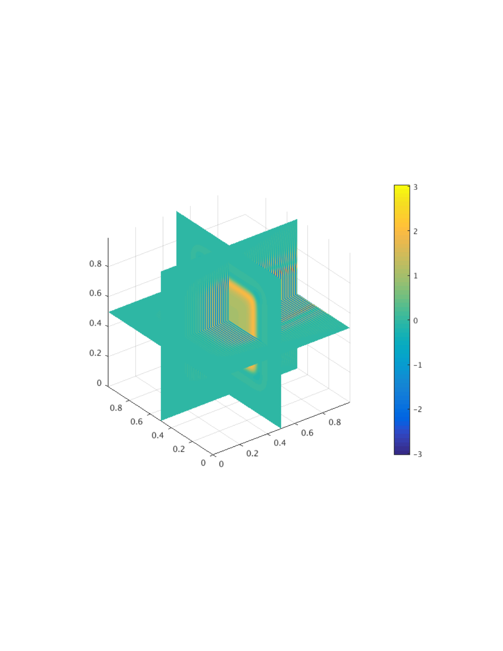
where $I$ is the $3\times 3$ identity matrix and $\omega=408$ . Note that the contrast is approximately 2 and that the magnitude of the oscillation is relatively small: 10% of the magnitude of the bump function $W(x,y,z)$ itself. Nevertheless, to resolve $\epsilon$ at 2 points per wavelength requires at least 200 points in each component direction. We plot the $z$ component of the scattered field $\boldsymbol{E}^{\operatorname{scat}}$ in Figure 1 after solving the integral equation (64).

Refer to caption — Figure 1: The $z$ -component of the electric field, when solving the Maxwell scattering problem (52) with $\omega=408$ , $\mu=I$ and $\epsilon$ defined in (66). The solution is obtained from the representation (65) and the corresponding integral equation (64), discretized with $650^{3}$ points.

Since we do not have an exact solution for this problem, we carry out a numerical convergence study, using a $326\times 326\times 326$ grid followed by a $650\times 650\times 650$ grid, suggesting that six digits of accuracy have been achieved on the coarser grid in both the $L_{2}$ and $L_{\infty}$ norms. The calculation required 61 matrix-vector multiplies and 152 minutes on an Intel Xeon 2.5GHz workstation with 60 cores and 1.5 terabytes of memory.

5.2 Strong isotropic and anisotropic scattering

To study the behavior of our integral equation formulation at higher contrast over a range of frequencies, we consider two additional locally isotropic examples and two anisotropic ones. For the isotropic cases, we let

\epsilon_{222}(x,y,z):=\big(1+W(x,y,z)\big)I,\qquad\epsilon_{444}(x,y,z)=\big(1+3W(x,y,z)\big)I.

Note that $\epsilon_{222}$ has a maximum contrast of 2, while $\epsilon_{444}$ has a maximum contrast of 4. For the anisotropic examples, we let

\epsilon_{234}(x,y,z)=\left(\begin{array}[]{ccc}\epsilon_{1}&0&0\\ 0&\epsilon_{2}&0\\ 0&0&\epsilon_{3}\\ \end{array}\right),\text{ with }\left\{\begin{array}[]{l}\epsilon_{1}(x,y,z)=1+W(x,y,z),\\ \epsilon_{2}(x,y,z)=1+2W(x,y,z),\\ \epsilon_{3}(x,y,z)=1+3W(x,y,z),\end{array}\right.

(67)

and

\epsilon_{dense}(x,y,z)=R_{2}(\phi)R_{1}(\theta)\left(\begin{array}[]{ccc}\epsilon_{1}&0&0\\ 0&\epsilon_{2}&0\\ 0&0&\epsilon_{3}\\ \end{array}\right)R_{1}(\theta)^{\prime}R_{2}(\phi)^{\prime}

(68)

where $\epsilon_{1}$ , $\epsilon_{2}$ , $\epsilon_{3}$ are defined in (67), and the rotation matrices $R_{1}$ and $R_{2}$ are given by

\displaystyle R_{1}(\theta)

\displaystyle=\left(\begin{array}[]{ccc}1&0&0\\ 0&\cos(\theta)&-\sin(\theta)\\ 0&\sin(\theta)&\cos(\theta)\end{array}\right),\quad R_{2}(\phi)

\displaystyle=\left(\begin{array}[]{ccc}\cos(\phi)&-\sin(\phi)&0\\ \sin(\phi)&\cos(\phi)&0\\ 0&0&1\end{array}\right),

(69)

with $\phi(x,y,z)=\pi x$ and $\theta(x,y,z)=\pi y$ .

We first examine the performance of Bi-CGStab, plotting the number of iterations required to achieve a tolerance of $10^{-14}$ as a function of the frequency $\omega$ for both the Helmholtz and Maxwell scattering problems on a $150\times 150\times 150$ grid (Fig. 2). As expected, the number of iterations increases with frequency. Moreover, for a fixed frequency, the number of iterations increases with the contrast. Note, however, that the anisotropy and rotation have only limited impact on the number of iterations. Clearly, while the method is robust at low frequencies, these calculations remain challenging in strong scattering regimes.

Additional details regarding numerical experiments are provided in Tables 1-4. Note that the number of iterations is more or less constant for each fixed problem as the mesh is refined (consistent with the expected behavior of a second kind Fredholm equation). Note also that the number of iterations for the diagonally anisotropic case $\epsilon_{234}$ (Table 2) is about the same as for the case $\epsilon_{dense}$ , where the principal axes have been rotated throughout the domain (Table 3).

In the example $\epsilon_{444}$ , the number of iterations is significantly worse than in any of the other cases, even though it is locally isotropic. Thus, the behavior of the proposed integral equation (64) appears to be controlled by the contrast and frequency more than by anisotropy. The scatterer is approximately $\left(\frac{\omega}{2\pi}\,\sqrt{4}\right)^{3}$ cubic wavelengths in size - on the order of 1000 for the largest value of $\omega$ . Thus, it is not surprising that Bi-CGStab requires many iterations to converge.

Table 1: Summary of numerical results for the locally isotropic permittivity tensor

\epsilon_{222}

. The size is defined to be the number of wavelengths of the incoming field across the unit box supporting the perturbation

\epsilon

, namely

\frac{\omega}{2\pi}

N_{tot}

denotes the total number of unknowns,

n_{side}

denotes the number of points in each linear dimension,

E_{2}

denotes the

L_{2}

error,

E_{\infty}

denotes the

L_{\infty}

error,

N_{matvec}

denotes the number of matrix-vector multiplies required, and

Time

denotes the total time required for the computation in seconds.

Size $\left(\frac{\omega}{2\pi}\right)$	$N_{tot}$	$n_{side}$	$E_{2}$	$E_{\infty}$	$N_{matvec}$	$Time$ $(s)$
$10^{-50}$	$1.03\,10^{6}$	$70$	$1.5\times 10^{-7}$	$1.1\times 10^{-6}$	$22$	$6.4$
$10^{-50}$	$5.18\,10^{6}$	$120$	$1.2\times 10^{-11}$	$7.8\times 10^{-11}$	$22$	$27.7$
$10^{-50}$	$1.75\,10^{7}$	$180$	$1.6\times 10^{-16}$	$1.0\times 10^{-15}$	$22$	$93.6$
$10^{-10}$	$1.03\,10^{6}$	$70$	$1.5\times 10^{-7}$	$1.1\times 10^{-6}$	$22$	$6.6$
$10^{-10}$	$5.18\,10^{6}$	$120$	$1.2\times 10^{-11}$	$7.8\times 10^{-11}$	$22$	$27.5$
$10^{-10}$	$1.75\,10^{7}$	$180$	$1.6\times 10^{-16}$	$1.0\times 10^{-15}$	$22$	$91.9$
$1$	$1.03\,10^{6}$	$70$	$1.5\times 10^{-7}$	$8.2\times 10^{-7}$	$27$	$8.1$
$1$	$5.18\,10^{6}$	$120$	$1.1\times 10^{-11}$	$6.0\times 10^{-11}$	$27$	$33.3$
$1$	$1.75\,10^{7}$	$180$	$2.4\times 10^{-16}$	$8.6\times 10^{-16}$	$27$	$110.1$
$20$	$1.03\,10^{6}$	$70$	$7.3\times 10^{-4}$	$1.1\times 10^{-3}$	$469$	$134.1$
$20$	$5.18\,10^{6}$	$120$	$4.9\times 10^{-10}$	$1.2\times 10^{-9}$	$426$	$487.5$
$20$	$1.75\,10^{7}$	$180$	$1.9\times 10^{-14}$	$1.8\times 10^{-14}$	$426$	$1614.8$

Table 2: Summary of numerical results for the anisotropic permittivity tensor

\epsilon_{234}

. See Table 1 for an explanation of the column headers.

Size $\left(\frac{\omega}{2\pi}\right)$	$N_{tot}$	$n_{side}$	$E_{2}$	$E_{\infty}$	$N_{matvec}$	$Time$ $(s)$
$10^{-50}$	$1.03\,10^{6}$	$70$	$3.1\times 10^{-6}$	$1.9\times 10^{-5}$	$37$	$10.9$
$10^{-50}$	$5.18\,10^{6}$	$120$	$1.7\times 10^{-9}$	$8.5\times 10^{-9}$	$37$	$44.9$
$10^{-50}$	$1.75\,10^{7}$	$180$	$1.7\times 10^{-13}$	$9.9\times 10^{-13}$	$37$	$148.8$
$10^{-10}$	$1.03\,10^{6}$	$70$	$3.1\times 10^{-6}$	$1.9\times 10^{-5}$	$37$	$10.8$
$10^{-10}$	$5.18\,10^{6}$	$120$	$1.7\times 10^{-9}$	$8.5\times 10^{-9}$	$37$	$45.4$
$10^{-10}$	$1.75\,10^{7}$	$180$	$1.7\times 10^{-13}$	$9.9\times 10^{-13}$	$37$	$148.5$
$1$	$1.03\,10^{6}$	$70$	$2.2\times 10^{-6}$	$1.0\times 10^{-5}$	$48$	$14.4$
$1$	$5.18\,10^{6}$	$120$	$1.2\times 10^{-9}$	$4.3\times 10^{-9}$	$48$	$57.2$
$1$	$1.75\,10^{7}$	$180$	$1.2\times 10^{-13}$	$6.4\times 10^{-13}$	$50$	$198.1$
$5$	$1.03\,10^{6}$	$70$	$1.8\times 10^{-6}$	$7.7\times 10^{-6}$	$2125$	$611.8$
$5$	$5.18\,10^{6}$	$120$	$9.6\times 10^{-10}$	$3.0\times 10^{-9}$	$2081$	$2378.1$
$5$	$1.75\,10^{7}$	$180$	$8.9\times 10^{-14}$	$3.6\times 10^{-13}$	$2105$	$7948.1$

Table 3: Summary of numerical results for the anisotropic permittivity tensor

\epsilon_{dense}

. See Table 1 for an explanation of the column headers.

Size $\left(\frac{\omega}{2\pi}\right)$	$N_{tot}$	$n_{side}$	$E_{2}$	$E_{\infty}$	$N_{matvec}$	$Time$ $(s)$
$10^{-50}$	$1.03\,10^{6}$	$70$	$1.3\times 10^{-6}$	$7.7\times 10^{-6}$	$37$	$10.6$
$10^{-50}$	$5.18\,10^{6}$	$120$	$4.1\times 10^{-10}$	$1.8\times 10^{-9}$	$37$	$45.3$
$10^{-50}$	$1.75\,10^{7}$	$180$	$2.0\times 10^{-14}$	$1.6\times 10^{-13}$	$37$	$149.2$
$10^{-10}$	$1.03\,10^{6}$	$70$	$1.3\times 10^{-6}$	$7.7\times 10^{-6}$	$37$	$10.8$
$10^{-10}$	$5.18\,10^{6}$	$120$	$4.1\times 10^{-10}$	$1.8\times 10^{-9}$	$37$	$45.2$
$10^{-10}$	$1.75\,10^{7}$	$180$	$2.0\times 10^{-14}$	$1.6\times 10^{-13}$	$37$	$147.9$
$1$	$1.03\,10^{6}$	$70$	$1.3\times 10^{-6}$	$6.9\times 10^{-6}$	$50$	$14.7$
$1$	$5.18\,10^{6}$	$120$	$4.1\times 10^{-10}$	$2.6\times 10^{-9}$	$51$	$61.0$
$1$	$1.75\,10^{7}$	$180$	$1.9\times 10^{-14}$	$1.1\times 10^{-13}$	$51$	$202.0$
$5$	$1029000$	$70$	$1.7\times 10^{-6}$	$1.1\times 10^{-5}$	$1447$	$412.6$
$5$	$5.18\,10^{6}$	$120$	$5.1\times 10^{-10}$	$2.9\times 10^{-9}$	$1474$	$1697.6$
$5$	$1.75\,10^{7}$	$180$	$1.3\times 10^{-13}$	$2.3\times 10^{-13}$	$1478$	$5687.2$

Table 4: Summary of numerical results for the locally isotropic permittivity tensor

\epsilon_{444}

. See Table 1 for an explanation of the column headers.

Size $\left(\frac{\omega}{2\pi}\right)$	$N_{tot}$	$n_{side}$	$E_{2}$	$E_{\infty}$	$N_{matvec}$	$Time$ $(s)$
$10^{-50}$	$3.75\,10^{5}$	$50$	$8.4\times 10^{-5}$	$4.5\times 10^{-4}$	$37$	$5.0$
$10^{-50}$	$3.00\,10^{6}$	$100$	$3.8\times 10^{-8}$	$2.1\times 10^{-7}$	$38$	$27.9$
$10^{-50}$	$1.01\,10^{7}$	$150$	$1.5\times 10^{-11}$	$9.3\times 10^{-11}$	$38$	$87.7$
$10^{-50}$	$3.19\,10^{7}$	$220$	$8.5\times 10^{-15}$	$1.5\times 10^{-14}$	$38$	$271.9$
$10^{-10}$	$3.75\,10^{5}$	$50$	$8.4\times 10^{-5}$	$4.5\times 10^{-4}$	$37$	$5.1$
$10^{-10}$	$3.00\,10^{6}$	$100$	$3.8\times 10^{-8}$	$2.1\times 10^{-7}$	$38$	$27.9$
$10^{-10}$	$1.01\,10^{7}$	$150$	$1.5\times 10^{-11}$	$9.3\times 10^{-11}$	$38$	$88.7$
$10^{-10}$	$3.19\,10^{7}$	$220$	$8.6\times 10^{-15}$	$1.5\times 10^{-14}$	$38$	$273.9$
$1$	$3.75\,10^{5}$	$50$	$6.9\times 10^{-5}$	$2.5\times 10^{-4}$	$61$	$7.9$
$1$	$3.00\,10^{6}$	$100$	$3.1\times 10^{-8}$	$1.3\times 10^{-7}$	$69$	$49.5$
$1$	$1.01\,10^{7}$	$150$	$1.2\times 10^{-11}$	$4.5\times 10^{-11}$	$72$	$161.5$
$1$	$3.19\,10^{7}$	$220$	$1.6\times 10^{-13}$	$1.7\times 10^{-13}$	$68$	$472.3$
$5$	$3.75\,10^{5}$	$50$	$6.7\times 10^{-5}$	$2.4\times 10^{-4}$	$5774$	$704.0$
$5$	$3.00\,10^{6}$	$100$	$2.9\times 10^{-8}$	$1.3\times 10^{-7}$	$5418$	$3768.8$
$5$	$1.01\,10^{7}$	$150$	$1.2\times 10^{-11}$	$4.4\times 10^{-11}$	$5251$	$11489.8$
$5$	$3.19\,10^{7}$	$220$	$2.3\times 10^{-12}$	$3.1\times 10^{-12}$	$5410$	$36594.8$

6 Discussion

We have presented a collection of Fredholm integral equations for electrostatic, acoustic and electromagnetic scattering problems in anisotropic, inhomogeneous media. In the electrostatic and acoustic cases, our approach appears to be new, and involves recasting the scalar problem of interest in terms of a vector unknown. We have shown that high order accuracy can be achieved using the truncated kernel method of [1] and the FFT. We have also shown that problems with low or moderate contrast are rapidly solved using the Bi-CGStab iterative method, even with nearly one billion unknowns on a single multicore workstation. Once the domain is several wavelengths in size, however, and the contrast is large, we have found that both Bi-CGStab and GMRES perform rather poorly. In our largest high-contrast example, the scatterer is approximately 1000 cubic wavelengths in size, and iterative methods would be expected to require many iterations to converge. This suggests two avenues for further research: either the development of fast, direct solvers (the truncated kernel method of [1] can provide explicit matrix entries) or a preconditioning strategy suitable for this class of problems. We are currently investigating both lines of research and will report our progress at a later date.

References

[1] Felipe Vico, Leslie Greengard, and Miguel Ferrando. Fast convolution with free-space Green’s functions. Journal of Computational Physics, 323:191–203, 2016.
[2] W. C. Chew. Waves and Fields in Inhomogeneous Media. IEEE Press, New York, 1995.
[3] J. D. Jackson. Classical Electrodynamics. John Wiley & Sons: New York, 1975.
[4] L. D. Landau, E. M. Lifshitz, and L. P. Pitaevskii. Electrodynamics of Continuous Media. Pergamon Press, Oxford, 1984.
[5] David L Colton and Rainer Kress. Integral equation methods in scattering theory, volume 57. Wiley, New York, 1983.
[6] Lawrence C. Evans. Partial Differential Equations, volume 19. American Mathematical Society, 2010.
[7] David Gilbarg and Neil S Trudinger. Elliptic partial differential equations of second order. Springer, New York, 2015.
[8] David Lem Colton and Rainer Kress. Inverse acoustic and electromagnetic scattering theory, volume 93. Springer, Berlin, 2013.
[9] Michel Cessenat. Mathematical Methods in Electromagnetism: Linear theory and applications, volume 41. World Scientific, 1996.
[10] P. M. Anselone. Collectively Compact Operator Approximation Theory and Applications to Integral Equations. Prentice Hall, Englewood Cliffs, N.J., 1971.
[11] Roland Potthast et al. Electromagnetic scattering from an orthotropic medium. J. Integral Equations Appl, 11(2):197–215, 1999.
[12] Peter Hähner. On the uniqueness of the shape of a penetrable, anisotropic obstacle. Journal of Computational and Applied Mathematics, 116(1):167–180, 2000.
[13] Lars Hörmander. The Analysis of Linear Partial Differential Operators III, volume 3. Springer-Verlag, 1994.
[14] Carlos E Kenig. Carleman estimates, uniform Sobolev inequalities for second-order differential operators, and unique continuation theorems. In Proceedings of the International Congress of Mathematicians, volume 1, page 2, 1986.
[15] Torsten Carleman. Sur un problème d’unicité pour les systèmes d’équations aux dérivées partielles à deux variables indépendantes. Ark. Mat. Astr. Fys., 26(17):1–9, 1939.
[16] Claus Müller. On the behavior of the solutions of the differential equation $\delta$ u= f (x, u) in the neighborhood of a point. Communications on Pure and Applied Mathematics, 7(3):505–515, 1954.
[17] Andrzej Plis. On non-uniqueness in Cauchy problem for an elliptic second order differential equation. Bull. Acad. Polon. Sci. Sér. Sci. Math. Astronom. Phys, 11:95–100, 1963.
[18] Keith Miller. Nonunique continuation for uniformly parabolic and elliptic equations in self-adjoint divergence form with Hölder continuous coefficients. Archive for Rational Mechanics and Analysis, 54(2):105–117, 1974.
[19] Carlos E Kenig and Nikolai Nadirashvili. A counterexample in unique continuation. Mathematical Research Letters, 7(5/6):625–630, 2000.
[20] Nachman Aronszajn. A unique continuation theorem for solutions of elliptic partial differential equations or inequalities of second order. J. Math. Pures Appl., IX Sér., 36:235–249, 1957.
[21] Herbert Koch and Daniel Tataru. Carleman estimates and unique continuation for second-order elliptic equations with nonsmooth coefficients. Communications on Pure and Applied Mathematics, 54(3):339–360, 2001.
[22] Nachman Aronszajn, Andrzej Krzywicki, and Jacek Szarski. A unique continuation theorem for exterior differential forms on Riemannian manifolds. Arkiv för Matematik, 4(5):417–453, 1962.
[23] Christopher D Sogge. Strong uniqueness theorems for second order elliptic differential equations. American Journal of Mathematics, 112(6):943–984, 1990.
[24] Cédric Bellis and Bojan B Guzina. On the existence and uniqueness of a solution to the interior transmission problem for piecewise-homogeneous solids. Journal of Elasticity, 101(1):29–57, 2010.
[25] R Leis. Exterior boundary-value problems in mathematical physics. Trends in Applications of Pure Mathematics to Mechanics, 11:187–203, 1979.
[26] Mei Song Tong, Zhi-Guo Qian, and Weng Cho Chew. Nyström method solution of volume integral equations for electromagnetic scattering by 3D penetrable objects. IEEE Transactions on Antennas and Propagation, 58(5):1645–1652, 2010.
[27] Pasi Yla-Oijala, Johannes Markkanen, Seppo Jarvenpaa, and Sami P Kiminki. Surface and volume integral equation methods for time-harmonic solutions of Maxwell’s equations. Progress In Electromagnetics Research, 149:15–44, 2014.
[28] Lin E Sun and Weng C Chew. Modeling of anisotropic magnetic objects by volume integral equation methods. Applied Computational Electromagnetics Society Journal, 30(12):1256–1261, 2015.
[29] Matthias M Eller and Masahiro Yamamoto. A Carleman inequality for the stationary anisotropic Maxwell system. Journal de Mathématiques Pures et Appliquées, 86(6):449–462, 2006.
[30] Takashi Okaji. Strong unique continuation property for time harmonic Maxwell equations. Journal of the Mathematical Society of Japan, 54(1):89–122, 2002.
[31] Volker Vogelsang. On the strong unique continuation principle for inequalities of Maxwell type. Mathematische Annalen, 289(1):285–295, 1991.
[32] Roland Potthast. Integral equation methods in electromagnetic scattering from anisotropic media. Mathematical methods in the applied sciences, 23(13):1145–1159, 2000.
[33] Ana Alonso Rodríguez and Mirco Raffetto. Unique solvability for electromagnetic boundary value problems in the presence of partly lossy inhomogeneous anisotropic media and mixed boundary conditions. Mathematical Models and Methods in Applied Sciences, 13(4):597–611, 2003.
[34] Ana Alonso and Alberto Valli. Unique solvability for high-frequency heterogeneous time-harmonic Maxwell equations via the Fredholm alternative theory. Mathematical methods in the applied sciences, 21(6):463–477, 1998.
[35] Christophe Hazard and Marc Lenoir. On the solution of time-harmonic scattering problems for Maxwell’s equations. SIAM Journal on Mathematical Analysis, 27(6):1597–1630, 1996.
[36] H. A. van der Vorst. Bi-CGSTAB: A fast and smoothly converging variant of Bi-CG for the solution of nonsymmetric linear systems. SIAM J. Sci. Stat. Comput., 13:631–644, 1992.