Back and forth from Fock space to Hilbert space: a guide for commuters

Let us start by considering a collection of $N$ identical but distinguishable particles, each of which can be put in one of the $K$ modes of a quantum system, e.g. the $K$ eigenstates of its Hamiltonian. The collective state describing the system is given by

$\displaystyle\left|\Psi\right\rangle=\left|k_{1}\right\rangle\otimes\left|k_{2}\right\rangle\otimes...\otimes\left|k_{N}\right\rangle=\left|k_{1},k_{2},...,k_{N}\right\rangle,$

(1)

or by any linear combination of states of this kind, which all belong to the $K^{N}$-dimensional $N$-particles Hilbert space $\mathscr{H}_{N}=\mathscr{H}_{1}^{\otimes N}$ given by the tensor product of $N$ single-particle spaces $\mathcal{\mathscr{H}}_{1}$, each one with dimension $K$ and basis $\{\left|k_{i}\right\rangle\}_{i}$.

Let us now introduce the notion of indistinguishability [17]. We start by the definition of the permutation operator $\hat{P}_{ij}$, whose effect is to exchange the states of the particles $i$ and $j$ inside any state $\left|\{k_{i}\}_{i}\right\rangle$:

$\displaystyle\hat{P}_{ij}\left|k_{1},k_{2},...,k_{i},...,k_{j},...,k_{N}\right\rangle=\left|k_{1},k_{2},...,k_{j},...,k_{i},...,k_{N}\right\rangle.$

(2)

If the particles are indistinguishable, the overall state of the system $\left|\Psi\right\rangle_{id}$ will be given by linear combination of states (of distinguishable particles) which is invariant under action of $\hat{P}_{ij}$, e.g. states like $\left|\{k_{i}\}_{i}\right\rangle$. It means that $\hat{P}_{ij}\left|\Psi\right\rangle_{id}$ is a state physically indistinguishable from the previous one, i.e. they can differ only for a phase:

$\displaystyle\hat{P}_{ij}\left|\Psi\right\rangle_{id}=e^{\mathrm{i}\phi}\left|\Psi\right\rangle_{id}.$

(3)

Of course, two identical permutations must reproduce the initial state, i.e.:

$\displaystyle\hat{P}_{ij}^{2}\left|\Psi\right\rangle_{id}=e^{2\mathrm{i}\phi}\left|\Psi\right\rangle_{id}=\left|\Psi\right\rangle_{id},$

(4)

and thus the eigenvalues for $\hat{P}_{ij}$ are given by $e^{\mathrm{i}\phi}=\pm 1$.

According to the spin-statistics theorem we have two categories of identical particles: fermions, which are characterized by half-integer spins and anti-symmetric wavefunctions, and bosons, which are characterized by integer spins and symmetric wavefunctions. High precision experiments have confirmed the spin-statistics and established strict probability bounds for a violation to occur [18, 19, 20, 21]. Alternative para-statistics have been suggested earlier in the history of quantum mechanics [22], however we are not discussing here the properties of those kind of particles, e.g. anyons [23].

A state is symmetric or anti-symmetric under the action of $\hat{P}_{ij}$ if, respectively, it maintains or it changes its sign, i.e.:

	$\displaystyle\hat{P}_{ij}\left|\Psi\right\rangle_{F}$	$\displaystyle=-\left|\Psi\right\rangle_{F},$		(5)
	$\displaystyle\hat{P}_{ij}\left|\Psi\right\rangle_{B}$	$\displaystyle=+\left|\Psi\right\rangle_{B}.$		(6)

A symmetric or anti-symmetric state can be built with the proper symmetrization operator $\hat{S}$ or $\hat{A}$, acting on the distinguishable particle state $\left|\Psi\right\rangle$:

	$\displaystyle\hat{S}\left|\Psi\right\rangle$	$\displaystyle=\left|\Psi\right\rangle_{B},$		(7)
	$\displaystyle\hat{A}\left|\Psi\right\rangle$	$\displaystyle=\left|\Psi\right\rangle_{F}.$		(8)

In general, the symmetrization operators can be built as

$\displaystyle\left[\begin{array}[]{c}\hat{S}\\ \hat{A}\end{array}\right]\left|\Psi\right\rangle=\left[\begin{array}[]{c}\left|\Psi\right\rangle_{B}\\ \left|\Psi\right\rangle_{F}\end{array}\right]=\sqrt{\frac{n_{1}!n_{2}!...n_{K}!}{N!}}\sum_{\hat{P}}(\pm 1)^{\sigma(P)}\hat{P}\left|\Psi\right\rangle,$

where we are applying on $\left|\Psi\right\rangle$ all the possible distinct permutations $\hat{P}$ of the $N$ single-particle states $\left|k_{i}\right\rangle$ included in $\left|\Psi\right\rangle$, each one multiplied by the sign of the permutation $(-1)^{\sigma(P)}$, where $\sigma(P)$ is the number of particle exchanges occurred in the permutation $\hat{P}$, when we are dealing with fermions. Notice that any $N$-particle permutation $\hat{P}$ can be built by composing a proper sequence of two-particle permutations $\hat{P}_{ij}$, and the same is true for the operators $\hat{A}$ and $\hat{S}$. The states should be then properly normalized with the prefactor under square root, where $n_{k}$ indicates the number of particles occupying the state $k$, i.e., the number of times that $k$ occurs in $\left|\Psi\right\rangle$.

¿From the anti-symmetrization procedure for fermions, we derive the Pauli exclusion principle, that forbids two fermions to occupy the same state: indeed, if this was the case, e.g. for the particles $i$ and $j$, we would have contemporarily

	$\displaystyle\hat{P}_{ij}\left|\Psi\right\rangle_{F}$	$\displaystyle=-\left|\Psi\right\rangle_{F},$		(13)
	$\displaystyle\hat{P}_{ij}\left|\Psi\right\rangle_{F}$	$\displaystyle=\left|\Psi\right\rangle_{F},$		(14)

where the first equality comes from Eq. (5), while the second one comes from the fact that the two particles occupy the same state. The only possible conclusion is that our state is the null vector.

In order to properly describe states and operators taking into account the indistinguishability of particles we should move to the formalism of second quantization [24], where states belong to the bosonic or fermionic Fock space $\mathscr{F}$, that is a space containing states with a number of particles that in principle is not fixed. The number states (basis states) of the Fock space can be represented as

$\displaystyle\left|n_{1},n_{2},...,n_{K}\right\rangle_{B(F)},$

(15)

with the fundamental constraint $n_{i}\in\{0,1\}$ holding only for fermions, because of Pauli’s principle. If we deal with a fixed number $N$ of particles, there is the additional constraint $\sum_{i=1}^{K}n_{i}=N$. In this last case, we are operating in the subspace of $\mathscr{F}$ called $\mathscr{F}_{N}$. Indeed the Fock space is given by:

$\displaystyle\mathscr{F}=\bigoplus_{N=0}^{\infty}\mathscr{F}_{N}.$

(16)

These number states coincide with the states of Eq. (1) except for the relabeling (and the symmetrization). Indeed, while in the first quantization formalism we specify for each particle $i$ ($i=1,...,N$) the state/mode $k_{i}$ that it occupies, in the second quantization formalism we treat particles as excitation of the modes of a field, therefore for each mode $i$ ($i=1,...,K$) we specify how many excitation/particles $n_{i}$ it contains, since we cannot distinguish among them (see Fig. 1).

The total number of particles $N$ can be changed through the application of creation and annihilation (or destruction) operators, respectively denoted as $\hat{a}_{i}^{\dagger}$ and $\hat{a}_{i}$. These operators create or destroy a particle in the mode/state $i$, so they connect the Fock subspaces with a different number of particles:

	$\displaystyle\hat{a}_{i}^{\dagger}$	$\displaystyle:\mathscr{F}_{N}\rightarrow\mathscr{F}_{N+1},$		(17)
	$\displaystyle\hat{a}_{i}$	$\displaystyle:\mathscr{F}_{N}\rightarrow\mathscr{F}_{N-1}.$		(18)

In more detail, these operators are defined by the following commutation rules:

	$\displaystyle\left[\hat{a}_{i},\hat{a}_{j}\right]_{\mp}$	$\displaystyle=\left[\hat{a}_{i}^{\dagger},\hat{a}_{j}^{\dagger}\right]_{\mp}=0,$		(19)
	$\displaystyle\left[\hat{a}_{i},\hat{a}_{j}^{\dagger}\right]_{\mp}$	$\displaystyle=\delta_{i,j},$		(20)

where the upper sign, denoting the commutator, holds for bosons, while the lower sign, denoting the anti-commutator, holds for fermions. It is quite important to stress, therefore, that fermionic creation (annihilation) operators do anticommute: therefore, when we exchange their order, we have to add a minus sign for each permutation we perform.

Upon denoting by $\left|0\right\rangle$ the vacuum state, corresponding to a state with no particle, i.e. $\left|0,0,...,0\right\rangle$ (not to be confused with the null vector), we can build any number state as

$\displaystyle\left|n_{1},n_{2},...,n_{K}\right\rangle_{B(F)}=\prod_{i=1}^{K}\frac{1}{\sqrt{n_{i}!}}\left(\hat{a}_{i}^{\dagger}\right)^{n_{i}}\left|0\right\rangle.$

(21)

From the commutation rules, we also deduce the action of the creation and annihilation operators on the number states:

	$\displaystyle\hat{a}_{i}^{\dagger}\left|n_{1},n_{2},...,n_{i},...,n_{K}\right\rangle_{B(F)}$	$\displaystyle=\begin{cases}\sqrt{n_{i}+1}\left|n_{1},n_{2},...,n_{i}+1,...,n_{K}\right\rangle_{B}\\ (1-n_{i})(-1)^{\sigma_{i}}\left|n_{1},n_{2},...,1-n_{i},...,n_{K}\right\rangle_{F}\,,\end{cases}$		(22)
	$\displaystyle\hat{a}_{i}\left|n_{1},n_{2},...,n_{i},...,n_{K}\right\rangle_{B(F)}$	$\displaystyle=\begin{cases}\sqrt{n_{i}}\left|n_{1},n_{2},...,n_{i}-1,...,n_{K}\right\rangle_{B}\\ n_{i}(-1)^{\sigma_{i}}\left|n_{1},n_{2},...,1-n_{i},...,n_{K}\right\rangle_{F}\,,\end{cases}$		(23)

where the $\sigma_{i}$ exponent is due to the anti-commuting rules and is given by

$\displaystyle\sigma_{i}=\sum_{k=1}^{i-1}n_{k}.$

(24)

From Eqs. (22)-(23) we straightforwardly deduce that

	$\displaystyle\hat{a}_{i}\left|n_{1},n_{2},...,n_{i},...,n_{K}\right\rangle$	$\displaystyle=0\quad\mathrm{if}\,n_{i}=0,$		(25)
	$\displaystyle\hat{a}_{i}^{\dagger}\hat{a}_{i}\left|n_{1},n_{2},...,n_{i},...,n_{K}\right\rangle$	$\displaystyle=n_{i}\left|n_{1},n_{2},...,n_{i},...,n_{K}\right\rangle.$		(26)

The last equation gives the definition of the number operator

$\displaystyle\hat{n}_{i}=\hat{a}_{i}^{\dagger}\hat{a}_{i},$

(27)

that counts the number of particles in the mode $i$.

Let us now consider a single-particle operator $\hat{O}_{j}$ acting on the particle $j$. It is apparent that we must have

$\displaystyle\hat{P}_{ij}\hat{O}_{j}\hat{P}_{ij}=\hat{O_{i}}.$

(28)

Then, for a many-particle operator $\hat{O}$, we will say that this operator is invariant under particle exchange (permutation symmetry) if, for any couple of particles $i$ and $j$, the following relation holds:

$\displaystyle\hat{P}_{ij}\hat{O}\hat{P}_{ij}=\hat{O}.$

(29)

However, the previous property does not mean that the operator $\hat{O}$ must be invariant also under the action of $\hat{A}$ and $\hat{S}$, but it implies that these symmetry operators must commute with $\hat{O}$. It means, therefore, that for $\hat{O}=\hat{H}$ the evolution preserves the symmetry of bosonic and fermionic states, i.e. their subspaces

$$\mathscr{F}_{N}^{B}=\hat{S}\mathscr{H}_{N}$$

(30)

and

$$\mathscr{F}_{N}^{F}=\hat{A}\mathscr{H}_{N}$$

(31)

are not mixed, since the Hamiltonian $\hat{H}$ and $\hat{S}\,(\hat{A})$ have a common set of orthogonal eigenstates. Therefore, this kind of operators can be used in the second quantization formalism with identical particle states in the same way they were used in first quantization, because they preserve the permutation symmetry. We remind here that second quantization representation is strictly connected with the choice of the basis $\{\left|a_{i}\right\rangle\}_{i}$ in which the operators $\hat{a}_{i}^{\dagger}\,(\hat{a}_{i})$ are creating (destroying) particles: indeed, if $\hat{a}_{i}^{\dagger}\,(\hat{a}_{i})$ creates (destroys) a particle in the i-th eigenstate of the Hamiltonian, we can define a change of basis and build a new set of operators $\hat{b}_{i}^{\dagger}\,(\hat{b}_{i})$ that create (destroy) particles in the i-th eigenstate of any other operator $\hat{O}$ (e.g. in the i-th site of a lattice for the position operator):

$\displaystyle\left|b_{i}\right\rangle=\left[\hat{b}_{i}^{\dagger}\right]\left|0\right\rangle=\sum_{j}\left\langle a_{j}\middle|b_{i}\right\rangle\left|a_{j}\right\rangle=\left[\sum_{j}\left\langle a_{j}\middle|b_{i}\right\rangle\hat{a}_{j}^{\dagger}\right]\left|0\right\rangle.$

(32)

Here and in the rest of the article we apply the tools introduced in the previous section to the specific case of $N=2$ identical particles. Despite the small number of particles, this example shows most of the peculiarities related to indistinguishability, and illustrates how to deal with both Fock and Hilbert descriptions to conveniently describe the physics of the system.

In the Hilbert space $\mathscr{H}_{2}$ (for distinguishable particles), the basis set is given by $\{\left|i,j\right\rangle\}_{i,j}$. According to the symmetrization procedures described above for a 2-boson state we have

$\displaystyle\left|i,j\right\rangle_{s}=\begin{cases}\frac{1}{\sqrt{2}}\left(\left|i,j\right\rangle+\left|j,i\right\rangle\right)&\mathrm{for}\,i<j\\ \left|i,i\right\rangle&\mathrm{for}\,i=j\,,\end{cases}$

(33)

while for a 2-fermion state the allowed basis set is given by:

$\displaystyle\left|i,j\right\rangle_{a}=\frac{1}{\sqrt{2}}\left(\left|i,j\right\rangle-\left|j,i\right\rangle\right)\quad\mathrm{for}\,i<j,$

(34)

where the constraint $j>i$ avoids overcounting in the basis set, since

	$\displaystyle\left|j,i\right\rangle_{s}$	$\displaystyle=\left|i,j\right\rangle_{s},$		(35)
	$\displaystyle\left|j,i\right\rangle_{a}$	$\displaystyle=-\left|i,j\right\rangle_{a}.$		(36)

It is easy to check that these two new basis sets are orthogonal and related to the previous one by

$\displaystyle\{\left|i,j\right\rangle\}_{i,j}=\{\left|i,j\right\rangle_{s}\}_{i,j}\cup\{\left|i,j\right\rangle_{a}\}_{i,j}.$

(37)

Indeed, the dimension $d_{B}$ of the basis set for bosonic particles is given by

$\displaystyle d_{B}=K+\frac{K(K-1)}{2}=\frac{K(K+1)}{2},$

(38)

while the dimension $d_{F}$ of the fermionic basis set is given by

$\displaystyle d_{F}=\frac{K(K-1)}{2},$

(39)

and

$\displaystyle d_{B}+d_{F}=K^{2}=\dim(\mathscr{H}_{2}).$

(40)

Overall, the Hilbert space $\mathscr{H}_{2}$ is decomposed into two subspaces [25]: one contains only symmetric states, while the other one only anti-symmetric states, see Fig. 2. These subspaces are, in turn, the 2-particle restrictions of the Fock spaces for bosons and fermions, namely $\mathscr{F}_{2}^{B}$ and $\mathscr{F}_{2}^{F}$:

$\displaystyle\mathscr{H}_{2}=\mathscr{F}_{2}^{B}\oplus\mathscr{F}_{2}^{F}.$

(41)

Each subspace is obtained, in general, by applying the proper symmetry operators over $\mathscr{H}_{2}$:

	$\displaystyle\mathscr{F}_{2}^{B}$	$\displaystyle=\hat{S}\mathscr{H}_{2},$		(42)
	$\displaystyle\mathscr{F}_{2}^{F}$	$\displaystyle=\hat{A}\mathscr{H}_{2},$		(43)

which are given by the following projectors:

	$\displaystyle\hat{S}$	$\displaystyle=\sum_{i}\left|i,i\right\rangle\left\langle i,i\right|+\sum_{i,j>i}\frac{1}{2}\left(\left|i,j\right\rangle+\left|j,i\right\rangle\right)\left(\left\langle i,j\right|+\left\langle j,i\right|\right),$		(44)
	$\displaystyle\hat{A}$	$\displaystyle=\sum_{i,j>i}\frac{1}{2}\left(\left|i,j\right\rangle-\left|j,i\right\rangle\right)\left(\left\langle i,j\right|-\left\langle j,i\right|\right).$		(45)

However, the action of $\hat{S}$ and $\hat{A}$ is not enough to write operators (or states) in the Fock space. Indeed, if we consider the bosonic operator $\hat{O}_{B}=\hat{S}\hat{O}\hat{S}$, in order to properly represent it in the Fock space we still have to perform a change of basis. Therefore, sometimes it could be useful to perform both operations in a single step, by writing the symmetry operators in a mixed-basis representation (where the bras are states of $\mathscr{H}_{2}$, while kets are states of $\mathscr{F}_{2}$):

	$\displaystyle\hat{S}$	$\displaystyle=\sum_{i}\left|i,i\right\rangle_{s}\left\langle i,i\right|+\sum_{i,j>i}\left|i,j\right\rangle_{s}\frac{1}{\sqrt{2}}\left(\left\langle i,j\right|+\left\langle j,i\right|\right),$		(46)
	$\displaystyle\hat{A}$	$\displaystyle=\sum_{i,j>i}\left|i,j\right\rangle_{a}\frac{1}{\sqrt{2}}\left(\left\langle i,j\right|-\left\langle j,i\right|\right).$		(47)

so that we can write the operator $\hat{O}_{B}$ in $\mathscr{F}_{2}$ directly as $\hat{S}\hat{O}\hat{S}^{\dagger}$ (a similar discussion also holds for fermionic operators).

Even if in general this is not true, we observe that for the case $N=2$ we have

$\displaystyle\hat{S}+\hat{A}=\hat{I},$

(48)

in agreement with Eq. (37). In conclusion, a distinguishable-particle operator $\hat{O}$ in $\mathscr{H}_{2}$ is invariant under particle-exchange symmetry if and only if the following decomposition holds:

$\displaystyle\hat{O}=\hat{S}\hat{O}\hat{S}+\hat{A}\hat{O}\hat{A}=\hat{O}_{s}+\hat{O}_{a},$

(49)

i.e. the operator is the sum of its projections over the bosonic and fermionic subspaces of $\mathscr{H}_{2}$. This means that $\hat{O}$ does not mix states belonging to subspaces with different symmetries (i.e., fermionic and bosonic), and it commutes with $\hat{A}$ and $\hat{S}$. If this property holds also for the Hamiltonian $\hat{H}$, it is possible to perform a symmetrization only over the state vectors without modifying the operators. Indeed, $\hat{S}$ and $\hat{A}$ are projectors, $\hat{S}=\hat{S}^{\dagger}$ and $\hat{S}^{n}=\hat{S}$, and are orthogonal, i.e. $\hat{S}\hat{A}=\hat{A}\hat{S}=0$. The dynamics thus conserves symmetries, and this is sufficient to get the right expectation values:

$$\hat{H}_{s}=\hat{S}\hat{H}\hat{S}=\hat{H}\hat{S}^{2}=\hat{H}\hat{S},$$

(50)

$$\hat{H}_{s}\left|\Psi\right\rangle_{s}=\hat{H}\hat{S}^{2}\left|\Psi\right\rangle=\hat{H}\left|\Psi\right\rangle_{s},$$

(51)

$$O_{s}={}_{s}\langle\Psi|\hat{O}_{s}|\Psi\rangle_{s}=\left\langle\Psi\right|\hat{S}^{2}\hat{O}\hat{S}^{2}\left|\Psi\right\rangle=\left\langle\Psi\right|\hat{S}\hat{O}\hat{S}\left|\Psi\right\rangle={}_{s}\langle\Psi|\hat{O}|\Psi\rangle_{s}.$$

(52)

Clearly for the 2-particle case, the evaluation of expectation values and dynamics of the system can be conveniently obtained in the Hilbert space, starting with a properly (anti-)symmetrized state[26], namely $\left|\Psi\right\rangle_{(a)s}$. Then, with a proper reshaping operation, observables may be recast in the Fock space, see Fig. 3. This procedure presents advantages compared to a direct calculation in the Fock space where each particle loses its identity. For instance, the operation of partial trace over the degrees of freedom of one particle is straightforward in the Hilbert space, while it is more delicate in the Fock space, where the natural basis set is the occupation number. Moreover, the indexing of the basis in the Fock space is not trivial to handle [27], and a convenient way to rank the basis vectors should be considered in the numerical implementation (see Section 5). Therefore, it is often the case that the dynamics and all the required observables are evaluated in the Hilbert space, after a proper symmetrization of the initial state.

Given the basis sets for the symmetric and antisymmetric subspaces, $\{\left|i,j\right\rangle_{s}\}_{i,j\geq i}$ and $\{\left|i,j\right\rangle_{a}\}_{i,j>i}$, their union $\mathcal{B}^{*}=\{\left|i,j\right\rangle_{s}\}_{i,j\geq i}\cup\{\left|i,j\right\rangle_{a}\}_{i,j>i}$ is a basis set for the whole Hilbert space $\mathscr{H}_{2}$. As discussed in the previous section, we typically use the distinguishable-particle basis set, hereafter labeled $\mathcal{B}=\{\left|i,j\right\rangle\}_{i,j}$.

The bosonic operator $\hat{O}_{B}$ may be represented with a $d_{B}\times d_{B}$ matrix defined on $\mathscr{F}_{2}^{B}$, but also with a $K^{2}\times K^{2}$ matrix acting on $\mathscr{H}_{2}$. Adding $d_{F}$ rows and $d_{F}$ columns full of zeros, we may extend the Fock matrix $\hat{O}_{B}^{\mathscr{F}}$: the first $d_{B}$ rows and columns involve only bosonic states, while the additional lines only the fermionic states (none, since it is a bosonic operator):

$\displaystyle\hat{O}_{B}^{\mathscr{H}}|_{\mathcal{B}^{*}}=\left(\begin{array}[]{ccc|c}&&&\\ &\text{\huge{$\hat{O}_{B}^{\mathscr{F}}$}}&&\text{\huge{$0$}}\\ &&&\\ \hline\cr&&&\\ &\text{\huge{$0$}}&&\text{\huge{$0$}}\end{array}\right).$

When the basis set is given by $\mathcal{B}^{*}$, whose symmetric part coincides with the basis of $\mathcal{\mathscr{F}}_{2}^{B}$, the representation $\hat{O}_{B}^{\mathcal{\mathscr{H}}}|_{\mathcal{B}^{*}}$ is valid in $\mathscr{H}_{2}$. In order to represent operators in the basis $\mathcal{B}$ of distinguishable particles, we need to reverse this transformation, that is:

$\displaystyle\hat{O}_{B}^{\mathcal{\mathscr{H}}}|_{\mathcal{B}}=\hat{S}^{\dagger}\hat{O}_{B}^{\mathcal{\mathscr{H}}}|_{\mathcal{B}^{*}}\hat{S}.$

(58)

The relation between the elements of a bosonic operator in the Fock (basis $\mathcal{B}_{s}^{*}=\{\left|i,j\right\rangle_{s}\}_{i,j\geq i}$) and in the Hilbert space (basis $\mathcal{B}=\{\left|i,j\right\rangle\}_{i,j}$) is the following:

$\displaystyle\left(O_{B}^{\mathcal{\mathscr{H}}}\right)_{i,j;k,l}$

$\displaystyle=\left\langle i,j\right|\hat{O}_{B}^{\mathcal{\mathscr{H}}}|_{\mathcal{B}}\left|k,l\right\rangle=\frac{1}{2}\left(O_{B}^{\mathscr{F}}\right)_{i,j;k,l}\left(1+\epsilon\delta_{i,j}\right)\left(1+\epsilon\delta_{k,l}\right),$

(59)

where $\epsilon=\sqrt{2}-1$.

Analogous arguments apply to the fermionic case, thus

$\displaystyle\hat{O}_{F}^{\mathscr{H}}|_{\mathcal{B}}=\hat{A}^{\dagger}\hat{O}_{F}^{\mathscr{H}}|_{\mathcal{B}^{*}}\hat{A},$

(60)

where

$\displaystyle\hat{O}_{F}^{\mathscr{H}}|_{\mathcal{B}^{*}}=\left(\begin{array}[]{c|ccc}\text{\huge{$0$}}&&\text{\huge{$0$}}&\\ \hline\cr\\ \text{\huge{$0$}}&&\text{\huge{$\hat{O}_{F}^{\mathscr{F}}$}}\\ \\ \end{array}\right).$

Again, the transformation of a fermionic operator in the Fock space (basis $\mathcal{B}_{a}^{*}=\{\left|i,j\right\rangle_{a}\}_{i,j>i}$) to the Hilbert space (basis $\mathcal{B}=\{\left|i,j\right\rangle\}_{i,j}$) is given by

$\displaystyle\left(O_{F}^{\mathscr{H}}\right)_{i,j;k,l}=\frac{1}{2}\left(O_{F}^{\mathscr{F}}\right)_{i,j;k,l}\left(1-\delta_{i,j}\right)\left(1-\delta_{k,l}\right)\varsigma_{i,j}\varsigma_{k,l},$

(65)

where $\varsigma_{i,j}=\mathrm{sgn}(j-i)$.

In the case of a 2-particle bosonic (fermionic) operator, the transformation laws from Fock to Hilbert space of distinguishable particles are thus given by equations (59) and (65), respectively. However, one should remind that the Fock space elements exist only for $i\leq j$ ($i<j$ for fermions), so indices in $\left(O_{F}^{\mathscr{F}}\right)_{i,j;k,l}$ must be exchanged if $i>j$ and/or $k>l$. Moreover, if $i=j$ or $k=l$, the corresponding elements are zero.

Notice that if the dynamics is evaluated in the Hilbert space, the reshaping operation needed to recast observables in the Fock space is given by the inverse equations of (59) and (65).

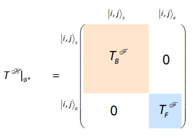
Let us consider a native Hilbert operator $\hat{T}^{\mathscr{H}}$, i.e. an operator which arises naturally in the distinguishable particles Hilbert space $\mathscr{H}_{2}$ where the basis set is given by $\mathcal{B}$. Such an operator conserves parity, being invariant under particle exchange, thus it does not mix states with different symmetries; therefore it is equivalent to the sum of its projections with defined symmetries: $\hat{T}^{\mathscr{H}}=\hat{S}\hat{T}^{\mathscr{H}}\hat{S}^{\dagger}+\hat{A}\hat{T}^{\mathscr{H}}\hat{A}^{\dagger}$, see Fig. 4. Overall, we have that $\mathscr{H}_{2}^{s}$ and $\mathscr{H}_{2}^{a}$ are invariant subspaces for $\hat{T}^{\mathscr{H}}$.

Since the operator acts on states of distinguishable particles, it contains both bosonic and fermionic components, which can be isolated with a suitable transformation. An interesting example is the kinetic term $\hat{T}$ in the Hubbard model, which can be derived from the discretization of the laplacian terms in the Schrödinger equation, and describes the hopping of the two particles along a chain with $K$ sites. In the distinguishable particles framework we have

$\displaystyle\hat{T}^{\mathscr{H}}=\left[-J\sum_{i=1}^{K}(\left|i\right\rangle\left\langle i+1\right|+\left|i+1\right\rangle\left\langle i\right|)\right]\otimes I_{1}+I_{1}\otimes\left[-J\sum_{i=1}^{K}(\left|i\right\rangle\left\langle i+1\right|+\left|i+1\right\rangle\left\langle i\right|)\right],$

(66)

where $I_{1}=\sum_{i=1}^{K}\left|i\right\rangle\left\langle i\right|$ is the single-particle identity operator, and $J$ is a scale factor that represents the tunneling amplitude between adjacent sites and depends on physical parameters of the system, such as the particle mass and the distance between the discrete sites. The form of $\hat{T}$ for identical particles in the Fock space is

$\displaystyle\hat{T}^{\mathscr{F}}=-J\sum_{i=1}^{K}(\hat{c}_{i}^{\dagger}\hat{c}_{i+1}+\hat{c}_{i+1}^{\dagger}\hat{c}_{i}),$

(67)

where $\hat{c}_{i}$ is an annihilation operator (for bosons or fermions) and $\hat{c}_{i}^{\dagger}$ the corresponding creation operator for the mode $i$. Given the results of the previous section, we conclude that the representation of the bosonic/fermionic operator in the Fock space can be obtained from $\hat{T}^{\mathscr{H}}$ by a simple change of basis, followed by a projection over the subspace with the required symmetry. Considering $\hat{T}$ a bosonic operator, we have

$\displaystyle\hat{T}^{\mathscr{F}}_{B}=\hat{S}\hat{T}^{\mathscr{H}}\hat{S}^{\dagger}.$

(68)

Let us check the previous results in some significant cases:

	$\displaystyle{}_{s}\langle k,k+1|\hat{T}^{\mathscr{F}}_{B}|k,k\rangle_{s}$	$\displaystyle=-J{}_{s}\langle k,k+1|\hat{c}_{k+1}^{\dagger}\hat{c}_{k}|k,k\rangle_{s}=-\sqrt{2}J,$		(69)
	$\displaystyle{}_{s}\langle k,k+1|\hat{S}\hat{T}^{\mathscr{H}}\hat{S}^{\dagger}|k,k\rangle_{s}$	$\displaystyle=\frac{1}{\sqrt{2}}\left(\left\langle k,k+1\right|+\left\langle k+1,k\right|\right)\hat{T}^{\mathscr{H}}\left|k,k\right\rangle=-\sqrt{2}J,$		(70)
	${}_{s}\langle k,l+1|\hat{T}^{\mathscr{F}}_{B}|k,l\rangle_{s}$	$\displaystyle\underset{{}_{l\neq k,k-1}}{=}-J{}_{s}\langle k,l+1|\hat{c}_{l+1}^{\dagger}\hat{c}_{l}|k,l\rangle_{s}=-J,$		(71)
	${}_{s}\langle k,l+1|\hat{S}\hat{T}^{\mathscr{H}}\hat{S}^{\dagger}|k,l\rangle_{s}$	$\displaystyle\underset{{}_{l\neq k,k-1}}{=}\frac{1}{\sqrt{2}}\left(\left\langle k,l+1\right|+\left\langle l+1,k\right|\right)\hat{T}^{\mathscr{H}}\frac{1}{\sqrt{2}}\left(\left|k,l\right\rangle+\left|l,k\right\rangle\right)$
		$\displaystyle\quad=-J.$		(72)

Analogous results may be obtained for fermions, where additional attention to the anticommutation relation is required to handle periodic boundary conditions (PBC). If a state like $\left|k,K\right\rangle_{a}$ is connected to a state like $\left|1,k\right\rangle_{a}$, e.g. $K$ jumps over the border, we should account for an additional minus sign due to the reordering of the anti-commuting fermionic operators. Indeed (we denote the state with no particle with $\left|0\right\rangle$):

	$\displaystyle\left|1,k\right\rangle_{a}$	$\displaystyle=\hat{c}_{1}^{\dagger}\hat{c}_{k}^{\dagger}\left|0\right\rangle,$		(73)
	$\displaystyle\hat{c}_{K+1}^{\dagger}\hat{c}_{K}\left|k,K\right\rangle_{a}$	$\displaystyle\underset{{}_{PBC}}{=}\hat{c}_{1}^{\dagger}\hat{c}_{K}\left|k,K\right\rangle_{a}=\hat{c}_{1}^{\dagger}\hat{c}_{K}\hat{c}_{k}^{\dagger}\hat{c}_{K}^{\dagger}\left|0\right\rangle$
		$\displaystyle=-\hat{c}_{1}^{\dagger}\hat{c}_{k}^{\dagger}\hat{c}_{K}\hat{c}_{K}^{\dagger}\left|0\right\rangle=-\hat{c}_{1}^{\dagger}\hat{c}_{k}^{\dagger}\left|0\right\rangle=-\left|1,k\right\rangle_{a}.$		(74)

The same results may be obtained without any change of basis, that is by simply applying the operator $\hat{T}^{\mathscr{H}}$ only over the proper (anti-)symmetrized states (this is equivalent to applying the transformation described by $\hat{S}$ or $\hat{A}$). However, the spectrum of the operator $\hat{S}\hat{T}^{\mathscr{H}}\hat{S}^{\dagger}$ is substantially the spectrum of the bosonic operator, while the spectrum of $\hat{T}^{\mathscr{H}}$ contains also the fermionic eigenvalues of $\hat{A}\hat{T}^{\mathscr{H}}\hat{A}^{\dagger}$.

Further, we observe that the representation of $\hat{T}^{\mathscr{F}}_{B}$ in the basis $\mathcal{B}$ of $\mathscr{H}_{2}$ is quite interesting. Indeed, it contains terms like $-J|i+1,j\rangle_{s}{}_{s}\langle i,j|$, which can be rewritten as:

	$\displaystyle-J$	$\displaystyle|i+1,j\rangle_{s}{}_{s}\langle i,j|=$		(75)
		$\displaystyle=-\frac{J}{2}\left(\left|i+1,j\right\rangle\left\langle i,j\right|+\left|j,i+1\right\rangle\left\langle j,i\right|+\left|j,i+1\right\rangle\left\langle i,j\right|+\left|i+1,j\right\rangle\left\langle j,i\right|\right).$

This suggests that the Fock operator not only produces transitions where one particle hops from a site to a nearest-neighbour one, but can also allows the two particles to exchange their position: the third term in brackets in the RHS of the previous equation sees the second particle in position $i$ jumping on the site $i+1$, and then exchanging its position with the first particle, previously located on site $j$. These exchange terms are a consequence of the fact that when we rewrite the operator in the Hilbert space of distinguishable particles, it must bear signs of the exchange symmetry, due to the fact that it is actually acting on identical particles (in this case, bosons). The original operator $\hat{T}^{\mathscr{H}}$ does not contain these terms, but they appear when we apply the transformation $\hat{S}\hat{T}^{\mathscr{H}}\hat{S}^{\dagger}$.

Let us now consider our quantum system of $N=2$ identical particles, whose evolution is ruled by the Hamiltonian $\hat{H}^{\mathscr{F}}$. Their dynamics can be directly calculated in the Hilbert space of distinguishable particles $\mathscr{H}_{2}$: we can properly (anti-)symmetrize the initial state and get the final state of the evolution with the required symmetry, exactly as we had carried over the evolution in the Fock space. This can be done either using the Fock Hamiltonian $\hat{H}^{\mathscr{F}}$ rewritten in the Hilbert space (see Eqs. (59) and (65)), or using directly the equivalent Hamiltonian $\hat{H}^{\mathscr{H}}$ for distinguishable particles, provided that it conserves parity (i.e., it is invariant under particle exchange). Indeed, projecting $\hat{H}^{\mathscr{H}}$ over the subspaces with the proper symmetry (i.e., using $\hat{S}$ or $\hat{A}$) - and/or applying it only over properly symmetrized states - is equivalent to using $\hat{H}^{\mathscr{F}}$, as we have just seen in the previous section.

In order to simplify the notation, let us define a factor $g$ to distinguish between bosons ($g=+1$) and fermions ($g=-1$). If needed, we will use the subscript $\left|...\right\rangle_{g}$ to denote symmetrized or anti-symmetrized states.

The density operator is the fundamental quantity for evaluating the expectation values of all the observables characterizing the system. The density operator can be calculated in the Hilbert space as usual:

$\displaystyle\rho^{\mathscr{H}}(t)=\left|\Psi(t)\right\rangle\left\langle\Psi(t)\right|,$

(76)

and then recast in the Fock space using Eq. (59) for bosons ($j\geq i$, $l\geq k$):

$\displaystyle\rho_{i,j;k,l}^{\mathscr{F}}=\frac{2}{\left(1+\epsilon\delta_{i,j}\right)\left(1+\epsilon\delta_{k,l}\right)}\rho_{i,j;k,l}^{\mathscr{H}},$

(77)

and Eq. (65) for fermions ($j>i$, $l>k$):

$\displaystyle\rho_{i,j;k,l}^{\mathscr{F}}=2\rho_{i,j;k,l}^{\mathscr{H}},$

(78)

where, within the index constraint, we have $\varsigma_{i,j}=\varsigma_{k,l}=1$. Notice that if $\left|\Psi(t)\right\rangle=\sum_{i,j}\beta_{i,j}(t)\left|i,j\right\rangle$, we should remember that for exchange symmetry

$\displaystyle\beta_{i,j}(t)=g\cdot\beta_{j,i}(t),$

(79)

and then we have

$\displaystyle\rho^{\mathscr{H}}(t)=\sum_{i,j}\sum_{k,l}\beta_{i,j}(t)\beta_{k,l}^{*}(t)\left|i,j\right\rangle\left\langle k,l\right|.$

(80)

If in the Fock space we have

$\displaystyle\rho^{\mathscr{F}}(t)=\sum_{i,j\geq i}\sum_{k,l\geq k}\alpha_{i,j}(t)\alpha_{k,l}^{*}(t)|i,j\rangle_{g}{}_{g}\langle k,l|,$

(81)

it is easy to show that the proper (anti-)symmetrization of the Hilbert matrix elements

$\displaystyle\alpha_{i,j}(t)=\begin{cases}\dfrac{\beta_{i,j}(t)+g\cdot\beta_{j,i}(t)}{\sqrt{2}}=\sqrt{2}\beta_{i,j}(t)&\forall\,i<j\\[10.00002pt] \beta_{i,i}(t)\dfrac{(1+g)}{2}&\forall\,i=j\end{cases}$

(82)

gives exactly the expected results in the Fock space (see Eqs. (77) and (78)).

The expectation value of the number operator $\hat{n}_{k}$, corresponding to the average number of particles in the mode $k$, can be calculated as follows:

	$\displaystyle\left\langle n_{k}\right\rangle$	$\displaystyle=\mathrm{Tr}[\rho^{\mathscr{F}}(t)\hat{n}_{k}]=\mathrm{Tr}[\rho^{\mathscr{F}}(t)\hat{c}_{k}^{\dagger}\hat{c}_{k}]$
		$\displaystyle=\sum_{i}{}_{g}\langle i,i|\rho^{\mathscr{F}}(t)\hat{c}_{k}^{\dagger}\hat{c}_{k}|i,i\rangle_{g}+\sum_{i,j>i}{}_{g}\langle i,j|\rho^{\mathscr{F}}(t)\hat{c}_{k}^{\dagger}\hat{c}_{k}|i,j\rangle_{g}$
		$\displaystyle=\sqrt{2}\sqrt{2}\rho_{k,k;k,k}^{\mathscr{F}}(t)+\sum_{i<k}{}_{g}\langle i,k|\rho^{\mathcal{\mathscr{F}}}(t)\hat{c}_{k}^{\dagger}\hat{c}_{k}|i,k\rangle_{g}+\sum_{j>k}{}_{g}\langle k,j|\rho^{\mathcal{\mathscr{F}}}(t)\hat{c}_{k}^{\dagger}\hat{c}_{k}|k,j\rangle_{g}$
		$\displaystyle=2\rho_{k,k;k,k}^{\mathscr{F}}(t)+\sum_{i<k}\rho_{i,k;i,k}^{\mathscr{F}}(t)+\sum_{j>k}\rho_{k,j;k,j}^{\mathscr{F}}(t).$		(83)

Upon recalling that in the Hilbert space the symmetry exchange requires

$\displaystyle\rho_{i,j;k,l}^{\mathscr{H}}(t)=g\cdot\rho_{j,i;k,l}^{\mathcal{\mathscr{H}}}(t)=g\cdot\rho_{i,j;l,k}^{\mathcal{\mathscr{H}}}(t),$

(84)

we may rewrite $\left\langle n_{k}\right\rangle$ in the Hilbert space, also using Eq. (78), as follows:

	$\displaystyle\left\langle n_{k}\right\rangle$	$\displaystyle=2\rho_{k,k;k,k}^{\mathcal{\mathscr{H}}}(t)+\sum_{i<k}2\rho_{i,k;i,k}^{\mathscr{H}}(t)+\sum_{j>k}2\rho_{k,j;k,j}^{\mathscr{H}}(t)$
		$\displaystyle=2\left(\rho_{k,k;k,k}^{\mathscr{H}}(t)+\sum_{i\neq k}\rho_{i,k;i,k}^{\mathcal{\mathscr{H}}}(t)\right)=2\sum_{i}\rho_{i,k;i,k}^{\mathscr{H}}(t),$		(85)

since $\rho_{k,j;k,j}^{\mathscr{H}}=g^{2}\rho_{j,k;j,k}^{\mathscr{H}}=\rho_{j,k;j,k}^{\mathscr{H}}$.

Given a quantum system, it is natural to ask how to measure the amount of quantum correlations in it. Besides representing an intriguing trait of quantum mechanics, quantum entanglement has turned into a fundamental resource for quantum information theory and quantum computing, since it can be used to implement protocols and tasks that could not be accomplished within the classical framework [28]. The term entanglement refers to an intrinsic relation between subsystems of a composite quantum system: in an entangled state, each subsystem cannot be described independently of the state of the other one, or, in other words, what we know (ignore) about A, is what we know (ignore) about B, and vice-versa.
For a system composed of two subsystems A and B (bipartite) described by the density matrix $\rho_{AB}$, the entanglement among A and B can be quantified in different ways [29], depending on the reduced state of the subsystem $\rho_{A(B)}$ and the size $d_{A(B)}$ of the subsystem $A(B)$. In the case of pure states, the entanglement can always be measured with the von Neumann entropy $\mathcal{S}(\rho_{A})=-\rho_{A}$log${}_{2}\rho_{A}$, with $\mathcal{S}(\rho_{A})=\mathcal{S}(\rho_{B})$, [30].
Here we consider a compound system described the total density matrix $\rho_{SE}$, where a quantum system S is coupled to an external bath E, acting as a noise source. In this case the entanglement between system and environment gives a measure of the decoherence, which quantifies the loss of coherence in the quantum correlations of the system [31]. In this picture, decoherence can be evaluated via the von Neumann entropy of the quantum system $\mathcal{S}(\rho_{S})$, with $\rho_{S}=\textrm{Tr}_{E}\>\rho$. Whenever the quantum system S contains indistinguishable particles, this quantity should be evaluated in the Fock space, which is the natural space for the system since it accounts for the exchange symmetry. Indeed, we have

$\displaystyle\mathcal{S}(\rho^{\mathscr{F}}_{S})=-\frac{1}{\ln(d_{g})}\mathrm{Tr}[\rho^{\mathscr{F}}_{S}\ln\rho^{\mathcal{\mathscr{F}}}_{S}]>-\frac{1}{\ln(K^{2})}\mathrm{Tr}[\rho^{\mathscr{H}}_{S}\ln\rho^{\mathcal{\mathscr{H}}}_{S}]=\mathcal{S}(\rho^{\mathcal{\mathscr{H}}}_{S}),$

(86)

since $\rho^{\mathscr{H}}_{S}$ and $\rho^{\mathscr{F}}_{S}$ have the same eigenvalues: they only differ for a unitary transformation, and the additional eigenvalues of $\rho^{\mathcal{\mathscr{H}}}_{S}$ are zeros that do not contribute to the entropy. We therefore conclude that $\mathrm{Tr}[\rho^{\mathscr{H}}_{S}\ln\rho^{\mathcal{\mathscr{H}}}_{S}]=\mathrm{Tr}[\rho^{\mathscr{F}}_{S}\ln\rho^{\mathcal{\mathscr{F}}}_{S}]$, and the only difference between $\mathcal{S}(\rho^{\mathcal{\mathscr{F}}}_{S})$ and $\mathcal{S}(\rho^{\mathscr{H}}_{S})$ is given by different normalization ($d_{g}=\frac{K(K+g)}{2}<K^{2}$): so we conclude that $\mathcal{S}(\rho^{\mathscr{H}}_{S})$ underestimates the loss of quantum correlations with respect to $\mathcal{S}(\rho^{\mathscr{F}}_{S})$. The reason is intuitively obvious: since the system always possesses a residual amount of correlations due to exchange symmetry, these correlations are seen as quantum correlations by the entropy of the Hilbert space, which is devised for distinguishable particles. On the other hand, they are correctly not counted by the von Neumann entropy evaluated in the Fock space. Indeed, they are not genuine quantum correlations - like entanglement or quantum discord [32]- which may be exploited to perform quantum information tasks.

One of the main problems in implementing numerically the calculations of operators is the different indexing in Hilbert and Fock spaces. This situation is made more involved by the differences between allowed states for fermions and bosons. Let us see this with an example. Let us consider a system with $N=2$ identical particles, which can occupy $K=4$ sites, or modes. The allowed states in the Hilbert and Fock spaces are given in Table 1.

References

- [1] Y. Omar, N. Paunkovic, S. Bose, and V. Vedral Phys. Rev. A 65, 062305 (2002).
- [2] S. Bose, A. Ekert, Y. Omar, N. Paunkovic, and V. Vedral Phys. Rev. A 68, 052309 (2003).
- [3] V. Fock, Z. Phys. 75, 622 (1932).
- [4] A. L. Fetter, J. D. Walecka, Quantum Theory of Many Particle System (McGraw-Hill, New York, 1971).
- [5] M. C. Reed, B. Simon, Methods of Modern Mathematical Physics, Vol. II (Academic, New York, 1975).
- [6] G. D. Mahan, Many Particle Physics (Plenum, New York, 1981).
- [7] J. W. Negele, H. Orland, Quantum many-particle systems (Addison-Wesley, Redwood, 1988).
- [8] J. Hubbard, Proc. R. Soc. A 276, 238 (1963).
- [9] H. A. Gersch, G. C. Knollman, Phys. Rev. 129, 959 (1963).
- [10] M. P. A. Fisher, P. B. Weichman, G. Grinstein, D. S. Fisher, Phys. Rev. B 40, 546 (1989).
- [11] F. Töppel, A. Aiello, Phys. Rev. A 88, 012130 (2013).
- [12] It may be useful to remind here an aphorism by Asher Peres:“Quantum phenomena do not occur in a Hilbert space. They occur in a laboratory”.
- [13] C. Benedetti, F. Buscemi, P. Bordone, Phys. Rev. A 85, 042314 (2012).
- [14] A. Beggi, F. Buscemi, P. Bordone, Quantum Inf. Process. 15, 3711 (2016).
- [15] I. Siloi, et al., Phys. Rev. A 95, 022106 (2017).
- [16] A. Beggi, L. Razzoli, P. Bordone, M. G. A. Paris, Phys. Rev. A 97, 013610 (2018).
- [17] S. Chaturvedi, S. Biswas, Resonance 19, 45 (2014).
- [18] K. Deilamian et al., Phys. Rev. Lett. 74, 4787 (1995).
- [19] D. DeMille et al., Phys. Rev. Lett. 83, 3978 (1999).
- [20] G. Modugno et al., Phys. Rev. Lett. 81, 4790 (1998).
- [21] D. Javorsek II et al., Phys. Rev. Lett. 85, 2701 (2000).
- [22] H. S. Green, Phys. Rev. 90, 270 (1953).
- [23] F. Wilczek, Phys. Rev. Lett. 49, 957 (1982).
- [24] V. S. Shchesnovich, arXiv:1308.3275 [cond-mat.quant-gas] (2013).
- [25] This decomposition holds only for , since for higher dimensions there is an additional subspace containing states that do not possess any symmetry, but are required to produce a complete basis set for .
- [26] Considering that , we can obtain the same results with an alternative approach: we begin with a non-symmetrized state , evolve it with the distinguishable-particle Hamiltonian , and then perform the symmetrization at the end of the evolution, since .
- [27] J. M. Zhang, R. X. Dong, Eur. J. Phys. 31, 591 (2010).
- [28] R. Horodecki, P. Horodecki, M. Horodecki, K. Horodecki, Rev. Mod. Phys. 81, 865 (2009).
- [29] G. Otfried, G. Tóth, Phys. Rep. 474, 1 (2009).
- [30] M. A. Nielsen, I. Chuang, Quantum computation and quantum information (Cambridge Series on Information and the Natural Sciences, 2004).
- [31] W. H. Zurek, Rev. Mod. Phys. 75, 715 (2003).
- [32] H. Ollivier, W. H. Zurek, Phys. Rev. Lett. 88, 017901 (2001).
- [33] The issue concerning the larger number of operations cannot be avoided when using built-in subroutines, such as matrix multiplication and diagonalization.
- [34] E. Piccinini, C. Benedetti, I. Siloi, M. G. A. Paris, P. Bordone, Comp. Phys. Comm. 215, 235 (2017).