Metatrace Actor-Critic: Online Step-size Tuning
by Meta-gradient Descent
for Reinforcement Learning Control
Abstract
Reinforcement learning (RL) has had many successes in both “deep” and “shallow” settings. In both cases, significant hyperparameter tuning is often required to achieve good performance. Furthermore, when nonlinear function approximation is used, non-stationarity in the state representation can lead to learning instability. A variety of techniques exist to combat this — most notably large experience replay buffers or the use of multiple parallel actors. These techniques come at the cost of moving away from the online RL problem as it is traditionally formulated (i.e., a single agent learning online without maintaining a large database of training examples). Meta-learning can potentially help with both these issues by tuning hyperparameters online and allowing the algorithm to more robustly adjust to non-stationarity in a problem. This paper applies meta-gradient descent to derive a set of step-size tuning algorithms specifically for online RL control with eligibility traces. Our novel technique, Metatrace, makes use of an eligibility trace analogous to methods like . We explore tuning both a single scalar step-size and a separate step-size for each learned parameter. We evaluate Metatrace first for control with linear function approximation in the classic mountain car problem and then in a noisy, non-stationary version. Finally, we apply Metatrace for control with nonlinear function approximation in 5 games in the Arcade Learning Environment where we explore how it impacts learning speed and robustness to initial step-size choice. Results show that the meta-step-size parameter of Metatrace is easy to set, Metatrace can speed learning, and Metatrace can allow an RL algorithm to deal with non-stationarity in the learning task.
Keywords:
Reinforcement learningMeta-learningAdaptive step-size1 Introduction
In the supervised learning (SL) setting, there are a variety of optimization methods that build on stochastic gradient descent (SGD) for tuning neural network (NN) parameters (e.g., RMSProp [17] and ADAM [7]). These methods generally aim to accelerate learning by monitoring gradients and modifying updates such that the effective loss surface has more favorable properties.
Most such methods are derived for SGD on a fixed objective (i.e., average loss over a training set). This does not translate directly to the online reinforcement learning (RL) problem, where targets incorporate future estimates, and subsequent observations are correlated. Eligibility traces complicated this further, as individual updates no longer correspond to a gradient descent step toward any target on their own. Eligibility traces break up the target into a series of updates such that only the sum of updates over time moves toward it.
To apply standard SGD techniques in the RL setting, a common strategy is to make the RL problem as close to the SL problem as possible. Techniques that help achieve this include: multiple actors [10], large experience replay buffers [11], and separate online and target networks [18]. These all help smooth gradient noise and mitigate non-stationarity such that SL techniques work well. They are not, however, applicable to the more standard RL setting where a single agent learns online without maintaining a large database of training examples.
This paper applies meta-gradient descent, propagating gradients through the optimization algorithm itself, to derive step-size tuning algorithms specifically for the RL control problem. We derive algorithms for this purpose based on the IDBD approach [15]. We refer to the resulting methods as Metatrace algorithms.
Using this novel approach to meta-gradient descent for RL control we define algorithms for tuning a scalar step-size, as well as a vector of step-sizes (one element for each parameter), and finally a mixed version which aims to leverage the benefits of both. Aside from these algorithms, our main contributions include applying meta-gradient descent to actor-critic with eligibility traces (AC), and exploring the performance of meta-gradient descent for RL with a non-stationary state representation, including with nonlinear function approximation (NLFA). In particular, we evaluate Metatrace with linear function approximation (LFA) for control in the classic mountain car problem and a noisy, non-stationary variant. We also evaluate Metatrace for training a deep NN online in the 5 original training set games in the Arcade Learning Environment (ALE) [9], with eligibility traces and without using either multiple actors or experience replay.
2 Related Work
Our work is closely related to IDBD [15] and its extension autostep [8], meta-gradient decent procedures for step-size tuning in the supervised learning case. Even more closely related, are SID and NOSID [2], analogous meta-gradient descent procedures for SARSA. Our approach differs primarily by explicitly accounting for time-varying weights in the optimization objective for the step-size. In addition, we extend the approach to AC and to vector-valued step-sizes as well as a “mixed” version which utilizes a combination of scalar and vector step-sizes. Also related are TIDBD and it’s extension AutoTIDBD [5, 6], to our knowledge the only prior work to investigate learning of vector step-sizes for RL. The authors focuses on TD for prediction, and explore both vector and scalar step-sizes. They demonstrate that for a broad range of parameter settings, both scalar and vector AutoTIDBD outperform ordinary TD, while vector AutoTIDBD outperforms a variety of scalar step-size adaptation methods and TD with an optimal fixed step-size. Aside from focusing on control rather than prediction, our methods differs from TIDBD primarily in the objective optimized by the step-size tuning. They use one step TD error; we use a multistep objective closer to that used in SID. Another notable algorithm, crossprop [19], applies meta-gradient descent for directly learning good features from input11 1 Crossprop is used in place of backprop to train a single hidden layer., as opposed to associated step-sizes. The authors demonstrate that using crossprop in place of backprop can result in feature representations which are more robust to non-stationarity in the task. Our NN experiments draw inspiration from [4], to our knowledge the only prior work to apply online RL with eligibility traces22 2 In their case, they use SARSA. to train a modern deep NN.
3 Background
We consider the RL problem where a learning agent interacts with an environment while striving to maximize a reward signal. The problem is generally formalized as a Markov Decision Process described by a 5-tuple: . At each time-step the agent observes the state and selects an action . Based on and , the next state is generated, according to a probability . The agent additionally observes a reward , generated by . Algorithms for reinforcement learning broadly fall into two categories, prediction and control. In prediction the agent follows a fixed policy and seeks to estimate from experience the expectation value of the return , with discount factor . In control, the goal is to learn, through interaction with the initially unknown environment, a policy that maximizes the expected return , with discount factor . In this work we will derive step-size tuning algorithms for the control case.
Action-value methods like Q-learning are often used for RL control. However, for a variety of reasons, actor-critic (AC) methods are becoming increasingly more popular in Deep RL — we will focus on AC. AC methods separately learn a state value function for the current policy and a policy which attempts to maximize that value function. In particular, we will derive Metatrace for actor critic with eligibility traces, AC [3, 13]. While eligibility traces are often associated with prediction methods like TD they are also applicable to AC.
To specify the objective of TD, and by extension AC, we must first define the lambda return . Here we will define associated with a particular set of weights recursively:
bootstraps future evaluations to a degree controlled by . If , then is a biased estimate of the return, . If , then reduces to . Here we define for a fixed weight ; in Section 4 we will extend this to a time varying . Defining TD-error, , we can expand as the current state value estimate plus the sum of future discounted values:
This form is useful in the derivation of TD as well as AC. TD can be understood as minimizing the mean squared error between the value function (a function of the current state parameterized by weights ) and the lambda return . In deriving TD, the target is taken as constant despite its dependence on . For this reason, TD is often called a “semi-gradient” method. Intuitively, we want to modify our current estimate to match our future estimates and not the other way around. For AC, we will combine this mean squared error objective with a policy improvement term, such that the combined objective represents a trade-off between the quality of our value estimates and the performance of our policy:
| (1) |
As in TD, we apply the notion of a semi-gradient to optimizing equation 1. In this case along with , the appearance of in the right sum is taken to be constant. Intuitively, we wish to improve our actor under the evaluation of our critic, not modify our critic to make our actor’s performance look better. With this caveat in mind, by the policy gradient theorem [16], the expectation of the gradient of the right term in equation 1 is approximately equal to the (negated) gradient of the expected return. This approximation is accurate to the extent that our advantage estimate is accurate. Descending the gradient of the right half of is then ascending the gradient of an estimate of expected return. Taking the semi-gradient of equation 1 yields:
Now define for compactness and define the eligibility trace at time as , such that:
| (2) |
Offline AC can be understood as performing a gradient descent step along equation 2. Online AC, analogous to online TD can be seen as an approximation to this offline version (exact in the limit of quasi-static weights) that updates weights after every time-step. Advantages of the online version include making immediate use of new information, and being applicable to continual learning33 3 Where an agent interacts with an environment indefinitely, with no distinct episodes.. Online AC is defined by the following set of equations:
4 Algorithm
We will present three variations of Metatrace for control using AC, scalar (single for all model weights), vector (one per model weight), and finally a “mixed” version that attempts to leverage the benefits of both. Additionally, we will discuss two practical improvements over the basic algorithm, normalization that helps to mitigate parameter sensitivity across problems and avoid divergence, and entropy regularization which is commonly employed in actor-critic to avoid premature convergence [10].
4.1 Scalar Metatrace for AC
Following [15], we define our step-size as . For tuning , it no longer makes sense to define our objective with respect to a fixed weight vector , as in equation 1. We want to optimize to allow our weights to efficiently track the non-stationary AC objective. To this end we define the following objective incorporating time-dependent weights:
| (3) |
Here, with no subscript is defined as , where . We will follow a derivation similar to Section 4.3.1 of [2], but the derivation there does not explicitly account for the time dependence of . Instead, in equation 4.18 they differentiate with respect to as follows44 4 Bra-ket notation () indicates dot product.:
The first line applies the chain rule with treated as a function of a single vector. The second line is unclear, in that it takes inside the sum in equation 2. The time index of the sum is not a priori the same as that of . We suggest this ambiguity stems from propagating gradients through an objective defined by a single value, while the significance of is that it varies the weights over time. For this reason, we hold that it makes more sense to minimize equation 3 to tune . We will see in what follows that this approach yields an algorithm very similar to TD for tuning the associated step-sizes.
Consider each a function of , differentiating equation 3, with the same semi-gradient treatment used in AC yields:
Now, define a new eligibility trace. This time as:
| (4) |
such that:
| (5) |
To compute , we use a method analogous to that in [2]. As itself is a sum of first order derivatives with respect to , we will ignore the effects of higher order derivatives and approximate . Since necessarily involves some non-linearity, this is only a first order approximation even in the LFA case. Furthermore, in the control case, the weights affect action selection. Action selection in turn affects expected weight updates. Hence, there are additional higher order effects of modifying on the expected weight updates, and like [2] we do not account for these effects. We leave open the question of how to account for this interaction in the online setting, and to what extent it would make a difference. We compute as follows:
| (6) |
Note that here we use the full gradient of as opposed to the semi-gradient used in computing equation 5. This can be understood by noting that in equation 5 we effectively treat similarly to an ordinary parameter of , following a semi-gradient for similar reasons55 5 As explained in Section 3.. on the other hand is meant to track, as closely as possible, the actual impact of modifying on , hence we use the full gradient and not the semi-gradient. All together, Scalar Metatrace for AC is described by:
The update to is an online computation of equation 4. The update to is exactly analogous to the AC weight update but with equation 5 in place of equation 2. The update to computes equation 6 online. We will augment this basic algorithm with two practical improvements, entropy regularization and normalization, that we will discuss in the following subsections.
Entropy Regularization
In practice it is often helpful to add an entropy bonus to the objective function to discourage premature convergence [10]. Here we cover how to modify the step-size tuning algorithm to cover this case. We observed that accounting for the entropy bonus in the meta-optimization (as opposed to only the underlying objective) improved performance in the ALE domain. Adding an entropy bonus with weight to the actor critic objective of equation 2 gives us:
| (7) |
with . The associated parameter update algorithm becomes:
To modify the meta update algorithms for this case, modify equation 7 with time dependent weights:
| (8) |
Now taking the derivative of equation 8 with respect to :
We modify slightly to account for the entropy regularization. Similar to our handling of the eligibility trace in deriving equation 6, we treat all second order derivatives of as zero:
All together, Scalar Metatrace for AC with entropy regularization is described by:
This entropy regularized extension to the basic algorithm is used in lines 7, 10, and 14 of algorithm 1. Algorithm 1 also incorporates a normalization technique, analogous to that used in [8], that we will now discuss.
Normalization
The algorithms discussed so far can be unstable, and sensitive to the parameter . Reasons for this and recommended improvements are discussed in [8]. We will attempt to map these improvements to our case to improve the stability of our tuning algorithms.
The first issue is that the quantity added to on each time-step is proportional to times a product of values. Depending on the variance of the returns for a particular problem, very different values of may be required to normalize this update. The improvement suggested in [8] is straight-forward to map to our case. They divide the update by a running maximum, and we will do the same. This modification to the beta update is done using the factor on line 9 of algorithm 1. computes a running maximum of the value . is defined as the value multiplied by to give the update to in the unnormalized algorithm.
The second issue is that updating the step-size by naive gradient descent can rapidly push it into large unstable values (e.g., larger than one over the squared norm of the feature vector in linear function approximation, which leads to updates which over shoot the target). To correct this they define effective step-size as fraction of distance moved toward the target for a particular update. is clipped such that effective step-size is at most one (implying the update will not overshoot the target).
With eligibility traces the notion of effective step-size is more subtle. Consider the policy evaluation case and note that our target for a given value function is and our error is then , the update towards this target is broken into a sum of TD-errors. Nonetheless, for a given fixed step-size our overall update in the linear case (or its first order approximation in the nonlinear case) to a given value is:
| (9) |
Dividing by the error, our fractional update, or “effective step-size”, is then:
However, due to our use of eligibility traces, we will not be able to update each state’s value function with an independent step-size but must update towards the partial target for multiple states at each timestep with a shared step-size. A reasonable way to proceed then would be to simply choose our shared (scalar or vector) to ensure that the maximum effective-step size for any state contributing to the current trace is still less than one to avoid overshooting. We maintain a running maximum of effective step-sizes over states in the trace, similar to the running maximum of updates used in [8], and multiplicatively decaying our s on each time-step by the amount this exceeds one. This procedure is shown on lines 11, 12 and 13 of algorithm 1.
Recall that the effective step-size bounding procedure we just derived was for the case of policy evaluation. For the AC(), this is less clear as it is not obvious what target we should avoid overshooting with the policy parameters. We simply replace with in the computation of . This is a conservative heuristic which normalizes as if the combined policy improvement, policy evaluation objective were a pure policy evaluation objective.
We consider this reasonable since we know of no straightforward way to place an upper bound on the useful step-size for policy improvement but it nonetheless makes sense to make sure it does not grow arbitrarily large. The constraint on the s for policy evaluation will always be tighter than constraining based on the value derivatives alone. Other options for normalizing the step-size may be worth considering as well. We will depart from [8] somewhat by choosing itself as the tracking parameter for rather than , where is a hyperparameter. This is because there is no obvious reason to use specifically here, and it is not clear whether the appropriate analogy for the RL case is to use , , or something else. We use for simplicity, thus enforcing the tracking rate of the maximum used to normalize the step-size updates be proportional to the the magnitude of step-size updates. For the tracking parameter of we choose , roughly taking the maximum over all the states that are currently contributing to the trace, which is exactly what we want to track.
4.2 Vector Metatrace for AC
Now define to be the element of a vector of step-sizes, one for each weight such that the update for each weight element in AC will use the associated . Having a separate for each weight enables the algorithm to individually adjust how quickly it tracks each feature. This becomes particularly important when the state representation is non-stationary, as is the case when NN based models are used. In this case, features may be changing at different rates, and some may be much more useful than others, we would like our algorithm to be able to assign high step-size to fast changing useful features while annealing the step-size of features that are either mostly stationary or not useful to avoid tracking noise [5, 15].
Take each to be a function of for all and following [15] use the approximation for all , differentiate equation 1, again with the same semi-gradient treatment used in AC to yield:
Once again define an eligibility trace, now a vector, with elements:
such that:
To compute we use the obvious generalization of the scalar case, again we use the approximation for all :
The first line approximates as in the scalar case. The second line approximates as discussed above. All together, Vector Metatrace for AC is described by:
where denotes element-wise multiplication.
As in the scalar case we augment this basic algorithm with entropy regularization and normalization. The extension of entropy regularization to the vector case is a straightforward modification of the derivation presented in Section 4.1. To extend the normalization technique note that is now replaced by a vector denoted on line 9 of algorithm 2. maintains a separate running maximum for the updates to each element of . To extend the notion of effective step-size to the vector case, follow the same logic used to derive equation 9 to yield an update of the form:
| (10) |
where is now vector valued. Dividing by the error our fractional update, or “effective step-size”, is then:
| (11) |
As in the scalar case, we maintain a running maximum of effective step-sizes over states in the trace and multiplicatively decay on each time step by the amount this exceeds one. This procedure is shown on lines 11, 12 and 13 of algorithm 2. The full algorithm for the vector case augmented with entropy regularization and normalization is presented in algorithm 2.
4.3 Mixed Metatrace
We also explore a mixed algorithm where a vector correction to the step-size is learned for each weight and added to a global value which is learned collectively for all weights. The derivation of this case is a straightforward extension of the scalar and vector cases. The full algorithm, that also includes entropy regularization and normalization, is detailed in Algorithm 3.
5 Experiments and Results
5.1 Mountain Car
We begin by testing Scalar Metatrace on the classic mountain car domain using the implementation available in OpenAI gym [1]. A reward of is given for each time-step until the goal is reached or a maximum of steps are taken, after which the episode terminates. We use tile-coding for state representation: tile-coding with 16 10x10 tilings creates a feature vector of size . The learning algorithm is AC with fixed to and fixed to in all experiments. For mountain car we do not use any entropy regularization, and all weights were initialized to 0.
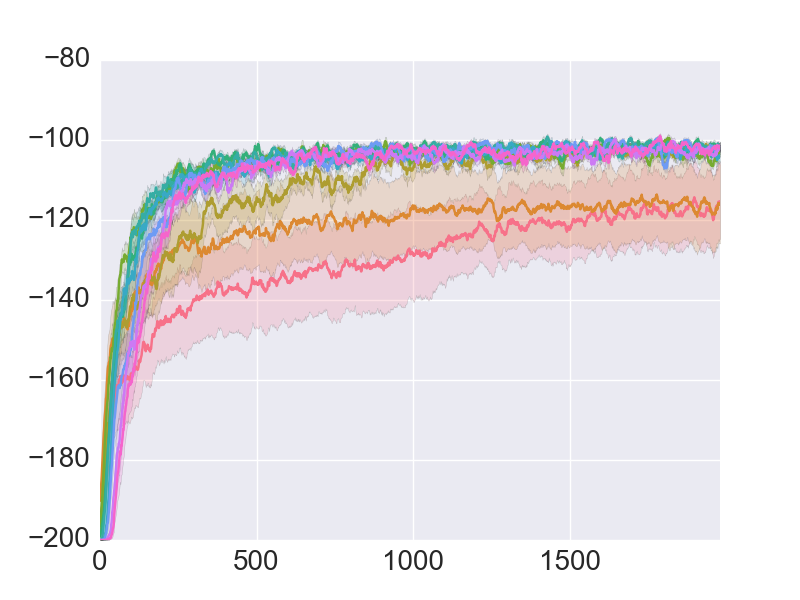
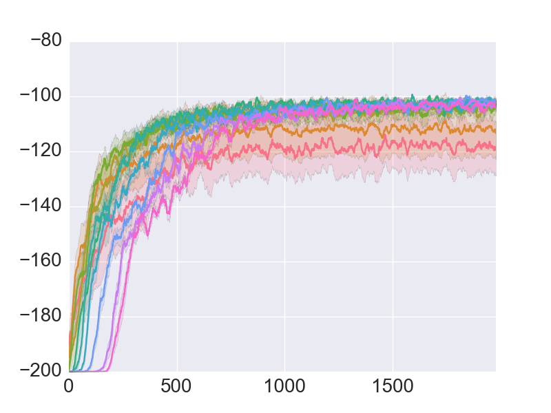
Figure 1 shows the results on this problem for a range of values without step-size tuning. values were chosen as powers of which range from excessively low to too high to allow learning. Figure 2 shows the results of Normalized Scalar Metatrace for a range of values. For a fairly broad range of values, learning curves of different values are much more similar compared to without tuning.


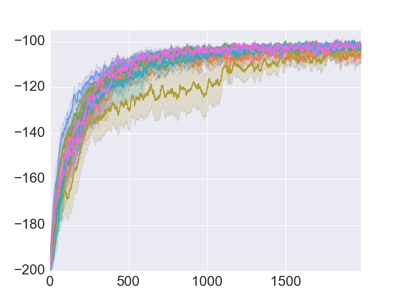
Figure 3 shows the performance of Unnormalized Scalar Metatrace over a range of and initial values. As in Figure 2 for Normalized Scalar Metatrace, for a fairly broad range of values, learning curves over different initial values are much more similar compared to without tuning. Two qualitative differences of the normalized algorithm over the unnormalized version are: (1) the useful values are much larger, which for reasons outlined in [15] likely reflects less problem dependence, and (2) the highest initial alpha value tested, , which does not improve at all without tuning, becomes generally more stable. In both the normalized and unnormalized case, higher values than those shown cause increasing instability.


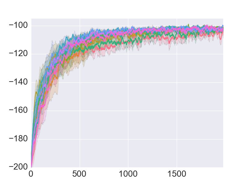
We performed this same experiment for SID and NOSID [2], modified for AC rather than SARSA. These results are presented in Figures 4 and 5. We found that the unnormalized variants of the two algorithms behaved very similarly on this problem, while the normalized variants showed differences. This is likely due to differences in the normalization procedures. Our normalization procedure is based on that found in [8]. The one used by NOSID is based on that found in [14]. The normalization of NOSID seems to make the method more robust to initial values that are too high, as well as maintaining performance across a wider range of values. On the other hand, it does not shift the useful range of values up as much66 6 NOSID becomes unstable around , again potentially indicating more variation in optimal value across problems. Additionally, the normalization procedure of NOSID makes use of a hard maximum rather than a running maximum in normalizing the update, which is not well suited for non-stationary state representations where the appropriate normalization may significantly change over time. While this problem was insufficient to demonstrate a difference between SID and Metatrace, we conjecture that in less sparse settings where each weight is updated more frequently, the importance of incorporating the correct time index would be more apparent. Our ALE experiments certainly fit this description, however we do not directly compare with the update rule of SID in the ALE domain. For now, we note that [2] focuses on the scalar case and does not extend to vector valued . Comparing these approaches more thoroughly, both theoretically and empirically, is left for future work.




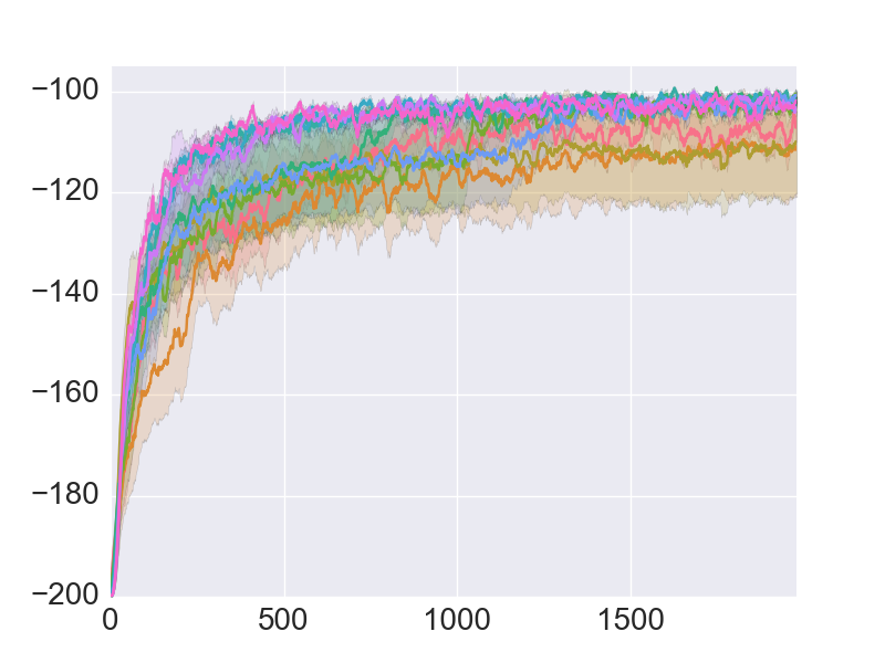
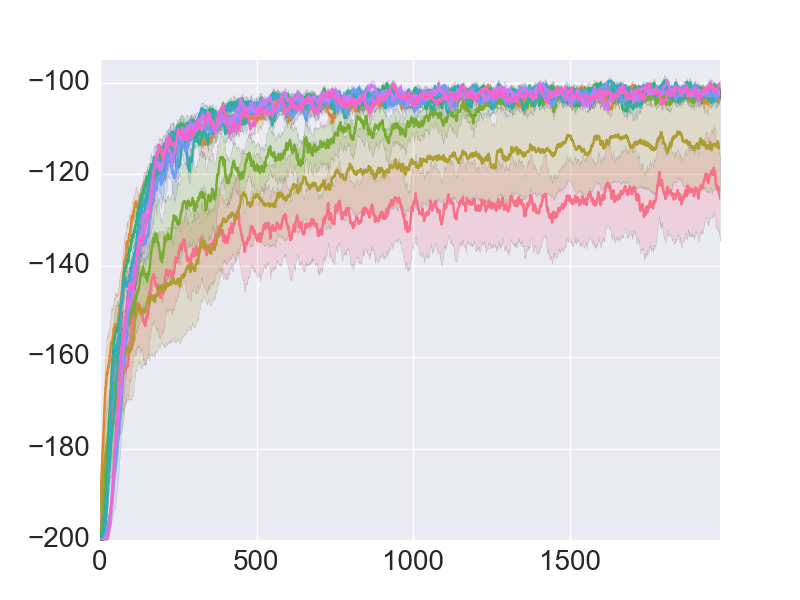
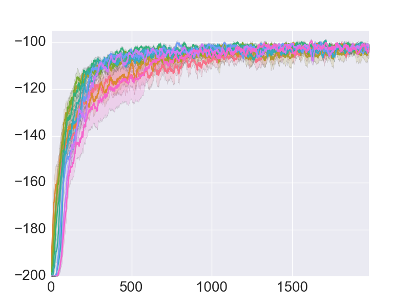
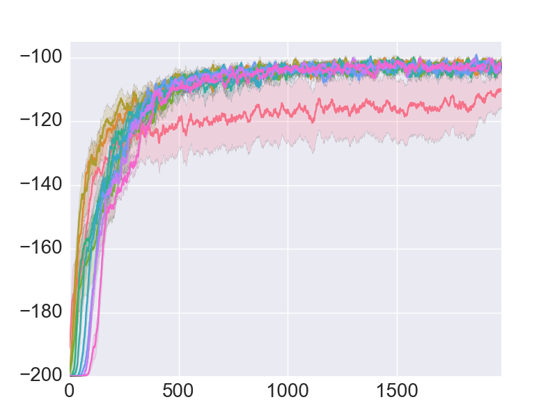
Vector Metatrace is much less effective on this problem (results are omitted). This can be understood as follows: the tile-coding representation is sparse, thus at any given time-step very few features are active. We get very few training examples for each value when vector step-sizes are used. Using a scalar step-size generalizes over all weights to learn the best overall step-size and is far more useful. On the other hand, one would expect vector step-size tuning to be more useful with dense representations or when there is good reason to believe different features require different learning rates. An example of the later is when certain features are non-stationary or very noisy, as we will demonstrate next.
5.2 Drifting Mountain Car
Here we extend the mountain car domain, adding noise and non-stationarity to the state representation. This is intended to provide a proxy for the issues inherent in representation learning (e.g., using a NN function approximator), where the features are constantly changing and some are more useful than others. Motivated by the noisy, non-stationary experiment from [15], we create a version of mountain car that has similar properties. We use the same tiling features as in the mountain car case but at each time-step, each feature has a chance to randomly flip from indicating activation with to and vice-versa. We use a uniform flipping probability per time step across all features that we refer to as the drift rate. Additionally we add noisy features which are 1 or 0 with probability for every time-step. In expectation, will be active on a given time-step. With tilings, informative features will also be active, thus in expectation half of the active features will be informative.
Due to non-stationarity, an arbitrarily small is not asymptotically optimal, being unable to track the changing features. Due to noise, a scalar will be suboptimal. Nonzero values for noisy features lead to weight updates when that feature is active in a particular state; this random fluctuation adds noise to the learning process. This can be avoided by annealing associated s to zero.
Figure 6 shows the best value tested for several drift rate values for scalar, vector, and mixed Metatrace methods along with a baseline with no tuning. All methods learn quickly initially before many features have flipped from their initial value. Once many features have flipped we see the impact of the various tuning methods. Mixed Metatrace performs the best in the long run so there is indeed some benefit to individually tuning s on this problem. Scalar Metatrace is able to accelerate early learning but at the higher drift values eventually drops off as it is unable to isolate the informative features from the noise. Vector Metatrace tends to under-perform scalar near the beginning but eventually surpasses it as it is eventually able to isolate the informative features from the noise.


Figure 7 a, c and e show all values tested for each method for one drift rate value to indicate the sensitivity of each method to . The general pattern is similar for a broad range of values. Figure 7 b, d and f show how the average values for different weights evolve over time for the various methods. Both vector and mixed metatrace show much stronger separation between the noisy and informative features for the value function than for the policy. One possible explanation for this is that small errors in the value function have far more impact on optimizing the objective in mountain car than small imperfections in the policy. Learning a good policy requires a fine-grain ability to distinguish the value of similar states, as individual actions will have a relatively minor impact on the car. On the other hand, errors in the value function in one state have a large negative impact on both the value learning of other states and the ability to learn a good policy. We expect this outcome would vary across problems.
5.3 Arcade Learning Environment
Here we describe our experiments with the 5 original training set games of the ALE (asterix, beam rider, freeway, seaquest, space invaders). We use the nondeterministic ALE version with repeat_action_probability = 0.25, as endorsed by [9]. We use a convolutional architecture similar to that used in the original DQN paper [12]. Input was 84x84x4, downsampled, gray-scale versions of the last 4 observed frames, normalized such that each input value is between 0 and 1. We use frameskipping such that only every frame is observed. We use 2 convolutional layers with 16 8x8 stride 4, and 32 4x4 stride 2 filters, followed by a dense layer of 256 units. Following [4], activations were dSiLU in the fully connected layer and SiLU in the convolutional layers. Output consists of a linear state value function and softmax policy. We fix and and use entropy regularization with . For Metatrace we also fix , a value that (based on our mountain car experiments) seems to be reasonable. We run all experiments up to 12.5 million observed frames77 7 Equivalent to 50 million emulator frames when frame skipping is accounted for..
We first performed a broad sweep of values with only one repeat each for each of the 3 tuning methods, and an untuned baseline on seaquest to get a sense of how the different methods perform in this domain. While it is difficult to draw conclusions from single runs, the general trend we observed is that the scalar tuning method helped more initial values break out of the first performance plateau and made performance of different initial values closer across the board. Scalar tuning however did not seem to improving learning of the strongest initial s. Vector and mixed tuning, on the other hand, seemed to improve performance of near optimal s as well as reducing the discrepancy between them, but did not seem to help with enabling weaker initial values to break out of the first performance plateau. Note also, likely owing in part to the normalization, with each tuning method the highest tested is able to improve to some degree, while it essentially does not improve at all without tuning.


After this initial sweep we performed more thorough experiments on the 5 original training set games using mixed Metatrace with the 3 best values found in our initial sweep. Additionally, we test a baseline with no tuning with the same values. We ran 5 random seeds with each setting. Figure 10 shows the results of these experiments.
Metatrace significantly decreases the sensitivity to the initial choice of . In many cases, metatrace also improved final performance while accelerating learning. In space invaders, all 3 values tested outperformed the best with no tuning, and in seaquest 2 of the 3 did. In asterix, the final performance of all initial s with Metatrace was similar to the best untuned alpha value but with faster initial learning. In beam rider, however, we see that using no tuning results in faster learning, especially for a well tuned initial . We hypothesize that this result can be explained by the high sensitivity and slow initial learning speed in beam rider. There is little signal for the tuning to learn from early on, so the values just drift due to noise and the long-term impact is never seen. In future work it would be interesting to look at what can be done to make Metatrace robust to this issue. In freeway, no progress occurred either with or without tuning.


6 Conclusion
We introduce Metatrace, a novel set of algorithms based on meta-gradient descent, which performs step-size tuning for AC. We demonstrate that Scalar Metatrace improves robustness to initial step-size choice in a standard RL domain, while Mixed Metatrace facilitates learning in an RL problem with non-stationary state representation. The latter result extends results of [15] and [8] from the SL case. Reasoning that such non-stationarity in the state representation is an inherent feature of NN function approximation, we also test the method for training a neural network online for several games in the ALE. Here we find that in three of the four games where the baseline was able to learn, Metatrace allows a range of initial step-sizes to learn faster and achieve similar or better performance compared to the best fixed choice of .
In future work we would like to investigate what can be done to make Metatrace robust to the negative example we observed in the ALE. One thing that may help here is a more thorough analysis of the nonlinear case to see what can be done to better account for the higher order effects of the step-size updates on the weights and eligibility traces, without compromising the computational efficiency necessary to run the algorithm on-line. We are also interested in applying a similar meta-gradient descent procedure to other RL hyperparameters, for example the bootstrapping parameter , or the entropy regularization parameter . More broadly we would like to be able to abstract the ideas behind online meta-gradient descent to the point where one could apply it automatically to the hyperparameters of an arbitrary online RL algorithm.
Acknowledgements
The authors would like to acknowledge Pablo Hernandez-Leal, Alex Kearney and Tian Tian for useful conversation and feedback.
References
- [1] Brockman, G., et al.: Open AI Gym. arXiv preprint arXiv:1606.01540 (2016).
- [2] Dabney, W.C.: Adaptive step-sizes for reinforcement learning. Doctoral Dissertations. 173. https://scholarworks.umass.edu/dissertations_2/173 (2014).
- [3] Degris, T., Pilarski, M.P., and Sutton, R.S.: Model-free reinforcement learning with continuous action in practice. American Control Conference (ACC), IEEE, 2012.
- [4] Elfwing, S., Uchibe, E., and Doya, K.: Sigmoid-weighted linear units for neural network function approximation in reinforcement learning. Neural Networks (2018).
- [5] Kearney, A., Veeriah, V., Travnik, J., Sutton, R., Pilarski, P.M.: Every step you take: Vectorized Adaptive Step-sizes for Temporal-Difference Learning. 3rd Multidisciplinary Conference on Reinforcement Learning and Decision Making. 2017. (Poster and abstract.)
- [6] Kearney, A., Veeriah, V., Travnik, J., Sutton, R., Pilarski, P.M.: TIDBD: Adapting Temporal-difference Step-sizes Through Stochastic Meta-descent. arXiv preprint arXiv:1804.03334 (2018). (v1 from May 19, 2017).
- [7] Kingma, D.P., Ba, J.: Adam: A method for stochastic optimization. arXiv preprint arXiv:1412.6980 (2014).
- [8] Mahmood, A.R., et al.: Tuning-free step-size adaptation. Acoustics, Speech and Signal Processing (ICASSP), IEEE, 2012.
- [9] Machado, M.C., et al.: Revisiting the Arcade Learning Environment: Evaluation Protocols and Open Problems for General Agents. JAIR 61, 523-562 (2018)
- [10] Mnih, V., et al.: Asynchronous methods for deep reinforcement learning. International Conference on Machine Learning. 2016.
- [11] Mnih, V., et al.: Human-level control through deep reinforcement learning. Nature 518, 529-533. (2015)
- [12] Mnih, V., et al.: Playing atari with deep reinforcement learning. arXiv preprint arXiv:1312.5602 (2013).
- [13] Schulman, J., et al.: High-dimensional continuous control using generalized advantage estimation. arXiv preprint arXiv:1506.02438 (2015).
- [14] Ross, S., Mineiro, P. and Langford, J.: Normalized online learning. arXiv preprint arXiv:1305.6646 (2013).
- [15] Sutton, R.S.: Adapting bias by gradient descent: An incremental version of delta-bar-delta. AAAI. 1992.
- [16] Sutton, R.S., et al.: Policy gradient methods for reinforcement learning with function approximation. Advances in neural information processing systems. 2000.
- [17] Tieleman, T., Hinton, G.: Lecture 6.5-rmsprop: Divide the gradient by a running average of its recent magnitude. COURSERA: Neural networks for machine learning 4.2 (2012): 26-31.
- [18] Van Hasselt, H., Guez, A., and Silver, D.: Deep Reinforcement Learning with Double Q-Learning. AAAI. Vol. 16. 2016.
- [19] Veeriah, V., Zhang, S., Sutton. R.S.: Crossprop: Learning Representations by Stochastic Meta-Gradient Descent in Neural Networks. ECML. 2017